Stochastic Poisson Surface ReconstructionJournal: TOGVolume: 41622712DOI: 10.1145/3550454.3555441

Abstract.
We introduce a statistical extension of the classic Poisson Surface Reconstruction algorithm for recovering shapes from 3D point clouds. Instead of outputting an implicit function, we represent the reconstructed shape as a modified Gaussian Process, which allows us to conduct statistical queries (e.g., the likelihood of a point in space being on the surface or inside a solid). We show that this perspective: improves PSR’s integration into the online scanning process, broadens its application realm, and opens the door to other lines of research such as applying task-specific priors.
1. Introduction
Surface reconstruction refers to the process of converting a point cloud (the most common real-world raw 3D capture format) into another shape representation, such as a mesh or an implicit function, for use in downstream applications. This is an underdetermined process filled with uncertainty, not just due to a point cloud’s discrete nature and lack of topological information but also because of real-world challenges like scan occlusions or measurement error.
The de facto standard geometry processing algorithm for this task is Poisson Surface Reconstruction (PSR) [Kazhdan et al. 2006], which solves a partial differential equation to reconstruct a function whose zero levelset defines the desired surface. Due to its speed, quality and simplicity, PSR remains relevant and has seen uses in fields as varied as digital heritage preservation [Andrade et al. 2012], topography [Gupta and Shukla 2017], medicine [Palomar et al. 2016] and autonomous driving [Vizzo et al. 2021].

Unfortunately, PSR lacks the statistical formalism to quantify the uncertainties of the surface reconstruction process. The magnitudes of outside of the zero levelset are arbitrary (see Fig. 2) and alone cannot provide an answer to statistical questions crucial to the reconstruction process like “how confident can one be of the values of ?” or “where should one aim the scanner next to optimize information gain?” Similarly, it cannot respond to queries like “what is the probability of a point being contained in the shape?”, critical for collision detection or ray casting applications.
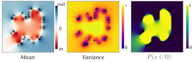
In this paper, we introduce Stochastic Poisson Surface Reconstruction (SPSR), a statistical derivation of PSR as conditional probability distributions in a Gaussian Process (GP). Instead of just an implicit function value, we endow every point in space with a Gaussian distribution of possible values. We propose an algorithm to compute the mean and variance that fully determine this distribution (see Fig. 1), allowing us to answer any statistical queries.
This extension vastly broadens the use cases of Poisson Surface Reconstruction, as we highlight with prototypical examples of surface point cloud repair, ray casting, next-view planning and collision detection. Furthermore, we show that by understanding PSR from this new perspective, we can borrow from the Gaussian Process literature to modify it by incorporating task-specific priors, opening several promising lines of future research.
2. Related Work

A complete survey of vast research areas like uncertainty quantification or surface reconstruction is beyond the scope of this work. Instead, we focus this section on setting our Stochastic PSR in its context of bridging the gap between PSR and Gaussian Processes.
2.1. Surface Reconstruction from Point Clouds
Point clouds are a common raw format for 3D geometry acquired form the real world. However, most applications in fields like rendering, simulation and geometry processing require more structured representations like triangle meshes. Thus, reconstructing surfaces from point clouds is a well-studied, fundamental problem in Computer Graphics (see [Berger et al. 2017] for an exhaustive survey). While some methods convert point clouds directly to meshes (e.g., by dictionary learning [Xiong et al. 2014]) or simple primitives (e.g., [Monszpart et al. 2015; Nan et al. 2010]), we focus on those that extract the shape as the zero levelset of a reconstructed function .
Within these, a common separation is made between local and global algorithms. Local algorithms prioritize performance in speed and memory; for example, by fitting linear [Hoppe et al. 1992], polynomial [Alexa et al. 2001] or higher-order [Fuhrmann and Goesele 2014] functions to restricted point subsets. By their nature, these are more susceptible to oscillations far from the sample points. To cope, global algorithms (e.g., [Jacobson et al. 2013]) allow to be influenced by every point in the cloud (hierarchical fast summation structures can help reduce computation [Barill et al. 2018]).
Poisson Surface Reconstruction (PSR) [Kazhdan et al. 2006] captures the best features of the global (robustness) and local (performance) methods by computing in two steps. First, a vector field is interpolated from the point cloud using only local information. Then, is obtained from via a global sparse PDE solve, which is discretized as a linear system and can be solved very efficiently using an adaptative grid structure. PSR has been improved since its publication; for example, Kazhdan and Hoppe 2013 combine both steps to improve noise robustness, Kazhdan et al. 2020 include envelope constraints and Peng et al. 2021 formulate the Poisson solve in a differentiable way. Nonetheless, the original 2006 publication is still one of the few showing robustness in every metric considered by Berger et al. 2017 more than a decade later.
Our Stochastic PSR inherits all the benefits of the original PSR, supplying it with a complete statistical formalism that extends it and its application realm (see Fig. 3). Our contributions are orthogonal to the specific grid structure used (see [Kazhdan and Hoppe 2019]).
Our algorithm can output the probability of any point in space being inside the sampled domain (see Fig. 1). While this resembles the shape representations proposed by occupancy networks [Mescheder et al. 2019] and neural radiance fields [Mildenhall et al. 2020], we note that our algorithm produces this quantity as a direct byproduct of a fully determined statistical distribution which can answer many other statistical queries, like boundary probabilities (see Fig. 5) or regional probabilities (see Fig. 12).


2.2. Gaussian Processes
A Gaussian Process (GP) is an infinite collection of joint normal distributions [Doob 1944; Dudley 2018], usually parametrized by a continuous parameter like time or space [Kac and Siegert 1947]. Recently, Gaussian processes have been used as a tool in unsupervised learning (see [Williams and Rasmussen 2006] for an introduction, [Engel et al. 2005; Raissi et al. 2017] for examples), even suggested initially as an alternative to neural networks by MacKay 1997.
Closer to our application are Gaussian Process Implicit Surfaces (GPIS) [Williams and Fitzgibbon 2006]. These algorithms exchange the function that implicitly defines a surface for a Gaussian distribution , and compute and by studying the posterior GP distribution given observed points. One can recover a surface by extracting the zero levelset of ; however, the information contained in also finds use in tasks like robotic grasping [Dragiev et al. 2011], next view planning [Hollinger et al. 2012] and segmentation [Shin et al. 2017; Ramon Soria et al. 2017].
GPIS present the same global/local dilemma as other surface reconstruction algorithms. If the interpolation is done using all the point cloud information (this is encoded in the support of the GP covariance function), the method suffers in performance; if not, in robustness. By using the insights of Poisson Surface Reconstruction, our Stochastic PSR instead uses a local Gaussian Process to build the distribution of the gradient field , and then recover the full distribution of with a global PDE solve. While using a GP to interpolate vector-valued data is unorthodox, we note it has been done before; e.g., for fluid velocity information [Lee et al. 2019].
Gaussian processes are a more traditional approach to quantifying the uncertainty of a regression model, a field which has seen significant growth since recent advances in deep learning (see [Abdar et al. 2021] for a survey). Often, the posterior distribution of a given neural network is approximated by another Bayesian network whose parameters minimize a chosen distribution loss. (see e.g., [Xue et al. 2019]). Alternatively, the posterior may be learned directly from the observed data (see e.g., [Shen et al. 2021]).

2.3. Stochastic Geometry Processing
Our algorithm stands among many similar works that add statistical formalism to standard geometry processing techniques, like point cloud registration. Specifically, a lot of work has been dedicated to computing the covariances in the pairwise iterative closest point [Landry et al. 2019; Bosse and Zlot 2008] and, most recently, for general multi-scan registration [Cao et al. 2018; Huang et al. 2020].
Closer to our application, Curless and Levoy 1996 compute truncated signed distance fields for each sensor position and use a model for their individual uncertainty to weigh their contributions to the final implicit reconstruction. Pöthkow et al. 2011 model grid samples of an implicit function as normal distributions and calculate the individual probabilities of each voxel marching cubes configuration to quantify the contouring uncertainty. Sharf et al. 2007 similarly measure topological reconstruction uncertainty to identify where user-provided disambiguation is most needed.
Pauly et al. 2004 work is the most similar to ours. It takes a point cloud as input and uses a surface smoothness prior to compute the likelihood of any point in space lying on it (see Fig. 5, left). Instead, our proposed algorithm assumes samples to lay on the boundary of a solid, and impose solid smoothness prior (examined further in Section 5). Further, while our algorithm can also output a surface likelihood quantity (see Fig. 5, center), it is only part of a full statistical distribution of the solid (see Fig. 5, right).
3. Background
By posing PSR as a Gaussian Process, our work combines these two concepts. We begin by reviewing them individually.
3.1. Gaussian Processes
Intuitively, a Gaussian Process is an extension of the multivariate normal distribution to an infinite number of dimensions. Formally, let be a collection of random variables parametrized by some continuous parameter . is said to be a Gaussian Process if any finite subset of follows a multivariate Gaussian distribution. Equivalently, is a Gaussian Process if for any two ,
| (1) |
for some mean and covariance functions , . These two functions uniquely determine the Gaussian Process .
Gaussian Processes are a particularly useful tool for supervised learning tasks (see Fig. 4). Assume training observations , where each is an observation of the distribution , and consider an unobserved (test) point . By definition of GP, the joint distribution of is
| (2) |
which we write as
| (3) |
where it is relevant to note that depends only on the training data and depends on both training and test sets. By Bayes’ theorem, this means the distribution of conditioned on the observations is
| (4) |
One usually assumes (otherwise, the Gaussian process is considered), and writes
| (5) |
In the case of noisy observations, a term (where is the noise variance) is added to .

3.2. Poisson Surface Reconstruction
Any input oriented point cloud of the surface of a solid shape can be written as a set of observations , each of them storing a position and a (normalized) orientation . Poisson Surface Reconstruction [Kazhdan et al. 2006] aims to build a function which takes positive values inside and negative values outside of it, thus making the zero levelset the reconstructed surface .
PSR begins by building a grid . Then, they define the following vector field for any by using the grid structure to interpolate the orientation observations:
| (6) |
where are the eight closest grid nodes to , is the trilinear interpolation weight for at , is a measure of volumetric sampling density and is a compactly-supported approximation of a Gaussian kernel centered at the -th node.
The fundamental observation of PSR is that once has been constructed, the desired implicit function satisfies
| (7) |
Eq. (7) is underdetermined, as wildly different functions can have the same Laplacian. This ambiguity is resolved in part during discretization. Kazhdan et al. 2006 suggest building as an adaptive grid of a bounding box of the point cloud. Then, they use the finite element method to build discrete Laplacian and divergence operators and and solve
| (8) |
This discretization imposes zero Neumann boundary conditions on the boundary of . Even so, Eq. (8) only determines up to translation. To account for this, one valid is computed and then shifted so its values near the observation points are zero on average. The solution contains the implicit function evaluated at each grid node, and its zero levelset can be extracted using contouring algorithms like Marching Cubes [Lorensen and Cline 1987] or Dual Contouring [Ju et al. 2002].
4. Stochastic Poisson Surface Reconstruction
We introduce our Stochastic PSR, which extends the traditional PSR from Kazhdan et al. 2006 with the statistical formalism of a Gaussian Process. We begin by defining the PSR semicovariance as
| (9) |
where is a scalar parameter. Then, the vector field interpolation in Eq. (6) can be written as
| (10) |
By term identification, it may be tempting to interpret this interpolation directly as the posterior mean of a Gaussian Process (see Eq. (5)), with normals as the observed values , as the entries of and division by playing the role of multiplication by . However, a valid Gaussian distribution must have a symmetric covariance, and in general (hence the semi in “PSR semicovariance”). To circumvent this, we define the Stochastic PSR covariance to be its symmetrized version
| (11) |
which analagously defines a Stochastic PSR vector field
| (12) |
This variance symmetrization will be our only deviation from the traditional Poisson Surface Reconstruction by Kazhdan et al. 2006 (see Fig. 8). Strictly speaking, all the observations that follow in this paper can only be said to apply to ; however, note that and are visually indistinguishable (see Fig. 7) and their difference vanishes under refinement (see proof in Appendix A).
Our critical observation is that the interpolation in Eq. (12) can be interpreted as the mean of a supervised learning task under the assumptions of a Gaussian Process with and covariance . Indeed, one needs only to exchange for the vector-valued and the observations for in Eq. (5) to obtain the conditional probability distribution
| (13) |
where
| (14) | |||
| (15) |
The main computational cost in computing the mean and variance of the conditional distribution is the inversion of , a matrix whose size scales with the number of points in the cloud. One could avoid this by assuming that the samples are independent, which would result in approximating by . However, completely discarding the sample interdependency could have adverse effects: in practice, it would make densely sampled regions have an outsized effect over more sparsely sampled ones (see Fig. 9, center right).
We introduce a better approximation: we assume each sample is independent, but with variance proportional to sampling density. Intuitively, this means we account for the interdependence by trusting each individual sample in a densely sampled region less than in a sparsely sampled one (see Fig. 9, right). We justify this choice mathematically in the general GP context in Appendix B.
We are not aware of any previous work that proposes this approximation, which addresses one of the main performance limitations of general Gaussian Processes. Numerically, this resembles the mass matrix lumping step often carried out in the Finite Element literature (see e.g., [Zienkiewicz et al. 2005] Chap. 16.2.4.), so we call it the (diagonal) lumped covariance matrix
| (16) |
where is the local sampling density at each sample point, which we compute as described by Kazhdan et al. 2006. As is usual with Gaussian processes, we sum if the sampled point cloud is assumed to contain noise with variance in the normal vector.
Then, the conditional distribution becomes
| (17) |
Importantly, note that the mean of this distribution is exactly the Stochastic PSR vector field we introduced in Eq. (12), i.e.,
| (18) |
In other words, this critical reinterpretation of PSR has allowed us to extend the interpolated PSR vector field into a complete statistical distribution whose mean is nearly identical to (see Fig. 7, which we can now understand as comparing the traditional PSR vector field to the mean of our lumped Gaussian Process).
Ideally, however, we would want a similar statistical formalism not for but for the implicit function , which would allow us to formulate statistical queries meaningful to the reconstruction task, e.g., .

Fortunately, transfering our statistical understanding of to is just a matter of Gaussian arithmetic. First, note that a reasoning identical to the one above leads to the joint conditional probability of at all grid nodes being
| (19) |
where
| (20) |
and
| (21) |
For simplicity, denote , and let be the concatenated vector of values as in the previous section. Then, Eq. (19) becomes
| (22) |
By linearity and bilinearity of the mean and covariance, respectively, we know
| (23) |
and thus, since the vector of evaluations of satisfies ,
| (24) |
Similarly to the traditional PSR, we shift the mean values to be zero near the sample points and shift the variance values to have a minimum diagonal entry of zero. We write the above distribution as
| (25) |
This statement is our principal contribution, as it extends the traditional PSR implicit function into a full statistical distribution whose mean is almost identical to . Of all the information contained in , a particularly useful quantity is its diagonal , which contains the variances of each entry of (see Fig. 3).
4.1. Statistical queries
Eq. (25) contains all the information we need to respond to statistical queries fundamental to the reconstruction process; e.g., the probability of a given point being inside the shape (see Fig. 10)
| (26) |
or the probability density of being on the surface (see Fig. 13)
| (27) |
where and are the cummulative distribution and probability density functions, respectively, of a Gaussian distribution with mean and variance . Similar Gaussian arithmetic lets us compute other quantities like confidence intervals (see Fig. 14).

All these queries would be impossible to answer from PSR’s alone. We show this in the didactic example in Fig. 6, where vectors pointing upward are sampled from a normal distribution centered at the middle horizontal line. As more samples get added, converges to a smooth transition between positive and negative values; however, our variances are progressively decreasing, making converge in certainty as expected.
We formalize this observation further by defining an integrated statistical quantity, the total uncertainty , which we define as
| (28) |
where is a bounding box around the point cloud. can be intuitively interpreted as a global measure of reconstruction quality which converges to zero when the surface has been reconstructed with absolute certainty (see Fig. 15). We pose that this quantity can be used as a stopping criteria to guide the scanning process (see Fig. 17). We know of no analogous quantity that can be formally defined from the traditional PSR understanding alone.


The off-diagonal entries of quantify the correlation between the values of at different points in . This allows for joint probability queries; for example, computing the likelihood of a whole region in space intersecting (see Fig. 12), a quantity of immediate relevance to collision detection applications.
To compute it, we can randomly sample . If is the linear interpolation matrix from to , then distribution arithmetic says
| (29) |
The collision probability, i.e., the probablity that any is contained in the shape, is opposite to the joint probability that all are outside the shape, . This quantity is also the same as , known as the multivariate Gaussian cummulative distribution of , which can be estimated with numerical integration (see Figs. 12 and 20).
4.2. Space reduction with eigenspace analysis
All this additional information comes at a computational cost. Specifically, the main performance bottleneck is the computation of the covariance matrix
| (30) |
a matrix equation that amounts to solving linear systems. Even making use of efficient prefactorizations of , this step is impracticable for large 3D grids with sizes in the millions of cells.
To circunvent this, we will work in the reduced space of Laplacian eigenvectors. For a cuboid with lengths and zero Neumann boundary conditions, these are known [Gottlieb 1985] to respond to the analytic function
| (31) |
with associated eigenvalues
| (32) |
Specifically, we will evalute these analytical expressions into , the matrix of the lowest-magnitude eigenvectors of , and , the diagonal eigenvalue matrix. Then, we approximate by projecting to the eigenspace, solving the matrix equation in this reduced space, and reprojecting; i.e.,
| (33) |
In all our examples, we fix .
Due to the dimensionality of the above matrices, the mostly computationally expensive step in Eq. (33) is the product , where results from multiplying all middle matrices in Eq. (33). We avoid this step by noting that it is rare that one is interested in all entries of . As seen in Section 4.1, most statistical queries require only the diagonal , which we can compute directly and efficiently as , where denotes row-wise dot product. In the case of joint probability queries that require off-diagonal knowledge of , we first construct the selection matrices that extract the covariance rows and columns relevant to the specific application, and directly compute , where . Thus, we eventually avoid ever computing (or storing) the full .
Dimension reduction has been used for implicit reconstruction before; e.g., the Fourier coefficients computed by Kazhdan 2005. We limit our approximation to the covariance computation only.
4.3. Adaptive discretization


The statistical formalism we contribute is agnostic to where the values of and are stored and to the discretization scheme used to solve the Poisson equation. Kazhdan et al. 2006 suggest building an adaptive grid which is finer near the sampled point cloud. This choice is justified through their sole goal of accurately recovering the zero levelset of .
Our Stochastic PSR extends the traditional PSR by providing volumetric statistical information, which is also relevant and non-trivial in regions away from the zero levelset of our mean function or the point cloud (see, e.g., the probability in Fig. 10). Further, computing statistical queries accurately away from the mean-zero levelset can be critical for applications that our formalism newly allows like collision detection or ray casting (see Fig. 24). Thus, the choice of an adaptive grid structure is less obvious for our algorithm. Nonetheless, we show in Fig. 16 our algorithm working as expected on a graded quadtree grid structure, following the finite difference discretization proposed by Bickel et al. 2006. While orthogonal to our contribution, we believe exploring different adaptive discretization strategies (e.g., narrowing in on regions of higher uncertainty) to be a promising avenue for future work.
5. Beyond Poisson Surface Reconstruction
A significant benefit of our interpretation of Poisson Surface Reconstruction as a Gaussian Process is that we may borrow from the vast literature on the latter to study variations of the traditional PSR. A prototypical example of this is incorporating task-specific priors.
In Section 3.1, we mentioned that most Gaussian Process consider and are thus fully determined by the covariance (this is often known as kriging in the GP literature). Indeed, it was by assuming that we recovered the PSR vector field interpolation as the mean of the GP posterior distribution. In fact, the choice of is a prior imposed on the joint distribution before any data is observed. Thus, PSR can be understood to have a zero-gradient prior.
Incidentally, this observation also provides an answer to an often asked question about PSR; namely, why PSR, which is posed as recovering a function which is zero on the surface and satisfies certain norm-one gradients, produces an output so different from a Signed Distance Field (SDF). From this novel Gaussian Process perspective, we can understand that PSR is, via its prior, encouraging zero-norm gradients away from the sample positions, while an SDF requires Eikonal norm one gradients almost everywhere.
Primitive geometric priors.
Martens et al. 2016 suggest using simple geometric primitives as priors in the context of GP implicit surfaces. Since the authors are directly learning the surface’s implicit representation, their suggested priors are scalar, SDF-like functions. In our case, where learning is carried out in the gradient space and then transfered to an implicit function via a PDE solve, we can use gradient vector-valued priors.
In Fig. 19, we exemplify the effect of a simple spherical prior
| (34) |
which we pose can be a useful tool for favouring closed reconstructions over open ones. is a parameter tuning the strength of the prior and is the center of the sphere, which we set to be the average of all point cloud positions. In Fig. 18, we show less didactical uses of this same prior, along with a similar ellipsoidal one.
6. Implementation details
We implemented our algorithm in Python, using libigl [Jacobson et al. 2018] for common geometry processing subroutines. We rendered all our figures in Blender, using BlenderToolbox [Liu 2022]. All our results were produced on our machine with Intel Xeon CPU E5-2637 v3 3.50Hz (16 cores) with 64GB of RAM.
For parameter standardization, we normalized all our examples to fit a length-one cube as a preprocessing step. Unless specified otherwise, we use a uniform grid ( in the two-dimensional examples) such that and become the usual finite difference Laplacian and divergence matrices. We fix , and . We use the same function as Kazhdan et al. 2006, obtained by convolving a box filter with itself three times.
For memory efficiency, we use SciPy’s biconjugate gradient method to solve for the distribution mean , which accounts for approximately of our runtime (around seconds in all 3D examples). Our main computational bottleneck is Eq. (33) (specifically, the projection of into the reduced space), covering of our runtime (around two minutes in all 3D examples).


7. Experiments
7.1. Deviation from Kazhdan et al. 2006
Our sole deviation from traditional Poisson Surface Reconstruction as introduced by Kazhdan et al. 2006 is the symmetrization of the covariance in Eq. (37). Theoretically, it is clear that both and converge to the same symmetric in the limit of grid refinement. However, we also justify the step by showing that the difference between these two is small even at a very coarse resolution in Fig. 8. In PSR, is used to reconstruct a vector field . In Fig. 7, we show that the interpolated vector field obtained with the symmetrized covariance is visually identical. In Fig. 3, we show that this applies also to the implicit function obtained through the Poisson solve.
7.2. Statistical quantities
Our Stochastic PSR exchanges the functional PSR output for a fully defined statistical distribution. To explore just how much more information is contained in this distribution, we show different statistical quantities meaningful to the shape reconstruction process.
In Fig. 10, we use our computed mean and variance to evaluate each point’s cummulative distribution functions at zero, which returns the probability of any point in space being contained in . Similarly, evaluating the probabilistic density function at zero returns a measure of surface probability, as we show in Fig. 13. We use slice planes to visualize these functions for a 3D reconstruction problem in Fig. 1 and Fig. 11. In Fig. 14, we show our statistical formalism applied to the computation of confidence intervals, which serve as an intuitive tool for visualizing variances.
8. Applications
Our main contribution is a novel theoretical understanding of Poisson Surface Reconstruction that expands it beyond its traditional application realm. We explore this with prototypical results.
8.1. Collision detection
Statistical information is critical for robots or autonomous vehicles, which may capture their surroundings as point clouds with partial occlusions. When a car is deciding whether to swerve, it does not want to know only if the maneuvre is secure for the most likely scenario of its surroundings (the traditional PSR output or the SPSR mean); rather, it must account for uncertainty and conclude whether the maneuvre is safe in the vast majority of possible scenarios.
We exemplify this in Fig. 20, where we simulate a 3D scan of a street and use joint probability queries to compute the collision chance of an automated vehicle along a given trajectory. We compare this chance against a baseline (in grey), which only checks for intersections between the car mesh and the traditional PSR zero isolevel extracted with Marching Cubes [Lorensen and Cline 1987]. We include synthetic Gaussian noise both on the input point positions and normal vectors. In Fig. 22, we show how one can threshold our computed probabilities to obtain isosurfaces for use in collision detection applications.

8.2. Volume rendering
The arbitrary units in the traditional PSR output mean that it cannot be interpreted as a volume rendering occupancy. Fortunately, our Stochastic Poisson Surface Reconstruction allows us to compute , values between 0 and 1 which can be interpreted as occupancies (this reinterpretation is common in the Neural Radiance Field literature, e.g., [Mildenhall et al. 2020]). In Fig. 24, we use standard volume rendering techniques (see [Pharr et al. 2016], Chap. 11) to sample the free path of a ray aimed at a partial reconstruction of a Space Wizard vehicle from two different directions. As expected, rays intersecting regions with higher uncertainty produce a wider spread of paths, as evidenced by the orange and blue histograms.
8.3. Reconstruction
Scanning integration
Surface reconstruction is the flagship application of PSR. Despite this, PSR cannot be fully integrated into the scanning pipeline, as it fails to provide basic feedback like when a point cloud is dense enough or where to scan next. In Fig. 15, we show that our introduced total uncertainty converges to zero as points are added, giving a clear measure of scan quality. We show how one can use thresholds on as a scanning stopping criteria in Fig. 17, obtaining reconstructions of similar quality for the same threshold value. In Fig. 23, we show our algorithm’s output on a real-world depth scan obtained with a smartphone app.
The ability to simulate ray casting on our reconstructed shapes also allows us to score different potential scan positions, as we show in Figs. 25 and 26. We begin by simulating a scan on a given groundtruth object using traditional ray tracing in a cone around some predetermined camera positions (see Fig. 25) placed on the left side of a race car. We include synthetic Gaussian noise both on the input point positions and normal vectors. This lets us obtain a point cloud which we can input to our algorithm and compute its total uncertainty . For each potential new scan position, we cast a ray and add the resulting intersection as a new point to the input point cloud, defining the camera score as the change in total uncertainty from adding the new point (see Fig. 26),
| (35) |
We repeat this process ten times for each potential camera position, to account for the statistical variabilty in the ray casting. A fundamental part of any scan feedback pipeline, this process helps us decide on a next best camera view. As expected, scores are highest for hypothetical cameras on the right side of the car.


Point cloud repair
Converting to an implicit function or a triangular mesh is not needed for some downstream applications that can work directly on point clouds. However, raw scan clouds often contain holes due to occlusions or missing camera angles. In Fig. 21, we show how our algorithm can be used to produce possible surface points in the occluded regions by using a Metropolis-Hastings scheme to sample from our surface probability .
Incorporating priors
Our novel statistical interpretation of PSR allows us to build on it even as it applies to its most direct purpose of recovering surfaces from point clouds; for example, by incorporating geometric priors as we exemplify in Fig. 19. In Fig. 18, we show how even very simple primitive geometric priors can be useful for recovering complex three-dimensional geometry.
9. Limitations & Conclusion
Our work merges the renowned Poisson Surface Reconstruction with the field of Gaussian Process Implicit Surfaces, both providing a statistical formalism for PSR and a novel GPIS that can be used for supervised learning of implicit functions.
By using covariance functions with compact support like the original PSR, we sample the interpolated vector field efficiently. However, unlike other GPIS, we require a global Poisson solve to evaluate even a single implicit function mean or variance query. When seen as a GPIS, this is a limitation that makes our algorithm less efficient for applications that require a limited amount of samples. Also like the original PSR, our algorithm requires an oriented point cloud as input, and extending it to unoriented point clouds (e.g., those representing thin sheets [Chi and Song 2021]) would require orienting them as a preprocessing step (see, e.g., [Hornung and Kobbelt 2006; Alliez et al. 2007; Metzer et al. 2021]).
While computing the mean of our distribution is just as computationally expensive as the original PSR output, our covariance matrix computation requires solving a full matrix equation. We alleviate this by precomputing the Laplacian eigenpairs on a bounding box of any input. This introduces a trade-off between memory, runtime and precision when computing this covariance.
Our algorithm extends the traditional PSR by Kazhdan et al. 2006 by separating it into a GP vector field reconstruction and a PDE solve. It is unclear how our approach could be applied to the Screened PSR by Kazhdan and Hoppe 2013, which combines both steps to improve robustness in unsampled regions. We conjecture that the answer may lie in works on incorporating gradient observations to Gaussian processes (see 9.4 in [Williams and Rasmussen 2006]).


Our work not only extends our knowledge of Poisson Surface Reconstruction from the perspective of a Gaussian Process. Indeed, we have also used PSR to expand our knowledge of Gaussian Processes, by introducing a covariance lumping technique which avoids costly matrix inversions at test time. We believe applying this in the broader GP context to be a promising avenue for future work.
As 3D acquisition becomes more accessible and attractive to consumers and the lines between real and virtual geometry get blurred, we believe quantifying and transmitting the uncertainties of the capture process to be one of the fundamental problems of this era. We hope our work inspires our geometry processing colleagues, whose workflow often involves PSR, to study how this statistical formalism carries over further down the shape processing pipeline.
Acknowledgements.
This project is funded in part by NSERC Discovery (RGPIN2017–05235, RGPAS–2017–507938), New Frontiers of Research Fund (NFRFE–201), the Ontario Early Research Award program, the Canada Research Chairs Program, a Sloan Research Fellowship, the DSI Catalyst Grant program and gifts by Adobe Inc. The first author is funded in part by an NSERC Vanier Scholarship and an Adobe Research Fellowship. We acknowledge the authors of the 3D models used throughout this paper and thank them for making them available for academic use: ShaggyDude (Fig. 1, CC BY 4.0), Perry Engel (Fig. 17 third row, CC BY-NC 4.0), Joshua Poh (Fig. 18 left, CC BY-SA 3.0), Agustin Flowalistik (Fig. 18 right, CC BY-NC-SA 4.0), Will McKay (Fig. 20, CC BY-NC 4.0), Karl (Fig. 24, CC BY-SA 3.0) and Rafael Rodrigues (Figs. 25 and 26, CC BY-NC-SA 4.0). We thank Kirill Serkh, Kiriakos Kutulakos, Eitan Grinspun, David I.W. Levin, Oded Stein, Nicholas Sharp, Otman Benchekroun and Towaki Takikawa for insightful conversations that inspired and guided us throughout our work; Abhishek Madan, Aravind Ramakrishnan and Jonathan Panuelos for proofreading; Hsueh-Ti Derek Liu for help rendering our results; Xuan Dam, John Hancock and all the University of Toronto Department of Computer Science research, administrative and maintenance staff that literally kept our lab running during very hard years.References
- [1]
- Abdar et al. [2021] Moloud Abdar, Farhad Pourpanah, Sadiq Hussain, Dana Rezazadegan, Li Liu, Mohammad Ghavamzadeh, Paul Fieguth, Xiaochun Cao, Abbas Khosravi, U Rajendra Acharya, et al. 2021. A review of uncertainty quantification in deep learning: Techniques, applications and challenges. Information Fusion 76 (2021), 243–297.
- Alexa et al. [2001] Marc Alexa, Johannes Behr, Daniel Cohen-Or, Shachar Fleishman, David Levin, and Claudio T Silva. 2001. Point set surfaces. In Proceedings Visualization.
- Alliez et al. [2007] Pierre Alliez, David Cohen-Steiner, Yiying Tong, and Mathieu Desbrun. 2007. Voronoi-based variational reconstruction of unoriented point sets. In Eurographics SGP.
- Andrade et al. [2012] Beatriz Trinchão Andrade, Caroline Mazetto Mendes, Jurandir de Oliveira Santos Jr, Olga Regina Pereira Bellon, and Luciano Silva. 2012. 3D preserving XVIII century barroque masterpiece: Challenges and results on the digital preservation of Aleijadinho’s sculpture of the Prophet Joel. Journal of Cultural Heritage 13, 2 (2012), 210–214.
- Barill et al. [2018] Gavin Barill, Neil G Dickson, Ryan Schmidt, David IW Levin, and Alec Jacobson. 2018. Fast winding numbers for soups and clouds. ACM ToG (2018).
- Berger et al. [2017] Matthew Berger, Andrea Tagliasacchi, Lee M Seversky, Pierre Alliez, Gael Guennebaud, Joshua A Levine, Andrei Sharf, and Claudio T Silva. 2017. A survey of surface reconstruction from point clouds. In Computer Graphics Forum.
- Bickel et al. [2006] Bernd Bickel, Martin Wicke, and Markus Gross. 2006. Adaptive simulation of electrical discharges. In Proceedings of Vision, Modeling, and Visualization. 209–216.
- Bosse and Zlot [2008] Michael Bosse and Robert Zlot. 2008. Map matching and data association for large-scale two-dimensional laser scan-based slam. The International Journal of Robotics Research 27, 6 (2008), 667–691.
- Cao et al. [2018] Yan-Pei Cao, Leif Kobbelt, and Shi-Min Hu. 2018. Real-time high-accuracy three-dimensional reconstruction with consumer RGB-D cameras. ACM Transactions on Graphics (TOG) 37, 5 (2018), 1–16.
- Chi and Song [2021] Cheng Chi and Shuran Song. 2021. Garmentnets: Category-level pose estimation for garments via canonical space shape completion. In Proceedings of the IEEE/CVF International Conference on Computer Vision. 3324–3333.
- Curless and Levoy [1996] Brian Curless and Marc Levoy. 1996. A volumetric method for building complex models from range images. In Proceedings of the 23rd annual conference on Computer graphics and interactive techniques. 303–312.
- Doob [1944] J Li Doob. 1944. The elementary Gaussian processes. The Annals of Mathematical Statistics 15, 3 (1944), 229–282.
- Dragiev et al. [2011] Stanimir Dragiev, Marc Toussaint, and Michael Gienger. 2011. Gaussian process implicit surfaces for shape estimation and grasping. In 2011 IEEE International Conference on Robotics and Automation. IEEE, 2845–2850.
- Dudley [2018] Richard M Dudley. 2018. Real analysis and probability. CRC Press.
- Engel et al. [2005] Yaakov Engel, Shie Mannor, and Ron Meir. 2005. Reinforcement learning with Gaussian processes. In Proceedings of the 22nd international conference on Machine learning.
- Fuhrmann and Goesele [2014] Simon Fuhrmann and Michael Goesele. 2014. Floating scale surface reconstruction. ACM Transactions on Graphics (ToG) 33, 4 (2014), 1–11.
- Gottlieb [1985] HPW Gottlieb. 1985. Eigenvalues of the Laplacian with Neumann boundary conditions. The ANZIAM Journal 26, 3 (1985), 293–309.
- Gupta and Shukla [2017] Sharad Kumar Gupta and Dericks P Shukla. 2017. 3D reconstruction of a landslide by application of UAV and structure from motion. In 20th AGILE conference on geographic information science. 9–12.
- Hollinger et al. [2012] Geoffrey A Hollinger, Brendan Englot, Franz Hover, Urbashi Mitra, and Gaurav S Sukhatme. 2012. Uncertainty-driven view planning for underwater inspection. In 2012 IEEE International Conference on Robotics and Automation. IEEE, 4884–4891.
- Hoppe et al. [1992] Hugues Hoppe, Tony DeRose, Tom Duchamp, John McDonald, and Werner Stuetzle. 1992. Surface reconstruction from unorganized points. In Proceedings of the 19th annual conference on computer graphics and interactive techniques. 71–78.
- Hornung and Kobbelt [2006] Alexander Hornung and Leif Kobbelt. 2006. Robust reconstruction of watertight 3 d models from non-uniformly sampled point clouds without normal information. In Symposium on geometry processing. 41–50.
- Huang et al. [2020] Xiangru Huang, Zhenxiao Liang, and Qixing Huang. 2020. Uncertainty quantification for multi-scan registration. ACM Transactions on Graphics (TOG) 39, 4 (2020), 130–1.
- Jacobson et al. [2013] Alec Jacobson, Ladislav Kavan, and Olga Sorkine. 2013. Robust Inside-Outside Segmentation using Generalized Winding Numbers. ACM Trans. Graph. 32, 4 (2013).
- Jacobson et al. [2018] Alec Jacobson, Daniele Panozzo, et al. 2018. libigl: A simple C++ geometry processing library. https://libigl.github.io/.
- Ju et al. [2002] Tao Ju, Frank Losasso, Scott Schaefer, and Joe Warren. 2002. Dual contouring of hermite data. In Proceedings of the 29th annual conference on Computer graphics and interactive techniques. 339–346.
- Kac and Siegert [1947] Mark Kac and Arnold JF Siegert. 1947. On the theory of noise in radio receivers with square law detectors. Journal of Applied Physics 18, 4 (1947), 383–397.
- Kazhdan [2005] Michael Kazhdan. 2005. Reconstruction of solid models from oriented point sets. In Proceedings of the third Eurographics symposium on Geometry processing. 73–es.
- Kazhdan et al. [2006] Michael Kazhdan, Matthew Bolitho, and Hugues Hoppe. 2006. Poisson surface reconstruction. In Proceedings of the fourth Eurographics SGP.
- Kazhdan et al. [2020] Misha Kazhdan, Ming Chuang, Szymon Rusinkiewicz, and Hugues Hoppe. 2020. Poisson surface reconstruction with envelope constraints. In Computer graphics forum, Vol. 39. Wiley Online Library, 173–182.
- Kazhdan and Hoppe [2013] Michael Kazhdan and Hugues Hoppe. 2013. Screened poisson surface reconstruction. ACM Transactions on Graphics (ToG) 32, 3 (2013), 1–13.
- Kazhdan and Hoppe [2019] Misha Kazhdan and Hugues Hoppe. 2019. An Adaptive Multi-Grid Solver for Applications in Computer Graphics. In Computer graphics forum.
- Landry et al. [2019] David Landry, François Pomerleau, and Philippe Giguere. 2019. CELLO-3D: Estimating the Covariance of ICP in the Real World. In 2019 International Conference on Robotics and Automation (ICRA). IEEE, 8190–8196.
- Lee et al. [2019] Ki Myung Brian Lee, Chanyeol Yoo, Ben Hollings, Stuart Anstee, Shoudong Huang, and Robert Fitch. 2019. Online estimation of ocean current from sparse GPS data for underwater vehicles. In 2019 ICRA. IEEE, 3443–3449.
- Liu [2022] Hsueh-Ti Derek Liu. 2022. Blender Toolbox: A set of Python scripts for rendering 3D shapes in Blender 3.2. https://github.com/HTDerekLiu/BlenderToolbox.
- Lorensen and Cline [1987] William E Lorensen and Harvey E Cline. 1987. Marching cubes: A high resolution 3D surface construction algorithm. ACM siggraph computer graphics 21, 4 (1987).
- MacKay [1997] David JC MacKay. 1997. Gaussian processes-a replacement for supervised neural networks? (1997).
- Martens et al. [2016] Wolfram Martens, Yannick Poffet, Pablo Ramón Soria, Robert Fitch, and Salah Sukkarieh. 2016. Geometric priors for gaussian process implicit surfaces. IEEE Robotics and Automation Letters 2, 2 (2016), 373–380.
- Mescheder et al. [2019] Lars Mescheder, Michael Oechsle, Michael Niemeyer, Sebastian Nowozin, and Andreas Geiger. 2019. Occupancy networks: Learning 3d reconstruction in function space. In Proceedings of the IEEE/CVF Conference on Computer Vision and Pattern Recognition.
- Metzer et al. [2021] Gal Metzer, Rana Hanocka, Denis Zorin, Raja Giryes, Daniele Panozzo, and Daniel Cohen-Or. 2021. Orienting point clouds with dipole propagation. ACM Transactions on Graphics (TOG) 40, 4 (2021), 1–14.
- Mildenhall et al. [2020] Ben Mildenhall, Pratul P Srinivasan, Matthew Tancik, Jonathan T Barron, Ravi Ramamoorthi, and Ren Ng. 2020. Nerf: Representing scenes as neural radiance fields for view synthesis. In European conference on computer vision. Springer, 405–421.
- Monszpart et al. [2015] Aron Monszpart, Nicolas Mellado, Gabriel J Brostow, and Niloy J Mitra. 2015. RAPter: rebuilding man-made scenes with regular arrangements of planes. ACM Trans. Graph. 34, 4 (2015), 103–1.
- Nan et al. [2010] Liangliang Nan, Andrei Sharf, Hao Zhang, Daniel Cohen-Or, and Baoquan Chen. 2010. Smartboxes for interactive urban reconstruction. In ACM SIGGRAPH 2010 papers.
- Palomar et al. [2016] Rafael Palomar, Faouzi A Cheikh, Bjørn Edwin, Azeddine Beghdadhi, and Ole J Elle. 2016. Surface reconstruction for planning and navigation of liver resections. Computerized Medical Imaging and Graphics 53 (2016), 30–42.
- Pauly et al. [2004] Mark Pauly, Niloy J Mitra, and Leonidas J Guibas. 2004. Uncertainty and variability in point cloud surface data.. In PBG. 77–84.
- Peng et al. [2021] Songyou Peng, Chiyu Jiang, Yiyi Liao, Michael Niemeyer, Marc Pollefeys, and Andreas Geiger. 2021. Shape as points: A differentiable poisson solver. Advances in Neural Information Processing Systems 34 (2021).
- Pharr et al. [2016] Matt Pharr, Wenzel Jakob, and Greg Humphreys. 2016. Physically based rendering: From theory to implementation. Morgan Kaufmann.
- Pöthkow et al. [2011] Kai Pöthkow, Britta Weber, and Hans-Christian Hege. 2011. Probabilistic marching cubes. In Computer Graphics Forum, Vol. 30. Wiley Online Library, 931–940.
- Raissi et al. [2017] Maziar Raissi, Paris Perdikaris, and George Em Karniadakis. 2017. Machine learning of linear differential equations using Gaussian processes. J. Comput. Phys. 348 (2017).
- Ramon Soria et al. [2017] Pablo Ramon Soria, Fouad Sukkar, Wolfram Martens, Begoña C Arrue, and Robert Fitch. 2017. Multi-view probabilistic segmentation of pome fruit with a low-cost RGB-D camera. In Iberian Robotics Conference. Springer, 320–331.
- Sharf et al. [2007] Andrei Sharf, Thomas Lewiner, Gil Shklarski, Sivan Toledo, and Daniel Cohen-Or. 2007. Interactive topology-aware surface reconstruction. ACM Transactions on Graphics (TOG) 26, 3 (2007), 43–es.
- Shen et al. [2021] Jianxiong Shen, Adria Ruiz, Antonio Agudo, and Francesc Moreno-Noguer. 2021. Stochastic neural radiance fields: Quantifying uncertainty in implicit 3d representations. In 2021 International Conference on 3D Vision (3DV). IEEE, 972–981.
- Shin et al. [2017] Myung-Ok Shin, Gyu-Min Oh, Seong-Woo Kim, and Seung-Woo Seo. 2017. Real-time and accurate segmentation of 3-D point clouds based on Gaussian process regression. IEEE Transactions on Intelligent Transportation Systems 18, 12 (2017), 3363–3377.
- Vizzo et al. [2021] Ignacio Vizzo, Xieyuanli Chen, Nived Chebrolu, Jens Behley, and Cyrill Stachniss. 2021. Poisson surface reconstruction for LiDAR odometry and mapping. In 2021 IEEE International Conference on Robotics and Automation (ICRA). IEEE, 5624–5630.
- Williams and Rasmussen [2006] Christopher K Williams and Carl Edward Rasmussen. 2006. Gaussian processes for machine learning. Vol. 2. MIT press Cambridge, MA.
- Williams and Fitzgibbon [2006] Oliver Williams and Andrew Fitzgibbon. 2006. Gaussian process implicit surfaces. In Gaussian Processes in Practice.
- Xiong et al. [2014] Shiyao Xiong, Juyong Zhang, Jianmin Zheng, Jianfei Cai, and Ligang Liu. 2014. Robust surface reconstruction via dictionary learning. ACM ToG (2014).
- Xue et al. [2019] Yujia Xue, Shiyi Cheng, Yunzhe Li, and Lei Tian. 2019. Reliable deep-learning-based phase imaging with uncertainty quantification. Optica 6, 5 (2019), 618–629.
- Zienkiewicz et al. [2005] Olek C Zienkiewicz, Robert L Taylor, and Jian Z Zhu. 2005. The finite element method: its basis and fundamentals. Elsevier.
Appendix A SPSR covariance convergence proof
We will prove that the difference between the PSR semicovariance
| (36) |
and our Stochastic PSR covariance
| (37) |
vanishes at the limit of grid refinement. We can do so by showing that converges to the gridless covariance function
| (38) |
Let be the Lipschitz constant of . Then, since is symmetric,
| (39) |
Since trilinear interpolation weights sum up to one, this means
| (40) |
Symmetrically, we get
| (41) |
which, by definition of , means
| (42) |
Appendix B Justification for covariance lumping
Consider a simple Gaussian Process with zero mean and covariance function , with two different training observations and one test point . For clarity, let . Then, since , we have
| (43) |
Traditionally, one uses these matrices to compute the GP posterior mean and covariance . Let us write both of these as for some generic feature vector . Then,
which is
or, equivalently,
| (44) |
Note that the denominator is (assuming is monotonically decreasing with distance) nothing but a measure of sampling density, meaning that we write the left term in the sum as
| (45) |
where is our lumped covariance matrix. Therefore,
| (46) |
Thus, while our lumping introduces error, it is bounded and has the correct asymptotic behaviour (see Fig. 27 when the training samples are far from one another (), when the test samples are far enough from the training samples (), and when the training samples are close enough that the training features are close (). Assuming independent samples without accounting for sampling density would have meant approximating in Eq. (44) by a constant factor, instead of recognizing it as a measure of the relative positions of and . This would have introduced further error and abandoned the asymptotic convergence.
