The Grassmannian of -planes in is schön
Abstract.
We prove that the open subvariety of the Grassmannian determined by the nonvanishing of all Plücker coordinates is schön, i.e., all of its initial degenerations are smooth. Furthermore, we find an initial degeneration that has two connected components, and show that the remaining initial degenerations, up to symmetry, are irreducible. As an application, we prove that the Chow quotient of by the diagonal torus of is the log canonical compactification of the moduli space of lines in , resolving a conjecture of Hacking, Keel, and Tevelev. Along the way we develop various techniques to study finite inverse limits of schemes.
MSC 2020: 14T90 (primary), 05E14, 14C05, 52B40 (secondary)
Keywords: Chow quotient, Grassmannian, matroid, tight span
1. Introduction
A closed subvariety of an algebraic torus is schön if all of its initial degenerations—flat degenerations arising via Gröbner theory—are smooth. This notion was introduced by Tevelev in his influential paper [37], and admits this characterization by Helm and Katz [15]. Schön subvarieties of tori satisfy many desirable properties. Their tropical compactifications are schön compactifications, in particular they are normal and have toroidal singularities. Notions from birational geometry, like log minimality and ampleness of the log canonical divisor, admit tropical characterizations for schön subvarieties and their schön compactifications, respectively [13]. Some notable examples include nondegenerate hypersurfaces [39, 40] (whose study predates the notion of schönness), complements of hyperplane arrangements, open del Pezzo surfaces, and moduli spaces of marked del Pezzo surfaces [13].
Consider the Grassmannian of -planes in , where is an algebraically closed field, and let be the open locus of defined by the nonvanishing of all Plücker coordinates. Its tropicalization parameterizes all tropical linear spaces realizable over a valued field extension of [28, Theorem 4.3.17], so , and therefore the initial degenerations of , depend on the characteristic of . For this reason, we assume that throughout. The Grassmannian is known to be schön when [37], [26] and [6].
Theorem 1.1.
The Grassmannian is schön.
Remark 1.2.
The initial degenerations of Grassmannian are isomorphic, up to a torus factor, to those of the moduli space parameterizing isomorphism classes of hyperplanes in lying in general position. See Formula 7.1. In particular, is schön if and only if is schön. In [33], Schock develops a theory of quasilinear varieties. Schock proves that a quasilinear variety is schön and the strata of any schön compactification of are irreducible. Schock also proposes a proof that is quasilinear, and hence schön, but this argument contains a critical gap. By Theorem 1.3, has an initial degeneration that is disconnected, and hence is not quasilinear.
The tropical Grassmannian lies in a larger space called the Dressian, which parameterizes all tropical linear spaces [17, 34]. Initially studied by Lafforgue [24], to a is associated a finite inverse limit of thin Schubert cells parameterized by the induced matroidal subdivision of the hypersimplex. When , we may also form the -initial degeneration . We use in an essential way the main theorem of [6], which asserts that, for any , there is a closed immersion
We deduce Theorem 1.1 from a stronger result, that when , the above mapa are isomorphisms, and the limits are smooth. Thus, while the statement of this theorem is geometric, the proof relies on techniques from matroid theory, commutative algebra (computing the coordinate rings of thin Schubert cells and morphisms between them) and polyhedral complexes (regular subdivisions of the hypersimplex and their tight-spans). Given the connection between initial degenerations of and thin Schubert cells (the collection of which satisfies Murphy’s Law by Mnëv universality), it is expected that is not, in general, schön, although this remains an open problem.

Next, we study the connectedness properties of the initial degenerations of . Interestingly, they are not all connected. Let be the rank-3 matroid from Figure 1.1, i.e., each 3-element set not connected by a (possibly curved) line is a basis. This is the unique (up to the action of the symmetric group ) sparse-paving rank-3 matroid on with 8 nonbases (the maximum possible). We show in §4.2 that is not realizable over , but over . Denote by the cone of containing the corank vector of in its relative interior.
Theorem 1.3.
For any in the relative interior of a cone in the –orbit of , the initial degeneration has 2 connected components.
Up to –symmetry, this is the only non-connected initial degeneration of .
Theorem 1.4.
If is not in the relative interior of a cone in the –orbit of , then is irreducible.
We apply these results to study the Chow quotient compactification of , the moduli space of projective equivalence classes of marked hyperplanes of in linear general position. The diagonal torus of acts on by scaling coordinates, and this induces an action of the diagonal torus on . This action is free on , and is identified with the quotient by the Gelfand-MacPherson correspondence [11]. The space is also known as , the moduli space of smooth rational -marked curves.
A natural candidate to compactify is given by the Chow quotient , studied by Kapranov [19], where he demonstrates that the Grothendieck-Knudsen moduli space of genus 0, stable, -marked curves is isomorphic to . This is also the log-canonical compactification of [22]. Keel and Tevelev show that is usually not log canonical, failing already for [23]. With Hacking, they conjecture [loc. cit., Conjecture 1.6] that it is log canonical when , , , and . The conjecture is known in the first 4 cases, by Keel and McKernan (mentioned above), Luxton [26], and the first author [6], respectively. Using Theorems 1.1, 1.3 and 1.4, and a result of Schock [33, Proposition 7.9], we prove the case.
Theorem 1.5.
The Chow quotient is the log canonical compactification of .
Here is an outline of the paper. In §2, we review the relationship between initial degenerations of and finite inverse limits of thin Schubert cells induced by a matroidal subdivision of the hypersimplex. We consider the general setup of diagrams of schemes in §3, and develop various strategies to determine when their inverse limits are smooth and irreducible. While not all morphisms between thin Schubert cells of are smooth and dominant, we develop general criteria in §4 to detect when they are smooth and dominant with connected fibers. The disconnected initial degeneration of Theorem 1.3 is studied in §5. Theorems 1.1 and 1.4 are proved in §6. We use the techniques from §§3-4 to prove that each inverse limit smooth of dimension 15 and, excluding the case from Theorem 1.3, irreducible. For any individual , once one has the regular subdivision, one may carry out this verification by hand, as we illustrate in several examples throughout that section. As there are cases to consider, we must use software. Finally, we discuss the Chow quotient in §7 and prove Theorem 1.5.
Code
Acknowledgements
We thank Benjamin Schröter for sharing the data of the tropicalization of with us. We also thank Michael Joswig, Lars Kastner, Benjamin Lorenz, Sam Payne, and Antony Della Vecchia for helpful conversations. DC is supported by the SFB-TRR project “Symbolic Tools in Mathematics and their Application” (project-ID 286237555), and DL is supported by ”Facets of Complexity” (GRK 2434, project-ID 385256563).
2. Inverse limits of thin Schubert cells
2.1. Matroidal subdivisions
We assume that the reader is familiar with matroids; a good general reference is [31]. While there are many ways of characterizing matriods, the definition via bases is most relevant. A matroid of rank on , called an -matroid, is a nonempty subset of that satisfies the basis-exchange axiom.
Let and . We use the standard abbreviations and where is a -module. Denote by the images of the standard basis vectors under the projection , and whenever . Denote by and in the duals of and , respectively.
Given , set
When is a matroid, is the matroid polytope of . An important special case is the uniform matroid , and its polytope is the -hypersimplex which we denote .
Let and . Denote by the images of the standard basis vectors under . For , denote by the regular subdivision of induced by ; this is the polyhedral complex obtained by lifting, for each , the vertex of to height in , then projecting the lower faces of this lifted polytope back down to . See [7, Chapter 2] for a precise treatment.
If is a matroid, then the subdivision is matroidal if each cell in is a matroid polytope. The Dressian of [17] is the set
This is the support of a polyhedral fan in .
2.2. Tropicalization
Consider a pair of finite-rank lattices with a perfect pairing
Let be the torus whose character and cocharacter lattices are and , respectively. Denote by the monomial corresponding to . Suppose is a closed subvariety defined by a prime ideal . Given , the -initial form of is
The -initial ideal of is . The tropicalization of is
This set is the support of a rational polyhedral fan in . Given , the -initial degeneration of , denoted , is the subscheme of defined by the ideal .
2.3. The Grassmannian
As a set, the Grassmannian consists of all -dimensional linear subspaces of . It may be realized as a projective variety by the Plücker embedding:
The homogeneous coordinates are called the Plücker coordinates of . Concretely, if is the row span of the full-rank -matrix , then is the determinant of the -submatrix of whose columns are indexed by .
Given a matroid , its thin Schubert cell is the scheme-theoretic intersection
where is the locally-closed coordinate stratum of whose nonzero coordinates are exactly those belonging to . Of particular interest is the thin Schubert cell of the uniform matroid , which we denote by ; this is the open locus of determined by the nonvanishing of all Plücker coordinates. Throughout, we use the abbreviations
The set is preserved under translation by the -dimensional linear subspace , where is the subgroup
| (2.1) |
We have an inclusion by [34, Proposition 2.2] in the uniform matroid case and [28, Lemma 4.4.6] in general. Of particular importance is that is matroidal for any .
Denote by the Gröbner fan structure of and the secondary fan structure on . By [37, Theorem 5.4], is a subfan of a refinement of . For , [35], [17], or [2], there is a subfan of whose support is .
The face order on the set of –matroids is defined by whenever is a face of . For each pair , the coordinate projection induces a morphism [24, Proposition I.6]. Given , the regular subdivision of is matroidal in the sense of §2.1. The assignment
defines a diagram of type in the category of affine -schemes, and therefore we may form its inverse limit:
The following theorem [6, Theorem 1.1] is fundamental to the proofs of the main theorems in this paper.
Theorem 2.1.
For any , there is a closed immersion
We thus obtain the following.
Corollary 2.2.
Suppose . If is smooth and irreducible of dimension , then is also smooth and irreducible.
Proof.
In the course of proving Theorems 1.1, 1.3, and 1.4, we show that the closed immersion in Theorem 2.1 is an isomorphism for each . This provides a conceptual explanation of [2, Theorem 4.8], which states that two vectors lie in the same cone of if and only if . In contrast, the cones in the Gröbner fan parameterize the various initial ideals of the homogeneous Plücker ideal.
2.4. Limits over graphs and tight spans
Computing the inverse limit seems like an unmanegable task given the size of the full face poset of . It turns out that the codimension 0 and 1 cells that meet the relative interior of are sufficient to compute this limit. For added flexibility, we describe a collection of subposets of that carry enough information to determine the inverse limit .
Let be a regular subdivision of a lattice polytope induced by the lifting function . The dual graph of , denoted by , is the graph that has a vertex for each codimension-0 face , and the vertices , are connected by an edge if and only if and meet along a common codimension- face.
The tight span of , denoted , is the polyhedral complex that has a cell of dimension for each -dimensional cell of meeting the relative interior of , and with face identifications opposite those of . See [16] for a precise treatment. The dual graph is exactly the 1-skeleton of the tight-span. Given any polyhedral complex with , we may view as a subposets of , and hence we may form the limits of thin Schubert cells over this diagram. We denote such a limit by .
Proposition 2.3.
Given any polyhedral complex with , the natural morphisms
are isomorphisms.
Proof.
The composition is an isomorphism by a result of Cueto [6, Proposition C.12]; denote by its inverse. One readily verifies that is the inverse to . ∎
3. Tools to study finite inverse limits of schemes
We gather in this section a number of techniques that will allow us to study inverse limits of diagrams of schemes coming from contractible polyhedral complexes, e.g., tight-spans of matroidal subdivisions of the hypersimplex. More precisely, we want techniques to prove that a finite inverse limit is smooth and irreducible just by understanding the spaces and maps in the inverse limit system. With these techniques in hand, we avoid the necessity to directly compute the inverse limit.
The key facts underlying most arguments in this section are contained in the following proposition. Recall that a SDC-morphism of -schemes is a morphism of schemes that is smooth, dominant, and its nonempty fibers are connected.
Proposition 3.1.
Suppose we have morphisms of equidimensional -schemes and .
- (1)
If is smooth and irreducible, and is an SDC-morphism, then , if nonempty, is smooth and irreducible.
- (2)
If is smooth with -connected components, and is smooth and surjective with connected fibers, then is smooth with connected components.
In either case, the dimension of is
Proof.
Part (1) is [6, Proposition A.2], so consider (2). Smoothness, surjectivity, and connectivity of fibers are all preserved by base change, so has these properties. The fiber product is a smooth -scheme as is the composition of two smooth morphisms. By [36, Tag 0378], the morphism induces a bijection between the connected components of these spaces, and hence has connected components. The dimension formula is standard, see, e.g., [14, §III.9] ∎
Throughout this section, let be a finite connected polyhedral complex, and its 1-skeleton. We regard as a quiver induced by its face order. Thus, we have an arrow whenever is a facet of in . A diagram of type in , the category of -schemes, is simply a functor . As finite inverse limits exist in the category (indeed, it is enough to have fiber products and a terminal object, see [1, Proposition 5.21]), we may form the inverse limit .
Proposition 3.2.
Suppose is a diagram over a tree , and that is smooth and irreducible for all . Furthermore, suppose that is an SDC-morphism for all and adjacent to , except for possibly one vertex . Then is smooth and irreducible of dimension
| (3.1) |
Proof.
We proceed by induction on the number of edges. The proposition is trivial if has no edges, so assume that has edges and that the proposition is true for graphs with fewer than edges. Suppose is connected to by the edge . Then is smooth and irreducible by Proposition 3.1. Let be the diagram on where at the contracted vertex, and otherwise. By [6, Proposition A.5] we have that . As is a diagram on a graph with fewer edges and satisfies the hypotheses of the proposition, the limit is smooth and irreducible by the inductive hypothesis. ∎
3.1. Removing leaves
A leaf of is a vertex of that is a leaf vertex of . A leaf-pair is a pair such that is a leaf and is its adjacent edge. Let be the subcomplex obtained by removing all leaf-pairs from .
Proposition 3.3.
If is smooth and irreducible and is an SDC-morphism for each leaf pair then is smooth and irreducible of dimension
| (3.2) |
Proof.
Let be the star-shaped graph obtained by contracting to a point. Let be the diagram on defined by on all leaf-pairs, and on the newly-formed vertex. Set
and note that is an SDC-morphism since each is an SDC-morphism. By [6, Proposition A.5] and Proposition 2.3, we have
The proposition now follows from Proposition 3.2. ∎
Observe that may still have leaves. The process of iteratively removing leaf-pairs must terminate, and the result is the subcomplex , which is nonempty provided is not a tree. A maximal connected subgraph of is called a branch of . Any vertex in a branch is called a branch vertex and any edge contained in a branch, or connecting a branch to the rest of , is called a branch edge. The following proposition follows from Proposition 3.3 and induction.
Proposition 3.4.
If is smooth and irreducible and is an SDC-morphism for each pair of a branch vertex and adjacent edge , then is smooth and irreducible of dimension
| (3.3) |
3.2. Removing fins
Suppose is a closed 2-dimensional cell of with vertices (). We say that is a fin if its intersection with is a path of edge-length with ; this path is called the connecting path of . See Figure 3.1 for an illustration. Denote by the vertices of and its edges. A vertex , resp. an edge , is exposed if , resp. . Denote by
Order the vertices of cyclically so that the first are the exposed vertices. Let be the edge between and (where the indices are taken modulo ). Denote by the fiber product
| (3.4) |
and let be the morphism induced by and .

Proposition 3.5.
Suppose is a diagram, is a fin of , and . Then we have a pullback diagram
The proof amounts to showing that satisfies the universal property of fiber products. It is similar to [6, Proposition A.5], so we omit the proof.
Given a collection of fins , let be the subcomplex obtained by removing, for each , the relatively open cell and the exposed vertices and edges of .
Proposition 3.6.
If is smooth and irreducible and is an SDC-morphism for each , then is smooth and irreducible of dimension
| (3.5) |
4. Computations on thin Schubert cells
By the Mnëv universality theorem (see [24, 25]), the collection of schemes , as runs through the -realizable -matroids, satisfies Murphy’s law in the sense of Vakil [38]. Nevertheless, for small values of , many such are smooth and irreducible; in fact is smooth and irreducible for all -matroid with [6, Proposition 4.2]. In this section, we show that are smooth for all -realizable –matroids, but there is one that has 2 connected components.
4.1. Affine coordinates for thin Schubert cells
We recall the affine coordinate ring construction of , following [6, Construction 2.2]. Given any (for ) matrix , denote by the -th column of . With define the submatrix .
Define to be the polynomial ring
Given , let be the -valued matrix such that is the identity matrix, and is the matrix . Of particular importance is the case , where we write , which is
| (4.1) |
Let be an –matroid, a basis of , and the unique order-preserving bijection. When , this function is . Let
where denotes the symmetric difference, and define the quotient ring map
Define the ideal and multiplicative semigroup by
| (4.2) |
The affine coordinate ring of is isomorphic to
To simplify notation, when , we write , , , and .
Given -matroids with in the face order (see §2.3) and a basis of (and therefore a basis of ), the morphism is defined by the ring map [6, Proposition 3.2]
| (4.3) |
Remark 4.1.
There is a further simplification one can make to compute the coordinate ring of . We describe this in the case when is connected. Recall from the introduction that the diagonal torus acts on . For any -realizable -matroid, this restricts to an action . Since is connected, this action is free. Let . As is affine, we have .
Suppose is a -element subset of such that each -element subset of is a basis; such a exists since is connected. Applying a suitable permutation, we may assume that . Let be the matrix obtained from the matrix in Formula (4.1) by turning the -st column into the column . Consider the polynomial ring
with the -grading induced by the tensor-components. Define and in a way analogous to Formula (4.2), with and in place of and , respectively. Then is the locally-closed subscheme of the multiprojective space cut out by the multihomogeneous ideal and localized at . See [4] for scheme-theoretic treatments of multiprojective schemes. For each , there is an such that is a basis of , and so we may set . Dehomogenizing in this way produces the affine coordinate ring of .
4.2. The (3,8) case
Let be the matroid from Figure 1.1, i.e., it is the -matroid whose bases are the elements of other than
| (4.4) |
Proposition 4.2.
The thin Schubert cell is a smooth affine scheme with two connected components of dimension .
Proof.
As and , it suffices to show that consists of two reduced points. Any matrix representing is in the -orbit of
| (4.5) |
where is one of the 2 solutions of . This amounts to the fact that the affine coordinate ring of is isomorphic to
which may be verified using Remark 4.1. ∎
Proposition 4.3.
If is a -realizable -matroid other than , then is smooth and irreducible.
Proof.
The -matroids have been enumerated by [29]. Up to -symmetry, there are 325 such matroids, 68 of which are simple. Of the simple matroids, all but the ones isomorphic to have the following property: there exists an that is contained in 2 or fewer rank-2 cyclic flats. In fact, every element of is contained in exactly 3 rank-2 cyclic flats of . Thus the proposition follows from [6, 4.1-2]. ∎
4.3. Maps between thin Schubert cells
Given a connected -matroid and (i.e., is a face of ), we say that is internal if is contained in the interior of . If are -matroids for , or if are -matroids such that is connected and is internal, then is an SDC-morphism [6, Propositions 5.4,5.5]. In general, the morphisms are not expected to be smooth or dominant when , and we see this when .
One such example is depicted in Figure 4.1. In the matroid on the left, the points labeled all lie on a , and the cross-ratio equals , see [10, §5.2]. However, there is no such constraint for the matroid on the right. So the morphism is not dominant, nor is it smooth (as it is not open). Nevertheless, enough of the morphisms between -matroid strata are smooth and dominant with connected fibers to allow us to prove Theorem 1.1. We record some observations to simplify our analysis in the following 2 sections.

Let be a loopless –matroid whose rank-1 flats are . Choose and set . Then is a simple matroid, and is called a simplification of . Such a set is called a simplifying set of . Given a vector , denote by the matroid
this is the matroid of the face of normal to . Now suppose is connected. A subset is a nondegenerate subset of if and are connected. Recall from [12, § 2.5] that and defines a bijection between the nondegenerate subsets of and the facets of .
Now suppose has rank . A subset is a line if is a rank-2 flat and is a cyclic flat of ; equivalently, is a rank-2 flat such that . If is simple, then a line is simply a rank-2 cyclic flat, but in general being a line is a slightly stronger condition than being a rank-2 cyclic flat.
Proposition 4.4.
Suppose is a connected –matroid with 2 or fewer lines. Then is smooth and irreducible, and is an SDC-morphism for any internal .
The analog of the second part for matroids with 3 or more lines is false by [6, Example 8.4].
Proof.
That is smooth and irreducible follows from [6, 4.1-2]. Suppose is internal. Given a simplifying set of , we have that and is an SDC-morphism provided is an SDC-morphism [6, Lemma C.5] (Appendix by Cueto). However, may no longer be internal. Therefore, it suffices to prove that is an SDC-morphism if is simple with fewer than 2 lines, and such that is a (not necessarily internal) facet of .
By [6, Proposition 5.1], where or is a line. If is a line or , then is an SDC-morphism by [6, 4.1,5.3-4]. We are left to consider the case , say . Suppose has 2 lines , which meet at a point.
Case 1: . Say , and . Then is an SDC-morphism because
Case 2: . We may assume and are as in the previous case, and that . Then is an SDC-morphism because
Case 3: . Suppose , , .
As for in , we see that , and so is an SDC-morphism.
Now suppose .
Case 1: . Say , and . Then
Case 2: . Say , and . Then is an SDC-morphism since
The cases where has 0 or 1 lines are handled in a similar fashion (and in fact, are easier). ∎

For many examples in this paper, we must isolate a few types of matroids. Given a partition of into , let be the matroid on the left in Figure 4.2; i.e., this is the unique matroid whose rank-1 flats are the ’s and whose simplification is the uniform –matroid. Define in a similar fashion , and the remaining matroids in Figure 4.2. When clear from the context, we simply write for these matroids. We record the following computation.
Proposition 4.5.
The thin Schubert cells of the matroids , , , and are smooth and irreducible. Their dimensions are
Furthermore, for any pair with , the map is an SDC-morphism.
Proof.
The statements on smoothness and irreducibility of the thin Schubert cells, and that the maps are SDC-morphisms, follow from Proposition 4.4. To compute their dimensions, we can apply [6, Lemmas C.2,C.5] (Appendix by Cueto) to reduce to the simple-matroid case. For example, consider the matroid . The ring is
and therefore . The remaining cases may be handled in a similar fashion. ∎
4.4. -maximality
Given an -matroid and a basis , define
| (4.6) |
Observe that is the Krull dimension of , and so . Intuitively, a smaller produces a simpler ideal . We say that is -maximal if , and is -maximal if there is a such that is -maximal.
Proposition 4.6.
Suppose is a -maximal matroid for some .
- (1)
The thin Schubert cell is an open subscheme of , and therefore smooth and irreducible.
- (2)
If , then is an open subscheme of , and is an SDC-morphism.
Proof.
Without loss of generality, assume that , in particular and have as a basis. The equality implies that ; this proves (1).
Given the nature of the map as described by Formula 4.3 we also have that . With and , we have that and are open subschemes of and , respectively. The morphism is induced by a coordinate projection , and therefore it is an SDC-morphism. This completes the proof of (2). ∎
Suppose such that is matroidal, a connected subcomplex (in most applications, is the subcomplex obtained by removing all leaf vertices and edges from ), and is a fin of . Assume that the vertices and edges of are labeled as in §3.2, and let , , be the matroids corresponding to the vertex , edge , and fin , respectively. Denote by the fiber product from Formula (3.4) applied to . The morphisms and induce a morphism
We say that the fin is -maximal if there is a such that for .
Proposition 4.7.
If is -maximal, then is an SDC-morphism.
Proof.
Without loss of generality, assume that ; in particular each , , and has as a basis. By Proposition 4.6, we have that
as open subschemes, and the morphisms
are induced by coordinate projections of tori. This implies that the schemes and may be realized as open subschemes of tori, and the morphism is induced a coordinate projection of tori. Therefore, is an SDC-morphism. ∎
5. A reducible initial degeneration
Recall from the introduction and §4.2 that is the -matroid with nonbases as in (4.4). Let be the co-rank vector of this matroid. The cone of , the secondary fan structure of described in 2.3, containing in its relative interior is
The tight-span is a star-shaped tree. The matroid of the center node is . There are 8 leaves, one corresponding to each nonbasis of . The matroids of the leaf vertices and adjacent edges are
respectively, where and are the left 2 matroids in Figure 4.2, and run through the nonbases of .
Proposition 5.1.
Let be any cone of in the -orbit of , and in the relative interior of . The inverse limit is smooth, -dimensional, and has 2 connected components.
Proof.
It suffices to consider only . With
we have
As the morphism is smooth and surjective with connected fibers, its pullback is also smooth and surjective with connected fibers. The thin Schubert cell is smooth and 7-dimensional with 2 connected components by Proposition 4.2. Therefore, is smooth and 15-dimensional with 2 connected components by Proposition 3.1. ∎
We prove Theorem 1.3 in the following form.
Theorem 5.2.
Let be any cone of in the -orbit of , and in the relative interior of . The initial degeneration is smooth and has two connected components.
Proof.
It suffices to consider the case . Being the limit of a flat degeneration of , the initial degeneration is 15-dimensional. As is a smooth and 15-dimensional affine scheme with 2 connected components, the closed immersion from Theorem 2.1 is an isomorphism if its image meets the two components of . Denote by the composition
where the middle morphism is from the proof of Proposition 5.1 and the right morphism is the quotient by the diagonal torus ; both morphisms are surjective with connected fibers. Consider the -valued matrix
where is a solution of . Denote by the vector of homogeneous Plücker coordinates of . The tropicalization (i.e., coordinatewise valuation with respect to the -adic valuation on ) of is , so its exploded tropicalization (in the sense of [32]) lies in . By [6, Remark 3.6] the morphism takes to , where is the matrix from Formula (4.5). Switching between the two solutions of , this shows that is surjective. As the composition is continuous and surjective and is continuous, the image of meets the two connected components of , as required. ∎
6. Proofs of Theorem 1.1 and 1.4
In this section we prove Theorems 1.1 and 1.4. We do so by showing that, except for contained in the relative interior of a cone in the –orbit of , the inverse limits of -matroid strata are smooth and irreducible of dimension , and therefore so are by Corollary 2.2. We begin by describing how to compute the coordinate ring of an inverse limit of thin Schubert cells using the affine coordinates from §4.1.
6.1. Coordinate rings for finite inverse limits of thin Schubert cells
First, consider the more general setup. Let be any lattice polytope with vertex-set . For , let be the corresponding regular subdivision of , and its tight-span. Given a cell of , denote by the corresponding cell of . Let be a connected subcomplex, and its dual (i.e., the union of cells for ). We say that is vertex-intersecting if
and is vertex-connecting for each vertex of , the subcomplex of formed by the cells with is connected.
Proposition 6.1.
Suppose is a leaf pair of , and is the subcomplex obtained by removing and . If is vertex-connecting then is vertex-connecting.
Proof.
This follows from the fact that there is a hyperplane in that separates from the rest of along . ∎
Proposition 6.2.
Suppose is a fin of whose connecting path has length 1, and is the subcomplex obtained by removing and all of its exposed vertices and edges. If is vertex-connecting then is vertex-connecting.
Proof.
Suppose and are two cells of such that . As is vertex-connecting, there is a sequence of distinct cells in such that
- -
and ,
- -
is a face of (or vice versa), and
- -
for each .
If passes through , then and therefore where is the connecting edge. So one may modify so that it misses , as well as its exposed vertices and edges. If does not pass through but does pass through an exposed vertex or edge, then it must pass through all exposed vertices and edges, as well as the vertices of the connecting edge . This implies again that , so we may modify to be a path entirely in . ∎
Now suppose is a matroid, , and is a connected subcomplex. Given a cell of , let be its corresponding matroid. Suppose is vertex-intersecting; this means that there is a basis common to the for . For simplicity, assume that the common basis is . Define
Next, define the ideal and multiplicative semigroup
note that we may view each as a subset of under the inclusion . Finally, set
| (6.1) |
Proposition 6.3.
If is vertex-intersecting and vertex-connecting, then the coordinate ring of the inverse limit is isomorphic to .
Proof.
The proof is similar to that of [5, Proposition 6.5], so we only provide a sketch. The coordinate ring of is (indeed, is right-adjoint to the global-sections functor, and hence takes direct limits to inverse limits). For each cell of , the inclusion induces a ring morphism . By the universal property, these induce a ring map . Now let us define the inverse . Suppose , and is a cell such that . Set where is the structure map. Suppose also lies in ; as is vertex-connecting, we may reduce to the case where is a face of . Then , and so is well-defined. All that is left is to show that passes to the localization and quotient , which is a verification we leave to the reader. ∎
6.2. Combinatorial classification of diagrams
The secondary fan structure of the tropical Grassmannian is computed in [2]. It has a -dimensional lineality space, and its -vector is
A combinatorial type is a –orbit of a cone in , and we typically record a combinatorial type by a vector in the relative interior of a cone in an -orbit. There are combinatorial types of . Consider the following conditions (see §3.1 for the definitions of and ):
- (1)
The tight-span is vertex-intersecting.
- (2)
The dual graph is a tree.
- (3)
The subcomplex of is vertex-intersecting.
- (4)
The subcomplex of is vertex-intersecting.
- (5)
The subcomplex of obtained by removing all fins of whose connecting path (see §2.4) has length 1 is vertex-intersecting.
- (6)
The subcomplex of obtained by removing all fins of (of any connecting path length) is a tree.
While these conditions are not mutually exclusive, we can still use this to separate all the subdivisions into 6 sets: set consists of those subdivisions that satisfy condition () but not () for .
6.3. Case
There are subdivisions belonging to the set .
Proposition 6.4.
If , then is smooth and irreducible of dimension 15.
This is a direct consequence of the following proposition.
Proposition 6.5.
Suppose and is basis-intersecting. Then is isomorphic to an open subvariety of . In particular, and are smooth and irreducible of dimension .
Proof.
The tight-span is basis-connecting by [6, Proposition C.11] (Appendix by Cueto). By Proposition 6.3, we have that is a locally-closed subscheme of , in particular . By Theorem 2.1, we have that as the dimension of is . Therefore, , and so it is isomorphic to an open subvariety of . The last statement in the proposition follows from Corollary 2.2. ∎
6.4. Case
There are subdivisions belonging to the set .
Proposition 6.6.
Suppose is a tree, and is –maximal for all except (possibly) one, say . If is smooth and irreducible, then so is .
Proof.
Proposition 6.7.
If represents a combinatorial type in other than , then is smooth and irreducible of dimension 15.
Proof.
There are 210 combinatorial types so that satisfies the hypothesis of Proposition 6.6, and so is smooth and irreducible in these cases. For the 4 remaining cases, all have 2 or more parallel elements for all but at most one . These diagrams satisfy the conditions of Proposition 3.2 by [6, Proposition 5.4] and [loc. cit. Lemma C.5] (Appendix by Cueto). Finally, we compute the dimensions of each limit using Formula 3.1, and verify that each dimension is . ∎
Example 6.8.
Here we use an explicit example as a demonstration of Proposition 6.6. Let be
The tight-span of the subdivision is the tree given in Figure 6.1.
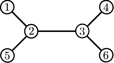


The matroids and are illustrated in the middle of Figure 6.1. The remaining are
Denote by the matroid of the edge between the vertices corresponding to and . The matroid is illustrated by the right picture in Figure 6.1, and the remaining matroids for are isomorphic to . The dimensions of the thin Schubert cells and are
With and , the matroids are -maximal and is -maximal, but is not -maximal. As is not isomorphic to , we see that is smooth and irreducible. Therefore, is smooth and irreducible of dimension 15 by Proposition 3.2, and so is smooth and irreducible by Corollary 2.2.
6.5. Case
There are subdivisions belonging to the set . Given such a combinatorial type , let , and the subcomplex obtained by removing all leaf-vertices of together with their adjacent edges. Set
| (6.2) |
Then
| (6.3) |
Proposition 6.9.
If is smooth and irreducible, then is smooth and irreducible of dimension
| (6.4) |
Proof.
Proposition 6.10.
For any combinatorial type , the subcomplex is vertex-connecting.
Proof.
By Propositions 6.3 and 6.10, the coordinate ring of is isomorphic to . Thus, we need some techniques for determining when a ring of the form is a regular (i.e., its local rings are regular) integral domain. We work in the following more general context. Let with standard basis , let be the variable corresponding to . More generally, let be the monomial corresponding to . Let . Given , let be
Let a finitely generated multiplicative semigroup whose saturation contains the variables , and an ideal generated by distinct nonzero elements ; assume that ( if ). Set . Let be the matrix with rows .
Lemma 6.11.
If, after a permutation of the rows, the matrix has an upper-triangular -submatrix whose diagonal entries equal 1, then is a regular integral domain of Krull dimension .
Proof.
We proceed by induction on . If , then , and the conclusion is clear. Now suppose that the lemma is true for values strictly less than . After permuting the rows and columns (equivalently, permuting the ’s and ’s), we may assume that the first columns form an upper triangular matrix whose diagonal entries equal 1. This means that
Here, is a nonzero constant and the are nonnegative. Therefore, the assignment , and for defines a ring isomorphism
where is the image of under the above substitution. The lemma now follows from the inductive hypothesis. ∎
Lemma 6.11 suffices to determine that is a regular integral domain for most cases in . For the remaining, we use the following Algorithm. Given , denote by the degree of in , i.e., the highest power of appearing in . If , then denote by the coefficient of in . We say that is reduced if has no unit other than elements of as a factor. Because is a unique factorization domain, if is not a unit, then there is a unique expression (up to a factor lying in ) such that and lie in and has no unit (other than an element of ) as a factor.
Algorithm 6.12.
Input: The polynomial ring , a multiplicative semigroup containing all monomials, and a finite set of reduced generators of . Set .
Output: A new presentation of , say , and a finite set of reduced generators of such that
- -
is a polynomial ring on a subset of the
- -
for each and , we have or but .
In particular, if , then is a regular integral domain.
Find and such that and . This means that
for some and such that and . Then perform the substitution followed by a reduction for all elements of , and just the substitution for the elements of ; this produces new sets and . Set . Now repeat this procedure with , and .
Once no such pair exists, this function returns and the presentation .
Proposition 6.13.
If , then is smooth and irreducible of dimension 15.
Proof.
For combinatorial types , there is a presentation of the ideal that satisfies the conditions of Lemma 6.11. So is smooth and irreducible. For the remaining combinatorial types, we apply Algorithm 6.12. In each case, this function returns a presentation of whose ideal is , whence , and therefore , is a regular integral domain. In either case, we get that is smooth and irreducible by Proposition 6.9.
Finally, we compute the dimensions of each using Formula (6.4), verify that each dimension is . ∎
6.6. Case
There are combinatorial types belonging to the set .
Proposition 6.14.
If , then is smooth and irreducible of dimension 15.
Proof.
For any , it happens to be the case that any branch of is a path, and so each of its vertices has 2 or fewer neighbors. For such a vertex , its dual polytope has 2 or fewer internal facets. Thus, each such is smooth and irreducible and the maps from corresponding to the edges adjacent to are SDC-morphisms by Proposition 4.4. By Proposition 3.4, to show that is smooth and irreducible, it suffices to show that is smooth and irreducible. For combinatorial types, there is a presentation of the ideal that satisfies the conditions of Lemma 6.11. For the remaining combinatorial types, we apply Algorithm 6.12, which always returns the ideal . In either case, we see that is a regular integral domain, as required. Finally, we verify that the dimensions of the are all 15 using the formula
which follows from Formula 3.3. ∎
6.7. Case
There are combinatorial types belonging to the set . Similar to the case , given a combinatorial type , let and the subcomplex obtained by removing all leaf-vertices of together with their adjacent edges. Let and be the schemes in Formula 6.2. Formula 6.3 holds, but now cannot be evaluated using a presentation provided by Proposition 6.3 since is not vertex-intersecting.
Recall that a fin is -maximal if there is a such that is -maximal for all . Given a collection of fins of , let be the subcomplex obtained by removing the fins .
Proposition 6.15.
If is smooth and irreducible and each fin is -maximal, then is smooth and irreducible of dimension
| (6.5) |
Proof.
Proposition 6.16.
If , then is smooth and irreducible of dimension 15.
Proof.
Fix , , and the subcomplex obtained by removing all leaf vertices and edges. Let be the set of fins of that have connecting path length 1. We verify that each is -maximal. In this case, the set is vertex-connecting by Proposition 6.2 and vertex-intersecting by hypothesis, and therefore we may compute the coordinate ring of using Proposition 6.3. We verify that these rings are smooth integral domains as in the proof of Proposition 6.13. Finally, we verify that using Formula (6.5). The proposition now follows from Corollary 2.2. ∎
Example 6.17.
Let
The tight span of is given in 6.2. We also see the matroid corresponding to the node of that did not appear in Figure 4.2.


The matroids corresponding to the vertices of are
When and share an edge, the matroid of the edge is denoted by ; in each case, is isomorphic to a matroid of the form . Then Proposition 4.5, and direct computation for the case, tells us the dimensions of the thin Schubert cells corresponding to the vertices and edges of are given by
Moreover, one can check that for the unique fin of . Finally, we compute , to obtain the dimension of . We compute
the ideal is
and is the semigroup of all monomials of . One can check that the condition of Lemma 6.11 does not hold. Thus we apply Algorithm 6.12. That is, we obtain
Observe that with these substitutions, we have , and that the coordinate ring of reduces to . So we have that is smooth, irreducible and of dimension 12.
6.8. Case
There are combinatorial types in . For each combinatorial type , the dual graph has a star-tree subgraph with 4 leaves; the matroid of the center node is isomorphic to , and the matroids of the 4 leaves are isomorphic to either or . The set splits further into 5 groups where if
The sizes of the ’s are
Proposition 6.18.
If , then the limit is smooth and irreducible of dimension .
Proof.
The matroid corresponding to the edge between and is isomorphic to , see Figure 4.2. By Proposition 4.5, the thin Schubert cells , , are smooth, irreducible, and their dimensions are , and
Furthermore, the morphisms are smooth and dominant with connected fibers by Proposition 4.5. The proposition now follows from Proposition 3.2. ∎
Proposition 6.19.
If , then is smooth and irreducible of dimension 15.
Proof.
Suppose , and let . As usual, let be the subcomplex obtained by removing all leaf vertices and edges from . By a direct verification, consists of the tree , and 6 fins, each of which has contact-length 2. In fact, there is a fin attached to at each pair of edges. We verify that each fin is -maximal. Thus is smooth and irreducible by Propositions 3.6 and 4.7. Finally, we verify that using Formula (6.5). The proposition now follows from Corollary 2.2. ∎
Example 6.20.
The vector
represents a combinatorial type in , the tight span is shown in Figure 6.3, together with the matroids corresponding to the nodes of . The tree consists of the vertices , and is smooth and irreducible of dimension 11 by Proposition 6.18. The subcomplex obtained by removing all leaves is obtained by removing the vertex and its adjacent edge. The fins of are:
With and , the fins , , are -maximal, and the fins , , are -maximal. Therefore, is smooth and irreducible by Propositions 3.6 and 4.7. Using this and Proposition 4.5, one may verify that , and therefore is smooth and irreducible by Corollary 2.2.

6.9. Completion of the proofs
The following is a compilation of Propositions 5.1, 6.4, 6.7, 6.13, 6.14, 6.16, 6.19, and Corollary 2.2.
Theorem 6.21.
Suppose .
- (1)
The inverse limit is smooth of dimension 15.
- (2)
If is contained in the relative interior of any cone in the -orbit of , then has 2 connected components. Otherwise, is irreducible.
- (3)
The closed immersion is an isomorphism.
7. The Chow quotient
Recall from the introduction that the diagonal torus of acts on by scaling the coordinates, and this induces an action of the diagonal torus on . This restricts to a free action on , and under the Gelfand-MacPherson correspondence, the quotient coincides with the moduli space of projective-equivalence classes of hyperplanes in in linear general position.
Throughout this section, let be the uniform –matroid. Let be the saturated subgroup from Formula (2.1), and its corresponding torus. Then and the action of on through restricts to the action of on . Thus, we have an inclusion of Chow quotients
By [20], the normalization of the Chow quotient is the toric variety of the pointed fan , where is the secondary fan of .
Recall that is the subfan of whose support is . As is , the closure of in the toric variety coincides with its closure in by [37, Proposition 2.3], and we denote this by . This space has the same normalization as . By Theorem 1.1 and the fact that (where is the image of under the quotient ), we conclude that is schön, and hence is a schön compactification of [27, Theorem 1.5]. In particular, is normal and the boundary is a divisor.
Theorem 7.1.
The log-canonical divisor of is ample. In particular, is the log-canonical compactification of .
Proof.
By [13, Theorem 9.1], it suffices to show that each irreducible stratum is log minimal. As is a schön compactification, its strata are also schön by Formula (7.1) and [28, Corollary 4.2.10]. By [13, Theorem 3.1], a schön very affine variety is log minimal if and only if it is not preserved under translation by a subtorus of . This last property holds if and only if is not preserved under translation by a rational subspace of [21, Lemma 5.2].
Given a cone of , denote by the intersection of with the torus orbit of corresponding to . By [15, Lemma 3.6], there is an isomorphism
| (7.1) |
where is any point in the relative interior of . The fan is convexly disjoint by [33, Proposition 7.9]. This proves that the strata of which are irreducible, i.e., for cones not in the –orbit of by Theorem 1.4, are log minimal. But the strata for in the –orbit of each consists of two disjoint points, which are individually log minimal, as required. ∎
References
- [1] S. Awodey. Category theory, volume 52 of Oxford Logic Guides. Oxford University Press, Oxford, second edition, 2010.
- [2] D. Bendle, J. Boehm, Y. Ren, and B. Schröter. Parallel computation of tropical varieties, their positive part, and tropical Grassmannians, 2020. arXiv:2003.13752.
- [3] J. Bezanson, A. Edelman, S. Karpinski, and V. B. Shah. Julia: A fresh approach to numerical computing. SIAM Review, 59(1):65–98, 2017.
- [4] H. Brenner and S. Schröer. Ample families, multihomogeneous spectra, and algebraization of formal schemes. Pacific J. Math., 208(2):209–230, 2003.
- [5] D. Corey. Initial degenerations of spinor varieties. Preprint, arXiv:2104.03442.
- [6] D. Corey. Initial degenerations of Grassmannians. Sel. Math. New Ser., 27(57), 2021.
- [7] J. A. De Loera, J. Rambau, and F. Santos. Triangulations, volume 25 of Algorithms and Computation in Mathematics. Springer-Verlag, Berlin, 2010. Structures for algorithms and applications.
- [8] C. Eder, W. Decker, C. Fieker, M. Horn, and M. Joswig, editors. The OSCAR book. 2024.
- [9] E. Gawrilow and M. Joswig. polymake: a Framework for Analyzing Convex Polytopes, pages 43–73. Birkhäuser Basel, Basel, 2000.
- [10] I. Gelfand, M. Goresky, R. MacPherson, and V. Serganova. Combinatorial geometries, convex polyhedra, and Schubert cells. Adv. in Math., 63(3):301–316, 1987.
- [11] I. M. Gelfand and R. D. MacPherson. Geometry in Grassmannians and a generalization of the dilogarithm. Adv. in Math., 44(3):279–312, 1982.
- [12] I. M. Gelfand and V. V. Serganova. Combinatorial geometries and the strata of a torus on homogeneous compact manifolds. Uspekhi Mat. Nauk, 42(2(254)):107–134, 287, 1987.
- [13] P. Hacking, S. Keel, and J. Tevelev. Stable pair, tropical, and log canonical compactifications of moduli spaces of del Pezzo surfaces. Invent. Math., 178(1):173–227, 2009.
- [14] R. Hartshorne. Algebraic Geometry. Springer, 1977.
- [15] D. Helm and E. Katz. Monodromy filtrations and the topology of tropical varieties. Canad. J. Math., 64(4):845–868, 2012.
- [16] S. Herrmann. On the facets of the secondary polytope. J. Combin. Theory Ser. A, 118(2):425–447, 2011.
- [17] S. Herrmann, A. Jensen, M. Joswig, and B. Sturmfels. How to draw tropical planes. The Electronic Journal of Combinatorics, 16(2), 2009.
- [18] M. Kaluba, B. Lorenz, and S. Timme. Polymake.jl: A new interface to polymake. In A. M. Bigatti, J. Carette, J. H. Davenport, M. Joswig, and T. de Wolff, editors, Mathematical Software – ICMS 2020, pages 377–385, Cham, 2020. Springer International Publishing.
- [19] M. Kapranov. Chow quotients of Grassmannians. I. In I. M. Gelfand Seminar, volume 16 of Adv. Soviet Math., pages 29–110. Amer. Math. Soc., Providence, RI, 1993.
- [20] M. M. Kapranov, B. Sturmfels, and A. V. Zelevinsky. Quotients of toric varieties. Math. Ann., 290(4):643–655, 1991.
- [21] E. Katz and S. Payne. Realization spaces for tropical fans. In Combinatorial aspects of commutative algebra and algebraic geometry, volume 6 of Abel Symp., pages 73–88. Springer, Berlin, 2011.
- [22] S. Keel and J. McKernan. Contractible extremal rays on . In Handbook of moduli. Vol. II, volume 25 of Adv. Lect. Math. (ALM), pages 115–130. Int. Press, Somerville, MA, 2013.
- [23] S. Keel and J. Tevelev. Geometry of Chow quotients of Grassmannians. Duke Math. J., 134(2):259–311, 2006.
- [24] L. Lafforgue. Chirurgie des grassmanniennes, volume 19 of CRM Monograph Series. American Mathematical Society, Providence, RI, 2003.
- [25] S. H. Lee and R. Vakil. Mnëv-Sturmfels universality for schemes. In A celebration of algebraic geometry, volume 18 of Clay Math. Proc., pages 457–468. Amer. Math. Soc., Providence, RI, 2013.
- [26] M. Luxton. The log canonical compactification of the moduli space of six lines in . ProQuest LLC, Ann Arbor, MI, 2008. Thesis (Ph.D.)–The University of Texas at Austin.
- [27] M. Luxton and Z. Qu. Some results on tropical compactifications. Trans. Amer. Math. Soc., 363(9):4853–4876, 2011.
- [28] D. Maclagan and B. Sturmfels. Introduction to Tropical Geometry, volume 161 of Graduate Studies in Mathematics. American Mathematical Society, Providence, RI, 2015.
- [29] Y. Matsumoto, S. Moriyama, H. Imai, and D. Bremner. Matroid enumeration for incidence geometry. Discrete Comput. Geom., 47(1):17–43, 2012.
- [30] Oscar – open source computer algebra research system, version 0.8.3-dev, 2022.
- [31] J. Oxley. Matroid theory. Oxford Science Publications. The Clarendon Press, Oxford University Press, New York, 1992.
- [32] S. Payne. Fibers of tropicalization. Math. Z., 262(2):301–311, 2009.
- [33] N. Schock. Quasilinear tropical compactifications, 2021. arXiv:2112.02062.
- [34] D. Speyer. Tropical linear spaces. SIAM J. Discrete Math., 22(4):1527–1558, 2008.
- [35] D. Speyer and B. Sturmfels. The tropical Grassmannian. Adv. Geom., 4:389–411, 2004.
- [36] T. Stacks project authors. The stacks project. https://stacks.math.columbia.edu, 2022.
- [37] J. Tevelev. Compactifications of subvarieties of tori. Amer. J. Math., 129(4):1087–1104, 2007.
- [38] R. Vakil. Murphy’s law in algebraic geometry: badly-behaved deformation spaces. Invent. Math., 164(3):569–590, 2006.
- [39] A. N. Varčenko. Newton polyhedra and estimates of oscillatory integrals. Funkcional. Anal. i Priložen., 10(3):13–38, 1976.
- [40] A. N. Varčenko. Zeta-function of monodromy and Newton’s diagram. Invent. Math., 37(3):253–262, 1976.