Interferometric Hi intensity mapping: perturbation theory predictions and foreground removal effects2022Interferometric Hi intensity mapping: perturbation theory predictions and foreground removal effects–10
Abstract
We provide perturbation theory predictions for the Hi intensity mapping power spectrum multipoles using the Effective Field Theory of Large Scale Structure (EFTofLSS), which should allow us to exploit mildly nonlinear scales. Assuming survey specifications typical of proposed interferometric Hi intensity mapping experiments like CHORD and PUMA, and realistic ranges of validity for the perturbation theory modelling, we run mock full shape MCMC analyses at , and compare with Stage-IV optical galaxy surveys. We include the impact of 21cm foreground removal using simulations-based prescriptions, and quantify the effects on the precision and accuracy of the parameter estimation. We vary 11 parameters in total: 3 cosmological parameters, 7 bias and counterterms parameters, and the Hi brightness temperature. Amongst them, the 4 parameters of interest are: the cold dark matter density, , the Hubble parameter, , the primordial amplitude of the power spectrum, , and the linear Hi bias, . For the best case scenario, we obtain unbiased constraints on all parameters with errors at confidence level. When we include the foreground removal effects, the parameter estimation becomes strongly biased for , and , while is less biased (). We find that scale cuts are required to return accurate estimates for and , at the price of a decrease in the precision, while remains strongly biased. We comment on the implications of these results for real data analyses.
Keywords:
cosmology: theory – cosmology: observations – large-scale structure of the Universe – methods:statistical1 Introduction
Over the next few years, observations of the redshifted 21cm line emission from neutral hydrogen gas (Hi) with a new generation of radio telescopes can push the boundaries of our understanding of cosmology and galaxy evolution. Remarkably, Hi surveys can trace the matter distribution from the present time () to the Epoch of Reionization () and beyond, mapping a large part of the observable volume of the Universe.
In the meantime, spectroscopic optical galaxy surveys have already proven extremely successful at mapping the low redshift Universe, and providing exquisite constraints on dark energy and gravity (Mueller et al. 2018; Alam et al. 2021, see, for example,). These surveys operate by detecting galaxies in 3D, i.e., by measuring the redshift and angular position of each galaxy very precisely. In the radio wavelengths, due to the weakness of the Hi signal, being competitive with optical galaxy surveys using the traditional approach of detecting individual galaxies is extremely challenging. This challenge gave rise to an alternative observational technique, dubbed Hi intensity mapping, which maps the entire Hi flux coming from many galaxies together in 3D voxels. (Battye et al. 2004; Chang et al. 2008; Peterson et al. 2009; Seo et al. 2010; Ansari et al. 2012). Provided several observational challenges and systematic effects are mitigated or controlled, the Hi intensity mapping method has the potential to provide detailed maps of the Universe back to 1 billion years after the Big Bang (Ahmed et al. 2019; Kovetz et al. 2020; Moresco et al. 2022).
A number of Hi intensity mapping experiments are expected to come online over the coming years, with some of them already taking data with pilot surveys. Examples are the proposed MeerKLASS survey using the South African MeerKAT array (Santos et al. 2017), FAST (Hu et al. 2020), CHIME (Bandura et al. 2014), HIRAX (Newburgh et al. 2016; Crichton et al. 2022), Tianlai (Li et al. 2020; Wu et al. 2021), PUMA (Slosar et al. 2019), and CHORD (Vanderlinde et al. 2019). Pathfinder surveys with the Green Bank Telescope (GBT), Parkes, CHIME, and MeerKAT, have achieved detections of the cosmological 21 cm emission, but have relied on cross-correlation analyses with optical galaxy surveys (Chang et al. 2010; Masui et al. 2013; Anderson et al. 2018; Wolz et al. 2022; Amiri et al. 2022a; Cunnington et al. 2022).
A major challenge for the Hi intensity mapping method is the presence of strong astrophysical emission: 21cm foregrounds such as galactic synchrotron (Zheng et al. 2017), point sources, and free-free emission, contaminate the maps and can be orders of magnitude stronger than the cosmological Hi signal (Oh & Mack 2003). Hence, they have to be removed. We can differentiate these dominant foregrounds from the signal taking advantage of their spectral smoothness (Liu & Tegmark 2011; Chapman et al. 2012; Wolz et al. 2014; Shaw et al. 2015; Alonso et al. 2015; Cunnington et al. 2020). As an example, 21cm foreground removal studies using low redshift Hi intensity mapping simulations and real data employ blind foreground removal techniques like Principal Component Analysis (PCA) (Switzer et al. 2013; Switzer et al. 2015; Alonso et al. 2015) or Independent Component Analysis (Hyvärinen 1999; Wolz et al. 2017). The procedure of foreground removal results in Hi signal loss, removing power from modes along the parallel and perpendicular to the line-of-sight (LoS) directions, with the parallel to the LoS effect being more severe than the perpendicular one (Witzemann et al. 2019; Cunnington et al. 2020).
The aim of this work is to investigate the systematic biases from 21cm foreground removal assuming state-of-the-art interferometric Hi intensity mapping experiments. To quantify how these systematic biases propagate on the cosmological parameter estimation, we will model the Hi signal using perturbation theory and run full shape MCMC analyses on synthetic data contaminated with 21cm foreground removal effects. We will also benchmark our predictions against a “Stage-IV” spectroscopic optical galaxy survey like DESI (Aghamousa et al. 2016) or Euclid (Laureijs et al. 2011; Blanchard et al. 2020).
The paper is organised as follows: In section 2 we present the perturbation theory model we will use. In section 3 we produce our synthetic mock data and contaminate them with simulated 21cm foreground removal effects. We present the results of our full shape MCMC runs in section 4. In section 5 we summarise our findings and conclude.
2 Theoretical modelling
Our observable is the Hi power spectrum multipoles, and we follow the formalism used in optical galaxy surveys analyses. Similarly to optical galaxies, redshift space distortions (RSDs) introduce anisotropies in the observed Hi power spectrum. In order to account for this, we consider the 3D power spectrum as a function of redshift , , and , where is the amplitude of the wave vector and the cosine of the angle between the wave vector and the LoS component. This gives and .
Before we present the 1-loop perturbation theory model we will use, it is useful to discuss linear theory. We can model RSDs by considering the Kaiser effect (Kaiser 1987), which is a large-scale effect dependent on the growth rate, . To linear order, the anisotropic Hi power spectrum can be written as:
| (1) |
Here, is the underlying matter power spectrum, is the (linear) Hi bias, and is the mean Hi brightness temperature. is the thermal noise of the telescope and is the shot noise, , where is the number density of objects. The contribution is expected to be subdominant (smaller than the thermal noise of the telescope) and is usually neglected (Villaescusa-Navarro et al. 2018). The noise power spectrum for a typical interferometer is given by (Zaldarriaga et al. 2004; Bull et al. 2015):
| (2) |
Here, is the effective beam area, , is the comoving distance to the observation redshift , and with MHz. is the system temperature, is the survey area, and is the total observing time.
The antennae distribution function can be calculated using a fitting formula (Ansari et al. 2018). For a square array with receivers, the number of baselines as a function of physical distance of antennas is given by
| (3) |
where , , and the -plane density is
| (4) |
The Hi abundance and clustering properties have been studied using simulations and semi-analytical modeling (Padmanabhan et al. 2017; Villaescusa-Navarro et al. 2018; Spinelli et al. 2020, see, e.g.,). The clustering of Hi should be accurately described by perturbative methods at mildly nonlinear scales (Sarkar et al. 2016; McQuinn & D’Aloisio 2018; Sarkar & Bharadwaj 2019; Castorina & White 2019; Sailer et al. 2021; Karagiannis et al. 2022; Qin et al. 2022). Modelling nonlinear scales is necessary in order to get precise and accurate cosmological constraints with instruments like HIRAX, CHIME, CHORD, and PUMA, and it also helps break degeneracies, for example between and the primordial power spectrum amplitude, . Similar degeneracies exist for , which is proportional to the Hi mean density, . Accurate () measurements of are available at low redshifts (Crighton et al. 2015), and it can also be constrained by joint analyses of different probes (Obuljen et al. 2018; Chen et al. 2019) or by exploiting very small scales that can be described using bespoke Hi halo models (Chen et al. 2021).
In this work we will use the “EFTofLSS” formalism that has been developed to model the power spectrum multipoles of biased tracers in redshift space. The main difference between this model and the standard 1-loop Standard Perturbation Theory (SPT) formalism (Bernardeau et al. 2002) is that the EFTofLSS approach accounts for the impact of nonlinearities on mildly nonlinear scales by introducing effective stresses in the equations of motion. This results in the addition of counterterms to the 1-loop power spectrum, which represent the effects of short distance physics at long distances.
The EFTofLSS model we will employ is described in various papers (see e.g. Perko et al. 2016 and references therein), and we refer to D’Amico et al. 2020 for its application to the DR12 BOSS data. Main assumptions are that we live in a spatially expanding, homogeneous and isotropic background spacetime, and that we work on sub-horizon scales with ( where and are the density and velocity perturbations, respectively).
The 1-loop redshift space galaxy power spectrum then reads (Perko et al. 2016; D’Amico et al. 2020):
| (5) |
where /Mpc and is the mean galaxy density. The various terms are summarised nicely in Nishimichi et al. 2020, and we follow this description here: the term represents a combination of a higher derivative bias and the speed of sound of dark matter; the terms represent the redshift-space counterterms, while the terms represent the stochastic counterterms. The kernels , , and are the redshift-space galaxy density kernels appearing in the 1-loop power spectra. They are expressed in terms of the galaxy density and velocity kernels and 4 bias parameters: {}. For flat CDM, which we will assume in this work, the logarithmic growth rate is calculated by solving for the linear growth factor (with the scale factor), and yields:
The model of Equation 5 has recently been implemented in a publicly available Python code, PyBird (D’Amico et al. 2021). In principle, the model can describe any biased tracer of matter, so we can straightforwardly apply it to Hi. Following the literature we perform the following changes of variables: , , , , and also fix so that our final set of nuisance parameters is: . We will comment on these choices when we construct our mock data in section 3.
The cosmological parameters that the code takes as input are: the cold dark matter density , the baryonic matter density , the Hubble parameter , the amplitude of the primordial power spectrum, , and the scalar spectral index, . We will describe the code and other software we used to speed-up the parameter inference in more detail in section 4.
3 Mock data
For our analysis we produce synthetic Hi monopole and quadrupole data running Pybird for a central redshift . We will not use the hexadecapole as it is not expected to add significant cosmological information, and it is more affected by nonlinear uncertainties. In addition, as shown in Cunnington et al. 2020; Soares et al. 2021, the Hi intensity mapping hexadecapole (as well as higher order multipoles) can be used for identifying the effects of foreground removal and other systematics. Not using the hexadecapole allows us to set . The choice is motivated by the assumption that the functions multiplying and are too small to affect the results. These assumptions follow the BOSS data analyses choices (D’Amico et al. 2020), but they will need to be reaffirmed with bespoke Hi simulations and real data. The fiducial cosmological parameters are (Aghanim et al. 2020):
For setting the fiducial values of the nuisance parameters, we perform fits to Hi intensity mapping simulations. These are described in Appendix A, and we find:
We remark that the value of the linear Hi bias is in very good agreement with values found at similar redshifts in other works (Sarkar et al. 2016; Villaescusa-Navarro et al. 2018). We also note that in all our MCMC forecasts we will marginalise over the nuisance parameters.
The model in Equation 5 has to be rescaled by the square of the Hi brightness temperature, , which in turn depends on the Hi abundance, . Using the fitting function from SKA Cosmology SWG et al. 2020 we set as our fiducial value for this parameter.
We also need a data covariance. To calculate this we will assume an ambitious CHORD-like intensity mapping survey (Vanderlinde et al. 2019). CHORD (Canadian Hydrogen Observatory and Radio transient Detector) is a successor to CHIME (Amiri et al. 2022b), aiming to perform a very large sky Hi intensity mapping survey. Its core array consists of 512 dishes, each 6m in diameter. The bandwidth is large, covering the 300-1500 MHz band, or redshifts up to . We will assume K in our forecasts. Another very ambitious proposal is PUMA, a close-packed interferometer array with 32,000 dishes, covering the frequency range 200-1100 MHz, or redshifts (Slosar et al. 2019). We expect both of these instruments to be able to achieve similar signal-to-noise ratios (), and we will focus on CHORD from now on.
Aiming to establish how CHORD can complement and compete with state-of-the-art optical galaxy surveys, we choose a low redshift bin centred at with width . Our fiducial CHORD-like survey covers on the sky, resulting in a survey bin volume . We assume a hrs survey and calculate the noise power spectrum using Equation 2, with the fitting parameters needed in Equation 4 being (Ansari et al. 2018). The corresponding baseline density for our CHORD-like array is shown in Figure 1 (see Appendix A of Karagiannis et al. 2022 for the case of a HIRAX-like array).
We can now calculate for our CHORD-like survey using Equation 2. Dividing by and inverting, we can define an effective mean number density . For a Stage-IV spectroscopic galaxy survey like DESI (Aghamousa et al. 2016) or Euclid (Laureijs et al. 2011; Blanchard et al. 2020), the shot noise is the inverse of the number density of galaxies, . In Figure 2 we plot the signal-to-noise-ratio (squared) for the power spherically averaged power spectrum (the monopole, ) for different surveys. Stage-IV corresponds to a spectroscopic optical galaxy survey with . “CHORD-optimal” corresponds to an idealised case for an interferometric Hi intensity mapping survey without any systematic effects, while “CHORD-with-sys” illustrates the case where sensitivity is lost at small (see also Fig. 15 in (Ansari et al. 2018)). This can be due to foreground removal effects which mainly affect the small , and/or inability to probe the small due to baseline restrictions. For the case of the CHORD-like survey at , this can result to loss of sensitivity in a range , and we will consider different scale cuts in our forecasts to take this into account. In all cases, Figure 2 demonstrates that a CHORD-like experiment can achieve a higher signal-to-noise-ratio in the nonlinear regime, compared to a Stage-IV optical galaxy survey.
We can now proceed to calculate the multipole covariances analytically, using the Gaussian approximation (Taruya et al. 2010; Soares et al. 2021). We present the resulting mock data and measurement errors in Figure 3 for the CHORD-optimal case. We notice that in the case of the monopole the error bars are not large enough to be visible. At this low redshift, and with such high , nonlinear uncertainties are expected to become important at a relatively low . Hence, we choose the range of validity for the EFTofLSS modelling to be Mpc (this should be a good assumption, but it has to be validated with tailored Hi simulations for these experiments). We are now ready to perform MCMC forecasts.
4 MCMC analyses
To calculate posterior distributions on the parameters we have run MCMCs using the ensemble slice sampling codes emcee (Foreman-Mackey et al. 2013) and zeus (Karamanis et al. 2021). The latter has been recently used to run mock full shape MCMC analyses assuming galaxy surveys specifications using the Matryoshka suite of neural network based emulators (Donald-McCann et al. 2021; Donald-McCann et al. 2022). Due to the impressive increase in computational speed for the inference ( orders of magnitude improvement with respect to the PyBird runs), we opted for this setup to run and present our final MCMC forecasts11 1 An alternative approach to speed-up the inference is to use a fast and accurate linear matter power spectrum emulator such as bacco (Aricò et al. 2021) or CosmoPower (Spurio Mancini et al. 2022) as input in a perturbation theory code, instead of running a Boltzmann solver like CAMB (Lewis et al. 2000) or CLASS (Lesgourgues 2011; Blas et al. 2011). . We vary three cosmological parameters, , seven bias and counterterms parameters, , and, in the case of IM, we also vary . The scalar spectral index is fixed to its true value, and so is the baryon fraction .
For the 3 cosmological parameters and , we assume the uniform flat priors shown in Table 1. We do not employ Planck priors on because we wish to assess the precision vs accuracy performance of interferometric Hi intensity mapping independently of CMB experiments. For we take a flat prior . For the rest of the bias and counterterms parameters, we follow D’Amico et al. 2020 and set:
Finally, we assume a Gaussian likelihood given by:
| (6) |
with being the mock data (the power spectrum monopole, , and quadrupole, ), being the EFTofLSS model predictions for a given set of parameters, , and being the covariance matrix.
4.1 The systematics-free, Stage-IV survey scenario
We start by comparing the performance of a Stage-IV spectroscopic galaxy survey and an analogous intensity mapping survey, assuming both of them are free of systematic effects. The volumes of the surveys are taken to be exactly the same22 2 Hi intensity mapping surveys can cover a much wider redshift range compared to spectroscopic optical galaxy surveys, but our goal here is to compare their performance on a given redshift bin., but the effective mean number densities (i.e., the noise components) are different as we have described in detail in section 3 (see e.g. Figure 2). Following up on the discussion in the previous section, we emphasise again that in the case of Hi intensity mapping there is an additional overall amplitude parameter, , which we vary. This means that a total of 10 (11) parameters are varied in the MCMC for the optical (IM) surveys under consideration.
The MCMC contours for the idealised case are shown in Figure 4. We are able to recover the true values in an unbiased manner, which also confirms the accuracy of the Matryoshka emulator (see Donald-McCann et al. 2022 for a suite of validation tests). The Stage-IV spectroscopic optical galaxy survey and the CHORD-like Hi intensity mapping survey have similar constraining power when the same survey volume is assumed. An exception is the primordial amplitude . In the CHORD-like IM case, additional degeneracies due to varying increase the uncertainty in compared to the optical case.
From Table 1 we see that, in the absence of systematics, the CHORD-like Hi intensity mapping survey determines with error, with error, with error, and (the linear Hi bias) with error. The survey can also constrain , demonstrating how exploiting mildly nonlinear scales can break degeneracies.
4.2 Contaminating the data vector with 21cm foreground removal effects
In order to contaminate our synthetic data vector (i.e., the Hi power spectrum multipoles and in Figure 3) with 21cm foreground removal effects, we will use the simulations-based prescription by Soares et al. 2021. This prescription can fit Hi intensity mapping simulations with foreground removal effects, assuming that PCA or FastICA with independent components was used for the foreground cleaning. The choice corresponds to an excellent calibration scenario (which will hopefully be the case by the time CHORD and PUMA come online) and no polarization leakage (Wolz et al. 2014; Alonso et al. 2015; Liu & Shaw 2020; Cunnington et al. 2021). For existing Hi intensity mapping surveys, we know that much more aggressive foreground removal (much higher ) is employed to deal with more complicated foregrounds, noise, and unknown systematics (see e.g. Switzer et al. 2013; Masui et al. 2013; Wolz et al. 2022; Cunnington et al. 2022).
We present the result of contaminating our data vector with 21cm foreground removal effects in Figure 5. This is our mock data vector for the remainder of the paper.
As we can see, foreground cleaning results in the damping of power across a wide range of scales in the spherically averaged power spectrum (the monopole, ). This is a well known effect, which has also been identified in the context of high redshift 21cm surveys of the Epoch of Reionization (Petrovic & Oh 2011). Higher order multipoles were first studied extensively in Blake 2019; Cunnington et al. 2020; Soares et al. 2021, focusing on post-reionization Hi. In the case of the quadrupole (), where is weighted as a function of , we see an enhancement of power on large scales. It is also important to note that, both for and , while the largest effect is clearly on small , there is still an effect along larger . Given that the error bars of our chosen surveys are extremely small, the large effect may introduce a significant systematic bias as well. We can only verify and quantify this at the level of the parameter inference, and we will do so in the following sections.
We remark that we assume no prior knowledge of the 21cm foreground removal fitting function from Soares et al. 2021. That is, we will not attempt to include a model (and associated nuisance parameters we need to vary) for the 21cm foreground removal effects in our theory vector. We will instead follow a more conservative, “data-driven” approach, imposing scale cuts on the contaminated data vector. However, the former method has been shown to be very promising in the context of single-dish experiments, and it would be important to re-evaluate its performance when realistic, end-to-end simulations are available (see e.g. the discussion in Spinelli et al. 2022).
Finally, before presenting our MCMC analyses using the contaminated data vector, it is instructive to see how varying our 4 parameters of interest affects the predictions of the EFTofLSS model of Equation 5, and compare with the features of the 21cm foreground removal effects. This comparison is shown in Figure 6.
It is well known that different cosmological and nuisance parameters affect the power spectrum amplitude and shape in distinct ways. Comparing these with our simulated 21cm foreground removal effects suggests that some parameters, for example , have features on the mildly nonlinear scales that might make them easier to constrain in an unbiased way (i.e., to disentangle them from the foreground removal effects) than others, for example and .
4.3 Imposing cuts: precision vs accuracy
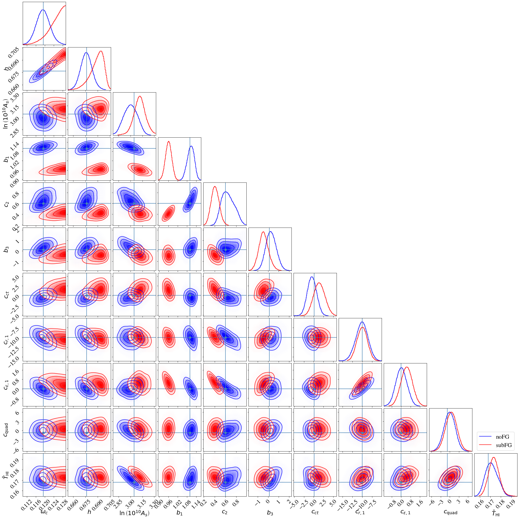
In this section we perform an MCMC analysis for the CHORD-like survey under consideration, using the contaminated Hi intensity mapping data vector with different limits. Our results for the 4 parameters of interest are summarised in Table 1 and Figure 7. The different scale cuts we consider are the following:
- •
Case I: We start by imposing a scale cut in order to exclude the largest scales where foreground subtraction has the most impact. This is not enough: the parameter estimation becomes strongly biased for , and . The primordial amplitude is unbiased within because of the marginalisation of (i.e., if was kept fixed, would also be strongly biased). For the Hi brightness temperature we get: .
- •
Case II: Imposing a stricter scale cut . In this case the , , and parameters are unbiased within , while remains biased. For the Hi brightness temperature we get: .
- •
Case III: Imposing a scale cut . In this case the , , and parameters are unbiased within , while remains biased. For the Hi brightness temperature we get: .
In Figure 8 we compare the idealised case (noFG) and the cases with limits that lead to unbiased (within ) constraints on , , and . Looking back at Figure 6, we deduce that for the scale-dependent features of varying and are sufficient to constrain them accurately, in contrast to , which gets significantly biased due to the amplitude change from the 21cm foreground removal. The primordial amplitude is less affected because of the marginalisation of (we have checked that when is kept fixed, becomes strongly biased).
From Table 1, Figure 7 and Figure 8 we also see that the price to pay for the unbiased estimates of and parameters is a decrease in the precision with respect to the idealised case, as expected.
5 Conclusions
We have provided perturbation theory predictions for Hi intensity mapping, and performed full shape MCMC analyses including the impact of 21cm foreground removal. Albeit our framework was developed in the context of low-redshift, interferometric Hi intensity mapping surveys like CHIME, HIRAX, CHORD, and PUMA, our results are also relevant for single-dish surveys as well as Epoch of Reionization surveys. The main conclusions we draw from this work are:
- •
In the idealised case without any systematic biases in the data, interferometric Hi intensity mapping surveys with instruments like CHORD and PUMA are competitive with Stage-IV optical galaxy surveys. Our results, summarised in Table 1, assume a single redshift bin centred at . In the case of redshift-independent parameters like , and , we naively expect the parameter estimation uncertainties to be reduced by roughly , where is the number of redshift bins. This is an advantage for Hi intensity mapping surveys with respect to optical surveys, since the former are not shot-noise limited and can rapidly cover very large redshift ranges. However, the thermal noise of an interferometer can increase rapidly with redshift. Nevertheless, forecasts for experiments similar to what we consider here have shown that interferometric Hi intensity mapping should be advantageous at high redshift . The cosmological volume spanned at this range is three times higher than the typical optical galaxy surveys range, , with an increased , i.e., an increased number of (easier to model) linear and mildly nonlinear modes. Forecasts for a dedicated “Stage-II” Hi intensity mapping experiment showed that is achievable for all modes with at (Ansari et al. 2018).
- •
Including 21cm foreground removal effects based on simulations-based prescriptions, the parameter estimation becomes strongly biased for , and , while is less biased ().
- •
Adopting the scale cuts approach to try and mitigate the biases, we find that scale cuts are required to return accurate estimates for and , at the price of a decrease in the precision, while remains biased.
In future work it would be interesting to investigate the possible Hi and cosmology dependence of the foreground transfer function. This is a method to correct for signal loss from foreground removal, which has been used in all the Hi-galaxy cross-correlation detections so far. Due to the low of current experiments, the cosmology is kept fixed to the Planck best-fit values and the only parameter we can constrain is , with the Hi-galaxy cross-correlation coefficient (Masui et al. 2013; Anderson et al. 2018; Wolz et al. 2022; Cunnington et al. 2022). The foreground transfer function is constructed using mock simulations with fixed Hi and cosmological parameters. In light of our results, we believe it is important to study how robust the transfer function construction (and the resulting Hi signal loss correction) is with respect to varying the parameters in the mock simulations.
| Parameters of interest | |||||
|---|---|---|---|---|---|
| Fiducial values | 0.1193 | 0.677 | 3.047 | 1.1 | |
| Priors | [0.101,0.140] | [0.575,0.748] | [2.78,3.32] | [0,4] | |
| Case | -range [Mpc] | ||||
| Optical galaxy survey (Figure 4) | |||||
| IM-noFG (Figure 4) | |||||
| IM-subFG, (Figure 7) | |||||
| IM-subFG, (Figure 7 and Figure 8) | |||||
| IM-subFG, (Figure 7 and Figure 8) |
Acknowledgements
I acknowledge use of open source software: Python (Van Rossum & Drake Jr 1995; Hunter 2007), numpy (Van Der Walt et al. 2011), scipy (Virtanen et al. 2020), TensorFlow (Abadi et al. 2015), astropy (Astropy Collaboration et al. 2018), corner (Foreman-Mackey 2016), GetDist (Lewis 2019). I thank New Mexico State University (USA) and Instituto de Astrofisica de Andalucia CSIC (Spain) for hosting the Skies & Universes site for cosmological simulation products. My research is funded by a UK Research and Innovation Future Leaders Fellowship [grant MR/S016066/1]. For the purpose of open access, the author has applied a Creative Commons Attribution (CC BY) licence to any Author Accepted Manuscript version arising from this submission.
Data Availability
The data products will be shared on reasonable request to the corresponding author.
References
- Abadi et al. (2015) Abadi M., et al., 2015, TensorFlow: Large-Scale Machine Learning on Heterogeneous Systems, https://www.tensorflow.org/
- Ade et al. (2016) Ade P. A. R., et al., 2016, Astron. Astrophys., 594, A13
- Aghamousa et al. (2016) Aghamousa A., et al., 2016, The DESI Experiment Part I: Science,Targeting, and Survey Design (arXiv:1611.00036)
- Aghanim et al. (2020) Aghanim N., et al., 2020, Astron. Astrophys., 641, A6
- Ahmed et al. (2019) Ahmed Z., et al., 2019, arXiv e-prints, p. arXiv:1907.13090
- Alam et al. (2021) Alam S., et al., 2021, Phys. Rev. D, 103, 083533
- Alonso et al. (2015) Alonso D., Bull P., Ferreira P. G., Santos M. G., 2015, Mon. Not. Roy. Astron. Soc., 447, 400
- Amiri et al. (2022b) Amiri M., et al., 2022b, An Overview of CHIME, the Canadian Hydrogen Intensity Mapping Experiment (arXiv:2201.07869)
- Amiri et al. (2022a) Amiri M., et al., 2022a, Detection of Cosmological 21 cm Emission with the Canadian Hydrogen Intensity Mapping Experiment (arXiv:2202.01242)
- Anderson et al. (2018) Anderson C., et al., 2018, MNRAS, 476, 3382
- Ansari et al. (2012) Ansari R., et al., 2012, Astron. Astrophys., 540, A129
- Ansari et al. (2018) Ansari R., et al., 2018, Inflation and Early Dark Energy with a Stage II Hydrogen Intensity Mapping experiment (arXiv:1810.09572)
- Aricò et al. (2021) Aricò G., Angulo R. E., Zennaro M., 2021, Accelerating Large-Scale-Structure data analyses by emulating Boltzmann solvers and Lagrangian Perturbation Theory (arXiv:2104.14568)
- Astropy Collaboration et al. (2018) Astropy Collaboration et al., 2018, AJ, 156, 123
- Bandura et al. (2014) Bandura K., et al., 2014, Proc. SPIE Int. Soc. Opt. Eng., 9145, 22
- Battye et al. (2004) Battye R. A., Davies R. D., Weller J., 2004, Mon. Not. Roy. Astron. Soc., 355, 1339
- Bernardeau et al. (2002) Bernardeau F., Colombi S., Gaztanaga E., Scoccimarro R., 2002, Phys. Rept., 367, 1
- Blake (2019) Blake C., 2019, Mon. Not. Roy. Astron. Soc., 489, 153
- Blanchard et al. (2020) Blanchard A., et al., 2020, Astron. Astrophys., 642, A191
- Blas et al. (2011) Blas D., Lesgourgues J., Tram T., 2011, JCAP, 07, 034
- Bull et al. (2015) Bull P., Ferreira P. G., Patel P., Santos M. G., 2015, Astrophys. J., 803, 21
- Castorina & White (2019) Castorina E., White M., 2019, JCAP, 06, 025
- Chang et al. (2008) Chang T.-C., Pen U.-L., Peterson J. B., McDonald P., 2008, Phys. Rev. Lett., 100, 091303
- Chang et al. (2010) Chang T.-C., Pen U.-L., Bandura K., Peterson J. B., 2010, Nature, 466, 463
- Chapman et al. (2012) Chapman E., et al., 2012, Mon. Not. Roy. Astron. Soc., 423, 2518
- Chen et al. (2019) Chen S.-F., Castorina E., White M., Slosar A., 2019, JCAP, 07, 023
- Chen et al. (2021) Chen Z., Wolz L., Spinelli M., Murray S. G., 2021, Mon. Not. Roy. Astron. Soc., 502, 5259
- Crichton et al. (2022) Crichton D., et al., 2022, J. Astron. Telesc. Instrum. Syst., 8, 011019
- Crighton et al. (2015) Crighton N. H., et al., 2015, Mon. Not. Roy. Astron. Soc., 452, 217
- Croton et al. (2016) Croton D. J., et al., 2016, Astrophys. J. Suppl., 222, 22
- Cunnington et al. (2020) Cunnington S., Pourtsidou A., Soares P. S., Blake C., Bacon D., 2020, Mon. Not. Roy. Astron. Soc., 496, 415
- Cunnington et al. (2021) Cunnington S., Irfan M. O., Carucci I. P., Pourtsidou A., Bobin J., 2021, Mon. Not. Roy. Astron. Soc., 504, 208
- Cunnington et al. (2022) Cunnington S., et al., 2022, HI intensity mapping with MeerKAT: power spectrum detection in cross-correlation with WiggleZ galaxies (arXiv:2206.01579)
- D’Amico et al. (2020) D’Amico G., Gleyzes J., Kokron N., Markovic K., Senatore L., Zhang P., Beutler F., Gil-Marín H., 2020, JCAP, 05, 005
- D’Amico et al. (2021) D’Amico G., Senatore L., Zhang P., 2021, JCAP, 01, 006
- Donald-McCann et al. (2021) Donald-McCann J., Beutler F., Koyama K., Karamanis M., 2021, matryoshka: Halo Model Emulator for the Galaxy Power Spectrum (arXiv:2109.15236), doi:10.1093/mnras/stac239
- Donald-McCann et al. (2022) Donald-McCann J., Koyama K., Beutler F., 2022, matryoshka II: Accelerating Effective Field Theory Analyses of the Galaxy Power Spectrum (arXiv:2202.07557)
- Foreman-Mackey (2016) Foreman-Mackey D., 2016, The Journal of Open Source Software, 1, 24
- Foreman-Mackey et al. (2013) Foreman-Mackey D., Hogg D. W., Lang D., Goodman J., 2013, Publ. Astron. Soc. Pac., 125, 306
- Hu et al. (2020) Hu W., Wang X., Wu F., Wang Y., Zhang P., Chen X., 2020, Mon. Not. Roy. Astron. Soc., 493, 5854
- Hunter (2007) Hunter J. D., 2007, Computing In Science & Engineering, 9, 90
- Hyvärinen (1999) Hyvärinen A., 1999, IEEE transactions on neural networks, 10 3, 626
- Kaiser (1987) Kaiser N., 1987, Mon. Not. Roy. Astron. Soc., 227, 1
- Karagiannis et al. (2022) Karagiannis D., Maartens R., Randrianjanahary L. F., 2022, JCAP, 11, 003
- Karamanis et al. (2021) Karamanis M., Beutler F., Peacock J. A., 2021, Mon. Not. Roy. Astron. Soc., 508, 3589
- Klypin et al. (2016) Klypin A., Yepes G., Gottlober S., Prada F., Hess S., 2016, Mon. Not. Roy. Astron. Soc., 457, 4340
- Knebe et al. (2018) Knebe A., et al., 2018, Mon. Not. Roy. Astron. Soc., 474, 5206
- Kovetz et al. (2020) Kovetz E. D., et al., 2020, Bull. Am. Astron. Soc., 51, 101
- Laureijs et al. (2011) Laureijs R., et al., 2011, Euclid Definition Study Report (arXiv:1110.3193)
- Lesgourgues (2011) Lesgourgues J., 2011, The Cosmic Linear Anisotropy Solving System (CLASS) I: Overview (arXiv:1104.2932)
- Lewis (2019) Lewis A., 2019, GetDist: a Python package for analysing Monte Carlo samples (arXiv:1910.13970)
- Lewis et al. (2000) Lewis A., Challinor A., Lasenby A., 2000, Astrophys. J., 538, 473
- Li et al. (2020) Li J., et al., 2020, Sci. China Phys. Mech. Astron., 63, 129862
- Liu & Shaw (2020) Liu A., Shaw J. R., 2020, Publ. Astron. Soc. Pac., 132, 062001
- Liu & Tegmark (2011) Liu A., Tegmark M., 2011, Phys. Rev. D, 83, 103006
- Masui et al. (2013) Masui K. W., et al., 2013, Astrophys. J., 763, L20
- McQuinn & D’Aloisio (2018) McQuinn M., D’Aloisio A., 2018, JCAP, 10, 016
- Moresco et al. (2022) Moresco M., et al., 2022, Unveiling the Universe with Emerging Cosmological Probes (arXiv:2201.07241)
- Mueller et al. (2018) Mueller E.-M., Percival W., Linder E., Alam S., Zhao G.-B., Sánchez A. G., Beutler F., Brinkmann J., 2018, Mon. Not. Roy. Astron. Soc., 475, 2122
- Newburgh et al. (2016) Newburgh L., et al., 2016, Proc. SPIE Int. Soc. Opt. Eng., 9906, 99065X
- Nishimichi et al. (2020) Nishimichi T., D’Amico G., Ivanov M. M., Senatore L., Simonović M., Takada M., Zaldarriaga M., Zhang P., 2020, Phys. Rev. D, 102, 123541
- Obuljen et al. (2018) Obuljen A., Castorina E., Villaescusa-Navarro F., Viel M., 2018, JCAP, 05, 004
- Oh & Mack (2003) Oh S. P., Mack K. J., 2003, Mon. Not. Roy. Astron. Soc., 346, 871
- Padmanabhan et al. (2017) Padmanabhan H., Refregier A., Amara A., 2017, Mon. Not. Roy. Astron. Soc., 469, 2323
- Perko et al. (2016) Perko A., Senatore L., Jennings E., Wechsler R. H., 2016, Biased Tracers in Redshift Space in the EFT of Large-Scale Structure (arXiv:1610.09321)
- Peterson et al. (2009) Peterson J. B., et al., 2009, in astro2010: The Astronomy and Astrophysics Decadal Survey. p. 234 (arXiv:0902.3091)
- Petrovic & Oh (2011) Petrovic N., Oh S. P., 2011, Monthly Notices of the Royal Astronomical Society, 413, 2103
- Qin et al. (2022) Qin W., Schutz K., Smith A., Garaldi E., Kannan R., Slatyer T. R., Vogelsberger M., 2022, An Effective Bias Expansion for 21 cm Cosmology in Redshift Space (arXiv:2205.06270)
- SKA Cosmology SWG et al. (2020) SKA Cosmology SWG et al., 2020, Publ. Astron. Soc. Austral., 37, e007
- Sailer et al. (2021) Sailer N., Castorina E., Ferraro S., White M., 2021, JCAP, 12, 049
- Santos et al. (2017) Santos M. G., et al., 2017, in MeerKAT Science: On the Pathway to the SKA. (arXiv:1709.06099)
- Sarkar & Bharadwaj (2019) Sarkar D., Bharadwaj S., 2019, Mon. Not. Roy. Astron. Soc., 487, 5666
- Sarkar et al. (2016) Sarkar D., Bharadwaj S., Anathpindika S., 2016, Monthly Notices of the Royal Astronomical Society, 460, 4310
- Seo et al. (2010) Seo H.-J., Dodelson S., Marriner J., Mcginnis D., Stebbins A., Stoughton C., Vallinotto A., 2010, Astrophys. J., 721, 164
- Shaw et al. (2015) Shaw J. R., Sigurdson K., Sitwell M., Stebbins A., Pen U.-L., 2015, Phys. Rev. D, 91, 083514
- Slosar et al. (2019) Slosar A., et al., 2019, in Bulletin of the American Astronomical Society. p. 53 (arXiv:1907.12559)
- Soares et al. (2021) Soares P. S., Cunnington S., Pourtsidou A., Blake C., 2021, Mon. Not. Roy. Astron. Soc., 502, 2549
- Soares et al. (2022) Soares P. S., Watkinson C. A., Cunnington S., Pourtsidou A., 2022, Mon. Not. Roy. Astron. Soc., 510, 5872
- Spinelli et al. (2020) Spinelli M., Zoldan A., De Lucia G., Xie L., Viel M., 2020, Mon. Not. Roy. Astron. Soc., 493, 5434
- Spinelli et al. (2022) Spinelli M., Carucci I. P., Cunnington S., Harper S. E., Irfan M. O., Fonseca J., Pourtsidou A., Wolz L., 2022, MNRAS, 509, 2048
- Spurio Mancini et al. (2022) Spurio Mancini A., Piras D., Alsing J., Joachimi B., Hobson M. P., 2022, Mon. Not. Roy. Astron. Soc., 511, 1771
- Switzer et al. (2013) Switzer E. R., et al., 2013, Mon. Not. Roy. Astron. Soc.: Letters, 434, L46
- Switzer et al. (2015) Switzer E. R., Chang T.-C., Masui K. W., Pen U.-L., Voytek T. C., 2015, The Astrophysical Journal, 815, 51
- Taruya et al. (2010) Taruya A., Nishimichi T., Saito S., 2010, Phys. Rev. D, 82, 063522
- Van Der Walt et al. (2011) Van Der Walt S., Colbert S. C., Varoquaux G., 2011, preprint, (arXiv:1102.1523)
- Van Rossum & Drake Jr (1995) Van Rossum G., Drake Jr F. L., 1995, Python reference manual. Centrum voor Wiskunde en Informatica Amsterdam
- Vanderlinde et al. (2019) Vanderlinde K., et al., 2019, in Canadian Long Range Plan for Astronomy and Astrophysics White Papers. p. 28 (arXiv:1911.01777), doi:10.5281/zenodo.3765414
- Villaescusa-Navarro et al. (2018) Villaescusa-Navarro F., et al., 2018, Astrophys. J., 866, 135
- Virtanen et al. (2020) Virtanen P., et al., 2020, Nature Methods, 17, 261
- Witzemann et al. (2019) Witzemann A., Alonso D., Fonseca J., Santos M. G., 2019, Mon. Not. Roy. Astron. Soc., 485, 5519
- Wolz et al. (2014) Wolz L., Abdalla F. B., Blake C., Shaw J. R., Chapman E., Rawlings S., 2014, Mon. Not. Roy. Astron. Soc., 441, 3271
- Wolz et al. (2017) Wolz L., et al., 2017, Mon. Not. Roy. Astron. Soc., 464, 4938
- Wolz et al. (2022) Wolz L., et al., 2022, MNRAS, 510, 3495
- Wu et al. (2021) Wu F., et al., 2021, MNRAS, 506, 3455
- Zaldarriaga et al. (2004) Zaldarriaga M., Furlanetto S. R., Hernquist L., 2004, Astrophys. J., 608, 622
- Zheng et al. (2017) Zheng H., et al., 2017, Mon. Not. Roy. Astron. Soc., 464, 3486
Appendix A Fits to simulations
Here we fit the EFTofLSS model of Equation 5 to Hi simulations in order to determine fiducial values for our bias and counter terms parameters. The simulations we use have been described in detail in Soares et al. 2022, but we summarise them here for completeness. They are based on the MULTIDARK-PLANCK dark matter N-body simulation (Klypin et al. 2016), which follows particles evolving in a box of side . The cosmology is consistent with PLANCK15 (Ade et al. 2016). From this, the MULTIDARK-SAGE catalogue was produced by applying the semi-analytical model SAGE (Knebe et al. 2018; Croton et al. 2016). These simulated data products are publicly available in the Skies & Universe33 3 http://skiesanduniverses.org/ web page, and we use the snapshot. The method used for generating Hi intensity mapping simulations is as follows: Each galaxy in the MULTIDARK-SAGE catalogue has an associated cold gas mass, which is used to calculate an Hi mass. The Hi mass of each galaxy belonging to each voxel is binned together, and then converted into a Hi brightness temperature for that voxel. A crucial limitation comes from the fact that low mass halos (lower than ) are not included in the simulation. To account for these missing halos, which would contribute to the total Hi brightness of each voxel, we need to rescale the mean Hi temperature of the simulation to a more realistic value. In the power spectrum measurements, this is an overall amplitude , which we have divided out for the purposes of this fit.
We then proceed to find the maximum a posteriori (MAP) estimate to the power spectrum measurements from these simulations. We plot the result in Figure 9. The MAP values of the bias and counter terms parameters are:
Appendix B Full posteriors