Asymptotic analysis of Emden-Fowler type equation with an application to power flow models

Many problems in mathematical physics, astrophysics and chemistry can be modeled by an Emden-Fowler type equation of the form

where $\rho,\sigma$ are real numbers, the function $u:\mathbb{R}\to\mathbb{R}$ is twice differentiable and $h:\mathbb{R}\to\mathbb{R}$ is some given function of $u$. For example, choosing $h(u)=u^{n}$ for $n\in\mathbb{R}$, $\rho=1$, $\sigma=0$ and plus sign in (1.1), is an important equation in the study of thermal behavior of a spherical cloud of gas acting under the mutual attraction of its molecules and subject to the classical laws of thermodynamics [5, 7]. Another example is known as Liouville’s equation, which has been studied extensively in mathematics [9]. This equation can be reduced to an Emden-Fowler type equation with $h(u)=e^{u}$, $\rho=1,\sigma=0$ and plus sign [7]. For more information on different applications of Emden-Fowler type equations, we refer the reader to [17].

In this paper, we study the Emden-Fowler type equation where $h(u)=u^{-1}$, $\rho=0$, $\sigma=0$, with the minus sign in (1.1), and initial conditions $u(0)=k^{-1/2},u^{\prime}(0)=k^{-1/2}w$ for $w\geq 0$. For a positive constant $k>0$, we consider the change of variables $u=k^{-1/2}f$, with resulting equation

This specific Emden-Fowler type equation (1.2) arises in a queuing model [6], modeling the queue of consumers (e.g. electric vehicles (EVs)) connected to the power grid. The distribution of electric power to consumers leads to a resource allocation problem which must be solved subject to a constraint on the voltages in the network. These voltages are modeled by a power flow model known as the Distflow model; see Section 2 for background. The Distflow model equations are given by a discrete version of the nonlinear differential equation (1.2) and can be described as

In this paper, we study the asymptotic behavior and associated properties of the solution of (1.2) using differential and integral calculus, and show its numerical validation, i.e., we show that the solutions of (1.2) have asymptotic behavior

which can be used in the study of any of the aforementioned resource allocation problems. It is natural to expect that the discrete version (1.3) of the Emden-Fowler type equation has the asymptotic behavior of the form (1.4) as well. However, to show (1.5) below, is considerably more challenging than in the continuous case, and this is the main technical challenge addressed in this work. We show the asymptotic behavior of the discrete recursion, as in (1.3) to be

There is a huge number of papers that deal with various properties of solutions of Emden-Fowler differential equations (1.1) and especially in the case where $h(u)=u^{n}$ or $h(u)=\exp(nu)$ for $n\geq 0$. In this setting, for the asymptotic properties of solutions of an Emden-Fowler equation, we refer to [5], [17] and [11]. To the best of our knowledge, [14] is the only work that discusses asymptotic behavior in the case $n=-1$, however not the same asymptotic behavior as we study in this paper. More precisely, the authors of [14] study the more general Emden-Fowler type equation with $h(u)=u^{n},\ n\in\mathbb{R},\ \rho+\sigma=0$ and minus sign in (1.1). In [14], the more general equation appears in the context of the theory of diffusion and reaction governing the concentration $u$ of a substance disappearing by an isothermal reaction at each point $t$ of a slab of catalyst. When such an equation is normalized so that $u(t)$ is the concentration as a fraction of the concentration outside of the slab and $t$ the distance from the central plane as a fraction of the half thickness of the slab, the parameter $\sqrt{k}$ may be interpreted as the ratio of the characteristic reaction rate to the characteristic diffusion rate. This ratio is known in the chemical engineering literature as the Thiele modulus. In this context, it is natural to keep the range of $t$ finite and solve for the Thiele modulus as a function of the concentration of the substance $u$. Therefore, [14] studies the more general Emden-Fowler type equation for $u$ as a function of $\sqrt{k}$ and study asymptotic properties of the solution as $k\to\infty$. However, here we solve an Emden-Fowler equation for the special case $n=-1$ and for any given Thiele modulus $k$, and study what happens to the concentration $u(t)$ as $t$ goes to infinity, rather than $k$ to infinity.

Although the literature devoted to continuous Emden-Fowler equations and generalizations is very rich, there are not many papers related to the discrete Emden-Fowler equation (1.3) or to more general second-order non-linear discrete equations of Emden-Fowler type within the following meaning. Let $j_{0}$ be a natural number and let $\mathbb{N}(j_{0})$ denote the set of all natural numbers greater than or equal to a fixed integer $j_{0}$, that is,

Then, a second-order non-linear discrete equation of Emden-Fowler type

is studied, where $u:\mathbb{N}(j_{0})\to\mathbb{R}$ is an unknown solution, $\Delta u(j):=u(j+1)-u(j)$ is its first-order forward difference, $\Delta^{2}u(j):=\Delta(\Delta u(j))=u(j+2)-2u(j+1)+u(j)$ is its second-order forward difference, and $\alpha,m$ are real numbers. A function $u^{*}:\mathbb{N}(j_{0})\to\mathbb{R}$ is called a solution of (1.6) if the equality

holds for every $j\in\mathbb{N}(j_{0})$. The work done in this area focuses on finding conditions that guarantee the existence of a solution of such discrete equations. In [8], the authors consider the special case of (1.6) where $\alpha=-2$, write it as a system of two difference equations, and prove a general theorem for this that gives sufficient conditions that guarantee the existence of at least one solution. In [1, 10], the authors replace the term $j^{\alpha}$ in (1.6) by $p(j)$, where the function $p(j)$ satisfies some technical conditions, and find conditions that guarantee the existence of a non-oscillatory solution. In [2, 15], the authors find conditions under which the nonlinear discrete equation in (1.6) with $m$ of the form $p/q$ where $p$ and $q$ are integers such that the difference $p-q$ is odd, has solutions with asymptotic behavior when $j\to\infty$ that is similar to a power-type function, that is,

for constants $a_{\pm}$ and $s$ defined in terms of $\alpha$ and $m$. However, we study the case $m=-1$ and this does not meet the condition that $m$ is of the form $p/q$ where $p$ and $q$ are integers such that the difference $p-q$ is odd.

The paper is structured as follows. In Section 2, we present the application that motivated our study of particular equations in (1.2) and (1.3). We present the main results in two separate sections. In Section 3, we present the asymptotic behavior and associated properties of the continuous solution of the differential equation in (1.2), while in Section 4, we present the asymptotic behavior of the discrete recursion in (1.3). The proofs of the main results in the continuous case, except for the results of Section 3.1, and discrete case can be found in Sections 5 and 6, respectively. We finish the paper with a conclusion in Section 7. In the appendices, we gather the proofs for the results in Section 3.1.

Equation (1.2) emerges in the process of charging electric vehicles (EVs) by considering their random arrivals, their stochastic demand for energy at charging stations, and the characteristics of the electricity distribution network. This process can be modeled as a queue, with EVs representing jobs, and charging stations classified as servers, constrained by the physical limitations of the distribution network [3, 6].

An electric grid is a connected network that transfers electricity from producers to consumers. It consists of generating stations that produce electric power, high voltage transmission lines that carry power from distant sources to demand centers, and distribution lines that connect individual customers, e.g., houses, charging stations, etc. We focus on a network that connects a generator to charging stations with only distribution lines. Such a network is called a distribution network.

In a distribution network, distribution lines have an impedance, which results to voltage loss during transportation. Controlling the voltage loss ensures that every customer receives safe and reliable energy [12]. Therefore, an important constraint in a distribution network is the requirement of keeping voltage drops on a line under control.

In our setting, we assume that the distribution network, consisting of one generator, several charging stations and distribution lines with the same physical properties, has a line topology. The generator that produces electricity is called the root node. Charging stations consume power and are called the load nodes. Thus, we represent the distribution network by a graph (here, a line) with a root node, load nodes, and edges representing the distribution lines. Furthermore, we assume that EVs arrive at the same rate at each charging station.

In order to model the power flow in the network, we use an approximation of the alternating current (AC) power flow equations [16]. These power flow equations characterize the steady-state relationship between power injections at each node, the voltage magnitudes, and phase angles that are necessary to transmit power from generators to load nodes. We study a load flow model known as the branch flow model or the Distflow model [13, 4]. Due to the specific choice for the network as a line, the same arrival rate at all charging stations, distribution lines with the same physical properties, and the voltage drop constraint, the power flow model has a recursive structure, that is, the voltages at nodes $j=0,\ldots,N-1$, are given by recursion (1.3). Here, $N$ is the root node, and $V_{0}=1$ is chosen as normalization. This recursion leads to real-valued voltages and ignores line reactances and reactive power, which is a reasonable assumption in distribution networks. We refer to [6] for more detail.

In this section, we study the asymptotic behavior of the solution $f$ of (1.2). To do so, we present in Lemma 3.1 the solution of a more general differential equation. Namely, we consider a more general initial condition $f(0)=y>0$.

The solution $f$ presented in Lemma 3.1 allows us to study the asymptotic behavior of $f_{0}(x)$, i.e., the solution of the differential equation in Lemma 3.1 where $k=1,y=1$ and $w=0$, or in other words, the solution of the differential equation $f^{\prime\prime}(x)=1/f(x)$ with initial conditions $f(0)=1$ and $f^{\prime}(0)=0$; see Theorem 3.1. We can then derive the asymptotic behavior of $f$; see Corollary 3.1.

The following theorem provides the limiting behavior of $f_{0}(x)$, i.e., the solution of Equation (1.2) where $k=1,y=1$ and $w=0$.

We first derive an implicit solution to Equation (1.2) where $k=1,y=1$ and $w=0$. Namely, we derive $f_{0}(x)$ in terms of a function $U(x)$; cf. Lemma 3.1. We show, using Lemma 3.2, that we can derive an approximation of $U(x)$ by iterating the following equation:

We can then use this approximation of $U(x)$ in the implicit solution of the differential equation to derive the asymptotic behavior of Theorem 3.1. The proofs of Theorem 3.1 and Lemma 3.2 can be found in Section 5. We now give the necessary lemmas for the proof of Theorem 3.1.

Notice that we do not find an elementary closed-form solution of the function $f_{0}(x)$, since $f_{0}(x)$ is given in terms of $U(x)$, given implicitly by (3.4). For $x\geq 0$, the left-hand side of (3.4) is equal to $\frac{1}{2}\sqrt{\pi}\text{erfi}(U(x))$ where $\text{erfi}(z)$ is the imaginary error function, defined by

where $\text{erf}(w)=\frac{2}{\sqrt{\pi}}\int_{0}^{w}\exp(-v^{2})dv$ is the well-known error function.

Now, we present the asymptotic behavior of the solution $f$ of (1.2).

In this section, we present the asymptotic behavior of the discrete recursion (1.3). Thus, we consider the sequence $V_{j},j=0,1,\ldots$ defined in (1.3) and we let

denote the discrete equation analog to $g(j)$; cf. (3.15), at integer points $j=1,2,\ldots$. The asymptotic behavior of the discrete recursion (1.3) is summarized in the following theorem.

The proof of Theorem 4.1 relies on the following observations: there always exists a point $n\in\{1,2,\ldots\}$ such that either $V_{j}\geq W_{j}$ for all $j\geq n$ or $V_{j}\leq W_{j}$ for all $j\geq n$, and the existence of such a point implies in either case the desired asymptotic behavior of the sequence $V_{j}$.

To show that there exists a point $n\in\{1,2,\ldots\}$ such that either $V_{j}\geq W_{j}$ for all $j\geq n$ or $V_{j}\leq W_{j}$ for all $j\geq n$, we rely on Lemmas 4.1, 4.2 and 4.3. Due to the inequalities in Lemmas 4.1 and 4.2, we show

for $j\geq n_{0}(k)$, where $n_{0}(k)$ is appropriately chosen. Then, Equation (4.2) implies that there exists either a point $n\geq n_{0}(k)$ such that $V_{n}\geq W_{n}$ or not. If there exists a point $n\geq n_{0}(k)$ such that $V_{n}\geq W_{n}$, then we show in Lemma 4.3 that $V_{j}\geq W_{j}$ for all $j\geq n$. If not, we have that $V_{j}<W_{j}$ for all $j\geq n_{0}(k)$.

Then, we are left to show that the existence of such a point implies the desired asymptotic behavior of $V_{j}$. This is done in Lemma 4.4.

We now give the necessary lemmas to prove Theorem 4.1.

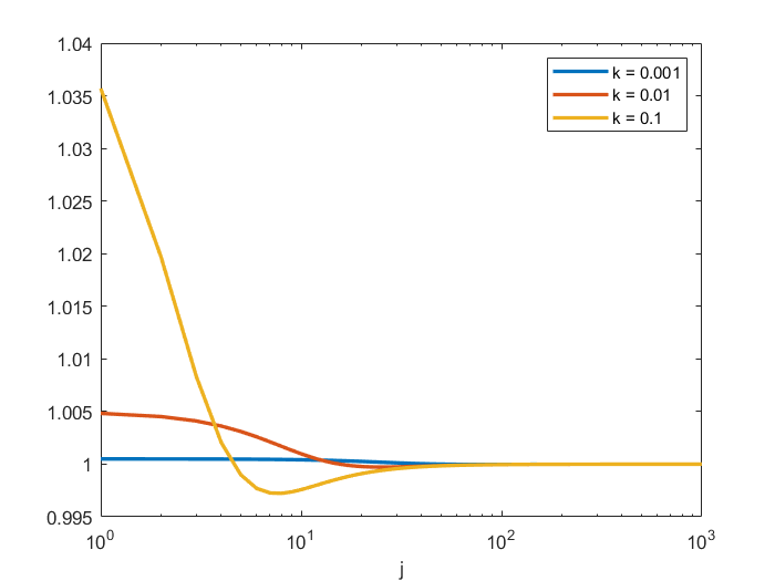
Although we do not provide associated properties of the asymptotic behavior of $V_{j}$ as $j\to\infty$ as we did for the asymptotic behavior of $f(x)$ as $x\to\infty$, we compare the behavior of $V_{j}$ with the discrete counterpart of $g(t)$, i.e. $W_{j}$, for $j=1,\ldots,100$ in Figure 2.

The main result in Section 3, i.e., Theorem 3.1 follows from Lemmas 3.1 and 3.2. In this section, we provide the proofs of both Theorem 3.1 and Lemma 3.2. For the proof of Lemma 3.1 we refer to [6].

References

• [1] E. Akin-Bohnera and J. Hoffackerb, Oscillation properties of an Emden-Fowler type equation on discrete time scales, Journal of Difference Equations and Applications 9 (2003), no. 6, 603–612.
• [2] I. Astashova, J. Diblík, and E. Korobko, Existence of a solution of discrete Emden-Fowler equation caused by continuous equation, Discrete & Continuous Dynamical Systems - S 14 (2021), no. 12, 4159.
• [3] A. Aveklouris, M. Vlasiou, and B. Zwart, A stochastic resource-sharing network for electric vehicle charging, IEEE Transactions on Control of Network Systems 6 (2019), no. 3, 1050–1061.
• [4] M.E. Baran and F.F. Wu, Network reconfiguration in distribution systems for loss reduction and load balancing, IEEE Transactions on Power Delivery 4 (1989), no. 2, 1401–1407.
• [5] R. Bellman, Stability Theory of Differential Equations, 1953.
• [6] M.H.M. Christianen, J. Cruise, A.J.E.M. Janssen, S. Shneer, M. Vlasiou, and B. Zwart, Comparison of stability regions for a line distribution network with stochastic load demands, Preprint available at: https://arxiv.org/abs/2201.06405 (2022).
• [7] H.T. Davis, Introduction to nonlinear differential and integral equations.
• [8] J. Diblík and I. Hlavičková, Asymptotic properties of solutions of the discrete analogue of the Emden-Fowler equation, Advances in Discrete Dynamical Systems, 2019, pp. 23–32.
• [9] B.A. Dubrovin, A.T. Fomenko, and S.P. Novikov, Modern Geometry - Methods and Applications, Part I:The geometry of surfaces, transformation groups, and fields, vol. 104, 1985.
• [10] L. Erbe, J. Baoguo, and A. Peterson, On the asymptotic behavior of solutions of Emden-Fowler equations on time scales, Annali di Matematica Pura ed Applicata 191 (2012), no. 2, 205–217.
• [11] R.H. Fowler, The Solutions of Emden’s and Similar Differential Equations, (1930).
• [12] W.H. Kersting, Distribution System Modeling and Analysis, fourth ed., CRC Press, 2018.
• [13] S.H. Low, Convex relaxation of optimal power flow - Part i: Formulations and equivalence, IEEE Transactions on Control of Network Systems 1 (2014), no. 1, 15–27.
• [14] B.N. Mehta and R. Aris, A note on a form of the Emden-Fowler equation, Journal of Mathematical Analysis and Applications 36 (1971), no. 3, 611–621.
• [15] J. Migda, Asymptotic properties of solutions to difference equations of emden–fowler type, Electronic Journal of Qualitative Theory of Differential Equations 2019 (2019), no. 77, 1–17.
• [16] D.K. Molzahn and I.A. Hiskens, A Survey of Relaxations and Approximations of the Power Flow Equations, A Survey of Relaxations and Approximations of the Power Flow Equations 4 (2019), no. 1, 1–221.
• [17] J.S.W. Wong, On the Generalized Emden-Fowler Equation, Society for Industrial and Applied Mathematics 17 (1975), no. 2, 339–360.