Eddy-Viscous Modeling and the Topology of Extreme
Circulation Events in Three-Dimensional Turbulence
Abstract
We discuss the role of particular velocity field configurations – instantons, for short – which are supposed to dominate the flow during the occurrence of extreme turbulent circulation events. Instanton equations, devised for the stochastic hydrodynamic setup of homogeneous and isotropic turbulence, are applied to the interpretation of direct numerical simulation results. We are able in this way to model the time evolution of extreme circulation events for a broad range of scales, through the combined use of eddy viscosity phenomenology and exact creeping instantons. While this approach works well for the core of circulation instantons, it fails to describe their tails. In order to overcome this difficulty, we put forward a numerical treatment of the axisymmetric instanton equations. Circulation instantons are then found to have a surprising topological structure, which consists of a system of paired counter-rotating vortex rings centered around the symmetry axis of a background axisymmetric vortical flow.
I Introduction
Predicting extreme events is a fundamental problem in completely distinct domains of science and technology, as in astrophysics aschwanden2019self; larrodera2021estimation, climatology bouchet2014stochastic; laurie2015computation, wind power generation couto2021identification, and a further broad list of other important contemporary fields such as finance rocco2014extreme, meteorology yiou2004extreme; grotjahn2016north and seismology soloviev2008transformation. Extreme events often take place in relatively very short time scales, but their consequences can be perennially disastrous as in the case of earthquakes, hurricanes and financial market crashes.
Navier-Stokes dynamics, our specific focus in this work, is a particularly interesting instance for the study of extreme events. The formation of intense energy-carrying localized structures in turbulent flows is a fingerprint of the non-local and nonlinear aspects of the underlying equations of motion. Fast spatial variations of the dissipation field or of the entangled system of vortex tubes which confine strong vorticity yoshida2000statistical; kaneda2003energy are, however, difficult to observe, and decades went by until it was realized that the self-similar cascade picture of turbulence, originally proposed by Kolmogorov (K41) frisch, should be revised to include the existence of such extreme events. As it is well known, the predicted K41 scaling exponents for the statistical moments of velocity differences fail to reproduce the respective numerically and experimentally measured values batchelor1949nature; anselmet1984high; vincent1991spatial at high moment orders. Commonly understood as an important feature of the intermittency phenomenon frisch; kaneda2003energy, these deviations of the K41 scaling exponents have been accurately obtained through multifractal formulations kolmogorov1962refinement; obukhov1962; novikov1994intermittency; she1994universal; apolinario2020vortex; pereira2022hard, but more fundamental derivations are still in order.
A systematic analytical strategy to address the problem of intermittent velocity fluctuations was initially introduced in the framework of Burgers turbulence burgers1948mathematical. Asymptotic results were found for the right tail of the velocity gradient probability distribution functions gurarie1996instantons, based on the steepest-descent approximation as implemented in the Martin-Siggia-Rose-Janssen-de-Dominicis martin1973statistical; janssen1976lagrangean; dominicis1976technics (MSRJD) functional formalism. Subsequent theoretical and numerical efforts have been made to describe the left tail of Burgers velocity gradient and velocity difference PDFs balkovsky1997intermittency; chernykh2001large; moriconi2009instanton; grafke2015relevance; apolinario2019onset. Despite the relevant progress achieved for the Burgers and effective Lagragian turbulent models johnson2016closure; grigorio2017instantons; apolinario2019instantons; alqahtani2021extreme, the description of intermittency in three-dimensional turbulence is still very open to investigation along the lines of the MSRJD approach.
In this work, we use the MSRJD functional formalism to study the scaling properties of velocity circulation in three-dimensional homogeneous and isotropic turbulence, motivated by the fact that velocity circulation fluctuations are known to provide clear signatures of turbulence intermittency umeki1993probability; migdal1994loop; cao1996properties; benzi1997self. Velocity circulation is a natural tool to probe localized vortex structures, which contain most of the turbulent kinetic energy in high Reynolds number flows kaneda2003energy; frisch. The first formally structured attempt to explore velocity circulation as the main actor of turbulent fluctuations dates back to 1994 migdal1994loop. Promising results about the circulation probability distribution functions (cPDFs) were then advanced, but further developments and validation studies faced serious obstacles in the following years, due to computational limitations. More recently, once hardware shortcomings were overcome, the subject of circulation statistics was vigorously revisited under the light of much improved high-resolution simulations, not only in classical iyer2019circulation; iyer2021area but also in quantum turbulence muller2021intermittency; polanco2021vortex. Interesting perspectives on the multifractal and structural views of classical turbulence cascades have been put forward since then apolinario2020vortex; pereira2022hard; moriconi2021multifractality; moriconi2022statistics.
Throughout our considerations, the circulation variable is defined as
| (1) |
where is a circular domain of radius and is the circular contour that encloses . The fields and are, respectively, the velocity and vorticity fields related through (we use Einstein notation for the summation over repeated indices, unless explicitly stated). We are interested in discussing velocity field configurations – instantons, for short – which are associated to extreme circulation events, that is, large deviations of . On one front of analysis, we model them as exact creeping flow structures creeping related to turbulent eddy-viscosity boussinesq1877essai time scales. The approach proves to be phenomenologically meaningful, once we validate it by means of extensive turbulence databases. On another front, we numerically solve the axisymmetric nonlinear instanton equations, to find that the circulation instantons have a remarkable topological structure described by the superposition of two counter-rotating vortex rings that share the same symmetry axis and carry opposite helicity in the presence of a background axial vorticity field.
This paper is organized as follows. Sec. II briefly reviews the main technical aspects of the MSRJD functional formalism. We, then, obtain closed analytical solutions for the circulation instantons in the viscous limit of the Navier-Stokes equations and show their somewhat unexpected usefulness to model the time evolution of extreme circulation events, from the analysis of direct numerical simulation (DNS) data. The nonlinear instanton equations are introduced in Sec. III, and their numerical solutions are carefully discussed, with emphasis placed on the qualitative differences between them and the creeping solutions derived in Sec. II. Finally, in Sec. IV, we summarize our findings and indicate directions of further research.
II The functional approach and creeping instantons
II.1 MSRJD Formalism
Many physical systems which exhibit extreme events among their dynamical states are suitable for the application of large deviation techniques weiss1995introduction; evertsz1995large; ragone2018computation. It is often possible to address in these cases the MSRJD methodology martin1973statistical; janssen1976lagrangean; dominicis1976technics, where one typically deals with differential equations that lead to solutions – the so-called instantons – which dominate the probability distribution tails that describe the occurrence of extreme events.
We are interested in applying these ideas to three-dimensional turbulence in its stochastic hydrodynamics formulation brenig1976stochastic. The stochastic incompressible Navier-Stokes equations are written as
| (2) |
| (3) |
where is the velocity field, is the pressure field ensuring the incompressibility constraint (Eq. 3), is the kinematic viscosity, and is a zero-average Gaussian random field used to model large-scale forcing, correlated as
| (4) |
The exact form of is not phenomenologically relevant insofar as its correlation length is much larger than the investigated length scales. Assuming homogeneity and isotropy, the correlation kernel depends only on and is parametrized by its amplitude and its correlation length , which can be conveniently defined as .
In our particular application of the MSRJD formalism, we deal with a functional measure which is path-integrated over and an auxiliary field ivashkevich1997symmetries; grafke2015instanton. Lagrange multipliers and are also introduced, to ensure incompressibility and to fix the circulation at a given time instant, respectively. More concretely, the cPDF is evaluated in the MSRJD formalism as
| (5) |
where the pseudo-statistical weight (it is a complex number) contributions for are given as the exponential of the MSRJD action, , specified below, and is an unimportant normalization constant (to be suppressed hereafter). A single dimensionless parameter can be factored out from the action and its role is to control the noise strength and to set what should be considered an extreme event: these are the ones associated to MSRJD actions which are much larger than .
The above functional integration represents the probability density functional to find velocity circulation as defined in Eq. (1), at a particular time instant, namely , due to the cumulative effect of forcing since the remote past, say . All fields are assumed to vanish in the remote past. Moreover, instantons are restricted to , such that auxiliary fields are imposed to vanish at as a boundary condition chernykh2001large. Measuring length in units of and time in units of the viscous time scale
| (6) |
a dimensionless form of the MSRJD action can be written as
| (7) |
where, now, is the force-force correlator with unit correlation length. The connection between and the Reynolds number Re is made by the assumption that a well defined inertial range develops when the dissipation length is much smaller than the correlation length . Since the characteristic velocity scale is , we obtain, as a consequence, that Re .
Instantons correspond to the extrema of the MSRJD action and are assumed to provide, from Eq. (II.1), the dominant saddle-point contributions in the path-integral evaluation of extreme event probabilities. They are found as solutions of the variational principle , which amounts here to the instanton equations,
| (8) |
| (9) |
subject to the constraints,
| (10) |
| (11) |
By solving the above equations, one gets asymptotic expressions for the cPDF tails, from the mapping of the values of the Lagrange multiplier to the final velocity circulation . The instanton calculus yields, in this way,
| (12) |
as an asymptotic approximation that holds for , where and is a normalization constant. A more mathematically rigorous discussion of the arguments leading to results which are analogous to (12) is the essential subject of large deviation theory dembo1998large. As a direct consequence of the Gärtner-Ellis theorem, a probability density function necessarily follows the Large Deviation Principe (Eq. (12), in our case) if the associated action is strictly convex and the map between and the observable of interest is differentiable for an arbitrary . Non-convex actions or ill-defined -maps can be nevertheless adapted to large deviation evaluations through the use of alternative integration measures alqahtani2021instantons.
II.2 Creeping Instantons and Eddy Viscous Modeling
Instanton equations are rarely amenable to analytical treatment without the help of phenomenological or empirical inputs about the underlying dynamics. Approximate solutions of (8-11) and of analogous magnetohydrodynamic equations were formerly carried out under restrictive assumptions about the roles of symmetries and the strain rate field moriconi1998circulation; moriconi2002circulation. Somewhat surprisingly, as we will discuss in the following, interesting information on extreme events can be obtained from the exact form of viscous (creeping) instantons.
To work out the creeping instantons, we introduce the diffusion Green’s function with vanishing boundary condition in ,
| (13) |
Neglecting the nonlinear terms in Eqs. (8-11), the velocity and the conjugate solutions read
| (14) |
| (15) |
The MSRJD action, Eq. (II.1), additionally reduces to
| (16) |
Defining, at this point, the explicit form of the force-force correlator as
| (17) |
we obtain from (14) and (15) the creeping instanton solution by setting to be perpendicular to the contour
| (18) |
where is the modified Bessel function of the first kind and . We remark that part of the spatio-temporal dependence of the velocity field is encoded in the upper limit of the above integration. It is interesting to note that this integral can be exactly computed only at points that belong to the contour , defined by and . We find, in cylindrical coordinates,
| (19) |
where is the hypergeometric function of entries. The time-dependent instanton circulation is readily obtained as
| (20) |
Since the circulation is a linear function of , the resulting cPDF is Gaussian. Recovering the original circulation units, its variance is found to satisfy
| (21) |
We have, for ,
| (22) |
such that, in this asymptotic limit,
| (23) |
Although (23) is expected to hold only for creeping flows, it may be possibily relevant even for higher Reynolds number solutions, once scales are probed and the MSRJD path-integration (II.1) is dominated by smooth velocity field configurations. The educated guess that generalizes (23) to turbulent flows sustained by alternative forcing mechanisms, where and Re are not necessarily defined in terms of Gaussian force-force correlators, reads
| (24) |
To investigate the correctness of (24), we have worked with four DNS datasets of homogeneous and isotropic turbulent flows, publicly available from the Johns Hopkins Turbulence Database (JHTDB) platform11 1 For more information about the public datasets see http://turbulence.pha.jhu.edu/. perlman2007data; JHTD2; JHTD3; JHTD4. The simulations were developed in periodic cubic lattices with dimensions (dataset I), (datasets II), and (datasets III and IV), corresponding to Taylor-based Reynolds numbers 418, 610, 613 and 1280 for datasets from I to IV. We have produced from these datasets ensembles which contain respectively , , , and circulation samples, computed by employing the first equality of Eq. (1). Denoting by the Kolmogorov dissipation length frisch, the results reported in Fig. 1 fully corroborate our expectations: relation (24) is in fact verified for (it should be noted that small scale evaluations of are subject to relatively larger error bars, due to the inaccuracy associated to the representation of a circular contour in a square lattice, as closed polygonal line).
Fig. 1 also shows that the LHS of (24) leads, incidentally, to an excellent collapse of data across the inertial range scales . Furthermore, the circulation variance has, in this range, a scaling dependence with which is very well approximated by the K41 scaling exponent iyer2019circulation, as indicated by a dashed line Note that at fixed integral scale and fixed energy injection rate per unit mass, , relation (24) implies that . Insisting that an analogous result should hold in the inertial range, we replace in this last relation by the scale-dependent eddy viscosity smith1998renormalization,
| (25) |
where and are some reference viscosity and length scale parameters, to obtain the observed scaling .
As a brief historical digression, we point out that the concept of eddy viscosity, long ago conceived by Boussinesq boussinesq1877essai and much later revived through the distant interaction approximation (DIA) formalism kraichnan1964decay and dynamical renormalization group techniques forster1977large; yakhot1986renormalization, is essentially an effective transport parameter that allows for a coarse-grained description of the turbulent cascade. This is the main physical motivation for a number of numerically tractable models of turbulence, as the celebrated Smagorinsky sub-grid formulation of the Navier-Stokes equations smagorinsky1963general; scotti1993generalized, which underlies the whole field of large eddy simulations germano1991dynamic; mason1994large; piomelli1999large; piomelli2014large.

The replacement of the molecular viscosity by the eddy viscosity in (24) sounds at this point like a purely rhetoric remark. It is possible, however, that creeping instantons, when combined with eddy viscosity ideas, can in fact be used to model the time evolution of high Reynolds number circulation instantons. The argument goes as follows. Consider the set of all flow realizations which have evolved from the remote past and ended with extreme circulation
| (26) |
at time , where ( is just a measurement bin). Let now represent the time averaged circulation taken over the ensemble of all of these flow realizations, which we refer to as the filtered instanton circulation. Resorting to dynamic similarity and to the fact that (i.e., Reynolds number is high), we write down the dimensionless circulation ratio (time units are restored to the original ones, from now on),
| (27) |
It follows from Eq. (27) that
| (28) |
In consonance with eddy viscosity phenomenology, we assume that Eq. (28) is scale invariant, viz.,
| (29) |
We note that Eq. (29) is just a renormalization group equation smith1998renormalization, which has, as general solution, the functional relationship
| (30) |
This leads us, from (27), to
| (31) |
with
| (32) |
where we have used (25) to make the -dependence explicit in the definition of .
In an analogous fashion, one has for the exact viscous solution (20)
| (33) |
It is natural to conjecture, furthermore, that in the limit , the filtered and the viscous instanton circulations match, that is,
| (34) |
Pushing the validity of Eq. (30) down to dissipative scales, we get
| (35) |
which, in view of (34), leads to
| (36) |
Comparing (36) with (30), it follows that
| (37) |
so that can be modeled, from (31), as the viscous instanton solution , that is,
| (38) |
In order to perform validation tests of Eqs. (31) and (38), we have implemented a numerical filtering procedure to extract, from the raw data of the JHTDB, the past time evolutions of extreme circulation events, which we detail below.
II.3 Numerically Filtered Circulation Instantons
We have taken Dataset I for statistical analyses, since this is the dataset which allows us to work with the largest ensemble of circulation time series, defined for circular contours centered at equally spaced grid points. Letting be the lattice parameter (), we have studied circulation fluctuations for four different radii, namely, , , , and . For each given radius, we considered circular contours oriented normally to each Cartesian direction, for a total of contours per radius.
We conventionally define the set of extreme events as the ensemble of circulations events whose absolute values reach some multiple of the circulation standard deviation, , within a small tolerance window. In the language of Eq. (26), we consider the interval defined by with a 0,5% tolerance, that is, .

Once an extreme circulation event belonging to a given set is identified, we assign it the observation time instant and save its earlier time evolution. Then, a time dependent average over all saved series for each set is computed. Similar filtering procedures have been applied in instanton studies of Burgers turbulence grafke2013instanton, Lagrangian turbulence models grigorio2017instantons; apolinario2019instantons and rogue wave formation dematteis2018rogue; dematteis2019experimental.
Our results for are shown in Fig. 2. Taking as an arbitrary reference length scale, we find that plots of as a function collapse reasonably well for all the investigated radii and sets , as predicted by (31). Following now Eq. (38), we carry out an -norm minimization of
| (39) |
to adjust as the reference viscosity in (25). Meaningful comparisons are then also reported in the same Fig. 2 for the eddy viscous modeling of , as suggested by (32) and (38).

In addition to the eddy viscous modeling of the filtered circulations discussed above, one may wonder whether the functional forms of filtered instanton velocity fields could be effectively modeled by viscous instantons as well. With this aim, we take the symmetry axis of each prescribed circular contour as the -axis of a local Cartesian reference system, and orient it in such a way that velocity circulations are rendered positive at the event occurrence time. Then, we perform a similar time-dependent averaging procedure over all events in , as we did for , but now for velocity field configurations in cylindrical coordinates, . Due to isotropy, the mean velocity components are functions of , , and only, i.e., , , and .
Unfortunately, the radial and axial components and turn out to develop relatively small intensities, which prevents us from extracting a clear behavior out of the noise. The mean azimuthal component , on the other hand, was found to be well-resolved in all studied cases. Fig. 3 shows comparisons between the numerically filtered (normalized by ) and the analogous normalized azimuthal velocity obtained from the viscous solution (18), where the dimensionless time is substituted by , as defined in Eq. (32). It is seen that the eddy viscous modeling only provides an adequate description of for , which is just the core region of the filtered instantons. Notwithstanding such a limitation, extreme circulations events are in fact well accounted by eddy viscous modeling, since, as the filtering results indicate, gets its maximum value at .
III nonlinear Instantons
A numerical scheme to solve the hydrodynamic instanton equations, similar to Eqs. (8-9), was introduced by Chernykh and Stepanov chernykh2001large in the context of Burgers turbulence, being later extended to a variety of models dematteis2018rogue; dematteis2019experimental. In our case, the solution algorithm inserts, at “iteration step ”, a given velocity field in Eq. (9) to solve it backward in time. Its solution is defined as the auxiliary field at iteration step . This, in turn, is used in Eq. (8) to provide the velocity field at iteration step . An iteration cycle proceed recursively, until a prescribed convergence for the instanton fields is attained. The numerical procedure may start off with a vanishing velocity field or one may alternatively use some improved guess, as we do by using the creeping instanton described by (18).
We have worked out solutions for the circulation instantons in cylindrical coordinates with Chebyshev collocation points (see the appendix for details) for a broad range of values and contour radii. The numerical solutions were obtained through the Chernykh-Stepanov method outlined above, enhanced, at larger values of , by the convexification procedure discussed in alqahtani2021instantons, in order to avoid possible spoiling inflection effects in the derivation of the cPDF tails. This amounts, in practical terms, to perform the replacement of by the nonlinear tilted measure in the MSRJD action (II.1).

Instability issues are known to affect the convergence of the Chernykh-Stepanov solutions at large values of the Lagrange multiplier alqahtani2021instantons. Although a number of technical improvements have been implemented to solve instanton equations in more efficient ways grafke2014arclength; grafke2019numerical; grigorio2020parametric, three-dimensional instanton equations are far more computationally expensive than their dimensionally reduced counterparts.
Fig. 4 yields the typical velocity profile of a circulation instanton. A threefold vortex structure emerges, with interesting topological properties. It consists of two paired counter-rotating vortex rings, as they can be clearly identified from the streamline portrait there depicted in the plane. These rings define regions of opposite helicities, a fact associated to the background axisymmetric velocity field that circulates around the symmetry axis of the flow.
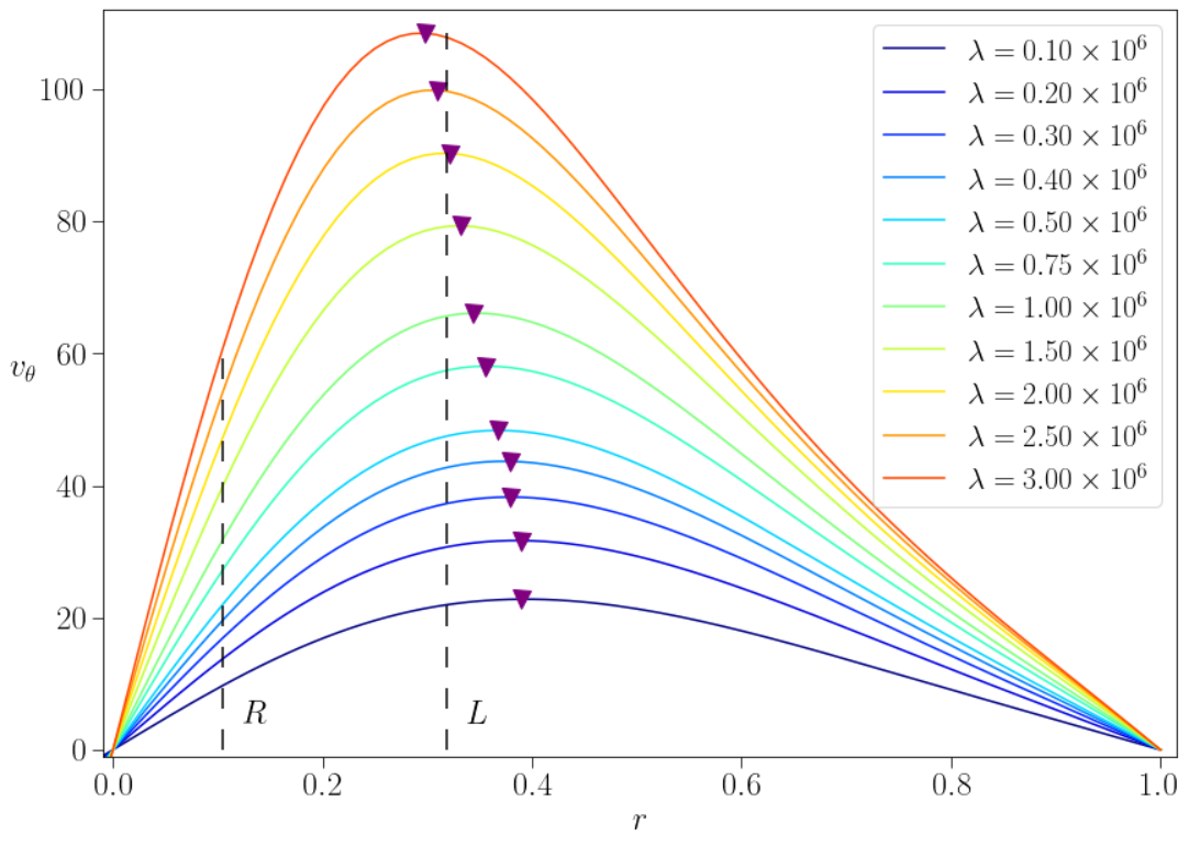
It is not difficult to see, from Fig. 4, that the azimuthal component of the velocity field is not peaked at as we have found in our analysis of the filtered DNS instantons (extreme circulation events), previously summarized in Fig. 3. This is not a completely casual remark. In fact, it turns out that the coupled instanton equations (8-11) become very stiff at large values of , precisely where we expect to model asymptotically large circulation fluctuations.
In Fig. 5 we show that, as grows, the peak position of slowly drifts to the left (smaller values of ). A rough estimate indicates that a peak at would be reached for , which is several orders of magnitude beyond the domain of convergence achieved in our applications of the Chernykh-Stepanov method.
We find, thus, that direct numerical schemes to solve the instanton equations (8-11), like the ones we have applied, are able to address the parabolic cores of cPDFs, while the description of their tails remains challenging. In order to circumvent the stiffness of the instanton equations, and to model the far cPDF tails, space-time reparametrizations chernykh2001large; grafke2014arclength; grigorio2020parametric and further large deviation techniques are likely to be necessary, as illustrated by the use of hybrid Monte Carlo algorithms, so far only applied to Burgers turbulence margazoglou2019hybrid.
IV Conclusions
We have investigated the occurrence of extreme circulation events in three-dimensional homogeneous and isotropic turbulence. We show that the time evolution of circulation, conditionally averaged to the observation of prescribed large deviation events can be effectively modeled with the help of eddy-viscosity phenomenology combined with instanton functional techniques. Our modeling analysis is corroborated from a careful treatment of large DNS databases, at various Reynolds numbers.
Proceeding with the same set of extreme circulation events, we have furthermore inspected time-dependent conditionally averaged velocity field configurations. Resulting axisymmetric vortex structures clearly arise from these filtering procedures. The comparison with the eddy-viscous (creeping) instantons is only reasonable at the core of the flow configurations (circulation instantons), which, nevertheless, is all one needs to get accurate averages of the time-dependent instanton circulations ending in extreme events.
An extensive numerical effort to solve the instanton equations suggests that extreme circulation events have an interesting underlying topological structure. Axisymmetric circulation instantons are composed of a main vortex, which is at the center of a surrounding pair of counter-rotating vortex rings. The existence of this triple vortex structure drives our attention to possible formal connections with superfluidity. It is known that the motion of a superfluid vortex ring is followed by a companion pair of normal vortex rings kivotides2000triple. We note, then, that the instanton Eqs. (8) and (9) are actually analogous to the HVBK hydrodynamic equations describing the self-induced propagation of a quantum vortex ring.
Although the employed numerical databases allowed us to validate a viscous-eddy modeling of extreme circulation events, they are not large enough to disclose the topological features of the circulation instantons. Larger databases are required, in order to accomplish this challenging task. Another related important issue, deserved for further studies, has to do with the implementation of algorithmic improvements in the numerical solution of the instanton equations, in order to model the far cPDF tails iyer2019circulation; iyer2021area and the off-core azimuthal velocity component of the circulation instantons. It is worth emphasizing that some alternatives have been already applied with success to the paradigmatic example of Burgers turbulence grafke2014arclength; grafke2015relevance.
Intense vortex structure is known to have an important role in turbulence at high Reynolds numbers. Such structures can be modeled by an interacting molecular gas when statistical properties of circulation in 2D slices of turbulent flows are analyzed apolinario2020vortex; moriconi2021multifractality; moriconi2022statistics; pereira2022hard. A possible source of future investigation is to explore a single or a bunch of modeled structures in order to compare its spatial distribution to the instanton solutions.
Acknowledgement
This work has been partially supported by CAPES via Grant No. 88887.336246/2019-00 (V.J.V.) and by the Simons Foundation Award ID 651475 (G.B.A.).
References
- (1) M.J. Aschwanden, ApJ 880, 105 (2019).
- (2) C. Larrodera, L. Nikitina, and C. Cid, Space Weather 19, e2021SW002902 (2021).
- (3) F. Bouchet, C. Nardini, and T. Tangarife , Fluid Dyn. Res. 46, 061416 (2014).
- (4) J. Laurie and F. Bouchet, New. J. Phys. 17, 015009 (2015).
- (5) A. Couto, P. Costa, and T. Simões, Energies 14, 3944 (2021).
- (6) M. Rocco, J. Econ. Surv. 28, 82 (2014).
- (7) P. Yiou and M. Nogaj, Geophys. Res. Lett. 31, (2004).
- (8) R. Grotjahn, R. Black, R. Leung, M.F. Wehner, M. Barlow, M. Bosilovich, A. Gershunov, W.J. Gutowski, J.R. Gyakum, R.W. Katz, et al, Clim. Dyn. 46, 1151 (2016).
- (9) A. Soloviev, Nonlinear Process Geophys 15, 209 (2008).
- (10) K. Yoshida and N. Hatekeyama, J. Phys. Soc. Japan 69, 1661 (2000).
- (11) Y. Kaneda, T. Ishihara, M. Yokokawa, K. Itakura, and A. Uno, Phys. Fluids 15, L21 (2003).
- (12) U. Frisch, Turbulence, (New York, Cambridge University Press, 1995).
- (13) G.K. Batchelor and A.A. Townsend, Proc. R. Soc. A: Math. Phys. Sci. 199, 238 (1949).
- (14) F. Anselmet, Y. Gagne, E.J. Hopfinger, and R.A. Antonia, J. Fluid Mech. 140, 63 (1984).
- (15) A. Vincent and M. Meneguzzi, J. Fluid Mech. 225, 1 (1991).
- (16) A.M. Obukhov, J. Fluid Mech. 13, 77 (1962).
- (17) A.N. Kolmogorov, J. Fluid Mech. 13, 82 (1962).
- (18) E. Novikov and R. Stewart, Izv. Geophys. Ser 3, 408 (1964).
- (19) Z.S. She and E. Leveque, Phys. Rev. Lett. 72, 336 (1994).
- (20) G.B. Apolinário, L. Moriconi, R.M. Pereira and V.J. Valadão, Phys. Rev. E 102, 041102 (2020).
- (21) L. Moriconi, R.M. Pereira, and V.J. Valadão, arXiv:2205.10470.
- (22) J.M. Burgers, Adv. Appl. Mech. 1, 171 (1948).
- (23) V. Gurarie and A. Migdal, Phys. Rev. E 54, 4908 (1996).
- (24) P.C. Martin, E.D. Siggia, and H.A. Rose, Phys. Rev. A 8, 423 (1973).
- (25) H.K. Janssen, Z. Phys. B: Cond. Mat. 23, 377 (1976).
- (26) C. de Dominicis, J. Phys. Colloque 37, C1–247 (1976).
- (27) E. Balkovsky, G. Falkovich, I. Kolokolov, and V. Lebedev, Phys. Rev. Lett. 78, 1452 (1997).
- (28) A.I. Chernykh and M.G. Stepanov, Phys. Rev. E 64, 263061 (2001).
- (29) L. Moriconi, Phys. Rev. E 79, 046324 (2009).
- (30) T. Grafke, R. Grauer, T. Schäfer, and E. Vanden-Eijnden, Eur. Phys. Lett. 109, 34003 (2015).
- (31) G.B. Apolinário, L. Moriconi, and R.M. Pereira, Phys. Rev. E 99, 033104 (2019).
- (32) P.L. Johnson and C. Meneveau, J. Fluid Mech. 804, 387 (2016).
- (33) L.S. Grigorio, F. Bouchet, R.M. Pereira, and L. Chevillard, J. Phys. A: Math. Theor. 50, 055501 (2017).
- (34) G.B. Apolinário, L. Moriconi, and R.M. Pereira, Phys. A: Stat. Mech. Appl. 514, 741 (2019).
- (35) M. Alqahtani, L. Grigorio, and T. Grafke, arXiv:2108.02103.
- (36) M. Umeki, J. Phys. Soc. Japan 62, 3788 (1993).
- (37) A. Migdal, Int J Mod Phys A 9, 1197 (1994).
- (38) N. Cao, S. Chen, and K.R. Sreenivasan, Phys. Rev. Lett. 76, 616 (1996).
- (39) R. Benzi, L. Biferale, M.V. Struglia, and R. Tripiccione, Phys. Rev. E 55, 3739 (1997).
- (40) K.P. Iyer, K.R. Sreenivasan, and P.K. Yeung, Phys. Rev. X 9, 041006 (2019).
- (41) K.P. Iyer, S.S. Bharadwaj, and K.R. Sreenivasan, Proc. Natl. Acad. Sci. U.S.A. 118, e2114679118 (2021).
- (42) N.P. Müller, J.I. Polanco, and G. Krstulovic, Phys. Rev. X 11, 011053 (2021).
- (43) J.I. Polanco, N.P. Müller, and G. Krstulovic, Nat. Commun. 12, 7090 (2021).
- (44) L. Moriconi, Phys. Rev. E 103, 062137 (2021).
- (45) L. Moriconi and R.M. Pereira, arXiv:2204.12862.
- (46) P.A. Durbin and G. Medic, Fluid Dynamics with a Computational Perspective, (Cambridge, Cambridge University Press, 2010).
- (47) J. Boussinesq, Mem. Pres. Par Diu. Sav. Acad. Sci. Paris 23, 46 (1877).
- (48) A. Weiss, IEEE JSAC 13, 938 (1995).
- (49) C. Evertsz and K. Berkner, Chaos Solit. Fractals 6, 121 (1995).
- (50) F. Ragone, J. Wouters, and F. Bouchet, Proc. Natl. Acad. Sci. U.S.A. 115, 24 (2018).
- (51) L. Brenig, M. Malek-Monsour, and W. Horsthemke, Phys. Lett. A 59, 341 (1976).
- (52) E. Ivashkevich, J. Phys. A: Math. Gen. 30, L525 (1997).
- (53) T. Grafke, R. Grauer, and T. Schäfer, J. Phys. A: Math. Theor. 48, 333001 (2015).
- (54) A. Dembo and A.D.O Zeitouni, Large deviations techniques and applications, (Berlin, Springer, 2010).
- (55) M. Alqahtani and T. Grafke, J. Phys. A: Math. Theor. 54, 175001 (2021).
- (56) L. Moriconi and F. Takakura, Phys. Rev. E 58, 3187 (1998).
- (57) L. Moriconi and F. Nobre, Phys. Rev. E 65, 036302 (2002).
- (58) E. Perlman, R. Burns, Y. Li, and C. Meneveau, Proc. ACM/IEEE, 1 (2007).
- (59) P.K. Yeung, D.A. Donzis, and K.R. Sreenivasan, J. Fluid Mech. 700, 5 (2012).
- (60) P.K. Yeung, X.M. Zhai, and K.R. Sreenivasan, Proc. Natl. Acad. Sci. U.S.A. 112, 12633-12638 (2015).
- (61) P.K. Yeung, K.R. Sreenivasan, and S.B. Pope, Phys. Rev. Fluids 3, 064603 (2018).
- (62) L.M. Smith and S.L. Woodruff, Annu. Rev. Fluid Mech. 30, 275 (1998).
- (63) R.H. Kraichnan, Phys. Fluids 7, 1030 (1964).
- (64) D. Forster, D.R. Nelson, and M.J. Stephen, Phys. Rev. A 16, 732 (1977).
- (65) V. Yakhot and S.A. Orszag, J. Sci. Comput. 1, 3 (1986).
- (66) J. Smagorinsky, Mon. Weather Rev. 91, 99 (1963).
- (67) A. Scotti, C. Meneveau, and D.K. Lilly, Phys. Fluids A: Fluid Dyn. 5, 2306 (1993).
- (68) M. Germano, U. Piomelli, P. Moin, and W.H. Cabot, Phys. Fluids A: Fluid Dyn. 3, 1760 (1991).
- (69) P.J. Mason, Q. J. R. Meteorol. Soc. 120, 1 (1994).
- (70) U. Piomelli, Prog. Aerosp. Sci. 35, 335 (1999).
- (71) U. Piomelli, Philos. Trans., Math. Phys. Eng. Sci. 372, 20130320 (2014).
- (72) T. Grafke, R. Grauer, and T. Schäfer, J. Phys. A: Math. Theor. 46, 062002 (2013).
- (73) G. Dematteis, T. Grafke,and E. Vanden-Eijnden, Proc. Natl. Acad. Sci. U.S.A. 115, 855 (2018).
- (74) G. Dematteis, T. Grafke, M. Onorato, and E. Vanden-Eijnden, Phys. Rev. X 9, 041057 (2019).
- (75) T. Grafke, R. Grauer, T. Schäfer, and E. Vanden-Eijnden, Multiscale Model. Simul. 12, 566 (2014).
- (76) T. Grafke and E. Vanden-Eijnden, Chaos 29, 063118 (2019).
- (77) L. Grigorio, J. Phys. A: Math. Theor. 53, 445001 (2020).
- (78) G. Margazoglou, L. Biferale, R. Grauer, K. Jansen, D. Mesterházy, T. Rosenow, and R. Tripiccione, Phys. Rev. E 99, 053303 (2019).
- (79) D. Kivotides, C.F. Barenghi, and D.C. Samuels, Science 290, 777 (2000).
- (80) C. Canuto, M. Hussaini, A. Quarteroni, and T. Zang, Spectral methods in fluid dynamics, (Berlin, Springer, 1988).
- (81) R. Peyret, Spectral methods for incompressible viscous flow, (Berlin, Springer, 2013).
- (82) K.J. Arrow, L. Hurwicz and, H. Uzawa, Studies in linear and nonlinear programming, (California, Stanford University Press, 1958).
- (83) I. Raspo, S. Hugues, E. Serre, A. Randriamampianina, and P. Bontoux, Comput. Fluids 31, 745 (2002).
- (84) J. Lopez and J. Shen, J. Comput. Phys. 139, 308 (1998).
- (85) N. Peres, S. Poncet, and E. Serre, J. Comput. Phys. 231, 6290 (2012).
- (86) T. Schorlepp, T. Grafke, S. May, and R. Grauer, arXiv:2107.06153.
*
Appendix A Spectral Approach to the Instanton Equations in Cylindrical Coordinates
In order to numerically solve the set of Eqs. (8-11) we rewrite them in cylindrical coordinates. In light of the nonlinear nature of hydrodynamic interactions, there would be no a priori reason to consider axisymmetric solutions in detriment of any other. Nevertheless, we expect axisymmetric solutions to dominate extreme events since the forcing term is invariant under rotations around the -axis. Taking this symmetry into account, Eqs. (8-11) read
| (40) |
where and is the spatial convolution between and . We implement a pseudo-spectral approach where the fields are expanded in a truncated Fourier-Chebyshev series of orders and , respectively. The collocation points are defined as
| (41) |
and
| (42) |
where, and are integers in the ranges and . Along the longitudinal direction, usual collocation points for Fourier series are used, while for the radial direction we employ Gauss-Lobatto collocation points, corresponding to the extrema of the order Chebyshev polynomials canuto1988spectral. This choice of a non-homogeneous grid hinders a direct comparison among simulations with different resolutions. However, it allows one to adopt a Fast Fourier Transform (FFT) algorithm to compute nonlinear terms, which are otherwise computationally expensive peyret2013spectral. Moreover, for even the coordinate singularity at is explicitly avoided on the collocation, with the drawback of requiring the radial inverval to be duplicated, as , as a requirement of the Chebyshev polynomial expansion.
All fieds in Eq. (40) are given by a truncated polynomial series of order in the Fourier basis and in the Chebyshev basis,
| (43) |
where is the Chebyshev polynomial. Exceptions are the pressure fields and , which are of order in the Chebyshev expansion. This guarantees the stability of the numerical method, an approach known as the approximation peyret2013spectral, further discussed ahead. Radial derivatives of these fields are readily computed using recursion relations of the Chebyshev polynomials, namely,
| (44) |
where the matrix has, for all fields but the pressure related ones, the entries
| (45) |
with and otherwise. As for the pressure fields, which are 2 degrees lower in the Chebyshev expansion, they must be interpolated from the Gauss-Lobatto grid to the grid where the other fields are defined. This can be done through a Lagrange interpolation (see Ref. peyret2013spectral for details), giving
| (46) |
By virtue of the explicit form of these matrices, -derivatives are evaluated in physical space while -derivatives are better performed in Fourier space. Ultimately, in order to have consistently represent all fields in the mirrored radial domain, they must satisfy the following reflection properties:
| (47) |
The time discretization follows a combined Adams-Bashforth/Implicit Backward Differentiation method of second order (AB/BDI2) peyret2013spectral, which consists on implicit evaluations of the linear terms and explicit evaluations of the nonlinear terms. As an illustration, consider the equation
| (48) |
where, and stand for the linear and nonlinear terms of the differential equation, respectively, and accounts for a forcing term or pressure gradient. The above equation is discretized at regularly spaced time instants as
| (49) |
where . In the first time step, we set and change , reducing this step to the usual Euler scheme. The choice of discretizing the pressure gradient terms as leads to a Stokes problem which is solvable by the Uzawa method uzawa1958iterative. We note that similar discretization setups were successfully applied to the Navier-Stokes equations in cylindrical coordinates with a few different boundary conditions raspo2002spectral; lopez1998efficient; peres20123d. We also remark that the nonlinear terms are properly de-aliased following a standard 3/2-rule.
Applying the above discretization procedure to the system of Eqs. (40) supplemented by Dirichlet boundary conditions, one finds a system of coupled equations for each independent Fourier mode for the forward and backward time integration of the velocity and conjugate field, respectively,
| (50) |
where the ket notation represents the -dimensional vector with . The matrices , and can be efficiently inverted and stored in a pre-processing stage. The vectors and are, respectively, the explicit part of the discretized Eqs. 8 and 9. For instance, in Eq. 49 one has .
The algebraic system defined by Eq. 50 has a unique solution for every . The approximation prevents zero eigenvalues of the Uzawa operator22 2 The Uzawa operator is obtained by solving formally the pressure field by setting the momentum equations into the incompressibility constraint, in this case . for and avoids the requirement of prescribing boundary conditions to the pressure field. Indeed, non-uniqueness of the solution is related to the fact that pressure fields are defined up to a constant and a simple calculation shows that the unique solution consistent with the boundary conditions and the incompressibility constraint for is .
The convolutions in Eq. (40) and in the action integral (Eq. II.1) can be efficiently computed using the explicit form of the Fourier transformed correlation and the inverted Chebyshev derivative matrix,
| (51) |
| (52) |
where , , for , and for , with being modified Bessel functions of the first kind.
In order to validate the numerical method, we performed several numerical experiments of the linear instanton. Fig. 6 compares the component of the numerical solution with the analytical result from Eq. 18. We first note that the Dirichlet boundary condition has a relevant influence on the solution for . This is not a surprising though, since Eq. 18 holds for unbounded domains, thus a slower decay is expected. Variations of about in the peak position are also observed depending on how distant to the boundaries one sets and . We fixed to minimize such boundary effects.

The viscous action was calculated by means of Eq. 52, and it was found to be compatible with with and , with errors estimated by averaging results obtained with different grid resolutions, both in time and space. Small variations of are seen when and/or are changed, but one must keep in mind that the radial collocation is not regular, and hence direct comparisons among different resolutions in are not perfect. As for the dependence, finite time effects are in play, since decreasing for a fixed number of timesteps also causes the total simulation time to decrease, so the boundary conditions are effectively imposed on different time instants . In out tests, we worked with all combinations of , , and , with , , and .
The conclusion drawn from this set of numerical experiments is that both spatial and statistical properties are accurately captured by the numerical algorithm used to solve the instanton equations, at least in the linear approximation.