Automatic Depth Optimization for Quantum Approximate Optimization Algorithm
Abstract
Quantum Approximate Optimization Algorithm (QAOA) is a hybrid algorithm whose control parameters are classically optimized. In addition to the variational parameters, the right choice of hyperparameter is crucial for improving the performance of any optimization model. Control depth, or the number of variational parameters, is considered as the most important hyperparameter for QAOA. In this paper we investigate the control depth selection with an automatic algorithm based on proximal gradient descent. The performances of the automatic algorithm are demonstrated on -node and -node Max-Cut problems, which show that the control depth can be significantly reduced during the iteration while achieving an sufficient level of optimization accuracy. With theoretical convergence guarantee, the proposed algorithm can be used as an efficient tool for choosing the appropriate control depth as a replacement of random search or empirical rules. Moreover, the reduction of control depth will induce a significant reduction in the number of quantum gates in circuit, which improves the applicability of QAOA on Noisy Intermediate-scale Quantum (NISQ) devices.
I Introduction
Quantum Approximate Optimization Algorithm (QAOA) is considered as one of the most promising applications for near-term Noisy Intermediate Scale Quantum (NISQ) Preskill 2018 computing device to demonstrate quantum advantage Farhi et al. 2014; Farhi et al. 2015; Farhi and Harrow 2019. The goal of QAOA is to prepare a quantum state that yields an approximate solution to a classical optimization problem. QAOA is a hybrid quantum-classical algorithm, in the sense that the quantum state is generated and measured using quantum hardware while the control parameters are optimized by the classical algorithm to form a closed loop. In the standard QAOA, the quantum state is generated by executing blocks of noncommuting quantum operations which consist of variational control parameters in total. The control parameters can be optimized by gradient-free Farhi et al. 2014; McClean et al. 2016; Guerreschi and Smelyanskiy 2017; Verdon et al. 2019, gradient-based Guerreschi and Smelyanskiy 2017; Wang et al. 2018; Sweke et al. 2020; Liang et al. 2020 and machine learning methods Otterbach et al. 2017; Wu et al. 2020; Khairy et al. 2020a; Yao et al. 2020; Wauters et al. 2020. In this case, the control depth is , which is a hyperparameter that has a strong influence on the performance of the model.
Although it has been proven that QAOA converges to the optimal solution in the limit Farhi et al. 2014, an extremely large is not physically realizable due to the noise effect and limited control capability of NISQ devices. In practice, the control depth has a finite value which is often preselected. However, although there have been studies on the dependence of QAOA performances upon the control or circuit depth, it is still not clear how to determine an optimal depth with respect to any specific problem Niu et al. 2019; Zhou et al. 2020; Larkin et al. 2020; Majumdar et al. 2021; R. Herrman and Siopsis 2021. The current research (e.g., Farhi et al. 2014; Jiang et al. 2017; Hastings 2018; Wang et al. 2018; Bravyi et al. 2020; R. Herrman and Siopsis 2021) have found several empirical or analytical rules to select the control depth for certain problems, which cannot be formulated as automated algorithms. In addition, considering that the empirical or analytical selection rules are different for different problems or even different class of instances, a generic selection rule seems unlikely to exist. However, searching for a good control depth by hand-tuning is computationally inefficient. In particular, none of the current works have investigated any automatic algorithm framework for balancing model accuracy and model complexity with an intermediate control depth, which is critical for the robust implementation of QAOA.
This paper presents the first attempt to derive a generic and automatic algorithm for optimizing the control depth of QAOA, which is more efficient than random search and more generally applicable than existing empirical or analytical selection rules. Since the control depth is a hyperparameter of the model, the depth optimization can be taken as a model selection problem. Therefore, any model selection method James et al. 2013; von Luxburg and Schölkopf 2011 can be considered to solve this problem. In this paper, we employ the model selection method with regularization (by additionally minimizing the -norm of a parameter vector) Tibshirani 1996 for mainly two reasons. First, the regularized model can be optimized iteratively, which makes it very efficient. For example, regularization techniques such as LASSO (Least Absolute Shrinkage and Selection Operator) Tibshirani 1996 and its variants are often used for the automatic model selection. LASSO imposes an regularization on the parameters to be estimated in addition to the objective function, which can effectively shrink the number of parameters of the model during iteration. Second, an regularized optimization problem can be solved by fast algorithms with optimality and convergence guarantee. In particular, the commonly-used Proximal Gradient (PG) descent method can be used to solve a linear and convex problem with a basic convergence rate of Combettes and Pesquet 2011 which can be further accelerated by a line search Beck and Teboulle 2009, where is the current iteration step. Since the objective function in QAOA is possibly non-convex Zhou et al. 2020, we also have to consider an extension of PG descent algorithm that is compatible with both convex and non-convex problems Li and Lin 2015; Yao et al. 2017. Other regularization terms can also be used as candidates if certain assumptions on the correlations between the parameters are made Zou and Hastie 2005.
The most common criterion for model selection is to achieve the balance between model accuracy and complexity James et al. 2013; von Luxburg and Schölkopf 2011. It should be noted that for the noise-free case in this paper, the accuracy of the model will be monotonically increasing with the control depth. As a result, a criterion that balances the accuracy and control depth has to be proposed, otherwise the best model would be the unregularized one if accuracy is the sole consideration. Fortunately, the necessity of complexity control naturally arises in the context of QAOA. To be more specific, the objective for QAOA can be stated as optimizing the approximation ratio until a desired value has been reached, which has been proven to be NP-hard with classical algorithms Zhou et al. 2020. In other words, we only require QAOA to give an optimization result that is good enough instead of the best result. In this case, the optimization target can be expressed as
| (1) |
where is the optimized value of the objective function and is the maximum value. can be obtained by brute force methods across different instances Khairy et al. 2020b or enforcing a frustration-free Hamiltonian whose ground-state energy is known in advance Verstraete et al. 2009. Here stands for the approximation ratio. According to (1), the approximation ratio measures the optimization accuracy. An approximate solution is smaller than , and QAOA intends to produce a solution that is as close to as possible. Finding the minimum depth that satisfies with a good-enough naturally confines the control complexity and is crucial for the understanding of the fundamental performance limitations of QAOA Akshay et al. 2020; Campos et al. 2021, which can further contribute to a better design that mitigates the circuit complexity in the practical implementation.
In this paper, we provide a comprehensive study of the performance of PG descent methods for the control depth optimization of QAOA. Numerical results show that the performance of QAOA is heavily affected by the control depth, which can be significantly optimized during the iteration using a proper regularization strength. This paper is organized as follows. A short introduction on QAOA is given in Section II. The algorithms for control depth optimization are detailed in Section III. In Section IV, the Max-Cut problem and metrics for numerical experiment are defined. Section V presents the numerical results on 7-node and 10-node examples. Conclusion is summarized in Section VI.
II Standard QAOA
The Pauli matrices are defined by
| (2) |
The two computational basis states of a single qubit are denoted as and . Let be the Hamiltonian that encodes the corresponding optimization problem, and be the control Hamiltonian. The optimal solution to the classical problem, which is often a combinatorial problem, is encoded as the ground state of . The standard QAOA is executed by alternatively applying the non-commuting and as
| (3) |
Here is the initial -qubit state that can be easily prepared, with . The parameters stand for control angles constrained in the region , and is the control depth. A negative parameter corresponds to the angle of a backward rotation. The goal of QAOA can be formulated as
| (4) |
That is, the goal is to optimize such that the generated quantum state approximates the ground state of . In QAOA, (3) is implemented using quantum hardware. In practice, each unitary operation defined in (3) is realized as a sequence of quantum gates. Moreover, in (4) is the expectation value of with respect to the state , which can be calculated by repeatedly executing (3) and taking the average of the quantum measurement results with respect to . In contrast, the optimization algorithm for the control parameters can be designed and implemented classically.
III Algorithms For Depth Selection
In this paper, we adopt regularization technique for the automatic reduction of control depth. The regularized model is given by
| (5) | |||||
The effect of the additional regularization term is shrinking some of the control parameters to be exactly zero during optimization. Letting , (5) can be written in standard form as
| (6) |
where denotes the -norm of a vector. Note that is differentiable but possibly non-convex Zhou et al. 2020, while the regularization term is convex but non-differentiable.
The PG descent method updates the control parameters as
| (7) |
The motivation is to minimize the quadratic approximation to around with replaced by , and leave the non-differentiable alone. Here is the learning rate. For , the minimization problem (7) has the following closed-form solution
| (8) |
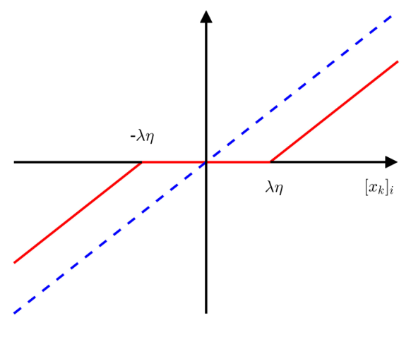
Here is the soft-thresholding operator defined by
| (9) |
where is the -th element of the vector , for . As shown in Fig. 1, once the condition is met, will be penalized to exactly zero, which will remove the corresponding control action and reduce the control depth. The gradient vector is approximated by
| (10) |
in which can be estimated using either classical simulation or quantum hardware. It should be noted that the stop criterion is to continue the iterations until a good-enough threshold value has been reached, and thus whether the expectations are obtained by classical simulation or quantum measurement would not matter. Particularly, the gradient descent update did not use any information of the underlying dynamical model. Therefore, the only consequence brought by realistic noise is that the achieved approximation ratio may be lower than the noise-free case, and gradient estimates may be noisy.
Generally speaking, the convergence rate of cannot be guaranteed in the absence of the convexity assumption on . Nevertheless, since PG descent is a first-order optimization method just as the stochastic gradient descent, its convergence curve is still expected to be stable. In addition, as can be seen from (8), PG descent is simply a reweighting of the conventional gradient descent, which is unlikely to get unstable. Due to these reasons, the stability of the convergence curves can be clearly observed in the numerical results of this paper.
We also consider a second algorithm which does not require to be convex and has a proved convergence rate. This algorithm is an efficient Accelerated Proximal Gradient (APG) descent method proposed in Yao et al. 2017. We can use this unified approach for both convex and non-convex problems to construct the classical optimization part in QAOA. The details are shown in Algorithm 1. It should be noted that the extrapolation defined by step 2 can accelerate the convergence if is locally convex. Steps 3-9 are designed to check if the acceleration works. In step 3, choosing allows to occasionally increase the objective function in order to escape from local minima Grippo and Sciandrone 2002; Yao et al. 2017. In particular, is set to be 2 in the numerical experiments of this paper. Although the only difference between APG and PG appears to be the acceleration part, the convergence rate of APG is shown to be for non-convex Yao et al. 2017.
The regularization parameter in (6) is used to control the model complexity. A large forces most of the elements in to be zero, while a very small results in a model that is close to an unregularized one. For this reason, has to be carefully chosen to encourage a simple control model with sparse while achieving an sufficient level of optimization accuracy. The common practice is to conduct a grid search to find the optimal . In order to mitigate the resource requirement and running time of the algorithm, the candidate hyperparameters can be examined in the following order
| (11) |
That is, the algorithms start with a relatively large , which will produce the most sparse control model. Then the procedures are repeated by decreasing , until a predetermined optimization accuracy has been achieved. Since the regularization strength cannot be too large or too small, only a few s have to be tested before an acceptable result has been obtained, irrespective of problem size. In contrast, the number of experiments needed for finding an optimized depth with random search scales as . Therefore, the automatic algorithm is very efficient when dealing with large-scale problems, where we have .
It should be noted that for the noise-free QAOA considered in this paper, the optimization accuracy always tends to increase with the control depth Farhi et al. 2014; Bengtsson et al. 2020, which means we can always improve the optimization accuracy by decreasing . In that case, the model will become overly complex, or the control depth will become too large. As we have stated, the model complexity can be controlled by selecting the largest that satisfies the criterion (1).
IV Max-Cut and approximation ratio
As a proof-of-principle demonstration, the performance of depth optimization is demonstrated on Max-Cut problem Farhi et al. 2015. Consider an -node non-directed and weighted graph . Max-Cut seeks for a partition of into two subsets and such that the sum of weights of edges connecting nodes in the two disjoint subsets is maximized. By assigning and , the Max-Cut problem can be formulated as a binary optimization
| (12) |
It is known that finding an approximate solution of binary string such that
| (13) |
is NP-hard, with being a minimum ratio Håstad 2001; Zhou et al. 2020. In the QAOA setup, the problem-based Hamiltonian for (12) is given by
| (14) |
The approximation ratio for benchmarking the performance of the QAOA can be defined as
| (15) |
Particularly, maximization the expectation of is equivalent to the minimization of expectation of the following Hamiltonian
| (16) |
for which the approximation ratio can be defined by
| (17) |
with being the theoretical best result. According to (17), the approximation ratio measures the optimization accuracy. In particular, implies that a perfect solution has been obtained by QAOA.
| Vertex | Weight | Vertex | Weight | Vertex | Weight | Vertex | Weight | Vertex | Weight | Vertex | Weight | Vertex | Weight | |
| 7-Node Max-Cut | 0.73 | 0.50 | 0.36 | 0.58 | 0.43 | |||||||||
| 0.33 | 0.69 | 0.88 | 0.67 | |||||||||||
| 10-Node Max-Cut | 0.21 | 0.67 | 0.34 | 0.89 | 0.92 | 0.77 | 0.68 | |||||||
| 0.41 | 0.82 | 0.77 | 0.45 | 0.81 | 0.35 | 0.15 |
V Numerical Results
Two randomly generated instances of Max-Cut for the numerical illustration are given in table 1. The 7-node instance has 9 weighted edges, and the 10-node instance has 14 weighted edges. The code and data for the experiments are available in supplemental material 44 44.
V.1 7-node Max-Cut


First, we demonstrate the performance of depth optimization on the 7-node Max-Cut problem. We let . The elements of and are all initialized as , with an initial control depth of . The minimum acceptable approximation ratio is set to be , which is drawn in red dashed line in Fig. 2. The regularization parameter has four values , which are tested in decreasing order. Note that the effective range of regularization parameter can be estimated based on the range of the objective function and the initial values of the control parameters, as the regularization term has to be comparable with the objective function for the optimization to be successful.
As can be seen in Fig. 2, the depth selection results are consistent for APG and PG with the same . More specifically, the final control depths are basically the same with the same after 200 iterations. Also, it has been shown that if is too large, the algorithms cannot reach the minimum acceptable ratio. The final accuracy is mainly determined by the control depth. That is, the approximation ratios achieved for different algorithms are very close under the same depth, which highlights the importance of depth optimization.
In particular, acceleration in convergence can be observed in Fig. 2(a). APG converges in less than 50 iterations, while PG may need more than 100 iterations to converge. APG achieves the minimum acceptable ratio in about 40 iterations with , and the control depth has been shrunk to 11 at that point. Note that the removal of one control parameter may reduce the number of required control operations by two. For example, if in the control sequence
| (18) |
has been penalized to 0, then the two control operations generated by will be combined into one operation, with a duration of . As a result, the reduction of control depth from to implies a more significant reduction in the number of control operations. As shown in Fig. 3, although the final control depth is , the number of required control operations is only . In this case, the actual percentage of reduction in control operations is that exceeds . Since each unitary control operation is realized as a composition of quantum gates, this reduction in control depth will induce a significant reduction in the number of quantum gates, or the depth of quantum circuit, for practical implementation of QAOA.


The standard practice for model selection is to use the regularized model to solve for the best hyperparameter, and then continue the optimization process without the regularization term to achieve the best accuracy. We have followed this practice and the optimized control sequences are depicted in Fig. 3 and 4. In Fig. 4, the APG and PG algorithms are iterated for 100 times, and then the control depth is fixed for further optimization. It should be noted that the three experiments have achieved basically the same approximation ratio after 300 iterations, which is around 0.9274. This may be because the selected control depth is the same for all three experiments. Started with different values of parameters after the regularization, the ultimate accuracy is still determined by the control depth. In this case, this phenomenon can be taken as evidence to show the importance of optimizing the control depth. Next, we conduct another experiment to show that the performances of APG and PG are not sensitive to small changes in the initial parameters. To do this, the mean and standard derivation of the convergence curves of approximation ratios are calculated with respect to randomly sampled initial values over the interval . As shown in Fig. 5, 100 samples are drawn from a uniform distribution for APG and PG, respectively. The numerical results have confirmed that the convergence of both algorithms are stable against random initialization of parameters.

In Fig. 6, we test the performance of depth optimization by varying the initial control depth, from 20 to 40. For and , the regularization term dominates and the optimized control depths are all similar for different initial values. Even if a large initial value is chosen, the control depth will be automatically reduced to a small value during the iteration, otherwise the regularization term will become too large to optimize. In this case, both the optimized depth and approximation ratio are steady. For and , there is a more subtle trade-off between the regularization term and the objective function. In particular, the control depths are allowed to increase slowly to promote the optimization accuracy. This observation is consistent with the existing conclusion that the optimization accuracy will monotonically increase with the control depth for noise-free QAOA. Specifically, the selected control depth doubled as we increase its initial value from to for . In this case, the regularization strength is too small to penalize the parameters.

| Initial Depth | ||||
| 20 | Length() | 5.36382 | 5.21552 | 4.9451 |
| Depth() | 20 | 19 | 15 | |
| Iterations() | 32 | 27 | 46 | |
| Length(200 iterations) | 6.39597 | 5.11906 | 4.99829 | |
| Depth(200 iterations) | 20 | 14 | 13 | |
| (200 iterations) | 0.9753 | 0.9396 | 0.9120 | |
| 28 | Length() | 8.95274 | 7.02808 | 6.71423 |
| Depth() | 28 | 28 | 26 | |
| Iterations() | 33 | 25 | 30 | |
| Length(200 iterations) | 9.13553 | 6.78664 | 6.51269 | |
| Depth(200 iterations) | 28 | 20 | 18 | |
| (200 iterations) | 0.9882 | 0.9722 | 0.9451 | |
We conduct numerical experiments with initial depths 20, 28 and compare the results of regularized and unregularized cases. The detailed results are shown in Table 2. In this paper, the performance is measured by the model complexity when approximation ratio reaches a desired threshold value. As can be seen from Table 2, the control length, depth and iterations for the regularized models to reach 0.9 are always smaller than the unregularized model, which means that the unregularized model is always the worst and has much room to improve. Even after 200 iterations, the regularized model with still has similar accuracy as the unregularized one, while the control length and depth are significantly reduced under the regularization.
V.2 10-node Max-Cut
For the 10-node instance, the initial control depth is set to be 20. The optimization landscape of 10-node instance is more complex than that of 7-node instance, and thus we choose a smaller learning rate to stabilize the convergence. The initial values for the control parameters are still . The convergence curves for different are plotted in Fig. 7. It can be observed that the performance of APG is unstable at initial stage. In contrast, the convergence of PG is always stable during the iteration. At the initial stage, APG seeks for an acceleration by exploring the optimization landscape with extrapolations. Since bad extrapolations are allowed () in the experiments, the convergence curves can be severely perturbed at initial stage that may cause the objective function to fall into bad local minima. Moreover, the ultimate approximation ratio achieved with APG is slightly worse than PG. This may suggest one has to be cautious with APG in high-dimensional setting due to its indeterministic behaviour in acceleration, although it has a proved convergence rate of .
VI Conclusion
In this paper, we have proposed an automatic and fast algorithm for depth optimization of QAOA based on proximal gradient descent. On one hand, this algorithm can be used as an efficient tool to study the ultimate performances and limitations of QAOA by optimizing the hyperparameter. On the other hand, the automatic algorithm can be directly integrated with quantum hardware to accelerate the optimization process and reduce the control complexity. In particular, the proper control depth can be found with experiments, where is the number of candidate regularization parameters which is small and irrespective of problem size. This results in a significant reduction in the number of experiments for determining the best control depth and approximation ratio, as the number of experiments for finding the best control depth by random search scales with , which could be extremely time-consuming for large-scale problems.
There are two interesting directions for future work. Firstly, due to the inevitable noise in NISQ devices, the optimal control depth could be naturally constrained. As the errors induced by the noise accumulate over time and increase with the control depth, the performance of QAOA may start to decline after the control depth reaches an optimal value. This effect can also be studied by adding noise terms to the ideal quantum dynamical model. For example, it has been found by numerical simulations in Marshall et al. 2020; Alam et al. 2020 that the performance of QAOA may not be monotonically increasing with higher depth when subjected to typical quantum noises. This phenomenon has also been observed in recent experiment Harrigan et al. 2021. In this case, automatic approach may be able to determine the optimal control depth without using the condition (1) for complexity control. Secondly, a dataset can be generated for the depth optimization if robust control is considered. For example, by assuming system uncertainties, a large number of samples can be generated for optimizing the control with respect to a single control task Dong et al. 2020a; Dong et al. 2020b. Clearly, the algorithm proposed in this paper can be extended to realize the robust depth optimization for QAOA. In this case, cross-validation can be used to determine the critical value that maximizes the model generalizability and robustness with a train-test split.
Acknowledgements
This research was supported by the National Natural Science Foundation of China under Grants No. 62173296 and No. 61703364.
References
- Preskill (2018) John Preskill. Quantum Computing in the NISQ era and beyond. Quantum, 2:79, 2018. ISSN 2521-327X.
- Farhi et al. (2014) Edward Farhi, Jeffrey Goldstone, and Sam Gutmann. A quantum approximate optimization algorithm. arXiv:1411.4028, 2014.
- Farhi et al. (2015) Edward Farhi, Jeffrey Goldstone, and Sam Gutmann. A quantum approximate optimization algorithm applied to a bounded occurrence constraint problem. arXiv:1412.6062, 2015.
- Farhi and Harrow (2019) Edward Farhi and Aram W Harrow. Quantum supremacy through the quantum approximate optimization algorithm. arXiv:1602.07674, 2019.
- McClean et al. (2016) Jarrod R McClean, Jonathan Romero, Ryan Babbush, and Alán Aspuru-Guzik. The theory of variational hybrid quantum-classical algorithms. New Journal of Physics, 18(2):023023, 2016.
- Guerreschi and Smelyanskiy (2017) Gian Giacomo Guerreschi and Mikhail Smelyanskiy. Practical optimization for hybrid quantum-classical algorithms. arXiv:1701.01450, 2017.
- Verdon et al. (2019) Guillaume Verdon, Michael Broughton, and Jacob Biamonte. A quantum algorithm to train neural networks using low-depth circuits. arXiv:1712.05304, 2019.
- Wang et al. (2018) Zhihui Wang, Stuart Hadfield, Zhang Jiang, and Eleanor G. Rieffel. Quantum approximate optimization algorithm for maxcut: A fermionic view. Phys. Rev. A, 97:022304, 2018.
- Sweke et al. (2020) Ryan Sweke, Frederik Wilde, Johannes Meyer, Maria Schuld, Paul K. Faehrmann, Barthélémy Meynard-Piganeau, and Jens Eisert. Stochastic gradient descent for hybrid quantum-classical optimization. Quantum, 4:314, 2020. ISSN 2521-327X.
- Liang et al. (2020) Daniel Liang, Li Li, and Stefan Leichenauer. Investigating quantum approximate optimization algorithms under bang-bang protocols. Phys. Rev. Research, 2:033402, 2020.
- Otterbach et al. (2017) J. S. Otterbach et al. Unsupervised machine learning on a hybrid quantum computer. arXiv:1712.05771, 2017.
- Wu et al. (2020) Re-Bing Wu, Xi Cao, Pinchen Xie, and Yu Xi Liu. End-to-end quantum machine learning implemented with controlled quantum dynamics. Phys. Rev. Applied, 14(6):64020, 2020.
- Khairy et al. (2020a) Sami Khairy, Ruslan Shaydulin, Lukasz Cincio, Yuri Alexeev, and Prasanna Balaprakash. Learning to optimize variational quantum circuits to solve combinatorial problems. Proceedings of the AAAI Conference on Artificial Intelligence, 34(03), 2020a.
- Yao et al. (2020) Jiahao Yao, Marin Bukov, and Lin Lin. Policy gradient based quantum approximate optimization algorithm. Proceedings of Machine Learning Research, 107:605–634, 2020.
- Wauters et al. (2020) Matteo M. Wauters, Emanuele Panizon, Glen B. Mbeng, and Giuseppe E. Santoro. Reinforcement-learning-assisted quantum optimization. Phys. Rev. Research, 2:033446, 2020.
- Niu et al. (2019) Murphy Yuezhen Niu, Sirui Lu, and Isaac L. Chuang. Optimizing QAOA: Success probability and runtime dependence on circuit depth. arXiv:1905.12134, 2019.
- Zhou et al. (2020) Leo Zhou, Sheng-Tao Wang, Soonwon Choi, Hannes Pichler, and Mikhail D. Lukin. Quantum approximate optimization algorithm: Performance, mechanism, and implementation on near-term devices. Phys. Rev. X, 10:021067, 2020.
- Larkin et al. (2020) Jason Larkin, Matías Jonsson, Daniel Justice, and Gian Giacomo Guerreschi. Evaluation of QAOA based on the approximation ratio of individual samples. arXiv:2006.04831, 2020.
- Majumdar et al. (2021) Ritajit Majumdar, Dhiraj Madan, Debasmita Bhoumik, Dhinakaran Vinayagamurthy, Shesha Raghunathan, and Susmita Sur-Kolay. Optimizing ansatz design in QAOA for Max-cut. arXiv:2106.02812, 2021.
- R. Herrman and Siopsis (2021) T. S. Humble R. Herrman, J. Ostrowski and G. Siopsis. Lower bounds on circuit depth of the quantum approximate optimization algorithm. Quantum Information Processing, 20(59), 2021.
- Jiang et al. (2017) Zhang Jiang, Eleanor G. Rieffel, and Zhihui Wang. Near-optimal quantum circuit for grover’s unstructured search using a transverse field. Phys. Rev. A, 95:062317, 2017.
- Hastings (2018) Matthew Hastings. Classical and quantum bounded depth approximation algorithms. 2019 Quantum Information & Computation, 19:1116–1140, 2018.
- Bravyi et al. (2020) Sergey Bravyi, Alexander Kliesch, Robert Koenig, and Eugene Tang. Obstacles to variational quantum optimization from symmetry protection. Phys. Rev. Lett., 125:260505, 2020.
- James et al. (2013) Gareth James, Daniela Witten, Trevor Hastie, and Robert Tibshirani. An Introduction to Statistical Learning. Springer-Verlag New York, 2013.
- von Luxburg and Schölkopf (2011) Ulrike von Luxburg and Bernhard Schölkopf. Statistical learning theory: Models, concepts, and results. In Dov M. Gabbay, Stephan Hartmann, and John Woods, editors, Inductive Logic, volume 10 of Handbook of the History of Logic, pages 651–706. North-Holland, 2011.
- Tibshirani (1996) Robert Tibshirani. Regression shrinkage and selection via the lasso. Journal of the Royal Statistical Society. Series B (Methodological), 58(1):267–288, 1996.
- Combettes and Pesquet (2011) Patrick L. Combettes and Jean-Christophe Pesquet. Proximal Splitting Methods in Signal Processing, pages 185–212. Springer New York, New York, NY, 2011. ISBN 978-1-4419-9569-8.
- Beck and Teboulle (2009) Amir Beck and Marc Teboulle. A fast iterative shrinkage-thresholding algorithm for linear inverse problems. SIAM Journal on Imaging Sciences, 2(1):183–202, 2009.
- Li and Lin (2015) Huan Li and Zhouchen Lin. Accelerated proximal gradient methods for nonconvex programming. In Proceedings of the 28th International Conference on Neural Information Processing Systems - Volume 1, page 379–387, 2015.
- Yao et al. (2017) Quanming Yao, James T. Kwok, Fei Gao, Wei Chen, and Tie-Yan Liu. Efficient inexact proximal gradient algorithm for nonconvex problems. In Proceedings of the Twenty-Sixth International Joint Conference on Artificial Intelligence, IJCAI-17, pages 3308–3314, 2017.
- Zou and Hastie (2005) Hui Zou and Trevor Hastie. Regularization and variable selection via the elastic net. Journal of the Royal Statistical Society: Series B (Statistical Methodology), 67(2):301–320, 2005.
- Khairy et al. (2020b) Sami Khairy, Ruslan Shaydulin, Lukasz Cincio, Yuri Alexeev, and Prasanna Balaprakash. Learning to optimize variational quantum circuits to solve combinatorial problems. In Proceedings of the AAAI Conference on Artificial Intelligence, volume 34, pages 2367–2375, 2020b.
- Verstraete et al. (2009) F. Verstraete, M. M. Wolf, and J. I. Cirac. Quantum computation and quantum-state engineering driven by dissipation. Nat. Phys., 5:633–636, 2009.
- Akshay et al. (2020) V. Akshay, H. Philathong, M. E. S. Morales, and J. D. Biamonte. Reachability deficits in quantum approximate optimization. Phys. Rev. Lett., 124:090504, 2020.
- Campos et al. (2021) E. Campos, D. Rabinovich, V. Akshay, and J. Biamonte. Training saturation in layerwise quantum approximate optimization. Phys. Rev. A, 104:L030401, 2021.
- Grippo and Sciandrone (2002) L. Grippo and M. Sciandrone. Nonmonotone globalization techniques for the barzilai-borwein gradient method. Computational Optimization and Applications, 23:143–169, 2002.
- Bengtsson et al. (2020) Andreas Bengtsson, Pontus Vikstål, Christopher Warren, Marika Svensson, Xiu Gu, Anton Frisk Kockum, Philip Krantz, Christian Križan, Daryoush Shiri, Ida-Maria Svensson, Giovanna Tancredi, Göran Johansson, Per Delsing, Giulia Ferrini, and Jonas Bylander. Improved success probability with greater circuit depth for the quantum approximate optimization algorithm. Phys. Rev. Applied, 14:034010, 2020.
- Håstad (2001) Johan Håstad. Some optimal inapproximability results. J. ACM, 48(4):798–859, 2001. ISSN 0004-5411.
- Marshall et al. (2020) Jeffrey Marshall, Filip Wudarski, Stuart Hadfield, and Tad Hogg. Characterizing local noise in QAOA circuits. IOP SciNotes, 1(2):025208, 2020.
- Alam et al. (2020) Mahabubul Alam, Abdullah Ash-Saki, and Swaroop Ghosh. Design-space exploration of quantum approximate optimization algorithm under noise. In 2020 IEEE Custom Integrated Circuits Conference (CICC), pages 1–4, 2020.
- Harrigan et al. (2021) M. P. Harrigan, K. J. Sung, M. Neeley, et al. Quantum approximate optimization of non-planar graph problems on a planar superconducting processor. Nat. Phys., 17:332–336, 2021.
- Dong et al. (2020a) Daoyi Dong, Xi Xing, Hailan Ma, Chunlin Chen, Zhixin Liu, and Herschel Rabitz. Learning-based quantum robust control: Algorithm, applications, and experiments. IEEE Transactions on Cybernetics, 50(8):3581–3593, 2020a.
- Dong et al. (2020b) Yulong Dong, Xiang Meng, Lin Lin, Robert Kosut, and K. Birgitta Whaley. Robust control optimization for quantum approximate optimization algorithms. IFAC-PapersOnLine, 53(2):242–249, 2020b. ISSN 2405-8963. 21st IFAC World Congress.
- (44) See Supplemental Material at URL for code and data for generating figures and tables in this paper.