Joint Spatial Division and Multiplexing for FDD in Intelligent Reflecting Surface-assisted Massive MIMO Systems
Abstract
Intelligent reflecting surface (IRS) is a promising technology to deliver the higher spectral and energy requirements in fifth-generation (5G) and beyond wireless networks while shaping the propagation environment. Such a design can be further enhanced with massive multiple-input-multiple-output (mMIMO) characteristics towards boosting the network performance. However, channel reciprocity, assumed in 5G systems such as mMIMO, appears to be questioned in practice by recent studies on IRS. Hence, contrary to previous works, we consider frequency division duplexing (FDD) to study the performance of an IRS-assisted mMIMO system. However, FDD is not suitable for large number of antennas architectures. For this reason we employ the joint spatial division and multiplexing (JSDM) approach exploiting the structure of the correlation of the channel vectors to reduce the channel state information (CSI) uplink feedback, and thus, allowing the use even of a large number of antennas at the base station. JSDM entails dual-structured precoding and clustering the user equipments (UEs) with the same covariance matrix into groups. Specifically, we derive the sum spectral efficiency (SE) based on statistical CSI in terms of large-scale statistics by using the deterministic equivalent (DE) analysis while accounting for correlated Rayleigh fading. Subsequently, we formulate the optimization problem concerning the sum SE with respect to the reflecting beamforming matrix (RBM) and the total transmit power, which can be performed at every several coherence intervals by taking advantage of the slow-time variation of the large-scale statistics. This notable property contributes further to the decrease of the feedback overhead. Numerical results, verified by Monte-Carlo (MC) simulations, enable interesting observations by elucidating how fundamental system parameters such as the rank of the covariance matrix and the number of groups of UEs affect the performance. For example, the selection of a high rank improves the channel conditioning but increases the feedback overhead.
Index Terms:
Intelligent reflecting surface (IRS), frequency division duplexing (FDD), achievable spectral efficiency, deterministic equivalents, beyond 5G networks.I Introduction
The stringent requirements of fifth-generation (5G) and beyond wireless networks in terms of spectral efficiency (SE) and energy efficiency (EE) could be achieved by relying on disruptive technologies such as intelligent reflecting surface (IRS) and massive multiple-input multiple-output (mMIMO) systems [1, 2, 3]. In particular, IRS has been recently emerged as a revolutionary solution supporting high data rates and low energy consumption [4, 5, 6, 7, 8, 9, 10, 11, 12]. It consists of nearly passive elements, which can create favourable propagation conditions, especially against obstacles, by a smart adjustment of the elements’ phase shifts on the impinging waves. Besides IRS, the mMIMO technology, which has been already deployed in 5G systems [13], assumes a large number of antennas at each base station (BS) by applying low-complexity linear precoding techniques. Among its benefits, we meet high directional beamforming and multiplexing gains while almost cancelling intra-cell interference in the large antenna regime due to channel orthogonality.
With respect to IRS, previous works are classified in two categories depending on whether the phase shifts optimization relies on the instantaneous channel state information (I-CSI) [4, 5, 6] or statistical CSI (S-CSI) [7, 8, 14, 15, 16, 17, 18, 19, 20, 21, 22]. For example, in the first category, requiring optimization at each coherence interval, active and passive beamforming were jointly considered for single cell multi-antenna systems in [4] while the EE maximization problem was addressed in [5].
In the other category, phase shifts, optimized based on S-CSI, do not need to change at every coherence interval but every several intervals. Compared to I-CSI, this method offers lower feedback overhead due to less frequent phase optimization, especially when the numbers of BS antennas and IRS elements are large. Moreover, the feedback overhead reduction results in less power consumption by the IRS controller and release of the capacity requirement for the IRS control link. Furthermore, a significant computational complexity reduction is achieved at the BS, which needs to update the phase shift matrix at a much larger time scale compared to phase shift matrix update in I-CSI schemes that occurs at a much lower frequency. As a result, I-CSI designs could be applied to scenarios with low mobility or fixed location while, in the cases of short coherence intervals such as high mobility environments, phase shifts tuning based on S-CSI tends to be an advantageous solution. On the ground of these benefits, S-CSI design has attracted a lot of interest [7, 8, 14, 15, 16, 17, 18, 19, 20, 21, 22]. For instance, in [8], optimal IRS phase shift design was presented based on maximization of the ergodic rate. Further, in [14], the authors studied IRS-assisted multi-pair systems and applied a genetic algorithm during the phase shifts optimization. Taking into account for random matrix theory, the authors in [18] studied the minimum signal-to-interference-plus-noise ratio (SINR) maximization. In [19], a novel two-timescale beamforming optimization scheme was proposed, where first S-CSI was used to optimize the passive beamforming, and then I-CSI was used to design the active beamforming. In [20], both IRS and additive transceiver hardware impairments (HIs) were studied. Note that IRS HIs appear due to the lack of infinite precision at the IRS phase shifts [23]. In [22], two insightful scenarios, namely, a finite number of large IRS and a large number of finite size IRS were considered towards deriving the coverage probability and it was shown that the latter implementation method is more advantageous.
Although most works have relied on a time division duplex (TDD) design, recent results regarding IRS showed that the phase shifts depend on the angle of the impinging electromagnetic waves, which renders the assumption of channel reciprocity questionable [24, 25, 26]. In particular, in [24], it was shown that channel reciprocity holds only when the incident angles are small while, in [26], several IRS-assisted approaches such as the time-varying control and the structural asymmetries, realizing non-reciprocal channels, were introduced. Hence, the study of the design and the performance of IRS-assisted systems, operating in frequency division duplexing (FDD), is required and is the motivation for the work presented in this paper.11 1 This observation has been also recognised in [25] as one of the most interesting topics for future research. Note that many current wireless networks are based on FDD systems, which contributes further to our interest in such systems. Moreover, FDD operates more effectively in the cases of symmetric traffic and delay-sensitive applications [27]. However, FDD cannot be easily deployed in 5G and beyond systems such as mMIMO because the multi-antenna channel acquisition makes their implementation prohibitive [28]. In particular, FDD includes downlink training, which together with the CSI feedback, present a significant bottleneck as the number of BS antennas increases. Fortunately, the use of the joint spatial division and multiplexing (JSDM) approach allows achieving SE gains similar to mMIMO [29] while it has not been applied yet in IRS systems.
The concept of JSDM relies on the clustering of UEs into groups having approximately the same covariance matrix and the application of dual structured precoding to reduce the feedback overhead efficiently. The structure of the precoder consists of a prebeamforming matrix minimizing the inter-group interference and a linear precoding that depend on large and small-scale fading, respectively. Specifically, the large-scale fading is slowly varying because it depends on the channel second-order statistics such as the channel covariance matrices, which can be acquired accurately with a low feedback overhead while the small-scale fading involves instantaneous CSI. It is worthwhile to mention that the application of JSDM is particularly justified in IRS-assisted systems since a large number of IRS elements results in large dimensional channel matrices that incur further high feedback overhead in FDD IRS systems.
I-A Contributions
The main contributions are summarized as follows.
- •
Contrary to existing works such as [14, 15, 16, 17, 18, 19, 20, 21, 22], which relied on time division duplexing (TDD) transmission for IRS-assisted systems, we consider FDD. To the best of our knowledge, there are no prior works accounting for FDD in IRS and studying its performance except of [30, 31, 32]. Especially, [30] proposed a cascaded codebook and an adaptive bit partitioning strategy, [31] considered a two-way passive beamforming design, and [32] proposed a dimension reduced channel feedback scheme to reduce the channel feedback overhead in RIS assisted systems.
- •
This is the first work applying the concept of JSDM [29] on IRS-assisted systems to reduce the feedback overhead being increasingly significant with the numbers of antennas and IRS elements. In particular, not only do we study the performance but we also provide system guidelines concerning the choice of JSDM parameters. Moreover, we have generalized [29] since we do not assume equal power among the UEs but perform power optimization.
- •
Although many previous works were based on I-CSI knowledge and independent Rayleigh fading such as [4, 5, 6], we move towards consideration of realistic conditions and we hinge on S-CSI (more advantageous) and correlated Rayleigh fading, which is unavoidable as shown in [33]. Remarkably, based on the use of S-CSI and the effective channel, consisting of the cascaded and direct channels, we achieve to obtain the achievable SE of IRS-assisted systems similar to conventional systems. Notably, works considering S-CSI and correlated Rayleigh fading exist (e.g., [18, 19, 20, 22]) but none of them has accounted for the JSDM approach.
- •
By employing the per-group processing (PGP) method of the JSDM approach to reduce the feedback overhead [29], we derive the sum SE of the IRS-assisted mMIMO systems based on FDD in closed-form by leveraging results from the deterministic equivalent (DE) analysis [34, 35, 36]. The importance of the results in terms of DEs is noteworthy since DEs provide an analytical tool resulting in a deterministic expression of the SE based on a convergent system of fixed-point equations while avoiding lengthy Monte Carlo simulations.
- •
We formulate the optimization problem concerning the sum SE subject to reflecting beamforming matrix (RBM) and total transmit power constraints. Note that the PGP method includes the regularized zero-forcing (RZF) precoding and this is the unique work providing RBM optimization based on S-CSI with such a complex precoder. Other works such as [18] considered a simple linear precoding, e.g., maximum ratio transmission (MRT) precoding. Furthermore, the proposed optimization is based on deterministic expressions dependent only on large-scale statistics, and thus, can be performed at every several coherence intervals and reduce considerably the signal overhead as required especially in FDD systems.
- •
We verify the results by Monte-Carlo (MC) simulations and we shed light on the impact of the system parameters on the sum SE such as the signal-to-noise ratio (SNR), the effective covariance rank, the effective channel dimension, and the number of IRS elements. Especially, the effective covariance rank and effective channel dimension play a prominent role by presenting a trade-off between the feedback reduction and the performance.
I-B Paper Outline
The remainder of this paper is organized as follows. Section II presents the system model of an IRS-assisted massive MIMO system with correlated Rayleigh fading operating in FDD and employing the JSDM. Section III provides the asymptotic performance analysis. Section IV presents the sum SE maximization with respect to the IRS RBM and the transmit power. The numerical results are placed in Section V, and Section VI concludes the paper.
I-C Notation
Vectors and matrices are denoted by boldface lower and upper case symbols, respectively. The notations , , and represent the transpose, Hermitian transpose, and trace operators, respectively. The expectation operator is denoted by while represents an diagonal matrix with diagonal elements being the elements of vector . In the case of a matrix , denotes a vector with elements the diagonal elements of . Also, we denote and the notations and with and being two infinite sequences denote almost sure convergence as . The notations and denote the column space of and its orthogonal complement, respectively. Also, the notation denotes the matrix obtained upon removing the th column of , while represents a circularly symmetric complex Gaussian vector with zero mean and covariance matrix . Finally, Table I provides the main abbreviations for the sake of convenience.
| Intelligent reflecting surface | IRS |
|---|---|
| Frequency division duplexing | FDD |
| Time division duplexing | TDD |
| Joint spatial division and multiplexing | JSDM |
| Statistical CSI | S-CSI |
| Instantaneous channel state information | I-CSI |
| Joint spatial division and multiplexing | JSDM |
| Per-group processing | PGP |
| Joint-group processing | JGP |
| Reflecting beamforming matrix | RBM |
| Regularized zero-forcing | RZF |
II System Model
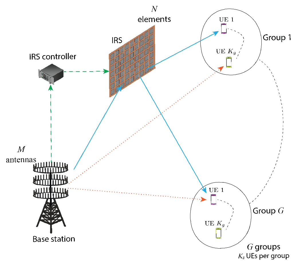
We consider the downlink of an IRS-aided multi-user (MU) multiple-input, single-output (MISO) system with one BS deployed with antennas that serve single-antenna UEs as shown in Fig. 1. Additionally to possibly existing direct links between the BS and the UEs, one IRS, implemented with nearly passive reflecting elements introducing phase shifts onto the impinging signal waves, assists the communication. The size of each IRS element is with and expressing its vertical height and its horizontal width, respectively. The management of the phase shifts takes place by a controller that communicates with the BS through a perfect backhaul link.
As a reasonable design, we assume that the IRS has a line-of-sight (LoS) with the BS. This assumption can be justified by assuming that both the BS and IRS are deployed at high altitude and their locations are fixed. Moreover, we assume that the UEs are spatially clustered into groups each having UEs with the same spatial covariance matrix. The UEs in the same group are nearly co-located while different groups are well-separated. Note that this is a practical assumption since UEs tend to confine in small regions such as buildings. Hence, there exist UEs in total, where the index refers to UEs in group .
II-A Channel and Signal Models
Assuming a flat-fading channel, the received complex baseband signal by the UEs at the th group is given by
| (1) |
where is the channel matrix describing the direct channels between the BS and the UEs in group with being the individual UEs channels. Note that the index denotes UE in group . The subscripts and correspond to the BS-IRS and IRS-UEs links, respectively. Hence, describes the channel between the IRS and the th group with . Also, describes the LoS channel between the BS and the IRS with . Moreover, , satisfying the power constraint , is the linearly precoded transmit signal vector, which means that expresses the transmit SNR. Also, , where expresses the vector of data symbols in group . Note that and with for , where is the linear precoding matrix for group and is the total available transmit power for group with expressing the signal power of UE . The vector expresses the additive white Gaussian noise (AWGN) at the BS. Furthermore, is the diagonal RBM, which expresses the response of the elements with and describing the phase and amplitude coefficient for element , respectively. Henceforth, we make the common assumption of maximum reflection () based on recent advances in lossless metasurfaces [37].
Despite the majority of existing works, e.g., [4, 5], which assumed independent Rayleigh model, we consider the practical effect of spatial correlation, which is unavoidable in realistic IRS-assisted systems [33].22 2 Contrary to most works on IRS that model correlation by using models for conventional antenna arrays, we adopt the recently presented correlation model by the authors in [33], being more suitable for IRS. Also, according to the JSDM method, despite that the individual effects are different across different UEs, the covariances matrices, describing the aggregate result of path-loss and correlation, have been assumed equal across different UEs of the same group since they are clustered accordingly. Thus, and , concerning UE in group , are expressed as
| (2) |
where and represent the deterministic Hermitian-symmetric positive semi-definite aggregate covariance matrices at the BS and the IRS respectively corresponding to group with and . Note that , and , are the path-losses, correlations of the BS-UE and IRS-UE links in group , respectively. This channel modeling is very versatile since it can account for both correlation () and path loss () simultaneously or either of the two. Certain estimation methods (see e.g., [38, 39]) allow to obtain the correlation matrices and the path-losses, which can, thus, be assumed known by the network. Moreover, and express the corresponding fast-fading vectors.
The channel matrix can be expressed as
| . |
Here, is the carrier wavelength, is the path-loss between the BS and the IRS. Also, and are the inter-antenna separation at the BS and inter-element separation at the IRS, respectively [40]. The elevation and azimuth LoS angles of departure (AoD) at the BS with respect to IRS element are described by and . The elevation and azimuth LoS angles of arrival (AoA) at the IRS are described by and . The phases corresponding to the response of the surface elements adjusted in a way so that , which is the necessary condition for supporting multi-stream transmission to the K users of a group. This approach of rank improvement through an intelligent surface has been proposed and validated in [41] for a scenarios with a 2-antenna BS and a 2-antenna UE. In our case, we generalize this approach to a system with an arbitrary number of UEs.
Given the RBM, the overall channel vector between the BS and UE in group is written according to (1) as , which is distributed as with .
It is worthwhile to mention that according to the FDD design with training for channel estimation in both the uplink and the downlink, the following procedure takes place, which consists of two frames. In the uplink frame, each UE first transmits orthogonal pilot symbols to the BS, where these are used to estimate the underlying channels. Following this, all the UEs simultaneously transmit their data to the BS. The data is detected at the BS using the CSI acquired during the pilot transmission phase. During the downlink training frame, the BS transmits orthogonal pilot symbols from its antennas which are used by the UEs to estimate the corresponding downlink channel. These channel estimates are then fed back to the BS by the UEs, and are used by the latter to appropriately precode the data symbols transmitted simultaneously to all the UEs during the data transmission phase.
In terms of implementation, two approaches could be used that present a trade-off between performance and cost. The first approach assumes that makes no compromise on the performance but has a higher cost. It requires IRS elements, where elements are used for the uplink transmission and elements are used for the downlink transmission. The downlink/uplink group of elements operates at the corresponding uplink/downlink frequency. Note that this approach requires all the corresponding hardware to be doubled.33 3 It is true that the gap between the downlink and uplink in 4G/5G systems is not big. It is even lower than 0.3 GHz. For instance, in LTE Band 1 the uplink is defined in the range GHz, whereas the downlink is defined in the range GHz [42]”. Hence the gap between the uplink and downlink is only GHz. However, please have in mind that normally the unit cells of the metasurface that a RIS consists of elements having a narrowband frequency response, unless special designs are manufactured that create a wideband response. For instance, in Section II of [43] it is stated that: “For instance, reflective metasurfaces composed of microstrip patch resonators typically exhibit a fractional bandwidth of less than %.” Even if we assume the worst-case scenario of % fractional bandwidth, this would mean that the frequency response in a downlink FR2 LTE case with carrier frequency GHz is limited in the range GHz GHz, which is smaller than the aforementioned 0.13 GHz gap between the uplink and downlink in LTE. Hence, with the proper design of the intelligent surface unit cells, the frequency response of the unit cells dedicated for the two bands, uplink and downlink, can be such that there is no interference from one band to the other. 44 4 The proposed design concerns 5G and beyond networks, where possibly the frequency interval between the uplink and downlink will be greater than GHz, which is in 4G/5G systems. Hence, there will be no coupling or interference between the uplink and downlink. Despite this, even for smaller intervals, there is no issue because of the following reasons. Doubling the hardware means that there will be separated beamforming networks/control circuits for the uplink RIS and downlink RIS; thus, the uplink RIS and downlink RIS can operate independently. We would like to mention that similar techniques have been well-developed for the phased array design. For example, in [44], an architecture of using a separate transmitter and receiver array operating at GHz is presented. Second, RF filters with high selectivity are used to suppress any unwanted signals from other channels belonging to other frequencies. Without significant performance loss, the whole procedure can be facilitated by the use of diplexers that allow the simultaneous processing of two different frequencies in common FDD systems and also enable the separate phase shifts optimizations that happen during the uplink and downlink transmissions. In particular, the use of radio-frequency (RF)-micro-electromechanical system (MEMS) single-pole double-throw (SPDT) switches to realize phased array transceivers has been well-developed in antenna engineering with applications from microwave frequency to mm-wave frequency ranges. As shown Fig. 2 in [45], the uplink/downlink links, can be realized on a single monolithic microwave integrated circuit (MMIC) with a shared vector modulator (where the phase shifter is located). This well-developed technology is compatible with IRS design and can be applied to IRS to support simultaneous FDD channels. Notably, the switching time of modern SPDT is in the scale of picoseconds. Thus, the uplink and downlink signals can be recovered as far as the speed of the switch can provide enough samples to recover the signals, which is possible according to [45]. Moreover, another technique is through the use of a microwave circulator [46], where the transmit signal will be delivered to the antenna while the received signal from the same antenna will only be delivered to the receiver port.
II-B Advantages/disadvantages of FDD in IRS-assisted systems
FDD has several advantages over TDD that become more pronounced in IRS-assisted systems. For example, FDD design is accompanied with lower latency since communication takes place simultaneously while in TDD there is a switching between transmission and reception. Also, in IRS-assisted systems, where the distance between the transmitter and the receiver is increased, the guard period in TDD systems, being proportional to the distance, increases and affects the performance, while FDD does not appear a problem with large distances. Furthermore, the medium access control (MAC) layer of TDD systems is more complex because it requires accurate time synchronization between uplink and downlink, while FDD systems do not require any uplink/downlink switching mechanism at timescale. However, FDD systems come with higher implementation cost demands such as the diplexers that are required to make the operation in different frequencies possible. Moreover, given that in practical systems, most network volume is consumed in the downlink, in TDD, it is possible to balance the traffic between uplink and downlink by utilising more time slots for downlink. In addition, FDD, using two frequencies instead of one used in TDD, allocates more spectrum.
II-C PGP approach
The JSDM approach was presented in terms of two methods, the joint-group processing (JGP) and PGP [29]. JGP can be applied in the case that the estimation and feedback of the whole matrix from all UEs in all groups are affordable. Normally, the JGP method is accompanied by prohibitive overhead for channel estimation and feedback while PGP is more advantageous due to lower overhead. For this reason, the PGP method, summarized below, is suggested as a more practical approach and is employed in this work.
II-C1 Signal model
PGP suggests a two-stage precoding matrix for group , resulting in feedback overhead and the computational complexity reductions, expressed as
| (3) |
where is the preprocessing matrix based on the long-term channel statistics with being an integer parameter to be optimized. Also, , is the precoding matrix based on the instantaneous channel (short-term CSI) of group .
Hence, the received signal in (1) with dual precoding described by (3) can be written as
| (4) |
where .
Based on the Karhunen-Loeve representation, the channel vector can be written as
| (5) |
where is a tall unitary matrix including the eigenvectors of that correspond to the non-zero eigenvalues, is an diagonal matrix with elements the non-zero eigenvalues of , and . Generally, . Thus, we have .
II-C2 Imperfect CSI
Certain reasons such as quantization can result in imperfect feedback of the CSI to the BS (see Rem. 1 below), which is accompanied with significant overhead. Especially, the imperfect CSI at the BS from group can be expressed as
| (6) |
where is the perfect CSI and with denoting the corresponding error that consists of elements with zero mean and unit variance. The parameter describes the accuracy of the available CSI in group . Hence, if , we obtain perfect CSI while implies no CSI knowledge. Without loss of generality, we assume that the levels of CSI accuracy for all groups are the same, i.e., . From (6), can be defined as the imperfect CSI knowledge of by using . Note that the imperfect CSI , given in terms of is based on a given RBM. The assumption of a fixed RBM during one coherence interval is justified based on the fact that RBM is expected to change according to large-scale statistics expressed by , which changes at every several coherence intervals.
Remark 1
Having assumed that both the BS and UEs are aware of large-scale statistics, the model in (6) can describe the scenario, where the th UE in the group quantizes with the help of a random codebook and sends back the codeword index to the BS [28]. We provide an example of the advantage of using this method in Sec. V.
II-C3 Design of pre-beamforming
Using block diagonalization (BD) preprocessing to cancel out the inter-group interference, we design the pre-beamforming matrix as
| (7) |
where the index corresponds to group . In the case of exact BD, (4) becomes
| (8) |
Exact BD can be achieved, if while the necessary multiplexing gain can be achieved if for all groups . In other words, for given sets of and satisfying , can be designed if for all and . If the dimension of is less than , the rank condition is not fulfilled. In such case, there are two options: i) reduction of , or ii) resort to approximate BD.
Herein, we choose approximate BD to design . For this reason, we choose dominant eigenvalues of . On this ground, we write , where is the matrix consisted of the dominant eigenvectors and is the matrix including the eigenvectors corresponding to the weakest eigenvalues. To achieve approximate BD, we have to choose the dominant eigenmodes for each group subject to the condition for all groups . Notably, the design of has to take into account a feasible choice of the parameters , , and that should be optimized to maximize the SE under a given system setup. The matrix is constructed as in [29]. Herein, we briefly summarize the main steps. Hence, first, we define the matrix
| (9) |
whose size is and its rank is . Based on SVD, let a set of left eigenvectors of denoted by , where expresses the left singular vectors corresponding to the dominant singular values while corresponds to the left singular vectors with non-dominant singular values . Now, we define the matrix , which has the property to be orthogonal to the dominant eigenspace spanned by the channel of other groups. The covariance matrix of is given by
| (10) | ||||
| (11) | ||||
| (12) |
where (11) is based on (5) while (12) is the SVD of , i.e., describes the eigenvectors of . The pre-beamforming matrix is obtained by setting , where corresponds to the dominant eigenmodes of . In particular, we have that
| (13) |
which means that coincides with the dominant eigenmodes of while it is orthogonal to the dominant eigenmodes of groups . Gathering all constraints, the condition , where should be satisfied.
III Asymptotic Performance Analysis with Dual Precoding
In this section, we first provide the analysis towards the derivation of the downlink achievable SE of IRS-assisted systems based on FDD while employing the JSDM method in the case of the PGP approach.
The derivation of the DE SINR requires the following assumptions concerning the correlation matrices and the power allocation matrix as in [34].
Assumption 1
All correlation matrices, i.e., and have uniformly bounded spectral norm on and , respectively, i.e.,
| (14) |
Assumption 2
The maximum power of group , i.e., is of the order , being equivalent to
| (15) |
According to (4), the effective channel of group is with covariance matrix for UE being . For the sake of exposition, we assume the same number of dominant eigenvalues per group, the same number of UEs per group, and the same dimension of the pre-beamforming matrix per group, i.e., , , and . The extension to the general case is immediate and straightforward. Hence, the dimensions of are . The precoding matrix for group is designed in terms of the instantaneous imperfect CSI to cancel out the intra-group interference on that group as
| (16) |
where with being the effective channel estimate at the BS while is the imperfect CSI knowledge of . Also , selected as to be equivalent with the RZF linear filter [47], is a regularization factor that makes expressions converge to a constant, and is the normalization parameter that fulfils the power constraint for group . In particular, the normalization parameter becomes
| (17) | ||||
| (18) |
where (17) is obtained because as the product of two tall matrices. Hence, based on (4) and (18), the SINR of the th UE in group with perfect receiver CSI is given by
| (19) |
where
| (20) | ||||
| (21) | ||||
| (22) |
with the numerator expressing the desired signal power while the first and second terms in the denominator express the self-group and inter-group interferences, respectively.
Under the Assumptions 1-2 and by assuming that while , , and also go to infinity by keeping their ratio with fixed, the DE SINR fulfils
| (23) |
Theorem 1
The DE of the downlink SINR of UE with PGP in IRS-assisted mMIMO systems with FDD, accounting for imperfect CSI, is given by
| (24) |
where and with .
The expressions of , , , are the unique solutions of
| (25) | ||||
| (26) | ||||
| (27) | ||||
| (28) |
Proof:
The proof is provided in Appendix A.∎
Based on the dominated convergence [48] and the continuous mapping theorem [49], the DE of the sum-rate is given by
| (29) |
where
The nature of the multicast mechanism indicates that the DE sum-rate of group , allocated with total power such that , is determined by , where is the DE rate of UE in group .
Proposition 1
In IRS-assisted mMIMO systems with PGP, all UEs in group are allocated with equal power and the DE sum-rate of group is since all these UEs have equal achievable rate .
IV Sum SE Maximization Design
In this section, we perform optimization of sum SE of the overall IRS-assisted mMIMO system. In particular, the sum-rate maximization problem is expressed as follows
| (31a) | ||||
| (31b) | ||||
| (31c) | ||||
where constraint (31b) guarantees that the BS transmit power is kept below the maximum power and constraint (31c) expresses that each IRS element results in only a phase shift without any amplification of the incoming signal. Note that for the sake of exposition, we have defined the vector and for all corresponding to the elements of .
Corollary 2
Let , then does not depend on . Equivalently, is independent on the phase shifts, and thus, cannot be optimized in this case.
The optimization problem is non-convex and subject to a unit-modulus constraint regarding , which make its solution challenging. To address this, we rely on the common approach in IRS literature, being the application of the alternating optimization (AO) technique, where and are going to be solved separately and iteratively. Hence, first, we solve for given a fixed . Next, we focus on finding the optimum with fixed. The iteration of this process achieves the increase of at each iteration step until convergence of the objective to its optimum value since it is upper-bounded due to the power constraint (31b).
IV-A IRS Design
So far, we have considered the RBM fixed. However, to exploit the IRS towards the maximization of the sum SE, the RBM has to be optimized. Notably, we observe its presence inside the covariance matrices that appear in the DE expression of the SE with PGP. By assuming infinite resolution phase shifters and under imperfect CSI conditions, the RBM optimization problem for single-cell FDD systems employing the JSDM method is formulated as
| (32) | ||||
where is given by (31a). The maximization problem is non-convex with respect to while it is subject to a unit-modulus constraint regarding . A local optimal solution to this problem can be obtained by applying the projected gradient ascent algorithm until converging to a stationary point, which means that, at every step, we project the solution onto the closest feasible point satisfying the unit-modulus constraint concerning [18]. Specifically, at step , the phases are included in the vectors . The next step of the iteration towards convergence increases , and is described by
| (33) |
where the parameter describes the step size and expresses the ascent direction at step . For the computation of the suitable step size at each iteration, we apply the backtracking line search [50]. Note that is provided by Proposition 2 below. The projection problem under the unit-modulus constraint provides the solution of the problem described by (33). In Algorithm 1, we present the outline of this procedure.
1. Initialisation: , , given by (31a);
2. Iteration : for do
3. , where is given by Proposition 2;
4. Find by backtrack line search [50];
5. ;
6. ; ;
7. ;
8. Until ; Obtain ;
9. end for
Proposition 2
The derivative of with respect to is provided by
| (34) |
where
| (35) | ||||
| (36) |
with
| (37) | ||||
| (38) | ||||
| (39) | ||||
| (40) | ||||
| (41) | ||||
| (42) |
with
| (43) |
and for written as where each term is computed by Lemma 2. The expressions of , , , and , given in Theorem 1 and Corollary 1 together with , , , , , , and are obtained by solving the system of fixed-point equations (25)-(28), (38)-(42).
Proof:
The proof is given in Appendix C.∎
The RBM beamforming design is based on the gradient ascent and offers a significant advantage because the gradient ascent is derived in a closed-form. Note that it has low computational complexity because it consists of simple matrix operations. Specifically, the complexity of (35) is . Obviously, the derivative is a function of the fundamental system parameters , , and with the number of IRS elements having the higher (square) impact.
IV-B Power Allocation Optimization
Now, for a fixed RBM , the objective is the optimization over . In particular, we have
| (44) | ||||
where is given by (31a). This problem is not convex but a local optimal solution can be obtained by using a weighted minimum mean square error (WMMSE) reformulation of the sum SE maximization. By denoting , the SINR can be expressed as a function of the downlink power coefficients given by the vector as
| (45) |
where
| (46) | ||||
| (47) | ||||
| (48) |
Now, the optimization problem becomes
| (49) | ||||
For the MMSE reformulation, we assume the single-input and single-output (SISO) channel that corresponds to this SINR given by
| (50) |
where is the received signal, denotes the normalized and independent random data signal with , and . In such case, the receiver can compute an estimate of the desired signal , where as a scalar combining coefficient. The resulting MSE is written as
| (51) |
The coefficient , minimizing the MSE for a given , becomes
| (52) |
Plugging into (51), becomes . Based on the weighted MMSE method, we introduce the auxiliary weight for the MSE and solve the following problem
| (53) | ||||
Note that both and are equivalent, meaning that they have the same optimal solution. The equivalence stems from the fact that the optimal in (53) is . The advantage of the reformulation results in the following lemma adapted from [51, Th. 3].
Lemma 1
The block descent coordinate algorithm, provided in Algorithm 2, converges to a local optimum of in terms of AO among three blocks of variables , , and .
Algorithm 2 describes the whole procedure for the power optimization and Step includes a subproblem that needs to be solved in every iteration. It can be solved in closed-form as
| (55) |
where are treated as optimization variables. Basically, the problem is decomposed into independent subproblems, where each one of them concerns a quadratic minimization under a bound constraint.
The power allocation presents a similar complexity to the RBM design since Algorithm 2 consists of similar matrix operations, i.e., its complexity is .
V Numerical Results
In this section, we elaborate on the numerical results of the sum SE in IRS-assisted systems under the FDD protocol by applying PGP of the JSDM method. MC simulations in terms of independent channel realizations verify the deterministic equivalent analysis.
The simulation setup includes a uniform linear array (ULA) of antennas at the BS, which serves UEs while aided by an IRS with a uniform planar array (UPA) of elements. UEs are equally shared among groups, which means that each group consists of UEs. The correlation matrices and are obtained similar to [35] and [33], respectively. Note that the size of each IRS element is given by . Furthermore, the path-losses for the BS-to-IRS and IRS-to-UE links are given by [4, 18]
| (56) |
where and are the path-loss exponent and distance concerning the former link while and are the path-loss exponent and distance concerning the latter link. In the case of , we assume the same parameters as for , and additionally, we consider a penetration loss of . The choice of these values relies on the 3GPP Urban Micro (UMi) scenario from TR36.814 for a carrier frequency of GHz and a noise level of dBm. Especially, the path-losses for and are generated according to the LOS and NLOS versions [52]. Also, dB and dB, which are the path-losses at a reference distance of m while each UE includes a single 0dBi antenna [53]. Also, we have chosen and . The latter value is justified because under these setting the rank of the channel covariance matrix is while only of them are important. Unless otherwise stated, this set of parameters values is used during the simulations. Note that , where .
Figs. 2.(a) and 2.(b) illustrate the impact of the effective rank of the channel covariance matrix of each group on the performance of JSDM in IRS-assisted systems in the cases of perfect and imperfect CSI. Under perfect CSI conditions ("solid" lines) with , we notice that in the case of choosing (Fig. 2.(a)), PGP saturates at high SNR since this effective rank value is too small. In particular, such a choice does not allow for consideration of the substantial eigenmodes by the pre-beamforming matrix and results in large inter-group interference. On the contrary, a better (higher) choice for , i.e., (see Fig. 2.(b)) allows the inclusion of the significant eigenmodes and no interference-limited behaviour is noticed until dB. Of course, the rate saturates at some larger SNR, belonging outside the scope of practical applications. Obviously, the choice of the rank value depends on the channel covariance matrix. In the case of imperfect CSI (), met in practice, saturation is observed in both figures ("dashed" lines). However, when we have , the saturation starts much earlier ( dB) while a choice of (Fig. 2.(b)) is more robust regarding the performance since the saturation is encountered after dB. Similar observations hold when . The inference from these two figures is that a good selection of , where the major eigenmodes are taken into account, defines the performance. A small value results in severe performance degradation while a value close to the full rank will result in a dimensionality bottleneck while not achieving any profit concerning the interference. In these figures, we also show the degradation of the sum SE when no correlation ("dotted" lines) is taken into account because in such a case the IRS cannot be optimized.
To elaborate further on the saving advantage of the JSDM method, we would like to highlight that after the downlink training of all groups () with effective channel dimension , each of the UEs in each group has to feedback its channel vector, which equals to quantized complex channel coefficients.55 5 This conclusion assumes that downlink training has already taken place at some previous stage. Note that this work does not perform downlink training but this task and its effects are left for future study. However, in this case, where the BS is deployed with antenna aimed at serving UEs in total, orthogonal downlink training symbols are required while a total of channel coefficients will be fed back, which means the achievement of saving by a factor of .


In Fig. 3, we depict the impact of the parameter for a specific and when (imperfect CSI) for varying SNR values, being dB. Specifically, after selecting according to the discussion in the previous paragraph and subject to the constraint , we observe that the sum SE does not increase monotonically but there is an optimal value because its increase results in a trade-off between a larger dimensionality overhead and a better channel conditioning. Moreover, we observe that the higher the SNR, the smaller the optimal becomes. Also, we notice that at higher SNR, the range of sum SE values takes higher values but the impact of variation is smaller with increasing SNR as witnessed by the slopes of the corresponding lines.

Fig. 4 shows the achievable sum SE versus the number of BS antennas for both perfect and imperfect CSI, when elements. We observe that exhibits a similar dependence on as on in the previous figure. Thus, when grows large, the sum SE increases without limit in both cases of perfect and imperfect CSI. In general, these two figures indicate that an IRS-assisted system performs better with larger values of IRS elements and BS antennas. In particular, the latter is further interesting because it agrees with the massive MIMO design trend that has already started to be implemented. In addition, we verify that the performance increases in the presence of the IRS.
Fig. 5 illustrates the achievable sum SE versus the number of IRS elements for both cases of perfect and imperfect CSI, when antennas. We notice that the sum SE increases with the increasing number of IRS elements in both cases, but the increase is slower in the case of imperfect CSI. Also, disregarding the IRS size, defined by its elements, it always provides better performance compared to its absence. In other words, its application is beneficial because it results in a further enhancement of the channel additionally to the direct signal. Moreover, we consider the scenario of "random" phase shifts and we show that the RBM optimization enhances significantly the performance.


Fig 6 depicts the sum SE versus the number of groups in the case of imperfect CSI () while varying the effective rank , the effective channel dimension , and UEs per group . We notice that the sum SE increases with the number of groups but this increase becomes slower when the number of UEs per group grows due to increased multiuser interference while the rest of the parameters are the same. In addition, for a specific , an increase of the channel rank results in an increase of the sum SE but caution should be taken since the overhead (dimensionality) increases too. Moreover, by increasing , the sum SE increases until a specific equal to while keeping increasing results in lower sum SE due to larger dimensionality cost again.


Fig. 7.(a) illustrates the convergence of the proposed overall algorithm based on AO, which consists of the subproblems of RBM and transmit power optimizations. Specifically, we have depicted the sum SE versus the number of iterations for varying numbers of IRS elements and UE groups. As can be seen, the convergence of the optimization is fast in all cases, where the algorithm has converged at most in iterations (see the "dashed-square" line). Also, as expected, as the number of IRS elements and groups increases, more iterations are needed until convergence since the number of optimization variables has increased.
The non-convexity of the overall optimization problem suggests that its solution depends on the initial point, i.e., different initial points result in different locally optimal solutions. Fig. 7.(b) investigates this dependence on the initializations by accounting for channel realizations. The initialization of the overall algorithm including Algs. and assumes that and as mentioned previously. "Alg. 1-Test" in the figure assumes the best initial point out of random initial points for each channel instance. We observe indeed that different initializations result in different solutions and that the sum SE in both cases is almost the same, which means that this phase shifts selection for initialization is a good choice.
VI Conclusion
In this paper, we tackled the channel non-reciprocity witnessed in IRS-assisted communication systems. For this reason, we assumed an mMIMO system assisted with an IRS operating in FDD. To this end, we applied the JSDM method by grouping the UEs with the same covariance matrix to improve the performance, which, otherwise, would be afflicted due to prohibitive feedback overhead as the number of BS antennas and IRS elements increases. Based on DE tools and S-CSI knowledge, we derived the sum SE accounting for correlated Rayleigh fading. Next, we formulated the optimization problem maximizing the sum SE under RBM and power budget constraints. To solve the nonconvex optimization, we proposed an efficient AO algorithm that can be performed at every several coherence intervals, which results in further reduction of the feedback overhead and computational complexity. Among the observations, we would like to highlight that the rank of the covariance matrix is a crucial parameter having a direct impact on the performance. Its increase improves the performance due to better channel conditioning while it burdens the feedback overhead. Other interesting directions could be the extension of this work to account for 3-dimensional beamforming with multiple beams in the elevation angle and the consideration of multiple distributed IRS.
Appendix A Proof of Theorem 1
The derivation of the DE SINR is obtained by following the approach in [34] but with extension to imperfect CSI that brings considerable differences. Hence, taking into account for imperfect CSI, the proof consists of the derivation of the DEs of four parts: i) The power normalization term , ii) the desired signal power part , iii) the self-group interference power part , and iv) the inter-group interference power part .
Regarding , we have
| (57) | ||||
| (58) | ||||
| (59) | ||||
| (60) |
where . In (58), we applied the matrix inversion lemma twice [35, Lem. 1] and, in (59), we used [35, Lem. 4]. The last step makes use of [35, Th. 1] with and defined in Theorem 1. Note that is basically the derivative of with respect to , i.e., , where . Its expression is obtained after some algebraic manipulations.
In the case of , we have
| (61) | ||||
| (62) | ||||
| (63) |
where in (61), we applied the matrix inversion lemma [35, Lem. 1], and, in (62), we used (6). In (63), we used [35, Lem. 4] by considering the independence between and . Next, we applied [35, Lem. 4], [35, Lem. 3], and [35, Th. 1].
For , we have
| (64) | ||||
| (65) |
In (64), we used that , where with , , and . In (65), we denoted . Similar to previous derivations, we obtain
| (66) | ||||
| (67) | ||||
| (68) | ||||
| (69) |
where . Hence, we have almost surely that
| (70) | ||||
| (71) |
where (70) reduces to (71) after proper substitutions. Based on the rank perturbation lemma [35, Lem. 3], we have
| (72) |
Also, we denote , where , which can be written as
| (73) |
after applying [35, Lems. 1, 4, 3]. Note that
| (74) |
where
| (75) | ||||
| (76) |
with being the derivative at . Use of (76) into (74) and substitution into (73) gives .
The derivation of follows similar lines with . In this case, is obtained as given in Theorem 1. Having obtained all terms in the SINR, the proof is concluded.
Appendix B Proof of Proposition 1
The power optimization problem for group is formulated as
| (77) | ||||
where does not depend on UE . The solution to is obtained by the water-filling algorithm as
| (78) |
where is a parameter defining the water level to satisfy the constraint [54]. Since is identical for all UEs in group , the optimal powers, maximizing , are all equal and given by . In such case, all user rates of group become equal to and the sum-rate of this group becomes .
Appendix C Proof of Proposition 2
First, we present the following lemma, which is required in the following derivations.
Lemma 2
The derivative of the trace including the covariance matrix and the matrix with respect to , where is independent of , is given by
| (79) |
Proof:
Hereafter, we denote the partial derivative with respect to by . Starting from the gradient of , with respect to , which relies on the quotient rule derivative, we obtain
| (83) |
where the calculation of the partial derivatives follows. In particular, is written as
| (84) |
where
| (85) |
with , being the derivative of an inverse matrix obtained by [55, Eq. 40] as . The derivative of is given by
| (86) |
where is the derivative of with respect to whose trace expression is given by Lemma 2. As a result, after substituting (85)-(86) into (84), we obtain .
The derivative of is given by
| (87) |
where
| (88) | ||||
| (89) |
are derived easily by applying basic derivative rules. For the derivatives of , , and , we notice that that they have a similar expression. Thus, we resort to the definition of a new function , which includes them under specific values of its parameters and , and we compute its derivative. Thus, by defining
| (90) |
we have , , and . Note that the dependence on the RBM is found on while appears no such dependence. Also, we define . After some lengthy algebraic manipulations, we obtain in (43), where for written as with given above while the derivatives of the traces are obtained by using Lemma 2. Hence, after suitable substitutions in (43), we obtain , , and .
References
- [1] J. Zhang et al., “Prospective multiple antenna technologies for beyond 5G,” IEEE J. Sel. Areas Commun., vol. 38, no. 8, pp. 1637–1660, 2020.
- [2] T. L. Marzetta et al., Fundamentals of Massive MIMO. Cambridge University Press, 2016.
- [3] Q. Wu and R. Zhang, “Towards smart and reconfigurable environment: Intelligent reflecting surface aided wireless network,” IEEE Commun. Mag., vol. 58, no. 1, pp. 106–112.
- [4] Q. Wu and R. Zhang, “Intelligent reflecting surface enhanced wireless network via joint active and passive beamforming,” IEEE Trans. Wireless Commun., vol. 18, no. 11, pp. 5394–5409, 2019.
- [5] C. Huang et al., “Reconfigurable intelligent surfaces for energy efficiency in wireless communication,” IEEE Trans. Wireless Commun., vol. 18, no. 8, pp. 4157–4170, 2019.
- [6] C. Pan et al., “Multicell MIMO communications relying on intelligent reflecting surfaces,” IEEE Trans. Wireless Commun., vol. 19, no. 8, pp. 5218–5233, 2020.
- [7] H. Guo et al., “Weighted sum-rate maximization for reconfigurable intelligent surface aided wireless networks,” IEEE Trans. Wireless Commun., vol. 19, no. 5, pp. 3064–3076, 2020.
- [8] Y. Han et al., “Large intelligent surface-assisted wireless communication exploiting statistical CSI,” IEEE Trans. Veh. Tech., vol. 68, no. 8, pp. 8238–8242, 2019.
- [9] A. M. Elbir et al., “Deep channel learning for large intelligent surfaces aided mm-Wave massive MIMO systems,” IEEE Wireless Commun. Lett., vol. 9, no. 9, pp. 1447–1451, 2020.
- [10] Y. Yang et al., “Intelligent reflecting surface meets OFDM: Protocol design and rate maximization,” IEEE Trans. Commun., vol. 68, no. 7, pp. 4522–4535, 2020.
- [11] Q. Wu and R. Zhang, “Joint active and passive beamforming optimization for intelligent reflecting surface assisted SWIPT under QoS constraints,” IEEE J. Sel. Areas Commun., vol. 38, no. 8, pp. 1735–1748, 2020.
- [12] W. Tang et al., “Wireless communications with reconfigurable intelligent surface: Path loss modeling and experimental measurement,” IEEE Trans. Wireless Commun., vol. 20, no. 1, pp. 421–439, 2021.
- [13] P. von Butovitsch et al., “Advanced antenna systems for 5G networks,” Ericsson White Paper.
- [14] Z. Peng et al., “Analysis and optimization for IRS-aided multi-pair communications relying on statistical CSI,” arXiv preprint arXiv:2007.11704, 2020.
- [15] G. Yu et al., “Design, analysis, and optimization of a large intelligent reflecting surface-aided B5G cellular internet of things,” IEEE Int. Things J., vol. 7, no. 9, pp. 8902–8916, 2020.
- [16] X. Hu et al., “Location information aided multiple intelligent reflecting surface systems,” IEEE Trans. Commun., vol. 68, no. 12, pp. 7948–7962, 2020.
- [17] Q.-U.-A. Nadeem, A. Chaaban, and M. Debbah, “Opportunistic beamforming using an intelligent reflecting surface without instantaneous CSI,” IEEE Wireless Commun. Lett., vol. 10, no. 1, pp. 146–150, 2021.
- [18] A. Kammoun et al., “Asymptotic max-min SINR analysis of reconfigurable intelligent surface assisted MISO systems,” IEEE Trans. Wireless Commun., vol. 19, no. 12, pp. 7748–7764, 2020.
- [19] M.-M. Zhao et al., “Intelligent reflecting surface enhanced wireless network: Two-timescale beamforming optimization,” IEEE Trans. Wireless Commun., vol. 19, no. 8, pp. 5218–5233, 2020.
- [20] A. Papazafeiropoulos et al., “Intelligent reflecting surface-assisted MU-MISO systems with imperfect hardware: Channel estimation, beamforming design,” IEEE Trans. Wireless Commun., 2021.
- [21] T. Van Chien et al., “Outage probability analysis of IRS-assisted systems under spatially correlated channels,” IEEE Wireless Commun. Lett., pp. 1–1, 2021.
- [22] A. Papazafeiropoulos et al., “Coverage probability of distributed IRS systems under spatially correlated channels,” IEEE Wireless Commun Lett., pp. 1–1.
- [23] M.-A. Badiu and J. P. Coon, “Communication through a large reflecting surface with phase errors,” IEEE Wireless Commun. Lett., vol. 9, no. 2, pp. 184–188, 2019.
- [24] W. Chen et al., “Angle-dependent phase shifter model for reconfigurable intelligent surfaces: Does the angle-reciprocity hold?” IEEE Commun. Lett., vol. 24, no. 9, pp. 2060–2064, 2020.
- [25] C. Pan et al., “Reconfigurable intelligent surfaces for 6G systems: Principles, applications, and research directions,” IEEE Commun. Mag., 2021.
- [26] W. Tang et al., “On channel reciprocity in reconfigurable intelligent surface assisted wireless network,” arXiv preprint arXiv:2103.03753.
- [27] Z. Jiang et al., “Achievable rates of FDD massive MIMO systems with spatial channel correlation,” IEEE Trans. Wireless Commun., vol. 14, no. 5, pp. 2868–2882, 2015.
- [28] N. Jindal, “MIMO broadcast channels with finite-rate feedback,” IEEE Trans. Inf. Theory, vol. 52, no. 11, pp. 5045–5060, 2006.
- [29] A. Adhikary et al., “Joint spatial division and multiplexing-The large-scale array regime,” IEEE Trans. Inf. Theory, vol. 59, no. 10, pp. 6441–6463, 2013.
- [30] W. Chen et al., “Adaptive bit partitioning for reconfigurable intelligent surface assisted FDD systems with limited feedback,” arXiv preprint arXiv:2011.14748, 2020.
- [31] B. Guo, C. Sun, and M. Tao, “Two-way passive beamforming design for RIS-aided FDD communication systems,” in 2021 IEEE Wireless Commun. Net. Conf. (WCNC). IEEE, 2021, pp. 1–6.
- [32] D. Shen and L. Dai, “Dimension reduced channel feedback for reconfigurable intelligent surface aided wireless communications,” IEEE Trans. Commun., vol. 69, no. 11, pp. 7748–7760, 2021.
- [33] E. Björnson and L. Sanguinetti, “Rayleigh fading modeling and channel hardening for reconfigurable intelligent surfaces,” IEEE Wireless Commun. Lett., vol. 10, no. 4, pp. 830–834, 2021.
- [34] S. Wagner et al., “Large system analysis of linear precoding in correlated MISO broadcast channels under limited feedback,” IEEE Trans. Inf. Theory, vol. 58, no. 7, pp. 4509–4537, July 2012.
- [35] J. Hoydis, S. ten Brink, and M. Debbah, “Massive MIMO in the UL/DL of cellular networks: How many antennas do we need?” IEEE J. Select. Areas Commun., vol. 31, no. 2, pp. 160–171, February 2013.
- [36] A. K. Papazafeiropoulos and T. Ratnarajah, “Deterministic equivalent performance analysis of time-varying massive MIMO systems,” IEEE Trans. Wireless Commun., vol. 14, no. 10, pp. 5795–5809, 2015.
- [37] T. Badloe, J. Mun, and J. Rho, “Metasurfaces-based absorption and reflection control: Perfect absorbers and reflectors,” J. of Nanomaterials, vol. 2017, 2017.
- [38] D. Neumann, M. Joham, and W. Utschick, “Covariance matrix estimation in massive MIMO,” IEEE Signal Process. Lett., vol. 25, no. 6, pp. 863–867, 2018.
- [39] K. Upadhya and S. A. Vorobyov, “Covariance matrix estimation for massive MIMO,” IEEE Signal Process. Lett., vol. 25, no. 4, pp. 546–550, 2018.
- [40] Q. Nadeem et al., “Intelligent reflecting surface-assisted multi-user MISO Communication: Channel estimation and beamforming design,” IEEE Open J. Commun. Soc., vol. 1, pp. 661–680, 2020.
- [41] Ö. Özdogan, E. Björnson, and E. G. Larsson, “Using intelligent reflecting surfaces for rank improvement in MIMO communications,” in ICASSP 2020-2020 IEEE International Conference on Acoustics, Speech and Signal Processing (ICASSP). IEEE, 2020, pp. 9160–9164.
- [42] U. E. U. conformance specification Radio, “3rd generation partnership project; Technical Specification Group Radio Access Network; Evolved Universal Terrestrial Radio Access (E-UTRA); User Equipment (UE) conformance specification radio transmission and reception.”
- [43] X. You, C. Fumeaux, and W. Withayachumnankul, “Tutorial on broadband transmissive metasurfaces for wavefront and polarization control of terahertz waves,” J. Applied Physics, vol. 131, no. 6, p. 061101, 2022-02. [Online]. Available: https://doi.org/10.1063/5.0077652
- [44] W. Lee et al., “Fully integrated 94-GHz dual-polarized TX and RX phased array chipset in SiGe BiCMOS operating up to C,” IEEE J. Solid-State Circuits, vol. 53, no. 9, pp. 2512–2531, 2018.
- [45] T. Chaloun et al., “Wide-angle scanning active transmit/receive reflectarray,” IET Microwaves, Antennas & Propagation, vol. 8, no. 11, pp. 811–818, 2014.
- [46] T. Dinc, A. Nagulu, and H. Krishnaswamy, “A millimeter-wave non-magnetic passive SOI CMOS circulator based on spatio-temporal conductivity modulation,” IEEE J. Solid-State Circuits, vol. 52, no. 12, pp. 3276–3292, 2017.
- [47] D. Tse and P. Viswanath, Fundamentals of wireless communication. Cambridge university press, 2005.
- [48] P. Billingsley, Probability and measure, 3rd ed. John Wiley & Sons, Inc., 2008.
- [49] A. W. van der Vaart, Asymptotic statistics (Cambridge series in statistical and probabilistic mathematics). New York: Cambridge University Press, 2000.
- [50] S. Boyd, S. P. Boyd, and L. Vandenberghe, Convex optimization. Cambridge university press, 2004.
- [51] Q. Shi et al., “An iteratively weighted MMSE approach to distributed sum-utility maximization for a MIMO interfering broadcast channel,” vol. 59, no. 9, pp. 4331–4340, 2011.
- [52] E. Access, “Further advancements for E-UTRA physical layer aspects,” 3GPP Technical Specification TR, vol. 36, p. V2, 2010.
- [53] E. Björnson, Ö. Özdogan, and E. G. Larsson, “Intelligent reflecting surface versus decode-and-forward: How large surfaces are needed to beat relaying?” IEEE Wireless Commun. Lett., vol. 9, no. 2, pp. 244–248, 2019.
- [54] D. P. Palomar and J. R. Fonollosa, “Practical algorithms for a family of waterfilling solutions,” IEEE Trans. Signal Process., vol. 53, no. 2, pp. 686–695.
- [55] K. B. Petersen and M. S. Pedersen, “The matrix cookbook, nov 2012,” URL http://www2. imm. dtu. dk/pubdb/p. php, vol. 3274, p. 14, 2012.