Adaptation to a changing environment: what me Normal?

We first consider the case of asexual reproduction where the phenotype of an offspring $\mathbf{x}$ is drawn randomly around the phenotype of its single parent $\mathbf{x}^{\prime}$. The mutation kernel $K$ describes the distribution of the effects of mutations. The reproduction operator has then the following expression:

where $\boldsymbol{\sigma}^{2}$ is the mutational variance and $K$ is a symmetric normalized probability density function. We furthermore assume that $K$ decays faster than some exponential function for large $|y|$. This is usually called a thin–tailed kernel. This corresponds to the scenario where the mutations with large effect on phenotypic traits are rare.

The extremal case corresponding to accumulation of infinitesimal effects of mutations is referred to as diffusion approximation. This translates into the following formula

In this case, the shape of the mutation kernel does not matter and only the variance remains.

In the absence of selection, the standing variance of the phenotypic distribution thus increases indefinitely in this model. This asexual model does not impose any strong constraint on the standing variance of the phenotypic distribution of the population, contrary to the next case we consider (see below).

Secondly, we consider the case where the phenotype of the offspring $\mathbf{x}$ is drawn randomly around the mean trait of its parents $(\mathbf{x}_{1},\mathbf{x}_{2})$, following a Gaussian distribution $G_{\boldsymbol{\sigma}^{2}}$ with a given variance $\boldsymbol{\sigma}^{2}/2$. This is known as the Fisher infinitesimal model (Fisher 1918; Bulmer 1980; Turelli and Barton 1994; Tufto 2000; Barton et al. 2017). The reproduction operator has then the following expression:

where $G_{\boldsymbol{\sigma}^{2}}$ denotes the centered Gaussian distribution with variance $\boldsymbol{\sigma}^{2}/2$. Here the parameter $\boldsymbol{\sigma}^{2}$ corresponds to the genetic variance at linkage equilibrium in the absence of selection (Bulmer 1971; Lange 1978; Bulmer 1974; Santiago 1998; Turelli and Barton 1994). We can observe that, conversely to the previous asexual model, the infinitesimal model generates a finite standing variance in the absence of selection. Thus the dynamics of the standing variance are more constrained in the infinitesimal model than in the asexual model. However, the genetic variance at linkage equilibrium $\boldsymbol{\sigma}^{2}/2$ plays an analogous role in our analysis, as the variance of the mutation kernel $\boldsymbol{\sigma}^{2}$ from the asexual model (that is why we use the same notation). In particular, they both determine the phenotypic variance among offspring born to the same parents and therefore scale the input of phenotypic diversity through reproduction in the population.

In this paper, we focus on the asymptotic behavior of the model, studying whether the population will persist or go extinct in the long term. In order to mathematically address the problem, we seek special solutions of the form $\mathbf{f}(\mathbf{t},\mathbf{x})=\mathbf{F}(\mathbf{x}-\mathbf{c}\mathbf{t})$. These solutions correspond to a situation where the phenotypic distribution $\mathbf{F}$ has reached an equilibrium, which is shifted at the same speed $\mathbf{c}$ as the environmental change. This distribution of phenotypic lag $\mathbf{z}:=\mathbf{x}-\mathbf{c}\mathbf{t}$ quantifies maladaptation. One can easily observe from equation (2.3) that the trivial solution, which corresponds to $\mathbf{F}=0$, always exists. Our aim is first to decipher when non trivial equilibrium $\mathbf{F}$ exists. Secondly, we characterize in detail the distribution $\mathbf{F}$ when it exists.

A straightforward computation implies that a non trivial equilibrium $\mathbf{F}$ is the solution to the following eigenvalue problem,

with

such that the eigenvalue $\boldsymbol{\lambda}>0$ . The backward transport term $-\mathbf{c}\partial_{\mathbf{z}}\mathbf{F}$ corresponds to the effect of the moving optimum on the phenotypic distribution $\mathbf{F}$ at equilibrium. A formal integration of equation (2.7) shows that

The eigenvalue $\boldsymbol{\lambda}$ can thus be interpreted as a measure of the mean fitness of the population, or its mean intrinsic rate of increase, where $\boldsymbol{\beta}-\boldsymbol{\mu}(\mathbf{z})$ is the contribution to population growth rate of an individual with phenotypic lag $\mathbf{z}$ at low density. Thus a precise description of $\boldsymbol{\lambda}$ will provide a precise analytical formula for the critical speed of environmental change above which extinction is predicted corresponding to the case where $\boldsymbol{\lambda}$ is negative. The value $\boldsymbol{\lambda}$ also informs us on the size of the population at equilibrium in presence of a changing environment, $\boldsymbol{\rho}$ (see equation (2.8)).

Our aim is to describe accurately the couple solutions $(\boldsymbol{\lambda},\mathbf{F})$ in presence of a moving optimum with constant speed $\mathbf{c}$ in both reproduction scenarios. To do so, we compute formal asymptotics of $(\boldsymbol{\lambda},\mathbf{F})$ at a weak selection or slow evolution limit when little variance in fitness is generated by mutation or sexual reproduction per generation. Note that the shape of $\mathbf{F}$ is not prescribed a priori and our methodology presented here can handle significantly large deviations from Gaussian distributions.

Noteworthy, the equation (2.7) with asexual reproduction operators defined by (2.4) or (2.5) admits solutions under suitable conditions. Cloez and Gabriel 2020 proved that solutions exist for any speed $\mathbf{c}$ if the selection function $\boldsymbol{\mu}$ goes to $\infty$ when $|z|\to\infty$. Furthermore, Coville and Hamel 2019 proved that solutions also exist for more general selection functions $\boldsymbol{\mu}$ as soon as the speed $\mathbf{c}$ remains below a critical threshold. For the infinitesimal operator (2.6), Patout 2020 proved the existence of solutions without changing environment and in the special regime of small variance described below. The existence of a pair $(\boldsymbol{\lambda},\mathbf{F})$ for positive speed $\mathbf{c}$ will be the topic of a future mathematical paper.

All rates (and in particular fitness) have been rescaled so that time is expressed in the number of generations. We divide the equations by the generation time $1/\boldsymbol{\beta}$.

All measures depending on phenotypic units have been rescaled to be dimensionless. We divide the equations by a phenotypic scale inversely related to the strength of stabilizing selection around the optimal phenotype $\boldsymbol{\alpha}$ (see Table 1), such that the strength of selection in the rescaled system is equal to unity:

Similarly, in both asexual and infinitesimal sexual models, the parameter describing how much phenotypic variance is introduced in the population by either mutation or recombination during reproduction has been rendered dimensionless. This phenotypic variance parameter $\sigma^{2}$ is divided by the same (squared) phenotypic scale $\boldsymbol{\beta}/\boldsymbol{\alpha}$, inversely related to the strength of stabilizing selection (see Table 1). The ratio $\varepsilon^{2}=\sigma^{2}\boldsymbol{\alpha}/\boldsymbol{\beta}$ appears naturally in the expression of the reproduction operator $\mathcal{B}$ in the scaled variables:

Note that the parameter $\varepsilon^{2}$ has a form similar to the standing load depressing mean fitness, as defined for instance by (Lande and Shannon 1996).

The rescaling of the speed of environmental change however differs in the asexual and infinitesimal sexual versions of our model. In both models, the ability to evolve fast enough to track the moving optimum depends critically on the input of phenotypic variation fueling evolutionary change. It therefore makes sense that we may want to scale the speed of environmental change with respect to a measure of phenotypic diversity. However, we found that the scaling allowing analytical insights in the limit of small scaled genetic variance (see next section) differs in the two models. We introduce the speed parameter $c$ so that the speed $\mathbf{c}$ is scaled to, either $\varepsilon$ in the scenario of asexual reproduction, or to $\varepsilon^{2}$ in the scenario of infinitesimal sexual reproduction (see Table 1).

Using these rescaled variables, we obtain the following equations:

We find that (see Appendix D.1.3 for details)

where the Lagrangian function $L$ known as the Legendre transform of the Hamiltonian function $H$, is defined as:

It is a convex function satisfying $L(0)=L^{\prime}(0)=0$, and $L^{\prime\prime}(0)=1$. Moreover, we always have $L(v)\leqslant|v|^{2}/2$ where $L(v)=|v|^{2}/2$ corresponds to the diffusion approximation case.

Since the mean fitness $\lambda_{0}=1$ in absence of environmental change, the quantity $L(c)$ represents the lag-load in the rescaled units, which is induced by the moving optimum (Lynch and Lande 1993; Lande and Shannon 1996). Moreover, if we push the expansion to the higher order we are able to compute the following mean fitness

The new term of order $\varepsilon$ can be seen as the standing load, i.e. a reduction in mean fitness due to segregating variance for the trait in the population, which has been introduced in (Lynch and Lande 1993; Burger and Lynch 1995; Kopp and Matuszewski 2014).

We obtain from the main equation (3.1), evaluated at $z=z^{*}_{0},$ that $\lambda_{0}+m(z^{*}_{0})=1$. Thus, combining with equation (3.3), we deduce that $z^{*}_{0}$ is a root of

with the appropriate sign, that is $\partial_{z}m(z^{*}_{0})$ and $c$ have opposite signs: $z^{*}_{0}<0$ if $c>0$ and vice-versa.

From equation (2.15), we need to compute the second derivative of $U_{0}$ at the evolutionary lag $z^{*}_{0}.$ We can derive it from the differentiation of equation (3.1) evaluated at $z^{*}_{0}$ (recall that $H^{\prime}(0)=0$ by symmetry of the mutation kernel $K$):

We deduce the following first order approximation of the standing variance:

We will discuss the biological implications of these predictions after expressing them in the original units in the section 4.

Remarkably enough, a similar mathematical analysis can be performed when the convolution operator is replaced with the infinitesimal model for reproduction (2.10). However, the calculations are slightly more involved than the former case, but the final result is somewhat simpler. Here, the suitable logarithmic transformation of the phenotypic distribution $F$ is $U=-\varepsilon^{2}\log(F)$. The equation for the new unknown function $U$ is:

where $\min U$ has been subtracted both in the numerator and the denominator. The specific form of the right-hand-side characterizes the shape of $U$. Indeed, the quantity between brackets must remain non negative, unless the integral takes arbitrarily large values as $\varepsilon\to 0$. Moreover, its minimum value over $(z_{1},z_{2})\in\mathbb{R}^{2}$ must be zero, unless the integral vanishes. As a consequence, the function $U$ must be a quadratic function of the form $\frac{1}{2}(z-z^{*}_{0})^{2}$ where the evolutionary lag of the distribution $z_{0}^{*}$ will be determined aside (see Appendix F.1 for details). To describe $z^{*}_{0}$, we expand the pair $(\lambda,U)$, in a power series with respect to $\varepsilon^{2}$:

Plugging this expansion into (3.10), we obtain the following equation on the corrector $U_{1}$:

which contains as a by–product the value of some quantities of interest, such as the mean fitness $\lambda_{0}$, and the evolutionary lag $z^{*}_{0}$. Moreover, we can solve this equation only if $\lambda_{0}$ and $z_{0}^{*}$ takes specific values that we identify below.

Let us first observe that equation (3.12) is equivalent to the following one:

The key observation is that the expression on the right hand side vanishes at $z=z_{0}^{*}$, and so does its first derivative with respect to $z$ at $z=z_{0}^{*}$. This provides two equations for the two unknowns $\lambda_{0},z_{0}^{*}$, without computing the exact form of $U_{1}$:

These two relationships are necessary and sufficient conditions, meaning that they guarantee that equation (3.12) admits at least one solution $U_{1}$ (see Appendix F.1 for mathematical details). In addition, we can push the expansion further and we can gain access to the higher order of approximation for the quantities of interest (see Appendix F.2).

In both the asexual model and infinitesimal model, we recover the classic result that the lag $|\mathbf{z}_{0}^{*}|$ is an increasing function of $\mathbf{c}$ (as illustrated by Fig. 2 and Fig. 3).

In the asexual model, the evolutionary lag at equilibrium is such that the mortality rates equals $\boldsymbol{\beta}L\left(\frac{\mathbf{c}}{\boldsymbol{\sigma}\boldsymbol{\beta}}\right)$ (see Table 2). The latter quantity increases with the rate of environmental change. As the mortality rate $\mathbf{m}$ increases when we move away from the optimal trait, the lag $|\mathbf{z}_{0}^{*}|$ must also increase with respect to $\mathbf{c}$.

In the infinitesimal model of sexual reproduction,the evolutionary lag at equilibrium is found where the gradient of selection $(\mathbf{m}^{\prime})$ equals $-\frac{\mathbf{c}}{\boldsymbol{\sigma}^{2}}$, which increases in absolute value with the rate of environmental change $\mathbf{c}$ (see Table 2). In the convex neighborhood of the optimal trait, the gradient of selection $(\mathbf{m}^{\prime})$ is increasing with deviation from the optimum, hence the lag $|\mathbf{z}_{0}^{*}|$ is increasing with respect to $\mathbf{c}$. However, if the fitness function has both a convex and a concave part (as in the yellow curves in Fig. 3), there may be multiple equilibria fulfilling the condition in Table 2 (see Fig. 4(b)). In the concave part of the fitness function, the selection gradient is decreasing when $c$ increases, and so would the lag (see dashed curve in Fig. 5(b)). However, heuristic argument and numerical simulations suggest that equilibrium points in the concave part of the fitness function are unstable (see Fig. 5(b) and more detailed discussion of this scenario below).

Our analytical predictions suggest that a linear relationship between the rate of environmental change and the evolutionary lag is expected only under special circumstances. We indeed show that the rate of increase of the lag according to the speed of change $c$ crucially depends on the shape of the selection in both the infinitesimal and asexual models (Fig. 3).

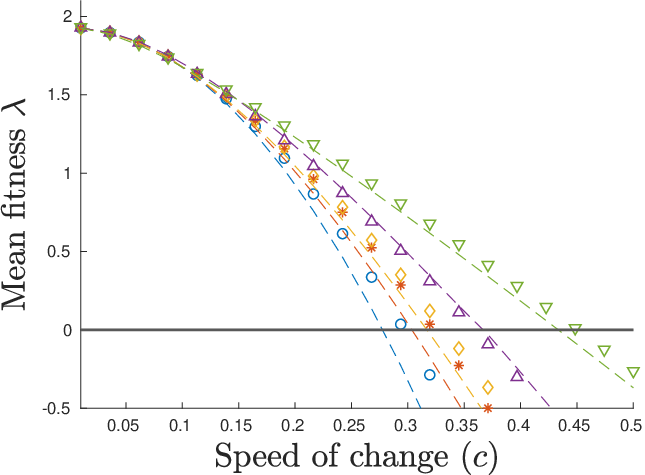
In addition, in the asexual model, this rate of increase will crucially depend on the shape of the mutation kernel through the Lagrangian function $L$. Indeed, we can show from our formula in Table 2 that the lag increases linearly with the speed of change $c$ as soon as the function $c\mapsto m^{-1}(L(c))$ is linear. Thus, both the shape of selection and that of the mutation kernel interact to determine how the evolutionary lag responds to faster environmental change. If the selection function is quadratic (i.e. $m(z)=z^{2}/2,$), we can show from the convexity of the Lagrangian function $L$ that the lag increases linearly with $c$ only in the diffusion approximation $L(c)=c^{2}/2$ (see Table 3 and blue curve in Fig. 2), while it increases sub–linearly for any other mutation kernels (see red, orange, purple and green curves in Fig. 2). We can further show that the lag in this scenario increases more slowly with the rate of environmental change when the kurtosis of the mutation kernel is higher (see Appendix D.4 for mathematical details). In Fig. 2, we compare four different mutation kernels with increasing kurtosis: uniform distribution kernel (red), Gaussian kernel (orange), double exponential kernel (purple) and Gamma kernel (green). In the asexual model, a fat tail of the mutation kernel thus tends to reduce the lag, even though this effect is most visible when the environment changes fast (Fig. 2) .

To examine the effect of the selection function on how the evolutionary lag increases in faster changing environment, we now focus on the case of diffusion approximation in the asexual model ($L(c)=c^{2}/2$), for the sake of simplicity, and compare it to the results in the infinitesimal model. In both cases, we can exhibit a simple criteria to decipher the nature of this increase. Let us first observe that, in those cases, the lag increases linearly with $c$ if the selection function is quadratic (see Table 3 and the blue curves in Fig. 3). The lag however accelerates with $c$ if $m$ is sub-quadratic in the following senses (see orange curves in Fig. 3):

Conversely, the lag decelerates with $c$ if $m$ is super-quadratic in the following senses (see red curves in Fig. 3):

The criteria are of different nature depending on the model of reproduction (asexual versus infinitesimal). However, they coincide in the case of a homogeneous selection function $m(z)=|z|^{p}$ $(p>1)$. Indeed, selection is super-quadratic in both cases if and only if $p>2$. More generally, the lag is reduced when the selection function has a stronger convexity in the sense of (4.2). This behavior is illustrated in Fig. 3.

As observed by  Osmond and Klausmeier 2017, we also find that the lag may diverge, i.e. grow infinite for some finite threshold in the speed of environmental change, when the selection function is too weak away from the optimum. Such ”evolutionary tipping point” are predicted, both for the infinitesimal model and in the asexual model, for some shapes of the selection function. The underlying mechanisms are however qualitatively different in the two models, as explained below.

In order to illustrate this phenomenon, we consider a bounded selection function depicted in Fig. 3 (orange curve). We find the following critical speed $\mathbf{c}^{*}_{tip}$,

so that the lag is finite if and only if $\mathbf{c}<\mathbf{c}^{*}_{tip}$, while the lag diverges if $\mathbf{c}>\mathbf{c}^{*}_{tip}$ and the population cannot keep pace with the environmental change. The difference between the two formulas can be understood through graphical arguments (see Fig. 4). In the asexual model, the lag at equilibrium is found where the mortality rate equals a specific value, which increases with the speed of change $\mathbf{c}$. This point is found where the selection function intersects an horizontal line, of higher elevation as $\mathbf{c}$ increases in Fig. 4. With a bounded mortality function, there is thus a finite value of $\mathbf{c}$ for which this critical quantity equals the maximal mortality rate, the latter being reached for an infinitely large lag. In the infinitesimal model, the equilibrium lag is found where the selection gradient equals a specific value increasing with $\mathbf{c}$. Graphically, this point is found where the local slope of the selection function equals such a critical value. With a bounded mortality function such as in Fig. 4, there are in general two equilibrium points characterized by such local slope, one stable in the convex part and one unstable in the concave part. As the speed of environmental change increases, so does the local slope at the two equilibria, which gradually converge towards the inflection point of the mortality function with the maximal local slope. This point characterizes the maximal speed of environmental change for which there is a finite evolutionary lag. Above that critical speed of change, the lag grows without limit. We illustrate this phenomenon of severe maladaptation in Fig. 3 (see the orange curves).

Despite the existence of tipping points in both cases, the transition from moderate ($\mathbf{c}<\mathbf{c}^{*}_{tip}$) to severe maladaptation ($\mathbf{c}>\mathbf{c}^{*}_{tip}$) have different signatures depending on the reproduction model. In the asexual model, the lag becomes arbitrarily large as the speed $\mathbf{c}$ becomes close to the maximal sustainable speed $\mathbf{c}^{*}_{tip}$. Conversely, in the infinitesimal model, the lag remains bounded by the value of the inflexion point until it drops to infinity when the speed becomes larger than $\mathbf{c}^{*}_{tip}$.

We can also see a major difference between the two reproduction models when we look at the time dynamics (Fig. 5). We run simulations of the density dynamics described by the equation (2.3) and starting from various initial data centered at different traits (see crosses in Fig. 5). In the infinitesimal model, when the initial lag is beyond the unstable point $z^{*}_{u}$, defined in Fig. 4(b), the lag diverges, whereas it converges to the stable point $z^{*}_{s}$, also defined in Fig. 4(b), if the lag is initially moderate. We see that the long term adaptation of the population to a changing environment does not only depend on the speed of change, but also on the initial state of the population. In the asexual model, the initial configuration of the population does not play a significant role in the long term dynamics of adaptation: we observe that the population can adapt whatever the initial lag is, if the speed of change is below $\mathbf{c}^{*}_{tip}$ (see Fig. 5). We can expect such difference because the lag at equilibrium is uniquely defined in the asexual model while it can take multiple values in the infinitesimal model if the function has an inflexion point, which is the case for the bounded selection function (see Fig 4).

In both scenarios the lag load $\triangle\boldsymbol{\lambda}$, defined as the difference between the mean fitness without changing environment ($\boldsymbol{\lambda}_{0}=\boldsymbol{\beta}-\boldsymbol{\mu}_{0}$) and the mean fitness under changing environment, is (unsurprisingly) given by the increment of mortality at the evolutionary lag $\mathbf{m}(\mathbf{z}_{0}^{*})$

Since $\mathbf{m}$ is symmetric increasing and the lag $|\mathbf{z}_{0}^{*}|$ is increasing with respect to $\mathbf{c}$, we deduce that the mean fitness decreases with respect to $\mathbf{c}.$ It is illustrated in Fig. 3 for different selection functions.

In the asexual model, the lag-load takes the following form

which is exactly the expression (3.4) in the original units with a speed $\mathbf{c}$. Since $L$ increases with the kurtosis of the mutation kernel, we deduce that higher kurtosis of the mutation kernel increases the mean fitness (see Fig. 2).

In the asexual model, the lag load only depends, at the leading order, on the speed of environmental change and the mutation kernel through the Lagrangian function $L$ (see Table 2). In particular, for a given speed $\mathbf{c}$, a fertility rate $\boldsymbol{\beta}$ and a given mutation kernel, we predict that the lag load is constant (see dashed line in Fig. 6(a)). At the next order of approximation, the mean fitness however depends on the local shape of the selection function around the optimal trait: $\boldsymbol{\alpha}=\mathbf{m}^{\prime\prime}(0)$. The mean fitness is then predicted to decline as the strength of stabilizing selection around the optimum $\boldsymbol{\alpha}$ increases (see Fig. 6(a)), due to increasing standing load.These predictions are confirmed by our numerical simulation see Fig. 3(a) and 6(a).

In contrast, the influence of the selection pattern is more intricate in the case of the infinitesimal model of reproduction. The lag load depends strongly on the global shape of $\mathbf{m}$ (see Fig. 3(b) and 6(b)). In particular, we see that for low strength of selection $\boldsymbol{\alpha}$, the mean fitness crucially depends on the shape of selection. Mean fitness is higher in the scenario with super–quadratic selection than with quadratic selection, and lowest when selection is sub-quadratic in Fig. 3(b) and 6(b)). Moreover, the mean fitness increases with increasing strength of selection in the quadratic case, while it initially decreases for the super–quadratic case. However, for stronger strength of selection, the shape of selection has less importance. Our approximation allows us to capture those differences. For instance, in the quadratic case (blue curves in Fig. 6 and 3), we can see from Table 3 that the mean fitness increases with the strength of selection $\boldsymbol{\alpha}$ at the leading order, which corresponds to small value of $\boldsymbol{\alpha}$. However, when the strength of selection becomes stronger, antagonistic effects occur at the next order so that the fitness may decrease due to standing load, defined in (3.5) (Lynch and Lande 1993; Lande and Shannon 1996; Kopp and Matuszewski 2014). This effect is illustrated in Fig. 6(b).

For the asexual model, we only compare the simulation results with our first order approximation stated in Table 2 (black colored), except for the variation of the mean fitness with respect to the strength of selection, where we need to take into account the standing load that appears at the second order of approximation (see gray colored formula in Table 2). We can first observe from Fig. 6 that our first approximations are accurate when $\varepsilon=\boldsymbol{\sigma}\sqrt{\boldsymbol{\alpha}/\boldsymbol{\beta}}$ is small (see value of $\boldsymbol{\alpha}<0.5$ in Fig. 6). The scale of Fig. 6(a) is of order $\varepsilon$, which is why the first order approximation seems less accurate than the second order approximation. This was expected since the standing load, which increases with the strength of selection, occurs at the second order of approximation. The approximation of $\mathbf{z}^{*}$ and $\boldsymbol{\lambda}$ remain efficient even when $\varepsilon$ increases (see Fig. 2 and 3 for small value of $\mathbf{c}$). However, we see that the approximations deviate from the simulations when the speed of change increases and reaches the critical value $\mathbf{c}^{*}$ (see Fig. 2 and 3) or when the mutation kernel becomes leptokurtic (see green curves of Fig. 2). The approximation of the standing variance is more sensitive to the parameter $\varepsilon$. When $\mathbf{c}$ and $\varepsilon$ are small it is accurate (see Fig. 2). However, when the speed increases, the approximation diverges from the simulations even if $\varepsilon$ is small (see Fig. 2 and 3).

For the infinitesimal model, we have compared our simulations to our first order approximation, as well as the second order approximation stated in Table 2 (first order approximation is black colored and second order approximation is gray colored). The first order approximation of $\mathbf{z}^{*}$ and $\boldsymbol{\lambda}$ are efficient only when $\varepsilon$ is really small, while the first order approximation of the standing variance may deviate from the simulation value even for small $\varepsilon$ (see red curve Fig. 6(f)). However, the second approximations are really precise for small value of $\varepsilon$ (see Fig. 6) and they remain efficient when $\varepsilon$ increases and $\mathbf{c}$ increases (see Fig. 6 and 3).

We compare the simulated equilibrium distribution $\mathbf{F}$ with our analytical approximations (Fig. 7): the first order approximation corresponds to $\mathbf{F}_{0}=\exp(-U_{0}/\varepsilon^{\gamma})$, where $U_{0}$ satisfies respectively the differential equation (3.1) (asexual model) or $U_{0}(z)=(z-z^{*}_{0})^{2}/2$ (infinitesimal sexual model), and $\gamma$ is respectively equal to $1$ in the asexual model and $2$ in the infinitesimal case; and the second order approximation $\mathbf{F}_{1}=\exp(-U_{0}/\varepsilon^{\gamma}-U_{1})$, where $U_{1}$ satisfies respectively equation (D.12) (asexual model) or the non–local functional equation (3.12) (infinitesimal model). Our simulations are performed with an $\varepsilon^{\gamma}=0.1$, which is not that small.

In the asexual model, we can observe that the first order analytical approximation is really efficient at tracking the shape of the entire distribution for both super-quadratic and quadratic selection, even if $\varepsilon$ is not that small (Fig. 7). For the bounded selection, our first order approximation fails to fit the left tail of the distribution, mainly because the speed of environmental change is close to the critical speed.

In the infinitesimal model, we can observe that the first order Gaussian approximation is not precise enough to track the entire distribution (Fig. 7). We need the second order approximation to fit the distribution. This is a direct consequence of our analysis, where we observe that we need the second order approximation to define the first order approximation of the lag $z^{*}_{0}$.

To go further in understanding the effect of a changing environment, we now look at the skewness and the kurtosis of the distributions. Those two indicators allow us to test whether the distribution $\mathbf{F}$ can be well approximated by the Gaussian distribution.

In the asexual model, we can observe from Fig. 8 that, even for the quadratic selection, the distributions differ from a Gaussian distribution: they are skewed and leptokurtic, which means that their kurtosis are higher than the kurtosis of the Gaussian distribution with same mean and variance. So the Gaussian distribution fails to track the exact distribution of the trait around the evolutionary lag of the population in a changing environment. This phenomenon is enhanced when the selection function differs from the quadratic function (see Fig. 8 diamond curves and  7). In addition, we see that, when the selection function is super–quadratic, the distribution has a positive skew, while, for a bounded selection function, it has a negative skew.

Conversely, in the infinitesimal case, the Gaussian distribution well approximates the equilibrium distribution in general. This was already described by our approximation formula (3.11) in the section 3.2. We can see that the kurtosis of the equilibrium distribution remains close to zero for any speeds of change and any selection functions.However, when the selection function is either super quadratic or bounded, we can observe from Fig. 7 and 8 that the distribution of phenotypes in the infinitesimal model also becomes skewed as the speed increases. The skew of the distribution corresponds to regions where the gradient of selection is low, with the same pattern as in the asexual model.

References

- Alexander et al. [2014] H K Alexander, G Martin, O Y Martin, and S Bonhoeffer. Evolutionary rescue: linking theory for conservation and medicine. Evolutionary applications, 7(10):1161–1179, 2014.
- Barton and Keightley [2002] N. H. Barton and P. D. Keightley. Understanding quantitative genetic variation. Nature Reviews Genetics, 3(1):11–21, 2002. doi: 10.1038/nrg700.
- Barton and Turelli [1987] N H Barton and M Turelli. Adaptive landscapes, genetic distance and the evolution of quantitative characters. Genetical Research, 49(2):157–173, 1987. doi: 10.1017/S0016672300026951.
- Barton and Turelli [1989] N. H. Barton and M Turelli. Evolutionary quantitative genetics: how little do we know? Annual Review of Genetics, 23(1):337–370, 1989. doi: 10.1146/annurev.ge.23.120189.002005.
- Barton et al. [2017] N H Barton, A M Etheridge, and A Véber. The infinitesimal model. Theoretical Population Biology, 118:50–73, 2017. doi: 10.1101/039768.
- Bulmer [1971] M G Bulmer. The effect of selection on genetic variability. Amer. Nat., 105(943):201–211, 1971.
- Bulmer [1974] M. G. Bulmer. Linkage disequilibrium and genetic variability. Genet. Res., 23:281–289, 1974.
- Bulmer [1980] M G Bulmer. The Mathematical Theory of Quantitative Genetics. Oxford, Clarendon Press, 1980.
- Burger [1991] R Burger. Moments, cumulants, and polygenic dynamics. J. Math. Biol., 30(2):199–213, 1991.
- Bürger [2000] R. Bürger. The Mathematical Theory of Selection, Recombination, and Mutation. Wiley Series in Mathematical & Computational Biology. Wiley, 2000. ISBN 9780471986539.
- Burger and Lynch [1995] R Burger and M Lynch. Evolution and Extinction in a Changing Environment: A Quantitative-Genetic Analysis. Evolution, 49(1):151–163, 1995. doi: 10.2307/2410301.
- Bürger [1999] R Bürger. Evolution of Genetic Variability and the Advantage of Sex and Recombination in Changing Environments. Genetics, 153(2):1055–1069, 1999. doi: 10.1093/genetics/153.2.1055.
- Calvez and Lam [2020] V Calvez and K Y Lam. Uniqueness of the viscosity solution of a constrained hamilton–jacobi equation. Calc. Var., 59(163), 2020. doi: 10.1007/s00526-020-01819-0.
- Calvez et al. [2018] V Calvez, C Henderson, S Mirrahimi, O Turanova, and T Dumont. Non-local competition slows down front acceleration during dispersal evolution, 2018.
- Calvez et al. [2019] V Calvez, J Garnier, and F Patout. Asymptotic analysis of a quantitative genetics model with nonlinear integral operator. J École polytechnique — Mathématiques, 6:537–579, 2019. doi: 10.5802/jep.100.
- Calvez et al. [2021] V Calvez, B Henry, S Méléard, and V Chi Tran. Dynamics of lineages in adaptation to a gradual environmental change, 2021.
- Charlesworth [1993] B Charlesworth. Directional selection and the evolution of sex and recombination. Genetical Research, 61(3):205–224, 1993. doi: 10.1017/S0016672300031372.
- Cloez and Gabriel [2020] B Cloez and P Gabriel. On an irreducibility type condition for the ergodicity of nonconservative semigroups. Comptes Rendus. Mathématique, 358(6):733–742, 2020.
- Cotto and Ronce [2014] O Cotto and O Ronce. Maladaptation as a source of senescence in habitats variable in space and time. Evolution, 68(1):2481–2493, 2014. doi: 10.1111/evo.12462.
- Coville and Hamel [2019] J Coville and F Hamel. On generalized principal eigenvalues of nonlocal operators witha drift. Nonlinear Analysis, page 111569, 2019.
- Dekens [2020] L Dekens. Evolutionary dynamics of complex traits in sexual populations in a strongly heterogeneous environment: how normal?, 2020.
- Dekens and Lavigne [2021] L Dekens and F Lavigne. Front propagation of a sexual population with evolution of dispersion: a formal analysis, 2021.
- Dekens and Mirrahimi [2021] L Dekens and S Mirrahimi. Dynamics of dirac concentrations in the evolution of quantitative alleles with sexual reproduction, 2021.
- Dekens et al. [2021] L Dekens, S P Otto, and V Calvez. The best of both worlds: combining population genetic and quantitative genetic models, 2021.
- Diekmann et al. [2005] O Diekmann, P-E Jabin, S Mischler, and B Perthame. The dynamics of adaptation: An illuminating example and a hamilton–jacobi approach. Theoretical Population Biology, 67(4):257 – 271, 2005. doi: http://dx.doi.org/10.1016/j.tpb.2004.12.003.
- Dimassi and Sjostrand [1999] M Dimassi and J Sjostrand. Spectral Asymptotics in the Semi-Classical Limit. London Mathematical Society Lecture Note Series. Cambridge University Press, 1999. ISBN 9780521665445.
- Evans [2010] L C. Evans. Partial differential equations. American Mathematical Society, Providence, R.I., 2010. ISBN 9780821849743 0821849743.
- Evans and Ishii [1985] L C Evans and H Ishii. A PDE approach to some asymptotic problems concerning random differential equations with small noise intensities. Ann. Inst. H. Poincaré Anal. Non Linéaire, 2(1):1–20, 1985.
- Fisher [1918] R A Fisher. The correlation between relatives on the supposition of Mendelian inheritance. Trans. R. Soc. Edinburgh, 52:399–433, 1918.
- Fleming [1977] W H. Fleming. Exit probabilities and optimal stochastic control. Appl. Math. Optim., 4(1):329–346, 1977. doi: 10.1007/BF01442148.
- Fleming [1979] W H Fleming. Equilibrium distributions of continuous polygenic traits. SIAM J. Appl. Math., 36(1):148–168, 1979. doi: 10.1137/0136014.
- Frank and Slatkin [1990] S A Frank and M Slatkin. The distribution of allelic effects under mutation and selection. Genetical Research, 55(2):111–117, 1990. doi: 10.1017/S0016672300025350.
- Friedlin and Wentzell [2012] M I Friedlin and A D Wentzell. Random perturbations of dynamical systems. Springer, 2012.
- Gauzere et al. [2020] J Gauzere, B Teuf, H Davi, L-M Chevin, T Caignard, B Leys, S Delzon, O Ronce, and I Chuine. Where is the optimum? predicting the variation of selection along climatic gradients and the adaptive value of plasticity. a case study on tree phenology. Evolution letters, 4(2):109—123, 2020. doi: 10.1002/evl3.160.
- Halligan and Keightley [2009] D. L. Halligan and P. D. Keightley. Spontaneous mutation accumulation studies in evolutionary genetics. Annual Review of Ecology, Evolution, and Systematics, 40(1):151–172, 2009. doi: 10.1146/annurev.ecolsys.39.110707.173437.
- Hill [2010] W. G. Hill. Understanding and using quantitative genetic variation. Philosophical Transactions of the Royal Society B: Biological Sciences, 365(1537):73–85, 2010. doi: 10.1098/rstb.2009.0203.
- Johnson and Barton [2005] T. Johnson and N. Barton. Theoretical models of selection and mutation on quantitative traits. Philosophical Transactions of the Royal Society B: Biological Sciences, 360(1459):1411–1425, 2005. doi: 10.1098/rstb.2005.1667.
- Jones et al. [2012] A. G. Jones, R. Bürger, S. J. Arnold, P. A. Hohenlohe, and J. C. Uyeda. The effects of stochastic and episodic movement of the optimum on the evolution of the g-matrix and the response of the trait mean to selection. J. Evol. Biol., 25(11):2210–2231, 2012. doi: https://doi.org/10.1111/j.1420-9101.2012.02598.x.
- Keightley and Hill [1988] P. D. Keightley and W. G. Hill. Quantitative genetic variability maintained by mutation-stabilizing selection balance in finite populations. Genet. Res., 52:33–43, 1988.
- Kimura [1965] M Kimura. A stochastic model concerning the maintenance of genetic variability in quantitative characters. Proc. Natl. Acad. Sci. USA, 54(3):731–736, 1965. doi: 10.1073/pnas.54.3.731.
- Klausmeier et al. [2020] Christopher A. Klausmeier, Matthew M. Osmond, Colin T. Kremer, and Elena Litchman. Ecological limits to evolutionary rescue. Philosophical Transactions of the Royal Society B: Biological Sciences, 375(1814):20190453, 2020. doi: 10.1098/rstb.2019.0453.
- Kopp and Matuszewski [2014] Michael Kopp and Sebastian Matuszewski. Rapid evolution of quantitative traits: theoretical perspectives. Evolutionary Applications, 7(1):169–191, 2014.
- Lam [2017] K Y Lam. Stability of dirac concentrations in an integro-pde model for evolution of dispersal. Calc. Var., 59(79), 2017. doi: 10.1007/s00526-017-1157-1.
- Lam and Lou [2017] K Y Lam and Y Lou. An integro-pde model for evolution of random dispersal. J. Func. Anal., 272(5):1755–1790, 2017. ISSN 0022-1236. doi: 10.1016/j.jfa.2016.11.017.
- Lande [1975] R Lande. The maintenance of genetic variability by mutation in a polygenic character with linked loci. Genetical Research, 26(3):221–235, 1975. doi: 10.1017/S0016672300016037.
- Lande and Shannon [1996] R Lande and S Shannon. The role of genetic variation in adaptation and population persistence in a changing environment. Evolution, 50(1):434–437, 1996. doi: 10.2307/2410812.
- Lange [1978] K J Lange. Central limit theorems of pedigrees. J. Math. Biol., 6(1):59–66, 1978.
- Lorz et al. [2011] A Lorz, S Mirrahimi, and B Perthame. Dirac mass dynamics in multidimensional nonlocal parabolic equations. Commun. Partial Differential Equations, 36(6):1071–1098, 2011.
- Lynch and Lande [1993] M Lynch and R Lande. Evolution and extinction in response to environmental change. Sinauer Assoc. 1993.
- Lynch et al. [1991] M. Lynch, W. Gabriel, and A. M. Wood. Adaptive and demographic responses of plankton populations to environmental change. Limnology and Oceanography, 36:1301–1312, 1991.
- Martin and Roques [2016] G Martin and L Roques. The non-stationary dynamics of fitness distributions: Asexual model with epistasis and standing variation. Genetics, 204:1541–1558, 2016. doi: 10.1534/genetics.116.187385.
- Mirrahimi [2017] S Mirrahimi. A hamilton–jacobi approach to characterize the evolutionary equilibria in heterogeneous environments. Mathematical Models and Methods in Applied Sciences, 27(13):2425–2460, 2017. doi: 10.1142/S0218202517500488.
- Mirrahimi and Raoul [2013] S Mirrahimi and G Raoul. Population structured by a space variable and a phenotypical trait. Theor. Popul. Biol., 84:87–103, 2013.
- Mirrahimi and Roquejoffre [2016] S Mirrahimi and J-M Roquejoffre. A class of hamilton–jacobi equations with constraint: Uniqueness and constructive approach. J. Diff. Equ., 260(5):4717–4738, 2016. doi: https://doi.org/10.1016/j.jde.2015.11.027.
- Nei [2014] M. Nei. Mutation-Driven Evolution. Oxford University Press, 2014. ISBN 9780198724100.
- Osmond and Klausmeier [2017] M M Osmond and C A Klausmeier. An evolutionary tipping point in a changing environment. Evolution, 71(12):2930–2941, 2017. doi: 10.1111/evo.13374.
- Patout [2019] F Patout. Analyse asymptotique d’équations intégro-différentielles : modèles d’évolution et de dynamique des populations. Theses, Université de Lyon, 2019.
- Patout [2020] F Patout. The cauchy problem for the infinitesimal model in the regime of small variance. arXiv:2001.04682, 2020.
- Patout et al. [2020] F Patout, R Forien, and J Garnier. Ancestral lineages in mutation-selection equilibria with moving optimum, 2020.
- Perthame [2007] B Perthame. Transport equations in biology. Frontiers in Mathematics. Birkhäuser Verlag, 2007.
- Perthame and Barles [2008] B Perthame and G Barles. Dirac concentrations in Lotka-Volterra parabloci PDEs. Indiana Univ. Math. J., 457(7):3275–3301, 2008.
- Perthame and Souganidis [2016] B Perthame and P E Souganidis. Rare mutations limit of a steady state dispersal evolution model. Math. Model. Nat. Phenom., 11(4):154–166, 2016. doi: 10.1051/mmnp/201611411.
- Raoul [2021] G Raoul. Exponential convergence to a steady-state for a population genetics model with sexual reproduction and selection, 2021.
- Rauch [2012] J Rauch. Hyperbolic partial differential equations and geometric optics, volume 133. American Mathematical Society Providence, RI, 2012.
- Rockafellar [1970] R T Rockafellar. Convex Analysis. Princeton landmarks in mathematics and physics. Princeton University Press, 1970. ISBN 9780691015866.
- Roques et al. [2020] L Roques, F Patout, O Bonnefon, and G Martin. Adaptation in general temporally changing environments. SIAM J. Appl. Math., 80(6):2420–2447, 2020. doi: 10.1137/20M1322893.
- Santiago [1998] E Santiago. Linkage and the maintenance of variation for quantitative traits by mutation–selection balance: an infinitesimal model. Genet Res, 71(2):161–170, 1998. doi: 10.1017/S0016672398003231.
- Tufto [2000] J Tufto. Quantitative genetic models for the balance between migration and stabilizing selection. Genetical research, 76(03):285–293, 2000.
- Turelli [1984] M Turelli. Heritable genetic variation via mutation-selection balance: Lerch’s zeta meets the abdominal bristle. Theor. Popul. Biol., 25(2):138–193, 1984. doi: 10.1016/0040-5809(84)90017-0.
- Turelli [2017] M Turelli. Commentary: Fisher’s infinitesimal model: A story for the ages. Theoretical Population Biology, 118:46 – 49, 2017. doi: https://doi.org/10.1016/j.tpb.2017.09.003.
- Turelli and Barton [1990] M Turelli and N H Barton. Dynamics of polygenic characters under selection. Theor. Popul. Biol., 38(1):1–57, 1990. doi: https://doi.org/10.1016/0040-5809(90)90002-D.
- Turelli and Barton [1994] M Turelli and N H Barton. Genetic and statistical analyses of strong selection on polygenic traits: what, me normal? Genetics, 138(3):913–941, 1994.
- W Hao [2021] Y Lou W Hao, K-Y Lam. Ecological and evolutionary dynamics in advective environments: Critical domain size and boundary conditions. Disc. Conti. Dyn. Syst. - B, 26(1):367–400, 2021.
- Walters et al. [2012] R J Walters, W U Blanckenhorn, and D Berger. Forecasting extinction risk of ectotherms under climate warming: an evolutionary perspective. Functional Ecology, 26(6):1324–1338, 2012.
- Waxman and Peck [1999] D Waxman and J R Peck. Sex and Adaptation in a Changing Environment. Genetics, 153(2):1041–1053, 1999. doi: 10.1093/genetics/153.2.1041.
- Zworski [2012] M Zworski. Semiclassical analysis, volume 138. American Mathematical Society Providence, RI, 2012.
Supplementary material/Appendix
The following subsections gather mathematical analysis supporting the adimensional scaling, numerical methods, Taylor expansions and formula derived in the main text. Although some parts are standard methods (rescaling, numerics), some parts are original contributions (dedicated Taylor expansions and formula involving the Lagrangian function), extending the literature in multiple ways. Hence, this supplementary material can be read as the companion mathematical paper of the main text.
Before we enter into the technical details, let us highlight some important observations about the Taylor expansions:
- •
These expansions are more than moment closure methods, where one usually tries to guess the higher moments of the distribution in order to derive a close system of equations on some scalar quantities (first moments of the distribution, e.g. population size, evolutionary lag value, etc). Here, the whole distribution is approximated, then scalar quantities are deduced without any a priori assumptions on the shape of the distribution.
In contrast to classical expansions of the distribution which are linear, e.g. , we perform here a multiplicative Taylor expansion, meaning a linear expansion of the logarithm of the density: . We claim this is the natural expansion in the regime of small variance in order to discard the variance from the asymptotic calculations. Nonetheless, intermediate computations may appear heavy because of the nonlinear nature of the multiplicative expansion.
We believe all these approximations can be theoretically justified, and error terms can be controlled quantitatively up to some extent. Results in the literature so far cover the case without environmental change (c = 0), see [Perthame and Barles 2008, Mirrahimi and Raoul 2013] (Barles, Perthame, Mirrahimi et al) for the asexual model, and the more recent [Calvez et al. 2019, Patout 2020] for the infinitesimal sexual model.
Appendix A Derivation of generic formula
Let us consider the equilibrium of our model: