跳到论文正文
W Papers独立论文阅读器 arXiv:2206.13200 论文正文 计算阅读时间 · 0%
引用这篇论文根据当前论文元数据生成,正式投稿前建议核对。


License: CC BY-NC-ND 4.0
arXiv:2206.13200v1 [math.PR] 27 Jun 2022

Bivariate compound Poisson risk processes with shocks
(Working version)
Pavlina K. Jordanova
Faculty of Mathematics and Informatics, Konstantin Preslavsky University of Shumen,
115 ”Universitetska” str., 9712 Shumen, Bulgaria.
Corresponding author: pavlina_kj@abv.bg

Evelina Veleva
Department of Applied mathematics and Statistics, ”Angel Kanchev” University of Ruse, Bulgaria.
Kosto Mitov
Department of Medical Physics, Biophysics, Pre-clinical and Clinical Sciences, Medical University - Pleven, Bulgaria.

Abstract

Contemporary insurance theory is concentrated on models with different types of polices and shock events may influence the payments on some of them. Jordanova [7] considered a model where a shock event contributes to the total claim amount with one and the same value of the claim sizes to different types of polices. Jordanova and Veleva [8] went a step closer to real life situations and allowed a shock event to cause different claim sizes to different types of polices. In that paper the counting process is assumed to be Multinomial. Here it is replaced with different independent homogeneous Poison processes. The bivariate claim counting process is expressed in two different ways. Its marginals and conditional distributions are totaly described. The mean square regression of these processes is computed. The Laplace-Stieltjes transforms and numerical characteristics of the total claim amount processes are obtained. The risk reserve process and the probabilities of ruin in infinite time are discussed. The risk reserve just before the ruin and the deficit (or the severity) at ruin are thoroughly investigated in case when the initial capital is zero. Their means, probability mass functions and probability generating functions are obtained.

Although the model is constructed by a multivariate counting processes, along the paper it is shown that the total claim amount process is stochastically equivalent to a univariate compound Poisson process. These allows us to reduce the considered risk model to a Cramer-Lundberg risk model, to use the corresponding results and to make the conclusions for the new model. Analogous results can be obtained for more types of polices and more types of shock events.

The results are applied in case when the claim sizes are exponentially distributed.

Stochastically equivalent models could be analogously constructed in queuing theory.

1 DESCRIPTION OF THE MODEL AND ITS RELATIONS WITH PREVIOUSLY INVESTIGATED MODELS

The origin of modeling of random processes with common shocks is usually related with the names of Marshal and Olkin [14, 15] or Mardia [13]. They construct different bivariate models with dependent coordinates, where the dependence is caused by a joint summand, or a joint term in the maxima or the minima. The results could be easily transferred to random processes with independent increments. Cossette and Marceau [3] apply such results in risk theory. Jordanova [7] uses merging of compound Poisson processes and investigates a particular case of the model, defined in this work. The difference is that, in that work, in a fixed point of time, if there is a shock event it affects different types of contracts via one and the same claim size. In the insurance model investigated in Jordanova and Veleva [8] the form of the dependence is improved. The claim sizes caused by one and the same shock event on different types of polices can be different. However, in that paper, the counting processes of claim arrivals of different types of polices are described via a Multinomial processes. Here this Multinomial process is replaced with different independent homogeneous Poisson processes (HPPs) and the form of the dependence is the same. More precisely, let N0N_{0}, N1N_{1}, N2N_{2} be mutually independent HPPs with parameters correspondingly λ0>0\lambda_{0}>0, λ1>0\lambda_{1}>0 and λ2>0\lambda_{2}>0. By assumption N0​(0)=N1​(0)=N2​(0)=0N_{0}(0)=N_{1}(0)=N_{2}(0)=0.

The counting processes M1M_{1} and M2M_{2} of both types of claims are in generally dependent HPP with common shocks, and for all t≥0t\geq 0

M1​(t)=N1​(t)+N0​(t),M2​(t)=N2​(t)+N0​(t),M_{1}(t)=N_{1}(t)+N_{0}(t),\quad M_{2}(t)=N_{2}(t)+N_{0}(t), (1)

Therefore, M1M_{1} is a HPP with parameter λ1+λ0\lambda_{1}+\lambda_{0} and M2M_{2} is a HPP with parameter λ2+λ0\lambda_{2}+\lambda_{0}.

The total claim amount process S={S⁡(t):t≥0}S=\{S(t):t\geq 0\} is such that for all t≥0t\geq 0,

S⁡(t)\displaystyle S(t) =\displaystyle= S1​(t)+S2​(t),\displaystyle S_{1}(t)+S_{2}(t), (2)
S1​(t)\displaystyle S_{1}(t) =\displaystyle= ∑i=0N1​(t)Y1​i+∑i=0N0​(t)Y3​i,Y10=0,Y30=0\displaystyle\sum_{i=0}^{N_{1}(t)}Y_{1i}+\sum_{i=0}^{N_{0}(t)}Y_{3i},\quad Y_{10}=0,\,\,Y_{30}=0 (3)
S2​(t)\displaystyle S_{2}(t) =\displaystyle= ∑i=0N2​(t)Y2​i+∑i=0N0​(t)Y4​i,Y20=0,Y40=0.\displaystyle\sum_{i=0}^{N_{2}(t)}Y_{2i}+\sum_{i=0}^{N_{0}(t)}Y_{4i},\quad Y_{20}=0,\,\,Y_{40}=0.

The sequences {Yk​i}i=1∞\{Y_{ki}\}_{i=1}^{\infty} and {Nr​(s),s≥0}\{N_{r}(s),s\geq 0\}, k=1,2,3,4k=1,2,3,4, r=0,1,2r=0,1,2 are mutually independent. The processes S1={S1​(t),t≥0}S_{1}=\{S_{1}(t),\,t\geq 0\} and S2={S2​(t),t≥0}S_{2}=\{S_{2}(t),\,t\geq 0\} are in generally dependent.

The definitions of SS, S1S_{1} and S2S_{2} mean that we allow the claims to be of two mutually exclusive different types and shock events (like car-crashes) may cause possibly different payments in both polices. The process N0={N0​(t),t≥0}N_{0}=\{N_{0}(t),\,t\geq 0\} describes the counts of shock events. In (3) for any fixed k=1,2,3,4k=1,2,3,4 the random variables (r.vs.) Yk​1,Yk​2,…Y_{k1},Y_{k2},... are independent identically distributed (i.i.d.) with cumulative distribution function (c.d.f.) 𝔽k\mathbb{F}_{k}. The sequences {Y1​i}i=1∞\{Y_{1i}\}_{i=1}^{\infty}, {Y2​i}i=1∞\{Y_{2i}\}_{i=1}^{\infty} and {(Y3​i,Y4​i)}i=1∞\{(Y_{3i},Y_{4i})\}_{i=1}^{\infty} are mutually independent. Without lost of generality the almost sure strictly positive r.v. Yk​iY_{ki} describes the ii-th claim amount, (i∈ℕi\in\mathbb{N}) of a certain type kk, k∈{1,2,3,4}k\in\{1,2,3,4\}. If the distribution of the claim sizes has mass at zero, the parameters of the corresponding counting HPPs, participating in S1S_{1} and S2S_{2}, defined in (3), can be changed, and the model can be reduced to the considered here one.

A natural example of an insurance interpretation of this model is as follows. For k=1k=1, Y1​iY_{1i} is the part of the claim size which is due to the customer for ii-th standard insurance policy of type 11 exclusively the common shocks. Analogously for k=2k=2. The r.v. Y3​i+Y4​iY_{3i}+Y_{4i} models the part of the claim size which have to be paid to the customer due to some common shock. Jordanova and Veleva [8] give and example when the random elements with k=1k=1 describe health insurances, k=2k=2 is for car insurance. Then, ∑i=0N1​(t)Y1​i\sum_{i=0}^{N_{1}(t)}Y_{1i} is the total claim amount up to time tt, which is due to customers for having some healthy problems, not related with car-crashes. The r.v. ∑i=0N0​(t)Y3​i\sum_{i=0}^{N_{0}(t)}Y_{3i} models the total claim amount up to time tt, which is due to healthy problems, caused by car-crashes. The r.v. ∑i=0N2​(t)Y2​i\sum_{i=0}^{N_{2}(t)}Y_{2i} is for the total claim amount up to time tt, which is due to some car problems which are not related with car-crashes, for example car-thefts. And finally, the r.v. ∑i=1N0​(t)Y4​i\sum_{i=1}^{N_{0}(t)}Y_{4i} is the total claim amount up to time tt, which is due to some car problems which are related with car-crashes. Therefore, the random process S1S_{1} is the total claim amount processes for the insurance events caused by ”healthy problems”, S2S_{2} is the amount paid to customers for events caused by ”problems with cars”.

As usually the risk reserve process Ru={Ru​(t):t≥0}R_{u}=\{R_{u}(t):t\geq 0\} is defined via the equality

Ru​(t)=u+c​t−S⁡(t),t≥0,R_{u}(t)=u+ct-S(t),\quad t\geq 0, (4)

where u≥0u\geq 0 is the initial capital and c>0c>0 is the premium income rate per unit time.

The time of ruin when the initial capital is uu will be denoted by

τ⁡(u)\displaystyle\tau(u) :⁣=\displaystyle:= inf{t>0:Ru​(t)<0},inf∅=∞,\displaystyle\inf\{t>0:R_{u}(t)<0\},\quad\inf\,\emptyset=\infty, (5)

The probability for ruin in ”infinite horizon” and initial capital uu is

ψ⁡(u):=ℙ⁡(τ⁡(u)<∞).\psi(u):=\mathbb{P}(\tau(u)<\infty). (6)

and the corresponding survival probability is δ⁡(u):=1−ψ⁡(u)\delta(u):=1-\psi(u).

All random elements discussed here are assumed to be measurable with respect to one the same probability space (Ω,ℱ,ℙ)(\Omega,\mathcal{F},\mathbb{P}) with natural filtration born by the considered processes. The letter 𝔾\mathbb{G} is a notation for probability generating function (p.g.f.). Analogously, the letter 𝕃\mathbb{L} means Laplace-Stieltjes transform (LST).

2 THE BIVARIATE COUNTING PROCESS

Poisson and compound Poisson processes are very well investigated in the scientific literature. See for example Kingman [9], or Sundt and Vernic [17]. In multivariate case we have two types of compound Poisson processes. The I type means ”with equal number of summands”. The type ”II” is its opposite. Let us now derive the compound Poisson presentation of the first type of the bivariate counting process (M1,M2):={(M1​(t),M2​(t)):t≥0}(M_{1},M_{2}):=\{(M_{1}(t),M_{2}(t)):t\geq 0\}, defined in (1). In order to formulate our results we will define a random vector (I1,I2,I0)(I_{1},I_{2},I_{0}) with probability mass function (p.m.f.)

ℙ⁡(I1=1,I2=0,I0=0)=λ1λ,ℙ⁡(I1=0,I2=1,I0=0)=λ2λ,ℙ⁡(I1=0,I2=0,I0=1)=λ0λ,\mathbb{P}(I_{1}=1,I_{2}=0,I_{0}=0)=\frac{\lambda_{1}}{\lambda},\,\,\mathbb{P}(I_{1}=0,I_{2}=1,I_{0}=0)=\frac{\lambda_{2}}{\lambda},\,\,\mathbb{P}(I_{1}=0,I_{2}=0,I_{0}=1)=\frac{\lambda_{0}}{\lambda}, (7)

and zero otherwise. Here λ0>0\lambda_{0}>0, λ1>0\lambda_{1}>0, λ2>0\lambda_{2}>0 and λ:=λ0+λ1+λ2\lambda:=\lambda_{0}+\lambda_{1}+\lambda_{2}. By assumption the random vectors (I11,I21,I01),(I12,I22,I02),…(I_{11},I_{21},I_{01}),(I_{12},I_{22},I_{02}),... are i.i.d. with p.m.f. (7).

Denote by, N={N⁡(t),t≥0}N=\{N(t),\,t\geq 0\} a HPP with N⁡(0)=0N(0)=0, and parameter λ\lambda, and by

A1​(t):=∑i=0N⁡(t)(I1​i+I0​i),A2​(t):=∑i=0N⁡(t)(I2​i+I0​i),t≥0.A_{1}(t):=\sum_{i=0}^{N(t)}(I_{1i}+I_{0i}),\quad A_{2}(t):=\sum_{i=0}^{N(t)}(I_{2i}+I_{0i}),\quad t\geq 0. (8)

Here I10=I20=I00=0I_{10}=I_{20}=I_{00}=0 and NN and (I11,I21,I01),(I12,I22,I02),…(I_{11},I_{21},I_{01}),(I_{12},I_{22},I_{02}),... are independent. In our example the random process A1A_{1} counts the number of the insurance events caused by healthy problems. The random process A2A_{2} counts the number of the insurance events caused by problems with cars.

In the next theorem we show that the bivariate counting process (M1,M2):={(M1​(t),M2​(t)):t≥0}(M_{1},M_{2}):=\{(M_{1}(t),M_{2}(t)):t\geq 0\} is a particular case of a multivariate homogeneous in time compound Poisson process with equal number of summands, i.e. of type I, in the sense of Sundt and Vernic [17, 18].

Theorem 1. The bivariate counting processes (M1,M2)(M_{1},M_{2}) and (A1,A2)(A_{1},A_{2}) coincide in the sense of their finite dimensional distributions.

Proof: The processes (M1,M2)(M_{1},M_{2}) and (A1,A2)(A_{1},A_{2}) have homogeneous and independent additive increments and they start from the coordinate beginning. Therefore, in order to prove their stochastic equivalence it is enough to prove equality of their univariate time intersections. Due to the uniqueness of the correspondence between the probability laws and their p.g.fs. it is enough to derive equality between the p.g.fs.

The definition of p.g.fs., (1), the multiplicative property of p.g.f. and the well-known formula for the p.g.f. of the Poisson distribution entail that for all t≥0t\geq 0,

𝔼\displaystyle\mathbb{E} [z1M1​(t)​z2M2​(t)]=𝔼⁡[z1N1​(t)+N0​(t)​z2N2​(t)+N0​(t)]=𝔼⁡[z1N1​(t)​z2N2​(t)​(z1​z2)N0​(t)]=𝔼⁡[z1N1​(t)]​𝔼​[z2N2​(t)]​𝔼​[(z1​z2)N0​(t)]\displaystyle\left[z_{1}^{M_{1}(t)}z_{2}^{M_{2}(t)}\right]=\mathbb{E}\left[z_{1}^{N_{1}(t)+N_{0}(t)}z_{2}^{N_{2}(t)+N_{0}(t)}\right]=\mathbb{E}\left[z_{1}^{N_{1}(t)}z_{2}^{N_{2}(t)}(z_{1}z_{2})^{N_{0}(t)}\right]=\mathbb{E}\left[z_{1}^{N_{1}(t)}\right]\mathbb{E}\left[z_{2}^{N_{2}(t)}\right]\mathbb{E}\left[(z_{1}z_{2})^{N_{0}(t)}\right]
=\displaystyle= exp⁡{−λ1​t​(1−z1)}​exp⁡{−λ2​t​(1−z2)}​exp​{−λ0​t​(1−z1​z2)}=exp⁡(−λ​t+λ1​t​z1+λ2​t​z2+λ0​t​z1​z2).\displaystyle\exp\{-\lambda_{1}t(1-z_{1})\}\exp\{-\lambda_{2}t(1-z_{2})\}\exp\{-\lambda_{0}t(1-z_{1}z_{2})\}=\exp(-\lambda t+\lambda_{1}tz_{1}+\lambda_{2}tz_{2}+\lambda_{0}tz_{1}z_{2}).

By the definition (30), the formula for double expectations and the definition of Poisson distribution

𝔼⁡[z1A1​(t)​z2A2​(t)]\displaystyle\mathbb{E}\left[z_{1}^{A_{1}(t)}z_{2}^{A_{2}(t)}\right] =\displaystyle= 𝔼⁡[z1∑i=0N⁡(t)(I1​i+I0​i)​z2∑i=0N⁡(t)(I2​i+I0​i)]=∑n=0∞𝔼⁡[z1∑i=0n(I1​i+I0​i)​z2∑i=0n(I2​i+I0​i)]​ℙ​(N⁡(t)=n)\displaystyle\mathbb{E}\left[z_{1}^{\sum_{i=0}^{N(t)}(I_{1i}+I_{0i})}z_{2}^{\sum_{i=0}^{N(t)}(I_{2i}+I_{0i})}\right]=\sum_{n=0}^{\infty}\mathbb{E}\left[z_{1}^{\sum_{i=0}^{n}(I_{1i}+I_{0i})}z_{2}^{\sum_{i=0}^{n}(I_{2i}+I_{0i})}\right]\mathbb{P}(N(t)=n)
=\displaystyle= ∑n=0∞𝔼⁡[z1∑i=0n(I1​i+I0​i)​z2∑i=0n(I2​i+I0​i)]​(λ​t)nn!​e−λ​t.\displaystyle\sum_{n=0}^{\infty}\mathbb{E}\left[z_{1}^{\sum_{i=0}^{n}(I_{1i}+I_{0i})}z_{2}^{\sum_{i=0}^{n}(I_{2i}+I_{0i})}\right]\frac{(\lambda t)^{n}}{n!}e^{-\lambda t}.

By the multiplicative property of p.g.fs. and the fact that the random vectors (I11,I21,I01),(I12,I22,I02),…(I_{11},I_{21},I_{01}),(I_{12},I_{22},I_{02}),... are i.i.d. we have

𝔼⁡[z1A1​(t)​z2A2​(t)]=∑n=0∞[𝔼⁡(z1I11+I01​z2I21+I01)]n​(λ​t)nn!​e−λ​t.\mathbb{E}\left[z_{1}^{A_{1}(t)}z_{2}^{A_{2}(t)}\right]=\sum_{n=0}^{\infty}\left[\mathbb{E}\left(z_{1}^{I_{11}+I_{01}}z_{2}^{I_{21}+I_{01}}\right)\right]^{n}\frac{(\lambda t)^{n}}{n!}e^{-\lambda t}. (9)

Now, by using (7) we obtain the p.g.f. of 𝔼⁡[z1I11+I01​z2I21+I01]\mathbb{E}\left[z_{1}^{I_{11}+I_{01}}z_{2}^{I_{21}+I_{01}}\right]. Therefore, the fact that NN is a HPP with parameter λ\lambda and the Maclaurin series leads us to

𝔼⁡[z1A1​(t)​z2A2​(t)]\displaystyle\mathbb{E}\left[z_{1}^{A_{1}(t)}z_{2}^{A_{2}(t)}\right] =\displaystyle= ∑n=0∞[λ1λ​z1+λ2λ​z2+λ0λ​z1​z2]n​(λ​t)nn!​e−λ​t=exp⁡(−λ​t+λ1​t​z1+λ2​t​z2+λ0​t​z1​z2).\displaystyle\sum_{n=0}^{\infty}\left[\frac{\lambda_{1}}{\lambda}z_{1}+\frac{\lambda_{2}}{\lambda}z_{2}+\frac{\lambda_{0}}{\lambda}z_{1}z_{2}\right]^{n}\frac{(\lambda t)^{n}}{n!}e^{-\lambda t}=\exp(-\lambda t+\lambda_{1}tz_{1}+\lambda_{2}tz_{2}+\lambda_{0}tz_{1}z_{2}).

which is exactly 𝔼⁡[z1M1​(t)​z2M2​(t)]\mathbb{E}\left[z_{1}^{M_{1}(t)}z_{2}^{M_{2}(t)}\right]. The uniqueness of the correspondence between p.g.fs. and the probability distribution completes the proof. □\Box

Note 1. For all t≥0t\geq 0 the distribution of the time intersections (M1​(t),M2​(t))(M_{1}(t),M_{2}(t)) of the bivariate counting process (M1,M2)(M_{1},M_{2}), defined in (1) are determined via the following p.g.fs.,

𝔾M1​(t),M2​(t)​(z1,z2)=𝔼⁡(z1M1​(t)​z2M2​(t))=exp⁡(−λ​t+λ1​t​z1+λ2​t​z2+λ0​t​z1​z2).\mathbb{G}_{M_{1}(t),M_{2}(t)}(z_{1},z_{2})=\mathbb{E}(z_{1}^{M_{1}(t)}z_{2}^{M_{2}(t)})=\exp(-\lambda t+\lambda_{1}tz_{1}+\lambda_{2}tz_{2}+\lambda_{0}tz_{1}z_{2}).

They are called bivariate Poisson distributions, and for any fixed t≥0t\geq 0, they are very well investigated in the scientific literature. See for example Kocherlakota and Kocherlakota [12] who show that for m1,m2∈{0,1,…}m_{1},m_{2}\in\{0,1,...\},

ℙ⁡(M1​(t)=m1,M2​(t)=m2)=e−λ​t​∑i=0m​i​n​(m1,m2)(λ0​t)i​(λ1​t)m1−i​(λ2​t)m2−ii!​(m1−i)!​(m2−i)!,\mathbb{P}(M_{1}(t)=m_{1},M_{2}(t)=m_{2})=e^{-\lambda t}\sum_{i=0}^{min(m_{1},m_{2})}\frac{(\lambda_{0}t)^{i}(\lambda_{1}t)^{m_{1}-i}(\lambda_{2}t)^{m_{2}-i}}{i!(m_{1}-i)!(m_{2}-i)!},

and this probability mass function (p.m.f.) is equal to 00 otherwise.

Thus, for (r,s)=(1,2)(r,s)=(1,2) or (r,s)=(2,1)(r,s)=(2,1), ms∈ℕm_{s}\in\mathbb{N} and mr∈ℕm_{r}\in\mathbb{N}

ℙ⁡(Mr​(t)=mr|Ms​(t)=ms)=e−(λ0+λr)​t​ms!​∑i=0m​i​n​(m1,m2)(λ0​t)i​(λr​t)mr−i​(λs​t)−ii!​(m1−i)!​(m2−i)!,\mathbb{P}(M_{r}(t)=m_{r}|M_{s}(t)=m_{s})=e^{-(\lambda_{0}+\lambda_{r})t}m_{s}!\sum_{i=0}^{min(m_{1},m_{2})}\frac{(\lambda_{0}t)^{i}(\lambda_{r}t)^{m_{r}-i}(\lambda_{s}t)^{-i}}{i!(m_{1}-i)!(m_{2}-i)!},

and this p.m.f. is equal to 00 otherwise.

𝔼(Mi(t))=𝔻(Mi(t))=t(λi+λ0),i=1,2,𝔼(M1(t)M2(t))=λ0t+(λλ0+λ1λ2)t2,cov(M1(t),M2(t))=tλ0.\mathbb{E}(M_{i}(t))=\mathbb{D}(M_{i}(t))=t(\lambda_{i}+\lambda_{0}),\,i=1,2,\quad\mathbb{E}(M_{1}(t)M_{2}(t))=\lambda_{0}t+(\lambda\lambda_{0}+\lambda_{1}\lambda_{2})t^{2},\quad cov(M_{1}(t),M_{2}(t))=t\lambda_{0}.

Their correlation does not depend on tt and is

c​o​r​(M1​(t),M2​(t))=λ0(λ1+λ0)​(λ2+λ0).cor(M_{1}(t),M_{2}(t))=\frac{\lambda_{0}}{\sqrt{(\lambda_{1}+\lambda_{0})(\lambda_{2}+\lambda_{0})}}.

Theorem 2. For (r,s)=(1,2)(r,s)=(1,2) or (r,s)=(2,1)(r,s)=(2,1), ms∈ℕm_{s}\in\mathbb{N} and mr∈ℕm_{r}\in\mathbb{N} the mean square regression of the bivariate couunting processes (M1,M2)(M_{1},M_{2}) is

𝔼(Ms(t)|Mr(t)=m)=m​λ0λr+λ0+λst,m=0,1,…\mathbb{E}(M_{s}(t)|M_{r}(t)=m)=\frac{m\lambda_{0}}{\lambda_{r}+\lambda_{0}}+\lambda_{s}t,\quad m=0,1,...

Proof: Without lost of generality let us assume that (r,s)=(1,2)(r,s)=(1,2). Then,

∂m𝔾M1​(t),M2​(t)​(z1,z2)∂z1m=exp⁡(−λ​t+λ1​t​z1+λ2​t​z2+λ0​t​z1​z2)​(λ1​t+λ0​t​z2)m,\frac{\partial^{m}\mathbb{G}_{M_{1}(t),M_{2}(t)}(z_{1},z_{2})}{\partial z_{1}^{m}}=\exp(-\lambda t+\lambda_{1}tz_{1}+\lambda_{2}tz_{2}+\lambda_{0}tz_{1}z_{2})(\lambda_{1}t+\lambda_{0}tz_{2})^{m},
∂m+1𝔾M1​(t),M2​(t)​(z1,z2)∂z1m​∂z2=exp⁡(−λ​t+λ1​t​z1+λ2​t​z2+λ0​t​z1​z2)​[(λ1​t+λ0​t​z2)m​(λ2​t+λ0​t​z1)+m​(λ1​t+λ0​t​z2)m−1​λ0​t],\frac{\partial^{m+1}\mathbb{G}_{M_{1}(t),M_{2}(t)}(z_{1},z_{2})}{\partial z_{1}^{m}\partial z_{2}}=\exp(-\lambda t+\lambda_{1}tz_{1}+\lambda_{2}tz_{2}+\lambda_{0}tz_{1}z_{2})\left[(\lambda_{1}t+\lambda_{0}tz_{2})^{m}(\lambda_{2}t+\lambda_{0}tz_{1})+m(\lambda_{1}t+\lambda_{0}tz_{2})^{m-1}\lambda_{0}t\right],
𝔼⁡(M2​(t)|M1​(t)=m)=∂m+1𝔾M1​(t),M2​(t)​(z1,z2)∂z1m​∂z2|(z1,z2)=(0,1)∂m𝔾M1​(t),M2​(t)​(z1,z2)∂z1m|(z1,z2)=(0,1)=exp⁡(−λ​t+λ2​t)​[(λ1​t+λ0​t)m​λ2​t−m​(λ1​t+λ0​t)m−1​λ0​t]exp⁡(λ​t+λ2​t)​(λ1​t+λ0​t)m\mathbb{E}(M_{2}(t)|M_{1}(t)=m)=\frac{\left.\frac{\partial^{m+1}\mathbb{G}_{M_{1}(t),M_{2}(t)}(z_{1},z_{2})}{\partial z_{1}^{m}\partial z_{2}}\right|_{(z_{1},z_{2})=(0,1)}}{\left.\frac{\partial^{m}\mathbb{G}_{M_{1}(t),M_{2}(t)}(z_{1},z_{2})}{\partial z_{1}^{m}}\right|_{(z_{1},z_{2})=(0,1)}}=\frac{\exp(-\lambda t+\lambda_{2}t)\left[(\lambda_{1}t+\lambda_{0}t)^{m}\lambda_{2}t-m(\lambda_{1}t+\lambda_{0}t)^{m-1}\lambda_{0}t\right]}{\exp(\lambda t+\lambda_{2}t)(\lambda_{1}t+\lambda_{0}t)^{m}}
𝔼⁡(M2​(t)|M1​(t)=m)=m​λ0λ1+λ0+λ2​t.\mathbb{E}(M_{2}(t)|M_{1}(t)=m)=\frac{m\lambda_{0}}{\lambda_{1}+\lambda_{0}}+\lambda_{2}t.

□\Box

Note 2. The process A=M1+M2=N1+N2+2​N0A=M_{1}+M_{2}=N_{1}+N_{2}+2N_{0} is a Markov chain with QQ-matrix

Q=(−λλ1+λ2λ0000...0−λλ1+λ2λ000...00−λλ1+λ2λ00........................).Q=\left(\begin{array}[]{ccccccc}-\lambda&\lambda_{1}+\lambda_{2}&\lambda_{0}&0&0&0&...\\ 0&-\lambda&\lambda_{1}+\lambda_{2}&\lambda_{0}&0&0&...\\ 0&0&-\lambda&\lambda_{1}+\lambda_{2}&\lambda_{0}&0&...\\ ...&...&...&...&...&...&...\\ \end{array}\right).

It is a univariate compound Poisson process. For all t≥0t\geq 0, its time intersections satisfy the equalities

A⁡(t):=M1​(t)+M2​(t)=∑i=0N⁡(t)(I1​i+I2​i+2​I0​i).A(t):=M_{1}(t)+M_{2}(t)=\sum_{i=0}^{N(t)}(I_{1i}+I_{2i}+2I_{0i}).

It is determined via the distribution of its time intersections which have the following p.g.fs.,

𝔼⁡(zA⁡(t))=exp⁡[−t⁡(λ−(λ1+λ2)​z−λ0​z2)],z≥0.\mathbb{E}(z^{A(t)})=\exp[-t(\lambda-(\lambda_{1}+\lambda_{2})z-\lambda_{0}z^{2})],\quad z\geq 0.

It is easy to see that as far as 𝔼⁡(I1​i+I2​i+2​I0​i)=1+λ0λ\mathbb{E}(I_{1i}+I_{2i}+2I_{0i})=1+\frac{\lambda_{0}}{\lambda} and 𝔻⁡(I1​i+I2​i+2​I0​i)=λ0λ​(1−λ0λ)\mathbb{D}(I_{1i}+I_{2i}+2I_{0i})=\frac{\lambda_{0}}{\lambda}\left(1-\frac{\lambda_{0}}{\lambda}\right), thus

𝔼⁡(A⁡(t))=t⁡(λ1+λ2+2​λ0),𝔻⁡(A⁡(t))=(λ1+λ2+4​λ0)​t.\mathbb{E}(A(t))=t(\lambda_{1}+\lambda_{2}+2\lambda_{0}),\quad\mathbb{D}(A(t))=(\lambda_{1}+\lambda_{2}+4\lambda_{0})t.

3 STOCHASTICALLY EQUIVALENT PRESENTATIONS OF THE TOTAL CLAIM AMOUNT PROCESS

The process (S1,S2)(S_{1},S_{2}) has a compound Poisson of type I presentation.

Theorem 3. The bivariate total claim amount process (S1,S2)(S_{1},S_{2}), described in (3) is a bivariate compound Poisson process of type I. It is stochastically equivalent (in the sense of finite dimensional distributions) to the process (S3,S4)(S_{3},S_{4}), where

S3​(t)=∑n=0N⁡(t)(I1​n​Y1​n+I0​n​Y3​n),S4​(t)=∑n=0N⁡(t)(I2​n​Y2​n+I0​n​Y4​n),t≥0.S_{3}(t)=\sum_{n=0}^{N(t)}(I_{1n}Y_{1n}+I_{0n}Y_{3n}),\quad S_{4}(t)=\sum_{n=0}^{N(t)}(I_{2n}Y_{2n}+I_{0n}Y_{4n}),\quad t\geq 0. (10)

Here Yk​0=0Y_{k0}=0, k=1,2,3,4k=1,2,3,4, (I11,I21,I01)(I_{11},I_{21},I_{01}) is a vector with distribution (7), and NN is a HPP with parameter λ=λ1+λ2+λ0\lambda=\lambda_{1}+\lambda_{2}+\lambda_{0}. The random process NN, and the sequences {Y1​i}i=1∞\{Y_{1i}\}_{i=1}^{\infty}, {Y2​i}i=1∞\{Y_{2i}\}_{i=1}^{\infty}, {(Y3​i,Y4​i)}i=1∞\{(Y_{3i},Y_{4i})\}_{i=1}^{\infty}, and {(I1​i,I2​i,I0​i)}i=1∞\{(I_{1i},I_{2i},I_{0i})\}_{i=1}^{\infty} are mutually independent.

Proof: Consider t≥0t\geq 0. The definition of Laplace-Stieltjes transforms (LSTs), (3), the multiplicative property of LSTs, and the formula for the LSTs of compound Poisson distribution entail

𝔼e−z1​S1​(t)−z2​S2​(t)=𝔼e−z1∑i=0N1​(t)Y1​i−z1∑i=0N0​(t)Y3​i−z2∑i=0N0​(t)Y4​i−z2∑i=0N2​(t)Y2​i\displaystyle\mathbb{E}e^{-z_{1}S_{1}(t)-z_{2}S_{2}(t)}=\mathbb{E}e^{-z_{1}\sum_{i=0}^{N_{1}(t)}Y_{1i}-z_{1}\sum_{i=0}^{N_{0}(t)}Y_{3i}-z_{2}\sum_{i=0}^{N_{0}(t)}Y_{4i}-z_{2}\sum_{i=0}^{N_{2}(t)}Y_{2i}}
=\displaystyle= 𝔼e−z1∑i=0N1​(t)Y1​i𝔼e−∑i=0N0​(t)(z1Y31+z2Y41)𝔼e−z2∑i=0N2​(t)Y2​i\displaystyle\mathbb{E}e^{-z_{1}\sum_{i=0}^{N_{1}(t)}Y_{1i}}\mathbb{E}e^{-\sum_{i=0}^{N_{0}(t)}(z_{1}Y_{31}+z_{2}Y_{41})}\mathbb{E}e^{-z_{2}\sum_{i=0}^{N_{2}(t)}Y_{2i}}
=\displaystyle= exp{−λ1t(1−𝔼e−z1​Y11)}exp{−λ0t(1−𝔼e−(z1​Y31+z2​Y41))exp{−λ2t(1−𝔼e−z2​Y21)}\displaystyle\exp\{-\lambda_{1}t(1-\mathbb{E}e^{-z_{1}Y_{11}})\}\exp\{-\lambda_{0}t(1-\mathbb{E}e^{-(z_{1}Y_{31}+z_{2}Y_{41})})\exp\{-\lambda_{2}t(1-\mathbb{E}e^{-z_{2}Y_{21}})\}
=\displaystyle= exp⁡{−λ1​t​(1−𝔼​e−z1​Y11)−λ0​t​(1−𝔼​e−(z1​Y31+z2​Y41))−λ2​t​(1−𝔼​e−z2​Y21)}\displaystyle\exp\{-\lambda_{1}t(1-\mathbb{E}e^{-z_{1}Y_{11}})-\lambda_{0}t(1-\mathbb{E}e^{-(z_{1}Y_{31}+z_{2}Y_{41})})-\lambda_{2}t(1-\mathbb{E}e^{-z_{2}Y_{21}})\}
=\displaystyle= exp⁡{−λ​t​(1−λ1λ​𝔼​e−z1​Y11−λ0λ​𝔼​e−(z1​Y31+z2​Y41)−λ2λ​𝔼​e−z2​Y21)}\displaystyle\exp\left\{-\lambda t\left(1-\frac{\lambda_{1}}{\lambda}\mathbb{E}e^{-z_{1}Y_{11}}-\frac{\lambda_{0}}{\lambda}\mathbb{E}e^{-(z_{1}Y_{31}+z_{2}Y_{41})}-\frac{\lambda_{2}}{\lambda}\mathbb{E}e^{-z_{2}Y_{21}}\right)\right\}
=\displaystyle= exp⁡{−λ​t​(1−𝔼​e−(z1​I11​Y11+z1​I01​Y31+z2​I21​Y21+z2​I01​Y41))}\displaystyle\exp\left\{-\lambda t\left(1-\mathbb{E}e^{-(z_{1}I_{11}Y_{11}+z_{1}I_{01}Y_{31}+z_{2}I_{21}Y_{21}+z_{2}I_{01}Y_{41})}\right)\right\}
=\displaystyle= 𝔼exp{−∑i=0N⁡(t)[z1(I1​iY1​i+I0​iY3​i)+z2(I2​iY2​i+I0​iY4​i)]}\displaystyle\mathbb{E}\exp\left\{-\sum_{i=0}^{N(t)}[z_{1}(I_{1i}Y_{1i}+I_{0i}Y_{3i})+z_{2}(I_{2i}Y_{2i}+I_{0i}Y_{4i})]\right\}
=\displaystyle= 𝔼exp{−z1∑i=0N⁡(t)(I1​iY1​i+I0​iY3​i)−z2∑i=0N⁡(t)(I2​iY2​i+I0​iY4​i)}=𝔼e−z1​S3​(t)−z2​S4​(t).\displaystyle\mathbb{E}\exp\left\{-z_{1}\sum_{i=0}^{N(t)}(I_{1i}Y_{1i}+I_{0i}Y_{3i})-z_{2}\sum_{i=0}^{N(t)}(I_{2i}Y_{2i}+I_{0i}Y_{4i})\right\}=\mathbb{E}e^{-z_{1}S_{3}(t)-z_{2}S_{4}(t)}.

In the last equality we have used the definitions (10). The uniqueness of the correspondence between the probability laws and their LSTs entails the equality in distribution of the univariate time intersections of (S1,S2)(S_{1},S_{2}), described in (3), and those of the process (S3,S4)(S_{3},S_{4}). These processes have homogeneous and independent additive increments and they start from the coordinate beginning. Therefore, the last entails their stochastic equivalence in the sense of finite dimensional distributions. □\Box

Corollary 1. For all t≥0t\geq 0 the distribution of the time intersections (S1​(t),S2​(t))(S_{1}(t),S_{2}(t)), t=1,2,…t=1,2,... of the bivariate process (S1,S2)(S_{1},S_{2}) defined in (3) are determined via the following LSTs,

𝔼​e−z1​S1​(t)−z2​S2​(t)=exp⁡{−λ⁡(1−λ1λ​𝔼​e−z1​Y11−λ0λ​𝔼​e−(z1​Y31+z2​Y41)−λ2λ​𝔼​e−z2​Y21)}.\mathbb{E}e^{-z_{1}S_{1}(t)-z_{2}S_{2}(t)}=\exp\left\{-\lambda\left(1-\frac{\lambda_{1}}{\lambda}\mathbb{E}e^{-z_{1}Y_{11}}-\frac{\lambda_{0}}{\lambda}\mathbb{E}e^{-(z_{1}Y_{31}+z_{2}Y_{41})}-\frac{\lambda_{2}}{\lambda}\mathbb{E}e^{-z_{2}Y_{21}}\right)\right\}.
  • i)

    If 𝔼​Yi​1<∞\mathbb{E}Y_{i1}<\infty, i=1,2,3,4i=1,2,3,4, then, 𝔼⁡(S1​(t))=t⁡(λ1​𝔼​Y11+λ0​𝔼​Y31)\mathbb{E}(S_{1}(t))=t(\lambda_{1}\mathbb{E}Y_{11}+\lambda_{0}\mathbb{E}Y_{31}), 𝔼⁡(S2​(t))=t⁡(λ2​𝔼​Y21+λ0​𝔼​Y41);\mathbb{E}(S_{2}(t))=t(\lambda_{2}\mathbb{E}Y_{21}+\lambda_{0}\mathbb{E}Y_{41});

  • ii)

    If 𝔼⁡(Yi​12)<∞\mathbb{E}(Y_{i1}^{2})<\infty, i=1,2,3,4i=1,2,3,4, then,

    𝔻⁡(S1​(t))=t⁡[λ1​𝔼​(Y112)+λ0​𝔼​(Y312)],𝔻⁡(S2​(t))=t⁡[λ2​𝔼​(Y212)+λ0​𝔼​(Y412)];\mathbb{D}(S_{1}(t))=t\left[\lambda_{1}\mathbb{E}(Y_{11}^{2})+\lambda_{0}\mathbb{E}(Y_{31}^{2})\right],\quad\mathbb{D}(S_{2}(t))=t\left[\lambda_{2}\mathbb{E}(Y_{21}^{2})+\lambda_{0}\mathbb{E}(Y_{41}^{2})\right];
  • iii)

    𝔼⁡(S1​(t)​S2​(t))=t​λ0​𝔼​(Y31​Y41)+t2​(λ1​𝔼​Y11+λ0​𝔼​Y31)​(λ2​𝔼​Y21+λ0​𝔼​Y41)\mathbb{E}(S_{1}(t)S_{2}(t))=t\lambda_{0}\mathbb{E}(Y_{31}Y_{41})+t^{2}(\lambda_{1}\mathbb{E}Y_{11}+\lambda_{0}\mathbb{E}Y_{31})(\lambda_{2}\mathbb{E}Y_{21}+\lambda_{0}\mathbb{E}Y_{41});

  • iv)

    c​o​v​(S1​(t),S2​(t))=t​λ0​𝔼​(Y31​Y41);cov(S_{1}(t),S_{2}(t))=t\lambda_{0}\mathbb{E}(Y_{31}Y_{41});

  • v)

    The correlation c​o​r​(S1​(t),S2​(t))cor(S_{1}(t),S_{2}(t)) does not depend on tt. More precisely

    c​o​r​(S1​(t),S2​(t))=λ0​𝔼​(Y31​Y41)[λ1​𝔼​(Y112)+λ0​𝔼​(Y312)]​[λ2​𝔼​(Y212)+λ0​𝔼​(Y412)].cor(S_{1}(t),S_{2}(t))=\frac{\lambda_{0}\mathbb{E}(Y_{31}Y_{41})}{\sqrt{\left[\lambda_{1}\mathbb{E}(Y_{11}^{2})+\lambda_{0}\mathbb{E}(Y_{31}^{2})\right]\left[\lambda_{2}\mathbb{E}(Y_{21}^{2})+\lambda_{0}\mathbb{E}(Y_{41}^{2})\right]}}.

Corollary 2. The time intersections

S⁡(t):=∑i=0N⁡(t)[I1​i​Y1​i+I0​i​(Y3​i+Y4​i)+I2​i​Y2​i],t≥0,S(t):=\sum_{i=0}^{N(t)}\left[I_{1i}Y_{1i}+I_{0i}(Y_{3i}+Y_{4i})+I_{2i}Y_{2i}\right],\quad t\geq 0,

of the compound Poisson process S={S⁡(t),t≥0}S=\{S(t),\,t\geq 0\}, possess the following properties:

  • i)

    their distributions are determined via the following Laplace-Stieltjes transforms

    𝔼⁡(e−z​S​(t))=exp⁡{−λ​t​[1−λ1λ​𝔼​e−z​Y11−λ0λ​𝔼​e−z⁡(Y31+Y41)−λ2λ​𝔼​e−z​Y21]},t≥0.\mathbb{E}(e^{-zS(t)})=\exp\left\{-\lambda t\left[1-\frac{\lambda_{1}}{\lambda}\mathbb{E}e^{-zY_{11}}-\frac{\lambda_{0}}{\lambda}\mathbb{E}e^{-z(Y_{31}+Y_{41})}-\frac{\lambda_{2}}{\lambda}\mathbb{E}e^{-zY_{21}}\right]\right\},\quad t\geq 0.
  • ii)

    𝔼⁡(S⁡(t))=t⁡[λ1​𝔼​Y11+λ0​(𝔼​Y31+𝔼​Y41)+λ2​𝔼​Y21]\mathbb{E}(S(t))=t[\lambda_{1}\mathbb{E}Y_{11}+\lambda_{0}(\mathbb{E}Y_{31}+\mathbb{E}Y_{41})+\lambda_{2}\mathbb{E}Y_{21}];

  • iii)

    𝔻⁡(S⁡(t))=t⁡{λ1​𝔼​(Y112)+λ0​𝔼​[(Y31+Y41)2]+λ2​𝔼​(Y212)}.\mathbb{D}(S(t))=t\left\{\lambda_{1}\mathbb{E}(Y_{11}^{2})+\lambda_{0}\mathbb{E}[(Y_{31}+Y_{41})^{2}]+\lambda_{2}\mathbb{E}(Y_{21}^{2})\right\}.

4 STOCHASTICALLY EQUIVALENT RISK MODELS

In this section, first it is shown that the risk reserve process RuR_{u}, defined in (4), is a classical compound Poisson risk process. Then, by using the results about the Cramer-Lundberg risk model, the corresponding characteristics of RuR_{u} and probabilities for ruin in infinite time are obtained. More precisely, Corollary 2 entails that the risk process, described in (4) is stochastically equivalent to the process

Ru​(t)=u+c​t−∑i=0N⁡(t)Yi,t≥0,R_{u}(t)=u+ct-\sum_{i=0}^{N(t)}Y_{i},\quad t\geq 0, (11)

where Y0=0Y_{0}=0, and Yi:=I1​i​Y1​i+I0​i​(Y3​i+Y4​i)+I2​i​Y2​iY_{i}:=I_{1i}Y_{1i}+I_{0i}(Y_{3i}+Y_{4i})+I_{2i}Y_{2i}. Let us denote by μ:=𝔼​Y1=λ1λ​𝔼​Y11+λ2λ​𝔼​Y21+λ0λ​(𝔼​Y31+𝔼​Y41)\mu:=\mathbb{E}Y_{1}=\frac{\lambda_{1}}{\lambda}\mathbb{E}Y_{11}+\frac{\lambda_{2}}{\lambda}\mathbb{E}Y_{21}+\frac{\lambda_{0}}{\lambda}(\mathbb{E}Y_{31}+\mathbb{E}Y_{41}). By assumption μ<∞\mu<\infty. Then,

𝔼⁡[Ru​(t)]=u+c​t−λ​t​μ=u+c​t−t⁡(λ1​𝔼​Y11+λ2​𝔼​Y21+λ0​(𝔼​Y31+𝔼​Y41)).\mathbb{E}[R_{u}(t)]=u+ct-\lambda t\mu=u+ct-t(\lambda_{1}\mathbb{E}Y_{11}+\lambda_{2}\mathbb{E}Y_{21}+\lambda_{0}(\mathbb{E}Y_{31}+\mathbb{E}Y_{41})).

By using these notations we obtain the well-known formula for the safety loading in the Cramer-Lundberg risk model,

ρ:=limt→∞𝔼​[Ru​(t)]𝔼⁡[S⁡(t)]=cλ​μ−1=cλ1​𝔼​Y11+λ2​𝔼​Y21+λ0​(𝔼​Y31+𝔼​Y41)−1.\rho:=\lim_{t\to\infty}\frac{\mathbb{E}[R_{u}(t)]}{\mathbb{E}[S(t)]}=\frac{c}{\lambda\mu}-1=\frac{c}{\lambda_{1}\mathbb{E}Y_{11}+\lambda_{2}\mathbb{E}Y_{21}+\lambda_{0}(\mathbb{E}Y_{31}+\mathbb{E}Y_{41})}-1. (12)

The corresponding net profit condition is

ρ>0⇔c>λ​μ⇔c>λ1​𝔼​Y11+λ2​𝔼​Y21+λ0​(𝔼​Y31+𝔼​Y41).\rho>0\iff c>\lambda\mu\iff c>\lambda_{1}\mathbb{E}Y_{11}+\lambda_{2}\mathbb{E}Y_{21}+\lambda_{0}(\mathbb{E}Y_{31}+\mathbb{E}Y_{41}). (13)

For the general results about the Cramer-Lundberg risk model see for example Rolski et al. [16], Asmussen and Albrecher [1], Grandell [6] or Gerber [4] among others.

If the net profit condition (13) is satisfied, then the Cramer-Lundberg presentation (11) of the risk process RuR_{u} allows us to conclude that it possesses the following properties.

ψ⁡(0)=11+ρ=λ​μc=λ1c​𝔼​Y11+λ2c​𝔼​Y21+λ0c​(𝔼​Y31+𝔼​Y41),\psi(0)=\frac{1}{1+\rho}=\frac{\lambda\mu}{c}=\frac{\lambda_{1}}{c}\mathbb{E}Y_{11}+\frac{\lambda_{2}}{c}\mathbb{E}Y_{21}+\frac{\lambda_{0}}{c}(\mathbb{E}Y_{31}+\mathbb{E}Y_{41}),
δ⁡(0)=ρ1+ρ=c−λ1​𝔼​Y11−λ2​𝔼​Y21−λ0​(𝔼​Y31+𝔼​Y41)c\delta(0)=\frac{\rho}{1+\rho}=\frac{c-\lambda_{1}\mathbb{E}Y_{11}-\lambda_{2}\mathbb{E}Y_{21}-\lambda_{0}(\mathbb{E}Y_{31}+\mathbb{E}Y_{41})}{c}

If we denote by Z0=0Z_{0}=0, by Zk=∑i=1k(Yi−c​Xi)Z_{k}=\sum_{i=1}^{k}(Y_{i}-cX_{i}), k=1,2,…k=1,2,..., and by M=supi∈ℕZiM=\sup_{i\in\mathbb{N}}Z_{i}, then δ⁡(u)=ℙ⁡(M≤u)\delta(u)=\mathbb{P}(M\leq u), and

δ⁡(u)\displaystyle\delta(u) =\displaystyle= δ⁡(0)+λc​∫0uδ⁡(u−y)​(1−FY1​(y))​𝑑y\displaystyle\delta(0)+\frac{\lambda}{c}\int_{0}^{u}\delta(u-y)(1-F_{Y_{1}}(y))dy (14)
=\displaystyle= δ⁡(0)+λ1c​∫0uδ⁡(u−y)​(1−FY11​(y))​𝑑y+λ0c​∫0uδ⁡(u−y)​(1−FY31+Y41​(y))​𝑑y\displaystyle\delta(0)+\frac{\lambda_{1}}{c}\int_{0}^{u}\delta(u-y)(1-F_{Y_{11}}(y))dy+\frac{\lambda_{0}}{c}\int_{0}^{u}\delta(u-y)(1-F_{Y_{31}+Y_{41}}(y))dy
+\displaystyle+ λ2c​∫0uδ⁡(u−y)​(1−FY21​(y))​𝑑y.\displaystyle\frac{\lambda_{2}}{c}\int_{0}^{u}\delta(u-y)(1-F_{Y_{21}}(y))dy.
δ′​(u)\displaystyle\delta^{\prime}(u) =\displaystyle= λc​(δ⁡(u)−∫0uδ⁡(u−y)​d​FY1​(y))\displaystyle\frac{\lambda}{c}\left(\delta(u)-\int_{0}^{u}\delta(u-y)dF_{Y_{1}}(y)\right) (15)
=\displaystyle= λc​δ​(u)−λ1c​∫0uδ⁡(u−y)​d​FY11​(y)−λ0c​∫0uδ⁡(u−y)​d​FY31+Y41​(y)−λ2c​∫0uδ⁡(u−y)​d​FY21​(y).\displaystyle\frac{\lambda}{c}\delta(u)-\frac{\lambda_{1}}{c}\int_{0}^{u}\delta(u-y)dF_{Y_{11}}(y)-\frac{\lambda_{0}}{c}\int_{0}^{u}\delta(u-y)dF_{Y_{31}+Y_{41}}(y)-\frac{\lambda_{2}}{c}\int_{0}^{u}\delta(u-y)dF_{Y_{21}}(y).

Now, we have the compound geometric form, for the Laplace-Stieltes transform of MM. For s>0s>0,

𝔼⁡(e−s​M)\displaystyle\mathbb{E}(e^{-sM}) =\displaystyle= ∫0∞e−s​u​δ′​(u)​𝑑u+δ⁡(0)=δ⁡(0)1−(1−δ⁡(0))​(1−𝔼⁡(e−s​Y1)μ​s)\displaystyle\int_{0}^{\infty}e^{-su}\delta^{\prime}(u)du+\delta(0)=\frac{\delta(0)}{1-(1-\delta(0))\left(\frac{1-\mathbb{E}(e^{-sY_{1}})}{\mu s}\right)} (16)
=\displaystyle= (c−λ1​𝔼​Y11−λ2​𝔼​Y21−λ0​(𝔼​Y31+𝔼​Y41))​sc​s−λ+λ1​𝔼​(e−s​Y11)+λ0​𝔼​(e−s⁡(Y31+Y41))+λ2​𝔼​(e−s​Y21)\displaystyle\frac{(c-\lambda_{1}\mathbb{E}Y_{11}-\lambda_{2}\mathbb{E}Y_{21}-\lambda_{0}(\mathbb{E}Y_{31}+\mathbb{E}Y_{41}))s}{cs-\lambda+\lambda_{1}\mathbb{E}(e^{-sY_{11}})+\lambda_{0}\mathbb{E}(e^{-s(Y_{31}+Y_{41})})+\lambda_{2}\mathbb{E}(e^{-sY_{21}})}

Given that τ⁡(0)\tau(0) is finite, let us denote by η\eta the absolute value of the deficit at ruin. This r.v. has an integrated tail distribution

ℙ⁡(η<x)=ℙ⁡(−R0​(τ​(0)+)≤x|τ⁡(0)<∞)=∫0x(λ1​ℙ​(Y11≥y)+λ2​ℙ​(Y21≥y)+λ0​ℙ​(Y31+Y41≥y))​𝑑yλ1​𝔼​Y11+λ2​𝔼​Y21+λ0​(𝔼​Y31+𝔼​Y41)=:FI​(x)\mathbb{P}(\eta<x)=\mathbb{P}(-R_{0}(\tau(0)^{+})\leq x|\tau(0)<\infty)=\frac{\int_{0}^{x}(\lambda_{1}\mathbb{P}(Y_{11}\geq y)+\lambda_{2}\mathbb{P}(Y_{21}\geq y)+\lambda_{0}\mathbb{P}(Y_{31}+Y_{41}\geq y))dy}{\lambda_{1}\mathbb{E}Y_{11}+\lambda_{2}\mathbb{E}Y_{21}+\lambda_{0}(\mathbb{E}Y_{31}+\mathbb{E}Y_{41})}=:F_{I}(x)

with mean value

𝔼⁡(−R0​(τ​(0)+)|τ⁡(0)<∞)=λ1​𝔼​(Y112)+λ2​𝔼​(Y212)+λ0​𝔼​(Y31+Y41)22​(λ1​𝔼​Y11+λ2​𝔼​Y21+λ0​(𝔼​Y31+𝔼​Y41))\mathbb{E}(-R_{0}(\tau(0)^{+})|\tau(0)<\infty)=\frac{\lambda_{1}\mathbb{E}(Y_{11}^{2})+\lambda_{2}\mathbb{E}(Y_{21}^{2})+\lambda_{0}\mathbb{E}(Y_{31}+Y_{41})^{2}}{2\left(\lambda_{1}\mathbb{E}Y_{11}+\lambda_{2}\mathbb{E}Y_{21}+\lambda_{0}(\mathbb{E}Y_{31}+\mathbb{E}Y_{41})\right)}

and the Laplace-Stieltes transform

𝔼⁡(e−s​η)=1−𝔼⁡(e−s​Y1)μ​s=λ−λ1​𝔼​(e−s​Y11)−λ0​𝔼​(e−s⁡(Y31+Y41))−λ2​𝔼​(e−s​Y21)(λ1​𝔼​Y11+λ2​𝔼​Y21+λ0​(𝔼​Y31+𝔼​Y41))​s,s>0.\mathbb{E}(e^{-s\eta})=\frac{1-\mathbb{E}(e^{-sY_{1}})}{\mu s}=\frac{\lambda-\lambda_{1}\mathbb{E}(e^{-sY_{11}})-\lambda_{0}\mathbb{E}(e^{-s(Y_{31}+Y_{41})})-\lambda_{2}\mathbb{E}(e^{-sY_{21}})}{(\lambda_{1}\mathbb{E}Y_{11}+\lambda_{2}\mathbb{E}Y_{21}+\lambda_{0}(\mathbb{E}Y_{31}+\mathbb{E}Y_{41}))s},\quad s>0.

As far as the distribution of η\eta coincides with the integrated tail distribution of the mixture Y1Y_{1} of the distributions of Y11Y_{11}, Y21Y_{21} and Y31+Y41Y_{31}+Y_{41}, it is a mixture of the corresponding integrated tail distributions of Y11Y_{11}, Y21Y_{21} and Y31+Y41Y_{31}+Y_{41}. The corresponding weights are

pi:=λi​𝔼​Yi​1λ1​𝔼​Y11+λ2​𝔼​Y21+λ0​(𝔼​Y31+𝔼​Y41),i=1,2,p0:=λ0​(𝔼​Y31+𝔼​Y41)λ1​𝔼​Y11+λ2​𝔼​Y21+λ0​(𝔼​Y31+𝔼​Y41).p_{i}:=\frac{\lambda_{i}\mathbb{E}Y_{i1}}{\lambda_{1}\mathbb{E}Y_{11}+\lambda_{2}\mathbb{E}Y_{21}+\lambda_{0}(\mathbb{E}Y_{31}+\mathbb{E}Y_{41})},\quad i=1,2,\quad p_{0}:=\frac{\lambda_{0}(\mathbb{E}Y_{31}+\mathbb{E}Y_{41})}{\lambda_{1}\mathbb{E}Y_{11}+\lambda_{2}\mathbb{E}Y_{21}+\lambda_{0}(\mathbb{E}Y_{31}+\mathbb{E}Y_{41})}.

Theorem 4. If 𝔼​Yi​1<∞\mathbb{E}Y_{i1}<\infty, i=1,2,3,4i=1,2,3,4, and the random vector (J11,J21,J01)(J_{11},J_{21},J_{01}) has the distribution

ℙ⁡(J11=1,J21=0,J01=0)=p1,ℙ⁡(J11=0,J21=1,J01=0)=p2,ℙ⁡(J11=0,J21=0,J01=1)=p0,\mathbb{P}(J_{11}=1,J_{21}=0,J_{01}=0)=p_{1},\quad\mathbb{P}(J_{11}=0,J_{21}=1,J_{01}=0)=p_{2},\quad\mathbb{P}(J_{11}=0,J_{21}=0,J_{01}=1)=p_{0}, (17)

then the integrated tail distribution of Y1:=I11​Y11+I01​(Y31+Y41)+I21​Y21Y_{1}:=I_{11}Y_{11}+I_{01}(Y_{31}+Y_{41})+I_{21}Y_{21} is the mixture with c.d.f.

1𝔼​Y1​∫0yℙ⁡(Y1≥x)​𝑑x=p1𝔼​Y11​∫0∞ℙ⁡(Y11≥x)​𝑑x+p0𝔼​Y31+𝔼​Y41​∫0yℙ⁡(Y31+Y41≥x)​𝑑x+p2𝔼​Y21​∫0∞ℙ⁡(Y21≥x)​𝑑x.\frac{1}{\mathbb{E}Y_{1}}\int_{0}^{y}\mathbb{P}(Y_{1}\geq x)dx=\frac{p_{1}}{\mathbb{E}Y_{11}}\int_{0}^{\infty}\mathbb{P}(Y_{11}\geq x)dx+\frac{p_{0}}{\mathbb{E}Y_{31}+\mathbb{E}Y_{41}}\int_{0}^{y}\mathbb{P}(Y_{31}+Y_{41}\geq x)dx+\frac{p_{2}}{\mathbb{E}Y_{21}}\int_{0}^{\infty}\mathbb{P}(Y_{21}\geq x)dx.

The last means that if the r.vs. θ1,θ2,θ0\theta_{1},\theta_{2},\theta_{0} have the integrated tail distribution correspondingly of Y11Y_{11}, Y21Y_{21}, and Y31+Y41Y_{31}+Y_{41}, and if the r.vs. θ1,θ2,θ0\theta_{1},\theta_{2},\theta_{0} are independent of (J11,J21,J01)(J_{11},J_{21},J_{01}), then

η=dJ11​θ1+J21​θ2+J01​θ0.\eta\stackrel{{\scriptstyle d}}{{=}}J_{11}\theta_{1}+J_{21}\theta_{2}+J_{01}\theta_{0}.

The proof follows by the total probability formula.

In this way

M=d∑i=0ξηi,M\stackrel{{\scriptstyle d}}{{=}}\sum_{i=0}^{\xi}\eta_{i},

where the r.vs. η,η1,η2,…\eta,\eta_{1},\eta_{2},... are independent and identically distributed, and they are independent on ξ\xi. The r.v. ξ\xi is Geometrically distributed over the natural numbers (ℙ⁡(ξ=k)=qk−1​p\mathbb{P}(\xi=k)=q^{k-1}p, k∈ℕk\in\mathbb{N}), with parameter

p=c−λ1​𝔼​Y11−λ2​𝔼​Y21−λ0​(𝔼​Y31+𝔼​Y41)c.p=\frac{c-\lambda_{1}\mathbb{E}Y_{11}-\lambda_{2}\mathbb{E}Y_{21}-\lambda_{0}(\mathbb{E}Y_{31}+\mathbb{E}Y_{41})}{c}.

Now, we have obtained the Beekmans convolution series [2] or Pollaczek-Khinchin formula [11]

δ(u)=δ(0)∑i=0∞(1−δ(0))iFηi∗(u),u≥0.\delta(u)=\delta(0)\sum_{i=0}^{\infty}(1-\delta(0))^{i}F_{\eta}^{i*}(u),\quad u\geq 0.

The expected time of ruin, given that the ruin occur and the initial capital is u=0u=0 is

𝔼⁡(τ⁡(0)|τ⁡(0)<∞)=λ1​𝔼​(Y112)+λ2​𝔼​(Y212)+λ0​𝔼​(Y31+𝔼​Y41)22​(λ1​𝔼​Y11+λ2​𝔼​Y21+λ0​(𝔼​Y31+𝔼​Y41))​(c−λ1​𝔼​Y11+λ2​𝔼​Y21+λ0​(𝔼​Y31+𝔼​Y41)).\mathbb{E}(\tau(0)|\tau(0)<\infty)=\frac{\lambda_{1}\mathbb{E}(Y_{11}^{2})+\lambda_{2}\mathbb{E}(Y_{21}^{2})+\lambda_{0}\mathbb{E}(Y_{31}+\mathbb{E}Y_{41})^{2}}{2\left(\lambda_{1}\mathbb{E}Y_{11}+\lambda_{2}\mathbb{E}Y_{21}+\lambda_{0}(\mathbb{E}Y_{31}+\mathbb{E}Y_{41})\right)\left(c-\lambda_{1}\mathbb{E}Y_{11}+\lambda_{2}\mathbb{E}Y_{21}+\lambda_{0}(\mathbb{E}Y_{31}+\mathbb{E}Y_{41})\right)}.

The joint distribution of the deficit at ruin and R⁡(τ​(0)−)R(\tau(0)^{-}) - the risk surplus just before the ruin, when u=0u=0 is

ℙ(−R0(τ(0)+)>x,R(τ(0)−)>y|τ(0)<∞)\displaystyle\mathbb{P}(-R_{0}(\tau(0)^{+})>x,R(\tau(0)^{-})>y|\tau(0)<\infty) =\displaystyle= ∫x+y∞(λ1​ℙ​(Y11≥y)+λ2​ℙ​(Y21≥y)+λ0​ℙ​(Y31+Y41≥y))​𝑑yλ1​𝔼​Y11+λ2​𝔼​Y21+λ0​(𝔼​Y31+𝔼​Y41).\displaystyle\frac{\int_{x+y}^{\infty}(\lambda_{1}\mathbb{P}(Y_{11}\geq y)+\lambda_{2}\mathbb{P}(Y_{21}\geq y)+\lambda_{0}\mathbb{P}(Y_{31}+Y_{41}\geq y))dy}{\lambda_{1}\mathbb{E}Y_{11}+\lambda_{2}\mathbb{E}Y_{21}+\lambda_{0}(\mathbb{E}Y_{31}+\mathbb{E}Y_{41})}.

In case when the initial capital is positive, when we replace c.d.f. of Y1Y_{1} in the well known formulae for G(u,y):=ℙ(−R(τ(u)+)≤y,τ(u)<∞)G(u,y):=\mathbb{P}(-R(\tau(u)+)\leq y,\tau(u)<\infty), see for example Gerber and Shiu (1997) [5] or Klugman, Panjer and Willmot (2012) [10],

∂∂y​G​(u,y)=λc​G​(u,y)−λ1c​[∫0uG⁡(u−x,y)​d​FY11​(y)+FY11​(u+y)−FY11​(u)]\frac{\partial}{\partial y}G(u,y)=\frac{\lambda}{c}G(u,y)-\frac{\lambda_{1}}{c}\left[\int_{0}^{u}G(u-x,y)dF_{Y_{11}}(y)+F_{Y_{11}}(u+y)-F_{Y_{11}}(u)\right]
−λ2c​[∫0uG⁡(u−x,y)​d​FY21​(y)+FY21​(u+y)−FY21​(u)]−λ0c​[∫0uG⁡(u−x,y)​d​FY31+Y41​(y)+FY31+Y41​(u+y)−FY31+Y41​(u)].-\frac{\lambda_{2}}{c}\left[\int_{0}^{u}G(u-x,y)dF_{Y_{21}}(y)+F_{Y_{21}}(u+y)-F_{Y_{21}}(u)\right]-\frac{\lambda_{0}}{c}\left[\int_{0}^{u}G(u-x,y)dF_{Y_{31}+Y_{41}}(y)+F_{Y_{31}+Y_{41}}(u+y)-F_{Y_{31}+Y_{41}}(u)\right].
G⁡(u,y)=λ1c​[∫0uG⁡(u−x,y)​F¯Y11​(x)​𝑑x+∫uu+yF¯Y11​(x)​𝑑x]+λ2c​[∫0uG⁡(u−x,y)​F¯Y21​(x)​𝑑x+∫uu+yF¯Y21​(x)​𝑑x]G(u,y)=\frac{\lambda_{1}}{c}\left[\int_{0}^{u}G(u-x,y)\bar{F}_{Y_{11}}(x)dx+\int_{u}^{u+y}\bar{F}_{Y_{11}}(x)dx\right]+\frac{\lambda_{2}}{c}\left[\int_{0}^{u}G(u-x,y)\bar{F}_{Y_{21}}(x)dx+\int_{u}^{u+y}\bar{F}_{Y_{21}}(x)dx\right]
+λ0c​[∫0uG⁡(u−x,y)​F¯Y31+Y41​(x)​𝑑x+∫uu+yF¯Y31+Y41​(x)​𝑑x].+\frac{\lambda_{0}}{c}\left[\int_{0}^{u}G(u-x,y)\bar{F}_{Y_{31}+Y_{41}}(x)dx+\int_{u}^{u+y}\bar{F}_{Y_{31}+Y_{41}}(x)dx\right].

By the main properties of the Cramer-Lundberg risk model, which could be found in any textbook on Risk theory, we have that if the Cramer-Lundberg exponent ε>0\varepsilon>0 exists, which in this case is the same, as if a positive solution of the equation

λ1​𝔼​eε​Y11+λ2​𝔼​eε​Y21+λ0​𝔼​eε⁡(Y31+Y41)−λ=c​λ​ελ1​𝔼​Y11+λ2​𝔼​Y21+λ0​(𝔼​Y31+𝔼​Y41)\lambda_{1}\mathbb{E}e^{\varepsilon Y_{11}}+\lambda_{2}\mathbb{E}e^{\varepsilon Y_{21}}+\lambda_{0}\mathbb{E}e^{\varepsilon(Y_{31}+Y_{41})}-\lambda=\frac{c\lambda\varepsilon}{\lambda_{1}\mathbb{E}Y_{11}+\lambda_{2}\mathbb{E}Y_{21}+\lambda_{0}(\mathbb{E}Y_{31}+\mathbb{E}Y_{41})}

exists, then ψ⁡(u)≤e−ε​u\psi(u)\leq e^{-\varepsilon u}.

If additionally

∫0∞y​eε​y​(λ1​ℙ​(Y11≥y)+λ2​ℙ​(Y21≥y)+λ0​ℙ​(Y31+Y41≥y))​𝑑y<∞,\int_{0}^{\infty}ye^{\varepsilon y}(\lambda_{1}\mathbb{P}(Y_{11}\geq y)+\lambda_{2}\mathbb{P}(Y_{21}\geq y)+\lambda_{0}\mathbb{P}(Y_{31}+Y_{41}\geq y))dy<\infty,

then

limu→∞eε​u​ψ​(u)=c−λ1​𝔼​Y11−λ2​𝔼​Y21−λ0​(𝔼​Y31+𝔼​Y41)ε⁡(∫0∞y​eε​y​(λ1​ℙ​(Y11≥y)+λ2​ℙ​(Y21≥y)+λ0​ℙ​(Y31+Y41≥y))​𝑑yCLOSE.\lim_{u\to\infty}e^{\varepsilon u}\psi(u)=\frac{c-\lambda_{1}\mathbb{E}Y_{11}-\lambda_{2}\mathbb{E}Y_{21}-\lambda_{0}(\mathbb{E}Y_{31}+\mathbb{E}Y_{41})}{\varepsilon(\int_{0}^{\infty}ye^{\varepsilon y}(\lambda_{1}\mathbb{P}(Y_{11}\geq y)+\lambda_{2}\mathbb{P}(Y_{21}\geq y)+\lambda_{0}\mathbb{P}(Y_{31}+Y_{41}\geq y))dy}.

If the distributions of Y11Y_{11}, Y21Y_{21}, Y31Y_{31}, and Y41Y_{41} are all subexponential and 𝔼​Y11\mathbb{E}Y_{11}, 𝔼​Y21\mathbb{E}Y_{21}, 𝔼​Y31\mathbb{E}Y_{31}, and 𝔼​Y41\mathbb{E}Y_{41} are all finite, then

limu→∞ψ⁡(u)∫0u(λ1​ℙ​(Y11≥y)+λ2​ℙ​(Y21≥y)+λ0​ℙ​(Y31+Y41≥y))​𝑑y=1c−λ1​𝔼​Y11−λ2​𝔼​Y21−λ0​(𝔼​Y31+𝔼​Y41)\lim_{u\to\infty}\frac{\psi(u)}{\int_{0}^{u}(\lambda_{1}\mathbb{P}(Y_{11}\geq y)+\lambda_{2}\mathbb{P}(Y_{21}\geq y)+\lambda_{0}\mathbb{P}(Y_{31}+Y_{41}\geq y))dy}=\frac{1}{c-\lambda_{1}\mathbb{E}Y_{11}-\lambda_{2}\mathbb{E}Y_{21}-\lambda_{0}(\mathbb{E}Y_{31}+\mathbb{E}Y_{41})}

5 Exponential claim sizes

Let us now suppose that Yk​1Y_{k1}, k=1,2,3,4k=1,2,3,4 are independent and exponentially distributed with means correspondingly νk\nu_{k}, k=1,2,3,4k=1,2,3,4. Then,

ρ=cλ1​ν1+λ2​ν2+λ0​(ν3+ν4)−1,\rho=\frac{c}{\lambda_{1}\nu_{1}+\lambda_{2}\nu_{2}+\lambda_{0}(\nu_{3}+\nu_{4})}-1, (18)
μ:=λ1​ν1λ+λ2​ν2λ+λ0λ​(ν3+ν4),\mu:=\frac{\lambda_{1}\nu_{1}}{\lambda}+\frac{\lambda_{2}\nu_{2}}{\lambda}+\frac{\lambda_{0}}{\lambda}(\nu_{3}+\nu_{4}),
pi:=λi​νiλ1​ν1+λ2​ν2+λ0​(ν3+ν4),i=1,2,p0:=λ0​(ν3+ν4)λ1​ν1+λ2​ν2+λ0​(ν3+ν4).p_{i}:=\frac{\lambda_{i}\nu_{i}}{\lambda_{1}\nu_{1}+\lambda_{2}\nu_{2}+\lambda_{0}(\nu_{3}+\nu_{4})},\quad i=1,2,\quad p_{0}:=\frac{\lambda_{0}(\nu_{3}+\nu_{4})}{\lambda_{1}\nu_{1}+\lambda_{2}\nu_{2}+\lambda_{0}(\nu_{3}+\nu_{4})}. (19)

The corresponding net profit condition is

c>λ1​ν1+λ2​ν2+λ0​(ν3+ν4).c>\lambda_{1}\nu_{1}+\lambda_{2}\nu_{2}+\lambda_{0}(\nu_{3}+\nu_{4}). (20)

If the net profit condition (13) is satisfied,

ψ⁡(0)=λ1c​ν1+λ2c​ν2+λ0c​(ν3+ν4),\psi(0)=\frac{\lambda_{1}}{c}\nu_{1}+\frac{\lambda_{2}}{c}\nu_{2}+\frac{\lambda_{0}}{c}(\nu_{3}+\nu_{4}),
δ⁡(0)=1−λ1c​ν1+λ2c​ν2+λ0c​(ν3+ν4)\delta(0)=1-\frac{\lambda_{1}}{c}\nu_{1}+\frac{\lambda_{2}}{c}\nu_{2}+\frac{\lambda_{0}}{c}(\nu_{3}+\nu_{4})
δ⁡(u)\displaystyle\delta(u) =\displaystyle= δ⁡(0)+λ1c​∫0uδ⁡(u−y)​e−yν1​𝑑y+λ0c​ν3ν3−ν4​∫0uδ⁡(u−y)​e−yν3​𝑑y−λ0c​ν4ν3−ν4​∫0uδ⁡(u−y)​e−yν4​𝑑y\displaystyle\delta(0)+\frac{\lambda_{1}}{c}\int_{0}^{u}\delta(u-y)e^{-\frac{y}{\nu_{1}}}dy+\frac{\lambda_{0}}{c}\frac{\nu_{3}}{\nu_{3}-\nu_{4}}\int_{0}^{u}\delta(u-y)e^{-\frac{y}{\nu_{3}}}dy-\frac{\lambda_{0}}{c}\frac{\nu_{4}}{\nu_{3}-\nu_{4}}\int_{0}^{u}\delta(u-y)e^{-\frac{y}{\nu_{4}}}dy (21)
+\displaystyle+ λ2c​∫0uδ⁡(u−y)​e−yν2​𝑑y.\displaystyle\frac{\lambda_{2}}{c}\int_{0}^{u}\delta(u-y)e^{-\frac{y}{\nu_{2}}}dy.
δ′​(u)\displaystyle\delta^{\prime}(u) =\displaystyle= λc​δ​(u)+λ1c​∫0uδ⁡(u−y)​d​e−yν1+ν3ν3−ν4​λ0c​∫0uδ⁡(u−y)​d​e−yν3−λ0c​ν4ν3−ν4​∫0uδ⁡(u−y)​d​e−yν4\displaystyle\frac{\lambda}{c}\delta(u)+\frac{\lambda_{1}}{c}\int_{0}^{u}\delta(u-y)de^{-\frac{y}{\nu_{1}}}+\frac{\nu_{3}}{\nu_{3}-\nu_{4}}\frac{\lambda_{0}}{c}\int_{0}^{u}\delta(u-y)de^{-\frac{y}{\nu_{3}}}-\frac{\lambda_{0}}{c}\frac{\nu_{4}}{\nu_{3}-\nu_{4}}\int_{0}^{u}\delta(u-y)de^{-\frac{y}{\nu_{4}}} (22)
+\displaystyle+ λ2c​∫0uδ⁡(u−y)​d​e−yν2\displaystyle\frac{\lambda_{2}}{c}\int_{0}^{u}\delta(u-y)de^{-\frac{y}{\nu_{2}}}

Now, we have the compound geometric form, for the Laplace-Stieltes transform (LST) of MM. For s>0s>0,

𝔼⁡(e−s​M)\displaystyle\mathbb{E}(e^{-sM}) =\displaystyle= ∫0∞e−s​u​δ′​(u)​𝑑u+δ⁡(0)=(c−λ1​ν1−λ2​ν2−λ0​(ν3+ν4))​sc​s−λ+λ11+s​ν1+λ0(1+s​ν3)​(1+s​ν4)+λ21+ν2.\displaystyle\int_{0}^{\infty}e^{-su}\delta^{\prime}(u)du+\delta(0)=\frac{(c-\lambda_{1}\nu_{1}-\lambda_{2}\nu_{2}-\lambda_{0}(\nu_{3}+\nu_{4}))s}{cs-\lambda+\frac{\lambda_{1}}{1+s\nu_{1}}+\frac{\lambda_{0}}{(1+s\nu_{3})(1+s\nu_{4})}+\frac{\lambda_{2}}{1+\nu_{2}}}. (23)

As far as the integrated tail distribution of the Exponential distribution is again Exponential distribution with the same parameter, the integrated tail distribution of Y1Y_{1} has a LST

𝔼​e−s​η\displaystyle\mathbb{E}e^{-s\eta} =\displaystyle= p1​1−𝔼​e−s​Y11s​𝔼​Y11+p2​1−𝔼​e−s​Y21s​𝔼​Y21+p0​1−𝔼​e−s⁡(Y31+Y41)s​𝔼​(Y31+Y41)\displaystyle p_{1}\frac{1-\mathbb{E}e^{-sY_{11}}}{s\mathbb{E}Y_{11}}+p_{2}\frac{1-\mathbb{E}e^{-sY_{21}}}{s\mathbb{E}Y_{21}}+p_{0}\frac{1-\mathbb{E}e^{-s(Y_{31}+Y_{41})}}{s\mathbb{E}(Y_{31}+Y_{41})} (24)
=\displaystyle= p1​11+ν1​s+p2​11+ν1​s+p0​1−11+ν3​s​11+ν4​ss⁡(ν3+ν4)\displaystyle p_{1}\frac{1}{1+\nu_{1}s}+p_{2}\frac{1}{1+\nu_{1}s}+p_{0}\frac{1-\frac{1}{1+\nu_{3}s}\frac{1}{1+\nu_{4}s}}{s(\nu_{3}+\nu_{4})} (25)
=\displaystyle= p1​11+ν1​s+p2​11+ν1​s+p0​ν3​s+ν4​s+ν2​ν4​s2s⁡(ν3+ν4)​(1−ν3​s)​(1−ν4​s).\displaystyle p_{1}\frac{1}{1+\nu_{1}s}+p_{2}\frac{1}{1+\nu_{1}s}+p_{0}\frac{\nu_{3}s+\nu_{4}s+\nu_{2}\nu_{4}s^{2}}{s(\nu_{3}+\nu_{4})(1-\nu_{3}s)(1-\nu_{4}s)}. (26)

Now we need to observe only that

ν3​s+ν4​s+ν2​ν4​s2s⁡(ν3+ν4)​(1−ν3​s)​(1−ν4​s)\frac{\nu_{3}s+\nu_{4}s+\nu_{2}\nu_{4}s^{2}}{s(\nu_{3}+\nu_{4})(1-\nu_{3}s)(1-\nu_{4}s)}

is the LST of the integrated tail distribution of Y31+Y41Y_{31}+Y_{41}. Let us suppose that a r.v. θ0\theta_{0} has such probability law, and θ0\theta_{0} is independent of Y11Y_{11} and Y21Y_{21}. Then

η=dJ11​Y11+J21​Y21+J01​θ0.\eta\stackrel{{\scriptstyle d}}{{=}}J_{11}Y_{11}+J_{21}Y_{21}+J_{01}\theta_{0}.

The mean value of η\eta is,

𝔼​η=𝔼⁡(−R0​(τ​(0)+)|τ⁡(0)<∞)=λ1​ν12+λ2​ν22+λ0​(ν32+ν3​ν4+ν42)OPENλ1​ν1+λ2​ν2+λ0​(ν3+ν4)).\mathbb{E}\eta=\mathbb{E}(-R_{0}(\tau(0)^{+})|\tau(0)<\infty)=\frac{\lambda_{1}\nu_{1}^{2}+\lambda_{2}\nu_{2}^{2}+\lambda_{0}(\nu_{3}^{2}+\nu_{3}\nu_{4}+\nu_{4}^{2})}{\lambda_{1}\nu_{1}+\lambda_{2}\nu_{2}+\lambda_{0}(\nu_{3}+\nu_{4}))}.

In this case η\eta it is a mixture of two Exponential and the integrated tail distribution of a Hypoexponential distribution. Moreover,

ℙ⁡(θ0≤x)\displaystyle\mathbb{P}(\theta_{0}\leq x) =\displaystyle= ∫0xℙ⁡(Y31+Y41≥z)​𝑑z𝔼​Y31+𝔼​Y41=x−∫0x∫0zℙ⁡(Y31<z−y)​𝑑ℙ​(Y41<y)​𝑑z𝔼​Y31+𝔼​Y41\displaystyle\frac{\int_{0}^{x}\mathbb{P}(Y_{31}+Y_{41}\geq z)dz}{\mathbb{E}Y_{31}+\mathbb{E}Y_{41}}=\frac{x-\int_{0}^{x}\int_{0}^{z}\mathbb{P}(Y_{31}<z-y)d\mathbb{P}(Y_{41}<y)dz}{\mathbb{E}Y_{31}+\mathbb{E}Y_{41}} (27)
=\displaystyle= x−z​∫0zℙ⁡(Y31<z−y)​𝑑ℙ​(Y41<y)|z=0x+∫0xz​∫0zPY31​(z−y)​𝑑ℙ​(Y41<y)​𝑑z𝔼​Y31+𝔼​Y41\displaystyle\frac{x-z\int_{0}^{z}\mathbb{P}(Y_{31}<z-y)d\mathbb{P}(Y_{41}<y)|_{z=0}^{x}+\int_{0}^{x}z\int_{0}^{z}P_{Y_{31}}(z-y)d\mathbb{P}(Y_{41}<y)dz}{\mathbb{E}Y_{31}+\mathbb{E}Y_{41}}
=\displaystyle= x−x​∫0xℙ⁡(Y31<x−y)​𝑑ℙ​(Y41<y)+∫0xz​∫0zPY31​(z−y)​𝑑ℙ​(Y41<y)​𝑑z𝔼​Y31+𝔼​Y41.\displaystyle\frac{x-x\int_{0}^{x}\mathbb{P}(Y_{31}<x-y)d\mathbb{P}(Y_{41}<y)+\int_{0}^{x}z\int_{0}^{z}P_{Y_{31}}(z-y)d\mathbb{P}(Y_{41}<y)dz}{\mathbb{E}Y_{31}+\mathbb{E}Y_{41}}.

If ν3≠ν4\nu_{3}\not=\nu_{4}, then for x>0x>0,

ℙ⁡(θ0≤x)\displaystyle\mathbb{P}(\theta_{0}\leq x) =\displaystyle= x−xν4​∫0x(1−e−(x−y)ν3)​e−yν4​𝑑y+1ν3​ν4​∫0xz​∫0ze−z−yν3​e−yν4​𝑑y​𝑑zν3+ν4\displaystyle\frac{x-\frac{x}{\nu_{4}}\int_{0}^{x}(1-e^{\frac{-(x-y)}{\nu_{3}}})e^{-\frac{y}{\nu_{4}}}dy+\frac{1}{\nu_{3}\nu_{4}}\int_{0}^{x}z\int_{0}^{z}e^{-\frac{z-y}{\nu_{3}}}e^{-\frac{y}{\nu_{4}}}dydz}{\nu_{3}+\nu_{4}} (28)
=\displaystyle= x​e−xν4+x​e−xν3ν4​∫0xey⁡(1ν3−1ν4)​𝑑y+1ν3​ν4​∫0xz​e−zν3​∫0zey⁡(1ν3−1ν4)​𝑑y​𝑑zν3+ν4\displaystyle\frac{xe^{-\frac{x}{\nu_{4}}}+\frac{xe^{-\frac{x}{\nu_{3}}}}{\nu_{4}}\int_{0}^{x}e^{y\left(\frac{1}{\nu_{3}}-\frac{1}{\nu_{4}}\right)}dy+\frac{1}{\nu_{3}\nu_{4}}\int_{0}^{x}ze^{-\frac{z}{\nu_{3}}}\int_{0}^{z}e^{y\left(\frac{1}{\nu_{3}}-\frac{1}{\nu_{4}}\right)}dydz}{\nu_{3}+\nu_{4}}
=\displaystyle= x​e−xν4+x​e−xν3ν4​(1ν3−1ν4)​(ex⁡(1ν3−1ν4)−1)+1ν3​ν4​(1ν3−1ν4)​∫0xz​e−zν3​(ez⁡(1ν3−1ν4)−1)​𝑑zν3+ν4\displaystyle\frac{xe^{-\frac{x}{\nu_{4}}}+\frac{xe^{-\frac{x}{\nu_{3}}}}{\nu_{4}\left(\frac{1}{\nu_{3}}-\frac{1}{\nu_{4}}\right)}\left(e^{x\left(\frac{1}{\nu_{3}}-\frac{1}{\nu_{4}}\right)}-1\right)+\frac{1}{\nu_{3}\nu_{4}\left(\frac{1}{\nu_{3}}-\frac{1}{\nu_{4}}\right)}\int_{0}^{x}ze^{-\frac{z}{\nu_{3}}}\left(e^{z\left(\frac{1}{\nu_{3}}-\frac{1}{\nu_{4}}\right)}-1\right)dz}{\nu_{3}+\nu_{4}}
=\displaystyle= x​e−xν4+xν4​(1ν3−1ν4)​(e−xν4−e−xν3)+1ν4−ν3​∫0xz⁡(e−zν4−e−zν3)​𝑑zν3+ν4\displaystyle\frac{xe^{-\frac{x}{\nu_{4}}}+\frac{x}{\nu_{4}\left(\frac{1}{\nu_{3}}-\frac{1}{\nu_{4}}\right)}\left(e^{-\frac{x}{\nu_{4}}}-e^{-\frac{x}{\nu_{3}}}\right)+\frac{1}{\nu_{4}-\nu_{3}}\int_{0}^{x}z\left(e^{-\frac{z}{\nu_{4}}}-e^{-\frac{z}{\nu_{3}}}\right)dz}{\nu_{3}+\nu_{4}}
=\displaystyle= x​ν4​e−xν4ν4−ν3−x​ν3ν4−ν3​e−xν3+1ν4−ν3​∫0xz⁡(e−zν4−e−zν3)​𝑑zν3+ν4\displaystyle\frac{\frac{x\nu_{4}e^{-\frac{x}{\nu_{4}}}}{\nu_{4}-\nu_{3}}-\frac{x\nu_{3}}{\nu_{4}-\nu_{3}}e^{-\frac{x}{\nu_{3}}}+\frac{1}{\nu_{4}-\nu_{3}}\int_{0}^{x}z\left(e^{-\frac{z}{\nu_{4}}}-e^{-\frac{z}{\nu_{3}}}\right)dz}{\nu_{3}+\nu_{4}}
=\displaystyle= x​ν4​e−xν4−x​ν3​e−xν3+∫0xz​e−zν4​𝑑z−∫0xz​e−zν3​𝑑zν42−ν32\displaystyle\frac{x\nu_{4}e^{-\frac{x}{\nu_{4}}}-x\nu_{3}e^{-\frac{x}{\nu_{3}}}+\int_{0}^{x}ze^{-\frac{z}{\nu_{4}}}dz-\int_{0}^{x}ze^{-\frac{z}{\nu_{3}}}dz}{\nu_{4}^{2}-\nu_{3}^{2}}
=\displaystyle= ν42​(1−e−zν4)−ν32​(1−e−zν3)ν42−ν32=1−ν42​e−zν4ν42−ν32+ν32​e−zν3ν42−ν32,\displaystyle\frac{\nu_{4}^{2}(1-e^{-\frac{z}{\nu_{4}}})-\nu_{3}^{2}(1-e^{-\frac{z}{\nu_{3}}})}{\nu_{4}^{2}-\nu_{3}^{2}}=1-\frac{\nu_{4}^{2}e^{-\frac{z}{\nu_{4}}}}{\nu_{4}^{2}-\nu_{3}^{2}}+\frac{\nu_{3}^{2}e^{-\frac{z}{\nu_{3}}}}{\nu_{4}^{2}-\nu_{3}^{2}},

and this c.d.f. is equal to 00, otherwise. The corresponding probability density function is

Pθ0​(x)={0,x<0ν4​e−zν4ν42−ν32−ν3​e−zν3ν42−ν32,x≥0P_{\theta_{0}}(x)=\left\{\begin{array}[]{ccc}0&,&x<0\\ \frac{\nu_{4}e^{-\frac{z}{\nu_{4}}}}{\nu_{4}^{2}-\nu_{3}^{2}}-\frac{\nu_{3}e^{-\frac{z}{\nu_{3}}}}{\nu_{4}^{2}-\nu_{3}^{2}}&,&x\geq 0\end{array}\right.

If ν3=ν4=ν0\nu_{3}=\nu_{4}=\nu_{0}, then θ0\theta_{0} has the integrated tail distribution of G​a​m​m​a​(2,1ν0)Gamma(2,\frac{1}{\nu_{0}}) r.v. More precisely for x>0x>0,

ℙ⁡(θ0≤x)\displaystyle\mathbb{P}(\theta_{0}\leq x) =\displaystyle= 12​ν0​∫0x∫y∞1ν02​z​e−zν0​𝑑z​𝑑y\displaystyle\frac{1}{2\nu_{0}}\int_{0}^{x}\int_{y}^{\infty}\frac{1}{\nu_{0}^{2}}ze^{-\frac{z}{\nu_{0}}}dzdy (29)
=\displaystyle= 1−x​e−xν02​ν0−e−xν0=12​(1−x​e−xν0ν0−e−xν0)+12​(1−e−xν0),\displaystyle 1-\frac{xe^{-\frac{x}{\nu_{0}}}}{2\nu_{0}}-e^{\frac{-x}{\nu_{0}}}=\frac{1}{2}\left(1-\frac{xe^{-\frac{x}{\nu_{0}}}}{\nu_{0}}-e^{\frac{-x}{\nu_{0}}}\right)+\frac{1}{2}\left(1-e^{\frac{-x}{\nu_{0}}}\right),

and this c.d.f. is equal to 00, otherwise. The last means that when ν3=ν4=ν0\nu_{3}=\nu_{4}=\nu_{0},

θ0=dIA​θ3+IA¯​θ4,\theta_{0}\stackrel{{\scriptstyle d}}{{=}}I_{A}\theta_{3}+I_{\bar{A}}\theta_{4},

where

ℙ⁡(IA=1,IA¯=0)=ℙ⁡(IA=0,IA¯=1)=12,\mathbb{P}(I_{A}=1,I_{\bar{A}}=0)=\mathbb{P}(I_{A}=0,I_{\bar{A}}=1)=\frac{1}{2}, (30)

θ3∈G​a​m​m​a​(2,1ν0)\theta_{3}\in Gamma(2,\frac{1}{\nu_{0}}) with p.d.f. Pθ3​(x)=xν02​e−xν0P_{\theta_{3}}(x)=\frac{x}{\nu_{0}^{2}}e^{-\frac{x}{\nu_{0}}}, when x≥0x\geq 0 and Pθ4​(x)=0P_{\theta_{4}}(x)=0, otherwise, and θ4∈E​x​p​(1ν0)\theta_{4}\in Exp\left(\frac{1}{\nu_{0}}\right) with p.d.f. Pθ4​(x)=1ν0​e−xν0P_{\theta_{4}}(x)=\frac{1}{\nu_{0}}e^{-\frac{x}{\nu_{0}}}, when x≥0x\geq 0 and Pθ4​(x)=0P_{\theta_{4}}(x)=0, otherwise.

Thus, when ν3≠ν4\nu_{3}\not=\nu_{4},

ℙ⁡(η≤x)\displaystyle\mathbb{P}(\eta\leq x) =\displaystyle= ℙ⁡(−R0​(τ​(0)+)≤x|τ⁡(0)<∞)=p1​(1−e−xν1)+p2​(1−e−xν2)+p0​ℙ​(θ0≤x)\displaystyle\mathbb{P}(-R_{0}(\tau(0)^{+})\leq x|\tau(0)<\infty)=p_{1}(1-e^{-\frac{x}{\nu_{1}}})+p_{2}(1-e^{-\frac{x}{\nu_{2}}})+p_{0}\mathbb{P}(\theta_{0}\leq x) (31)
=\displaystyle= 1−[λ1​ν1λ1​ν1+λ2​ν2+λ0​(ν3+ν4)e−xν1+λ2​ν2λ1​ν1+λ2​ν2+λ0​(ν3+ν4)e−xν2\displaystyle 1-\left[\frac{\lambda_{1}\nu_{1}}{\lambda_{1}\nu_{1}+\lambda_{2}\nu_{2}+\lambda_{0}(\nu_{3}+\nu_{4})}e^{-\frac{x}{\nu_{1}}}+\frac{\lambda_{2}\nu_{2}}{\lambda_{1}\nu_{1}+\lambda_{2}\nu_{2}+\lambda_{0}(\nu_{3}+\nu_{4})}e^{-\frac{x}{\nu_{2}}}\right.
+\displaystyle+ λ0​(ν3+ν4)λ1​ν1+λ2​ν2+λ0​(ν3+ν4)(ν32ν32−ν42e−xν3−ν42ν32−ν42e−xν4)].\displaystyle\left.\frac{\lambda_{0}(\nu_{3}+\nu_{4})}{\lambda_{1}\nu_{1}+\lambda_{2}\nu_{2}+\lambda_{0}(\nu_{3}+\nu_{4})}\left(\frac{\nu_{3}^{2}}{\nu_{3}^{2}-\nu_{4}^{2}}e^{-\frac{x}{\nu_{3}}}-\frac{\nu_{4}^{2}}{\nu_{3}^{2}-\nu_{4}^{2}}e^{-\frac{x}{\nu_{4}}}\right)\right]. (32)

This is equivalent to

M=d∑i=0ξ(J1​i​Y1​i+J2​i​Y2​i+J0​i​θ0​i)M\stackrel{{\scriptstyle d}}{{=}}\sum_{i=0}^{\xi}(J_{1i}Y_{1i}+J_{2i}Y_{2i}+J_{0i}\theta_{0i}) (33)

where the r.v. ξ\xi is Geometrically distributed over the natural numbers (ℙ⁡(ξ=k)=qk−1​p\mathbb{P}(\xi=k)=q^{k-1}p, k∈ℕk\in\mathbb{N}), with parameter

p=1−1c​(λ1​ν1+λ2​ν2+λ0​(ν3+ν4)).p=1-\frac{1}{c}(\lambda_{1}\nu_{1}+\lambda_{2}\nu_{2}+\lambda_{0}(\nu_{3}+\nu_{4})).

(J1​i,J2​i,J0​i)(J_{1i},J_{2i},J_{0i}), i=1,2,…i=1,2,... are i.i.d. random vectors with distribution defined in (17) with corresponding p1,p2p_{1},p_{2}, and p0p_{0}, defined in (19). All these random elements are assumed to be independent.

If ν3=ν4=ν0\nu_{3}=\nu_{4}=\nu_{0}, then, for x>0x>0,

ℙ⁡(η≤x)\displaystyle\mathbb{P}(\eta\leq x) =\displaystyle= ℙ⁡(−R0​(τ​(0)+)≤x|τ⁡(0)<∞)=p1​(1−e−xν1)+p2​(1−e−xν2)+p0​ℙ​(θ0≤x)\displaystyle\mathbb{P}(-R_{0}(\tau(0)^{+})\leq x|\tau(0)<\infty)=p_{1}(1-e^{-\frac{x}{\nu_{1}}})+p_{2}(1-e^{-\frac{x}{\nu_{2}}})+p_{0}\mathbb{P}(\theta_{0}\leq x) (34)
=\displaystyle= 1−[λ1​ν1λ1​ν1+λ2​ν2+2​λ0​ν0​e−xν1+λ2​ν2λ1​ν1+λ2​ν2+2​λ0​ν0​e−xν2+2​λ0​ν0λ1​ν1+λ2​ν2+2​λ0​ν0​(x2​ν0+1)​e−xν0],\displaystyle 1-\left[\frac{\lambda_{1}\nu_{1}}{\lambda_{1}\nu_{1}+\lambda_{2}\nu_{2}+2\lambda_{0}\nu_{0}}e^{-\frac{x}{\nu_{1}}}+\frac{\lambda_{2}\nu_{2}}{\lambda_{1}\nu_{1}+\lambda_{2}\nu_{2}+2\lambda_{0}\nu_{0}}e^{-\frac{x}{\nu_{2}}}+\frac{2\lambda_{0}\nu_{0}}{\lambda_{1}\nu_{1}+\lambda_{2}\nu_{2}+2\lambda_{0}\nu_{0}}\left(\frac{x}{2\nu_{0}}+1\right)e^{\frac{-x}{\nu_{0}}}\right],

and ℙ⁡(η≤x)=0\mathbb{P}(\eta\leq x)=0, otherwise.

This is equivalent to

M=d∑i=0ξ(J1​i​Y1​i+J2​i​Y2​i+J0​i​(IA​i​θ3​i+IA¯​i​θ4​i)CLOSEM\stackrel{{\scriptstyle d}}{{=}}\sum_{i=0}^{\xi}(J_{1i}Y_{1i}+J_{2i}Y_{2i}+J_{0i}(I_{Ai}\theta_{3i}+I_{\bar{A}i}\theta_{4i}) (35)

where the r.v. ξ\xi is Geometrically distributed over the natural numbers, with parameter

p=1−1c​(λ1​ν1+λ2​ν2+2​λ0​ν0).p=1-\frac{1}{c}(\lambda_{1}\nu_{1}+\lambda_{2}\nu_{2}+2\lambda_{0}\nu_{0}).

(J1​i,J2​i,J0​i)(J_{1i},J_{2i},J_{0i}), i=1,2,…i=1,2,... are i.i.d. random vectors with distribution defined in (17) with corresponding p1,p2p_{1},p_{2}, and p0p_{0}, defined in (19). For i=1,2,…i=1,2,..., (IA​i,IA¯​i)=d(IA,IA¯)(I_{Ai},I_{\bar{A}i})\stackrel{{\scriptstyle d}}{{=}}(I_{A},I_{\bar{A}}). The last vector is defined in (30). For i=1,2,…i=1,2,..., θ3​i∈G​a​m​m​a​(2,1ν0)\theta_{3i}\in Gamma(2,\frac{1}{\nu_{0}}), and θ4​i∈E​x​p​(1ν0)\theta_{4i}\in Exp\left(\frac{1}{\nu_{0}}\right). All these random elements are assumed to be independent.

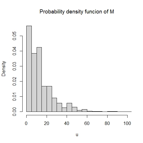
Formula (35) allows us to simulate independent observations on MM without generating all sample paths of the risk process and to plot the probability to survive, which is actually estimated via the empirical c.d.f. of MM. Moreover, we can estimate also its derivative, which coincides with the probability density function of MM.

Such simulation study was performed with sample size 10710^{7} and parameters λ0=10\lambda_{0}=10, λ1=11\lambda_{1}=11, λ2=12\lambda_{2}=12, ν1=1\nu_{1}=1, ν2=2\nu_{2}=2, ν3=ν4=3\nu_{3}=\nu_{4}=3, and c=97c=97. Then, ρ≈0.021\rho\approx 0.021, and μ=95\mu=95. Both plots are given on Figure 1.

Refer to caption
Refer to caption
Figure 1: Estimators of the probability to survive (left) and its derivative (right)

6 CONCLUSIONS

Analogous conclusions could be done for mathematical models of insurance businesses with more types of claims, more types of polices, and more types of shock event. The idea is to reduce them to the classical compound Poisson risk model.

Although the model is constructed by a multivariate counting processes, along the paper it is shown that the total claim amount process is stochastically equivalent to a univariate compound Poisson process. These allows us to reduce the considered risk model to a Cramer-Lundberg risk model, to use the corresponding results and to make the conclusions for the new model.

These results give us a different approach for estimation of the probability of ultimate ruin and its derivative.

Analogous results can be applied in queuing theory.

7 ACKNOWLEDGMENTS

The first author is partially supported by the project RD-08-144/01.03.2022 from the Scientific Research Fund in Konstantin Preslavsky University of Shumen, Bulgaria. Evelina Veleva thanks to the project No 2022-FNSE-04, financed by ”Scientific research” Fund of Ruse University.

References

  • [1] Asmussen, S., Albrecher, H. Ruin probabilities, Advansed Series on Statistical Science & Applied Probability, vol. 14, (2010) World Scientific.
  • [2] Beekman, J.A., Collective risk results, Transactions of the Society of Actuaries, vol.20, pp. 182–199, (1968).
  • [3] Cossette, H., Marceau, H., The discrete-time risk model with correlated classes of business, Insurance: Mathematics and Economics, vol.26(2), pp. 133–149, (2000).
  • [4] Gerber, H.U., An introduction to mathematical risk theory, SS Heubner Foundation Monograph Series, Monograph No. 8, (1979) University of Michigan.
  • [5] Gerber, H.U., Shiu, E.S.W., The joint distribution of the time of ruin, the surplus immediately before ruin, and the deficit at ruin, Insurance: Mathematics and Economics, vol. 21(2), pp. 129-137 (1997).
  • [6] Grandell, J., Aspects of risk theory, Springer Series in Statistics, (1992) Springer Verlag.
  • [7] Jordanova, P., Merging of bivariate Compound Poisson risk processes with shocks, MATTEX 2018 Conference proceedings, vol. 1, pp. 49–56, (1988).
  • [8] Jordanova, P., Veleva, E., Merging of bivariate Binomial risk processes with shocks, AIP Conference Proceedings, vol. …, pp. …–…, (2021).
  • [9] Kingman, J. F. C., Poisson Processes, Oxford studies in probability, (1991) Clanderon press, Oxford.
  • [10] Klugman, S. A., Pnjer, H., H., and Willmot, G. E., Loss models: from data to decision, (2012) John Wiley & Sons.
  • [11] Khinchine, A.Y., Mathematical theory of a stationary queue, Matematicheskii Sbornik, vol. 39(4):7384 (1932) (in russian).
  • [12] Kocherlakota, S., Kocherlakota, K., Bivariate Discrete Distributions, (1992) Marcel Dekker, New York.
  • [13] Mardia, K., V., Families of Bivariate Distributions, (1970) Charles Griffin and Sons, London.
  • [14] Marshall, A.W., Olkin, I., A multivariate exponential distribution, Journal of the the Americn Statistical Association, vol.62, pp. 30–44, (1967).
  • [15] Marshall, A.W., Olkin, I., Families of multivariate distributions, Journal of the the Americn Statistical Association, vol.83, pp. 834–841, (1988).
  • [16] Rolski, T., Schmidli, H., Schmidt, V., Teugels, J., Stochastic processes for insurance and finance, vol. 505 (1998) John Wiley and Sons.
  • [17] Sundt, B., Vernic, R., Recursions for convolutions and compound distributions with insurance applications, (2009) Springer Science & Business Media.
  • [18] Vernic, R., On the Evaluation of the Distribution of a General Multivariate Colleacite Model: Recursions versus Fast Fourier Transform, Risks, vol.6(3), 87, pp. 1–14, (2018), MDPI.