Numerically Robust Methodology for Fitting Current-Voltage Characteristics of Solar Devices with the Single-Diode Equivalent-Circuit Model

Mario Zinßer Affiliation: Zentrum für Sonnenenergie- und Wasserstoff-Forschung Baden-Württemberg (ZSW), Meitnerstraße 1, 70563 Stuttgart, Germany Affiliation: Light Technology Institute (LTI), Karlsruhe Institute of Technology (KIT), Engesserstraße 13, 76131 Karlsruhe, Germany Affiliation: Correspondence to Mario Zinßer via mario.zinsser@zsw-bw.de

2022 July 6^th

Abstract

For experimental and simulated solar cells and modules discrete current-voltage data sets are measured. To evaluate the quality of the device, this data needs to be fitted, which is often achieved within the single-diode equivalent-circuit model. This work offers a numerically robust methodology, which also works for noisy data sets due to its generally formulated initial guess. A Levenberg–Marquardt algorithm is used afterwards to finalize the fitting parameters. The source code and an executable version of the methodology are published under https://github.com/Pixel-95/SolarCell_DiodeModel_Fitting on GitHub. This work explains the underlying methodology and basic functionality of the program.

1 Introduction

Experimental and simulated solar devices yield a certain current under a given applied voltage and illumination. Due to the underlying semiconductor physics of p-n junctions, this relation is highly non-linear [1]. Most of these current-voltage (IV) curves can be described by a simple electronic model with a lumped series and shunt resistance, a diode, and an ideal current source. The numerical challenge is to find the five fitting parameters for all electric components within the single-diode equivalent-circuit model from a set of experimental data given at $n$ discrete voltages $V_{1}$ , …, $V_{n}$ and their corresponding current values $I_{1}(V_{1})$ , …, $I_{n}(V_{n})$ . There exist many algorithms in literature [2, 3, 4, 5] and even their errors are analysed [6]. However, the goal of this work is to find a numerically robust method that works also for IV data perturbed by noise effects, such as data outliers, sparse data sets, or higher voltages in modules instead of cells and hence a significantly higher diode ideality factor.

The following section will present the methodology of fitting, while the one after introduces an executable program capable of fitting measured data sets.

2 Methods

Figure 1: Single-diode equivalent-circuit model. While the photo current represents the generated current, the voltage-dependent shunt and diode currents flow in the opposing direction reducing the produced power.

In general, the current-voltage relation¹¹ 1 In this work, all currents are treated as absolute currents $I$ with the SI unit Amperes ( $\mathrm{A}$ ). However, the same methodology also works for current densities $j$ with the SI unit Ampere per square meter $\left(\frac{\mathrm{A}}{\mathrm{m}^{2}}\right)$ . of regular solar devices at the temperature $T$ as seen in Figure 1 can be described by the implicit relation [2]

$\displaystyle I(V)$	$\displaystyle=-I_{\mathrm{ph}}+I_{\mathrm{sh}}(V)+I_{\mathrm{d}}(V)$
	$\displaystyle=-I_{\mathrm{ph}}+\frac{V-I(V)\cdot R_{\mathrm{s}}}{R_{\mathrm{sh}}}$
	$\displaystyle\;\;\;\>\,+I_{0}\cdot\left(\exp\left(\frac{q_{\mathrm{e}}\cdot\left(V-I(V)\cdot R_{\mathrm{s}}\right)}{n_{\mathrm{d}}{k_{\mathrm{B}}}T}\right)-1\right).$	(1)

Here, $I_{\mathrm{ph}}$ is the generated photo current, $R_{\mathrm{s}}$ and $R_{\mathrm{sh}}$ the lumped resistances in series and shunt, $I_{0}$ the reverse saturation current, $n_{\mathrm{d}}$ the diode ideality factor, ${k_{\mathrm{B}}}$ the Boltzmann constant, and $q_{\mathrm{e}}$ the elementary charge.

By using the Lambert W function [7] it can be converted into an explicit equation. [8, 9, 10]

\displaystyle I(V)=\;

\displaystyle\frac{n_{\mathrm{d}}{k_{\mathrm{B}}}T}{q_{\mathrm{e}}R_{\mathrm{s}}}\cdot\mathcal{W}\left(f_{\mathrm{Lam}}\right)+\frac{V-R_{\mathrm{sh}}\cdot\left(I_{\mathrm{ph}}+I_{0}\right)}{R_{\mathrm{s}}+R_{\mathrm{sh}}},

(2)

where $\mathcal{W}\left(x\right)$ is the Lambert W function and

	$\displaystyle f_{\mathrm{Lam}}=\;$	$\displaystyle\frac{q_{\mathrm{e}}I_{0}R_{\mathrm{sh}}R_{\mathrm{s}}}{n_{\mathrm{d}}{k_{\mathrm{B}}}T\left(R_{\mathrm{s}}+R_{\mathrm{sh}}\right)}$
		$\displaystyle\cdot\exp\left({\frac{q_{\mathrm{e}}R_{\mathrm{sh}}\Big(R_{\mathrm{s}}\left(I_{\mathrm{ph}}+I_{0}\right)+V\Big)}{n_{\mathrm{d}}{k_{\mathrm{B}}}T\left(R_{\mathrm{s}}+R_{\mathrm{sh}}\right)}}\right).$		(3)

This section starts with the actual process of fitting and finishes with the calculation of the characteristic data, such as the open circuit voltage from the fitted parameters.

In Table 1, all variables used in this work are explained.

variable	meaning
$V$	voltage
$V_{i}$	$i$ -th voltage of the experimental data set to be fitted
$V_{\mathrm{oc}}$	open circuit voltage
$V_{\mathrm{MPP}}$	voltage at the maximum power point
$I$	current
$I_{i}$	$i$ -th current of the experimental data set to be fitted
$I_{\mathrm{ph}}$	generated photo current
$I_{\mathrm{d}}$	current flowing across the diode
$I_{\mathrm{sh}}$	shunt current
$I_{\mathrm{ph}}$	generated photo current
$I_{0}$	reverse saturation current
$I_{\mathrm{sc}}$	short circuit current
$I_{\mathrm{MPP}}$	current at the maximum power point
$P$	power
$P_{i}$	$i$ -th power of the experimental data set to be fitted (calculated from $V_{i}$ and $I_{i}$ )
$P_{\mathrm{MPP}}$	power at the maximum power point
$R_{\mathrm{s}}$	series resistance
$R_{\mathrm{sh}}$	shunt resistance
$n_{\mathrm{d}}$	diode ideality factor
$\mathrm{FF}$	fill factor
$q_{\mathrm{e}}$	elementary charge
${k_{\mathrm{B}}}$	Boltzmann constant
$\mathcal{W}(x)$	Lambert W function [7]
$\mathcal{L}_{i}$	function value of $\mathcal{W}(x)$ in the $i$ -th iteration of approximation
$R^{2}$	coefficient of determination
$n$	amount of experimental data points

Table 1: Table of all variables and symbols in this work. All current values can also be replaced by current density values.

2.1 Fitting Procedure

The fitting process is divided into two sections. The first one being the initial guess for the start values of the fitting parameters and the second one being the actual fitting algorithm itself. Since IV characteristics are highly non-linear, getting a sophisticated initial guess is crucial for the subsequent fitting algorithm and therefore is the most important task. As already described in the introduction, the goal of the outlined initial guess is not to be as precise as possible, but to be as robust and universal as possible.

2.1.1 Initial Guess

The initial guess for the fitting algorithm is obtained by the following procedure.

1.

As a first step, a cubic Savitsky-Golay filter [11] with a window size of 9 is applied to the experimental data in order to smooth data and not be sensitive to outlier data and noise. Moreover, the current values are eventually multiplied by $-1$ in order to put the data in the appropriate quadrant.
2.

The maximum power point (MPP) is roughly estimated as the discrete data point with the maximum power calculated via $P_{i}=V_{i}\cdot I_{i}$ .
3.

The open circuit voltage $V_{\mathrm{oc}}$ is estimated as the linear interpolation of last data point with a negative current and the first data point with a positive current. If there are only data points with negative currents it is calculated via $V_{\mathrm{oc}}=1.2\cdot V_{\mathrm{MPP}}$ .
4.

The diode ideality factor is estimated to be $n_{\mathrm{d}}=2\cdot\frac{V_{\mathrm{oc}}}{\left[\mathrm{Volt}\right]}$ .
5.

All data points with a voltage below 20 % of $V_{\mathrm{oc}}$ are fitted with a linear regression. The inverse slope is considered as the shunting resistance $R_{\mathrm{sh}}$ and the y-intercept as the photo current $I_{\mathrm{ph}}$ .
6.

The 5 data points with the largest voltage are fitted linearly. The inverse slope of the regression is taken as the initial guess for the series resistance $R_{\mathrm{s}}$ .
7.

Finally, the reverse saturation current is calculated by the diode equation (1) at $V=V_{\mathrm{oc}}$ and hence $I(V_{\mathrm{oc}})=0$ via $I_{0}=\frac{I_{\mathrm{ph}}-V_{\mathrm{oc}}/R_{\mathrm{sh}}}{\exp\left(q_{\mathrm{e}}V_{\mathrm{oc}}/(n_{\mathrm{d}}{k_{\mathrm{B}}}T)\right)-1}.$

2.1.2 Convergent Fitting Method

Starting from the initial guess described in the past section, the partial derivation with respect to all 5 fitting parameters are derived analytically via the Lambert W function. Using them, a Levenberg–Marquardt algorithm [12, 13] is used in order to perform a regression to all data points. Since the initial guesses for the photo current and the shunt resistance are typically accurate within a few percent, they are not fitted with the other parameters. Hence, only $I_{0}$ , $n_{\mathrm{d}}$ , and $R_{\mathrm{s}}$ are fitted in this subprocedure. At this point, the regression curve usually fits the data points very well. However, in a second procedure, all 5 parameters are fitted with the Levenberg–Marquardt algorithm to give the program the chance to adapt every parameter at the same time.

2.2 Calculate Characteristic Data

Once all fitted diode parameters $I_{\mathrm{ph}}$ , $I_{0}$ , $n_{\mathrm{d}}$ , $R_{\mathrm{s}}$ , and $R_{\mathrm{sh}}$ are determined, the solar parameters open circuit voltage $V_{\mathrm{oc}}$ , short circuit current $I_{\mathrm{sc}}$ , and fill factor $\mathrm{FF}$ need to be calculated. This section describes their direct determination from the fitting parameters.

2.2.1 Open Circuit Voltage $V_{\mathrm{oc}}$

At the open circuit point, the current $I(V)$ vanishes. Therefore, the open circuit voltage $V_{\mathrm{oc}}$ can be determined by Equation (1) via

\displaystyle V_{\mathrm{oc}}

\displaystyle=R_{\mathrm{sh}}(I_{\mathrm{ph}}+I_{0})-\frac{n_{\mathrm{d}}{k_{\mathrm{B}}}T}{q_{\mathrm{e}}}\cdot\mathcal{W}\left(f_{\mathrm{Lam}}^{\mathrm{oc}}\right)

(4)

with

\displaystyle f_{\mathrm{Lam}}^{\mathrm{oc}}

\displaystyle=\frac{q_{\mathrm{e}}I_{0}R_{\mathrm{sh}}}{n_{\mathrm{d}}{k_{\mathrm{B}}}T}\cdot\exp\left(\frac{q_{\mathrm{e}}R_{\mathrm{sh}}(I_{\mathrm{ph}}+I_{0})}{n_{\mathrm{d}}{k_{\mathrm{B}}}T}\right).

(5)

If the exponent in Equation (5) is larger than the maximum exponent of double value ( $\sim 308$ for IEEE double precision [14]) the Lambert W function $\mathcal{W}\left(f_{\mathrm{Lam}}\right)$ is calculated via the approximation for large numbers given in Appendix A.

2.2.2 Short Circuit Current $I_{\mathrm{sc}}$

The short circuit point is defined as the state without an externally applied voltage and therefore shorted contacts. Hence, $V=0$ is be plugged into Equation (2) and can be solved via the Lambert W function yielding

\displaystyle I_{\mathrm{sc}}

\displaystyle=\frac{n_{\mathrm{d}}{k_{\mathrm{B}}}T}{q_{\mathrm{e}}R_{\mathrm{s}}}\cdot\mathcal{W}\left(f_{\mathrm{Lam}}^{\mathrm{sc}}\right)-\frac{R_{\mathrm{sh}}(I_{\mathrm{ph}}+I_{0})}{R_{\mathrm{sh}}+R_{\mathrm{s}}}

(6)

with

\displaystyle f_{\mathrm{Lam}}^{\mathrm{sc}}

\displaystyle=\frac{q_{\mathrm{e}}I_{0}R_{\mathrm{sh}}R_{\mathrm{s}}}{n_{\mathrm{d}}{k_{\mathrm{B}}}T(R_{\mathrm{sh}}+R_{\mathrm{s}})}\cdot\exp\left(\frac{q_{\mathrm{e}}R_{\mathrm{sh}}R_{\mathrm{s}}(I_{\mathrm{ph}}+I_{0})}{n_{\mathrm{d}}{k_{\mathrm{B}}}T(R_{\mathrm{sh}}+R_{\mathrm{s}})}\right).

(7)

2.2.3 Maximum Power Point MPP

In order to obtain the power $P$ from a current-voltage characteristic, the current $I$ is multiplied by the voltage $V$ . The maximum power point (MPP) is defined as the point in the IV curve with the highest produced power. To calculate the MPP, Equation (2) is multiplied by $V$ and afterwards the maximum is determined via

\displaystyle\frac{\mathrm{d}P(V)}{\mathrm{d}V}=\frac{\mathrm{d}(I(V)\cdot V)}{\mathrm{d}V}=0

(8)

by using the Newton-Raphson method. This yields the MPP voltage $V_{\mathrm{MPP}}$ , resulting in the MPP current $I_{\mathrm{MPP}}=I(V_{\mathrm{MPP}})$ via Equation (2) and MPP power $P_{\mathrm{MPP}}=P(V_{\mathrm{MPP}})$ .

2.2.4 Fill Factor FF

Based on the calculation of the MPP, the fill factor $\mathrm{FF}$ is the area ratio of the two rectangles drawn from the origin towards the MPP and from the origin towards the axis intersects. It is therefore given as

\displaystyle\mathrm{FF}

\displaystyle=\frac{V_{\mathrm{MPP}}I_{\mathrm{MPP}}}{V_{\mathrm{oc}}I_{\mathrm{sc}}}.

(9)

2.2.5 Coefficient of Determination $R^{2}$

To be able to tell how good the fit matches the experimental data, a gauge is introduced. This happens to be the coefficient of determination $R^{2}$ and is defined as

\displaystyle R^{2}

\displaystyle=1-\frac{\sum_{i}^{n}\Big(I_{i}(V_{i})-I(V_{i})\Big)^{2}}{\sum_{i}^{n}\Big(I_{i}(V_{i})-I_{\mathrm{mean}}\Big)^{2}},

(10)

where

\displaystyle I_{\mathrm{mean}}

\displaystyle=\frac{1}{n}\sum_{i}^{n}I_{i}(V_{i}).

(11)

It typically ranges from 0 (fit always predicts $I_{\mathrm{mean}}$ ) to 1 (fit perfectly matches all given data points). A negative $R^{2}$ means that the model is even worse than the mean value.

3 Program

The executable program of the described algorithm is adaptable to certain circumstances as seen in Figure 2. Both formatting preferences and units of the voltage and the current (density) can be selected. Moreover, a certain temperature is required.

Refer to caption — Figure 2: Screenshot of the preferences section. Besides the format symbols and the temperature, the units of the voltage and the current or current density can be selected.

The main window of the program is shown in Figure 3. Within the left side, the experimental current-voltage data can be inserted.

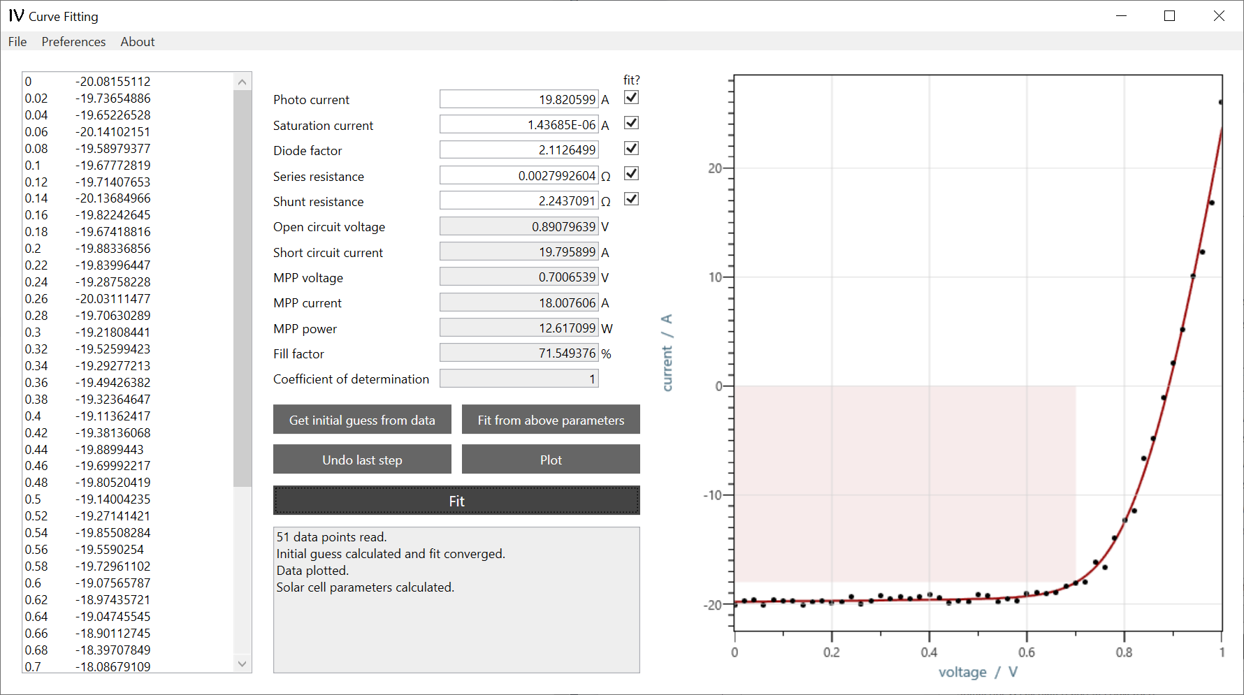
The middle section shows the fitted diode parameters and the calculated characteristic parameters. Furthermore, there are all buttons to operate the program. The main button "Fit" simply fits the experimental data on the left with the above described methodology. There is also the possibility to only get the initial guess from the data. The button "Fit from above parameters" does not calculate an initial guess but rather takes the already defined diode parameters as starting values. The check boxes determine which parameters are fitted.

On the right side, the experimental data is plotted as black points and the fitted curve as red line. Additionally, a red box represents the covered power at the MPP.

The source code and executable file can be found under https://github.com/Pixel-95/SolarCell_DiodeModel_Fitting within a GitHub repository.

4 Conclusion

This work introduces a methodology of fitting current-voltage characteristics of solar devices with the single-diode equivalent-circuit model. Due to the general calculation of the initial guess it is applicable even to perturbed data sets of cells and modules. Afterwards a Levenberg–Marquardt algorithm is applied in order to convergently determine the required fitting parameters.

5 Acknowledgements

The author acknowledges fruitful and productive discussions with Tim Helder, Erwin Lotter, and Andreas Bauer. This work was inspired and supported by the German Federal Ministry for Economic Affairs and Climate Action (BMWK) under the contract number 0324353A (CIGSTheoMax).

Appendix A Calculating the Lambert W function

As the Lambert W function $\mathcal{W}\left(x\right)$ [7] is defined via the inverse function of the transcendental equation

\displaystyle\mathcal{W}\left(x\right)\cdot e^{\mathcal{W}\left(x\right)}

\displaystyle=x,

(12)

it is necessary to calculate it numerically. An efficient method to do so is Halley’s method [15] in order to iteratively approximate its value. The rough approximation

\displaystyle\mathcal{L}_{0}=\frac{3}{4}\log(x+1)

(13)

is used as an initial guess for the function value $\mathcal{L}$ and by using the first and second derivatives, the iteration procedure

\displaystyle\mathcal{L}_{i+1}=\mathcal{L}_{i}-\dfrac{\mathcal{L}_{i}\cdot e^{\mathcal{L}_{i}}-\mathcal{L}_{i}}{e^{\mathcal{L}_{i}}\cdot(\mathcal{L}_{i}+1)-(\mathcal{L}_{i}+2)\cdot\dfrac{\mathcal{L}_{i}e^{\mathcal{L}_{i}}-\mathcal{L}_{i}}{2\mathcal{L}_{i}+2}}

(14)

can be derived. Equation (14) is iteratively executed $\left\lceil\frac{1}{3}\log_{10}(x)\right\rceil$ times with a minimum of four iterations. This ensures a sufficiently precise accuracy for double precision with a 52 bit long mantissa. [14]

For too large values of $x$ , the numbers in equation (14) become too large to be handled by a regular double precision. Therefore, a simple approximation for large input values is used [16]. By using the auxiliary variable

\displaystyle w

\displaystyle=\log\left(x\right)

(15)

without any physical meaning, the function value can be approximated via

\displaystyle\mathcal{W}\left(x\right)=w-\log(w)+\frac{\log(w)}{w}+\mathcal{O}\left(\left(\frac{\log(w)}{w}\right)^{2}\right).

(16)

References

[1] Shockley, W. The Theory of p-n Junctions in Semiconductors and p-n Junction Transistors. Bell System Technical Journal 28, 435–489 (1949).
[2] Hegedus, S. S. & Shafarman, W. N. Thin-film solar cells: device measurements and analysis. Progress in Photovoltaics: Research and Applications 12, 155–176 (2004).
[3] Diantoro, M. et al. Shockley’s equation fit analyses for solar cell parameters from IV curves. International Journal of Photoenergy 2018 (2018).
[4] Toledo, F. J., Blanes, J. M. & Galiano, V. Two-step linear least-squares method for photovoltaic single-diode model parameters extraction. IEEE Transactions on Industrial Electronics 65, 6301–6308 (2018).
[5] Mehta, H. K., Warke, H., Kukadiya, K. & Panchal, A. K. Accurate expressions for single-diode-model solar cell parameterization. IEEE Journal of Photovoltaics 9, 803–810 (2019).
[6] Phang, J. C. H. & Chan, D. S. H. A review of curve fitting error criteria for solar cell I-V characteristics. Solar Cells 18, 1–12 (1986).
[7] Lamberti, J. H. Observationes variae in mathesin puram. Acta Helvetica Physico-Mathematico-Anatomico-Botanico-Medica 3, 128–168 (1758).
[8] Jain, A. & Kapoor, A. Exact analytical solutions of the parameters of real solar cells using Lambert W-function. Solar Energy Materials and Solar Cells 81, 269–277 (2004).
[9] Ghani, F., Duke, M. & Carson, J. Numerical calculation of series and shunt resistances and diode quality factor of a photovoltaic cell using the Lambert W-function. Solar Energy 91, 422–431 (2013).
[10] Zinßer, M. et al. Finite Element Simulation of Electrical Intradevice Physics of Thin-Film Solar Cells and Its Implications on the Efficiency. IEEE Journal of Photovoltaics 12, 483–492 (2022).
[11] Savitzky, A. & Golay, M. J. E. Smoothing and differentiation of data by simplified least squares procedures. Analytical chemistry 36, 1627–1639 (1964).
[12] Levenberg, K. A method for the solution of certain non-linear problems in least squares. Quarterly of Applied Mathematics 2, 164–168 (1944).
[13] Marquardt, D. W. An algorithm for least-squares estimation of nonlinear parameters. Journal of the Society for Industrial and Applied Mathematics 11, 431–441 (1963).
[14] Standard for Floating-Point Arithmetic (IEEE 754). IEEE SA - The IEEE Standards Association (2019).
[15] Alefeld, G. On the convergence of Halley’s Method. The American Mathematical Monthly 88, 530–536 (1981).
[16] Hoorfar, A. & Hassani, M. Approximation of the Lambert W function and hyperpower function. Research Report Collection 10 (2007).