The Bounded Beam Search algorithm for the Block Relocation Problem
Abstract
In this paper we deal with the restricted Block Relocation Problem. We
present a new lower bound and a heuristic approach for the problem.
The proposed lower bound can be computed in polynomial time and
it is provably better than some previously known lower bounds.
We use it within a bounded beam search algorithm to solve the Block Relocation Problem
and show that the considered heuristic approach outperforms the other existing
algorithms on most of the instances in the literature.
In order to test the approaches on real-size dimensions,
new large instances of the Block Relocation Problem are also introduced.
Keywords: Block Relocation, Container Relocation, Beam Search, Lower Bound, Heuristics, Realistic Instances.
This is the postprint version of the article “Bacci, T. , Mattia, S. , Ventura, P. (2019). The bounded beam search algorithm for the block relocation problem. Computers & Operations Research, 103 , 252–264 .” The published version is available at https://doi.org/10.1016/j.cor.2018.11.008.
1 Introduction
Let be a system (yard) defined by stacks of capacity (in terms of available slots/tiers) and let be a set of blocks located in the slots of the stacks. A reshuffle operation (or simply a reshuffle or a relocation) is a movement of a block from a stack to another, while a retrieval is a movement of a block from a stack to the outside of the system. The stacks can store blocks according to a last-in / first-out policy. In a stack, only the topmost block is accessible and, when a block has to be retrieved, all the blocks above it have to be reshuffled. When a block is reshuffled and moved in one of the other stacks of the yard, it has to be allocated in the first slot available from the bottom to the top.
The Block Relocation Problem (BRP) consists in deciding where to reallocate every block that is moved by a reshuffle operation, in order to minimize the total number of reshuffles needed to retrieve all the blocks according to the retrieval order (1,…,n). Observe that such minimum is lower bounded by the number of blocking blocks of , i.e., those located in any slot above a block with higher retrieval priority. Figure 1 gives an example of the BRP with a system defined by stacks, available slots for each stack, and blocks. Starting from the initial yard, where blocks 5 and 6 are blocking, the sequence of movements of an optimal solution is reported. At each step, the next block to be moved with a reshuffle or a retrieval operation is highlighted in gray. The minimum number of reshuffles required is three: block 6 is reshuffled in order to retrieve block 1; block 5 is reshuffled to retrieve block 2; we then reshuffle block 6 to retrieve block 4. Since BRP generalizes the Bounded Coloring Problem (also known as Mutual Exclusion Scheduling) on permutation graphs, it is known to be NP-hard for any fixed . For some complexity results on BRP, Bounded Coloring and related problems, see Caserta et al. 2012, Jansen 2003, Bonomo et al. 2011, and Bacci et al. 2017.
A real world application of the BRP arises in the logistics of containers in a terminal. A container terminal is an area where containers are stored and transshipped between different transport vehicles, such as cargo ships, trains, trucks, and where they are stacked because of the limited storage space. The storage area (yard) is often divided into groups of stacks of containers, called bays, and containers are moved by yard cranes. The movements of containers may occur within the same bay or between different bays (Lee and Lee 2010). Typically, a container yard stores at the same time thousands of containers grouped into hundreds of stacks with a storage capacity which may be up to 10 slots (Günter and Kim 2005). Since a stack is accessible only from the top, when a container is required outside of the storage area, any container located above it has to be moved to another stack by a yard crane with a reshuffle operation. Reshuffle operations are time-consuming and they have to be avoided as much as possible. In this scenario, the Block Relocation Problem consists in finding a way to retrieve, in a given order, all the containers in the container yard so to minimize the number of reshuffle operations. Throughout the paper, the words container and block will be used interchangeably.
In the literature, two variants of the BRP are studied: restricted and unrestricted. In the restricted version, it is allowed to reshuffle only blocks located above the next one to be retrieved, while, in the unrestricted case, any block can be reshuffled. In this work, we focus on the first variant. Readers interested in the unrestricted version can refer to Forster and Bortfeldt 2012, Petering and Hussein 2013, Tanaka and Mizuno 2015, and Tricoire et al. 2018.
The best exact approaches proposed for the restricted BRP allow to solve instances with up to 70 containers (Zhu et al. 2012 and Tanaka and Takii 2016), that is, in most cases, far away from the dimension of a real world scenario (Lee and Lee 2010). Therefore, a huge amount of heuristics have been proposed in the literature. Here we describe a new beam search approach, the Bounded Beam Search algorithm, and we compare it with the other methods in the literature, showing that it outperforms most of the existing approaches. In the Bounded Beam Search algorithm we make use of a new lower bound for BRP, denoted as the Unordered Blocks Assignment Lower Bound. We compare it with other lower bounds in the literature and prove that it theoretically dominates the two most used ones. In addition, we introduce a new set of instances, large enough to represent real scenarios.
In Section 2, we give a survey of the literature on BRP, focusing on the heuristic procedures (Section 2.2) and on the lower bounds (Section 2.3); some variants of the BRP are described in Section 2.4. In Section 3, we introduce the Unordered Blocks Assignment Lower Bound. In Section 4, we describe the Bounded Beam Search heuristic algorithm in details. In Section 5, we describe the test bed used in the computational experiments. In Section 7, we study how the behavior of the Bounded Beam Search algorithm changes according to some parameters. In Section 8, we compare the performances of the Bounded Beam Search procedure with the best heuristic methods taken from the literature on different sets of instances. Finally, in Section 9, we present our comments and conclusions.

2 Literature review
A huge amount of literature concerning storage yard operations in container terminals has been proposed in the last two decades, as described in the recent surveys by Carlo et al. 2014 and Lehnfeld and Knust 2014. Below we review the literature for the BRP and some of its variants, focusing on heuristic approaches and lower bounds for the problem.
2.1 Exact approaches
The exact approaches for the problem can be distinguished into methods based on Integer Linear Programming (ILP) formulations (Caserta et al. 2012, Wan et al. 2009, Zehendner and Feillet 2014, Zehendner et al. 2015) and search-based methods (Kim and Hong 2006, Wu and Ting 2010, Unluyurt and Aydin 2012, Zhu et al. 2012, Izquierdo et al. 2014, Tanaka and Takii 2016, Izquierdo et al. 2015, Ku and Arthanari 2016b). ILP based methods can solve only instances up to 30 blocks, while search-based exact algorithms can tackle instances with up to 70 blocks (see Tanaka and Takii 2016).
2.2 Heuristic algorithms
Many heuristic procedures have been proposed for the BRP. These algorithms can be grouped into fast or slow methods. In the first group we include all the algorithms based on a simple greedy approach, while the second group contains procedures that are more sophisticated or structured. The fast approaches include the following algorithms: the Lowest Position heuristic (Zhang 2000); the Reshuffle Index heuristic (Murty et al. 2005); the heuristic rule based on the Expected Number of Additional Relocations (Kim and Hong 2006); the Extended Lowest Position heuristic, the Extended Reshuffle Index heuristic, the Extended heuristic based on the Expected Number of Additional Relocations (Wan et al. 2009); the Reshuffle Index with Look-ahead heuristic (Wu and Ting 2010); the heuristic procedure proposed in Caserta et al. 2012; the Lowest Absolute Difference heuristic, the Group Assignment Heuristic by Wu and Ting 2012; the Greedy1 heuristic, the Difference1 heuristic (Unluyurt and Aydin 2012); the Probe Restricted 1 heuristic, the Probe Restricted 2 heuristic, the Probe Restricted 3 heuristic, the Probe Restricted 4 heuristic (Zhu et al. 2012); the Chain heuristic, the ChainF heuristic (Jovanovic and Voß 2014). Below we briefly describe such fast procedures.
In the Lowest Position heuristic the next block that has to be reshuffled is assigned to the stack that has the highest number of empty slots. The Reshuffle Index heuristic assigns a reshuffled block to the stack with the minimum number of containers that have an higher priority (a lower index). The heuristic rule based on the Expected Number of Additional Relocations assigns the next block to be reshuffled to the stack with the minimum expected number of additional relocations. The Extended Lowest Position heuristic, the Extended Reshuffle Index heuristic, the Extended heuristic based on the Expected Number of Additional Relocations are modified (refined) versions of the Lowest Position heuristic, the Reshuffle Index heuristic and the heuristic rule based on the Expected Number of Additional Relocations, respectively. In particular, the novelty consists of assigning each reshuffled block to the stack that minimizes an upper bound computed using the original heuristic. the Reshuffle Index with Look-ahead heuristic is also a development of the Reshuffle Index procedure and they differ in the rule for breaking ties. In the heuristic procedure proposed in Caserta et al. 2012 a block is assigned to the stack ; otherwise to the stack . Here and in the following, is the block with the minimum index among those allocated in stack . We note that this procedures, the Lowest Absolute Difference heuristic and the Probe Restricted 3 heuristic correspond to the same algorithm. To move the reshuffled container in a stack , Difference1 considers (in this order) the following three criteria: i) ; ii) , where is the topmost block of ; iii) . The Probe Restricted 1 heuristic and the Lowest Position procedure differ only in the rule adopted for breaking ties. In the Probe Restricted 2 heuristic, the next block to be reshuffled is assigned to the stack that maximizes . As in Difference1, also in the Probe Restricted 4 heuristic the stack is selected iteratively applying different criteria on . Differently from the approaches described so far, the Group Assignment Heuristic, ChainF, Chain, and Greedy1 consider, at each step, not only the next block that has to be reshuffled, but a subset of the blocking blocks above the next one to be retrieved. Chain and ChainF iteratively reshuffle the block of in consecutive pairs, whereas the Group Assignment Heuristic and Greedy1, assign all the blocks in at the same time.
The slow approaches include the following algorithms: the Minimum Reshuffle Integer Program heuristic (Wan et al. 2009); the Tabu Search heuristic by Wu et al. 2010; the Beam Search heuristic by Wu and Ting 2010; the Corridor Method heuristic (Caserta et al. 2011); the Matrix-Algorithm heuristic (Caserta et al. 2009); the three phase-heuristic by Lee and Lee 2010; the iterative deepening A* restricted heuristic (Zhu et al. 2012); the depth-first branch & bound heuristic (Ku and Arthanari 2016b).
The Minimum Reshuffle Integer Program heuristic is based on an Integer Linear Programming formulation, where a parameter indicates that such model minimizes the total number of reshuffles in retrieving the first containers. The Tabu Search heuristic implements a tabu search approach. The Beam Search heuristic is a beam search algorithm that uses the Reshuffle Index heuristic to compute the upper bounds. The basic idea of Corridor Method is to use an exact method over restricted portions of the solution space in order to find good feasible solutions. Zhu et al. 2012 noted that it may provide infeasible solutions. The Matrix-Algorithm explores all the configurations obtained by performing one reshuffle and by assigning to each child a score computed by a fast heuristic. Then, it randomly selects the next node to be explored. Its performances benefit from a smart binary encoding of the stacking area. The three phase-heuristic operates according to three phases: initially, a first feasible solution is obtained by a greedy procedure; then, an ILP formulation is used to try reducing the number of reshuffles; finally, another ILP is used to reduce the total time. The iterative deepening A* restricted heuristic is an implementation of the iterative deepening A* approach, applied to the restricted BRP. It is an exact method, that can be turned in a heuristic one, by setting a time limit. The depth-first branch & bound heuristic is obtained by fixing a time limit to an exact search based algorithm, which uses an abstraction method to reduce the solution space.
2.3 Lower bounds
There are few contributions in the literature related to lower bounds for the restricted BRP. Kim and Hong 2006 introduce a lower bound (referred in the literature as LB1, see Zhu et al. 2012) which derives from the simple observation that each blocking container has to be reshuffled at least once.
Zhu et al. 2012 present a lower bound (LB3) that can be calculated according to the following iterative procedure. Set . Then, for , consider container that has to be retrieved and let be the set of containers blocking . For each of these containers that will necessarily be blocking after its relocation, the variable is increased by 1. The yard at iteration is obtained by removing all the blocks in . Then, the value of LB3 is LB1 + .
The lower bound LB4, introduced by Tanaka and Takii 2016, is a refinement of LB3. However, while LB1 and LB3 can be calculated in polynomial time, the algorithm for computing LB4 is exponential in the number of blocks.
2.4 Related problems
The Container Pre-Marshalling Problem (CPMP, Lee and Hsu 2007) has several common aspects with the BRP. As in the latter, in the CPMP a set of containers, each of them having a retrieval priority, are located in a yard composed by a set of stacks with a given maximum height. The difference with BRP is that the blocks are not removed from the yard and only reshuffle operations are allowed. Here one has to reorder the blocks of the initial configuration so to obtain a yard without blocking blocks, with a minimum number of reshuffles. The CPMP has been largely studied in the literature and several heuristic algorithms and exact approaches have been presented (Hottung and Tierney 2016, Tanaka and Tierney 2018, Jovanovic et al. 2017). Another variant of BRP is the Blocks Relocation Problem with Batch Moves where more than one container at a time can be retrieved from the yard or moved between two stacks (Zhang et al. 2016).
Several robust variants of BRP are also studied: they include the Online Container Relocation Problem (Zehendner et al. 2017), in which the retrieval order is known only for a subset of the containers allocated in the initial configuration and the Container relocation problem with time windows (Ku and Arthanari 2016a), where the containers are divided into groups and it is given a retrieval order among the groups, but not among the blocks belonging to the same group.
3 A new lower bound for the BRP
In this Section, we present a new lower bound, called Unordered Blocks Assignment Lower Bound (UBALB), for the restricted BRP. A preliminary version of this contribution can be found in Bacci et al. 2018.
In the following we show that such a lower bound can be computed by iteratively solving a relaxation of the Generalized Blocking Items Problem (GMBIP) defined below. Given a yard composed by stacks of height , let be the block located in the -th slot of stack ( if the position is empty). Suppose to have a set of blocks that have to be allocated in the yard, according to a given order (denote by the -th block to be located) and let be the yard obtained from after placing these blocks. is said to be -feasible if it is compatible with , i.e., for each couple with , is not located above . Furthermore, a block is -blocking if it is located above block and it is blocking if it is -blocking for some . Given an input instance defined by (, , ), the GMBIP consists of finding a -feasible that minimizes the total number of blocking blocks. The optimal value is denoted by .
Lemma 1.
GMBIP is NP-hard.
Proof.
It contains the Minimum Blocking Items Problem (MBIP) as special case. Indeed, in MBIP the initial yard is assumed to be empty. MBIP is known to be NP-hard (Bacci et al. 2017). ∎
The solution of GMBIP can be used to obtain a lower bound for BRP, as we explain in the following.
Given a set of blocks located in a yard , let be obtained from by removing the block located in stack and the set of -blocking blocks (let be the order given by taking them from the top to the bottom), for each . It is worth observing that: (i) is the empty yard; (ii) block may not be present in ; and (iii) each block in has to be reshuffled at time . Furthermore, a block in may become blocking again after its reshuffle. The minimum number of such blocks is , where is obtained from by removing stack .
A lower bound for the BRP instance defined by is then given by the following equation:
| (1) |
Since GMBIP is NP-hard, the lower bound given by equation (1) is hard to compute in general. All the lower bounds for the BRP presented in the literature are, indeed, derived from (1) substituting, at each iteration , with some lower bound.
Kim and Hong 2006 compute LB1 by setting . For calculating LB3, Zhu et al. 2012 relax both the order and the capacity of the stacks. Tanaka and Takii 2016 only relax the capacity restriction on the stacks. We denote the optimal values of the corresponding relaxed problems by and respectively. Note that the algorithm presented by Zhu et al. 2012 to calculate runs in , whereas the one by Tanaka and Takii 2016 for requires steps. In the following, we say that a certain lower bound A dominates another lower bound B if, for every input instance, the value of A is not less than the value of B. Since it holds that: (i) LB3 dominates LB1; (ii) LB4 dominates LB3.
Here we introduce a new lower bound based on a relaxation GMBIPB of GMBIP, where the final matrix does not need to be -feasible. Let be the optimal value of GMBIPB.
Theorem 1.
The following holds: (i) the Unordered Blocks Assignment Lower Bound dominates LB3; (ii) neither LB4 dominates the Unordered Blocks Assignment Lower Bound nor the opposite.
Proof.
(i). Trivially, for any , .
In fact, the former relaxes both the -feasibility and constraints on the height of the stacks, whereas the latter only relaxes the -feasibility.
(ii). Figure 2 shows an instance of BRP where
LB4 has a value that is strictly less than the one of the Unordered Blocks Assignment
Lower Bound,
while Figure 3 represents an instance where the opposite relation
holds.
The figures depict the initial yard of the corresponding BRP problem on the left side.
In both cases, it is easy to see that for any .
Instead, in the first case we have , whereas in the second case .
The corresponding computation is reported on the right side of the figures.
As a consequence, in the first example, the value of LB4 is strictly less
(strictly greater, in the second case) than the one of the Unordered Blocks Assignment
Lower Bound.
Notice that, in Figure 2, the optimal configuration for , exceeds the capacity of the first stack.
∎


In the following we present an algorithm for solving .
Let , be the number of available empty slots of stack of and let be the minimum index of a block located in .
Algorithm 1
GMBIPB can be seen as a minimum cost assignment problem, where each block has to be assigned to some stack with . For each and , assigning to has cost 1, if , and 0 otherwise. Given , , , and , an instance of such assignment problem is denoted by ASS.
Theorem 2.
Algorithm 1 solves GMBIPB in .
Proof.
Given an input instance defined by a quadruple , we first prove that Algorithm 1 produces an optimal solution to the equivalent problem ASS. In the following, let and denote the solution provided by Algorithm 1 and an optimal solution to ASS, respectively. According with this notation, () indicates that block is located in stack ( is assigned to , respectively). Assume that is not and let be smallest index such that and with . We will show that we can produce another optimal solution where is assigned to . Indeed, let be such that , , and for all the other entries . Then two cases can occur. Case a): is feasible. Case b): is infeasible. In the latter case, since is feasible, it follows that, in , stack exceeds its capacity . Then observe that, since , the number of blocks in that are assigned to stack (both in as well as in ) is strictly less that . Therefore, there exists such that . Hence, we can construct a feasible matrix from , by setting and . Now, in order to prove that (Case a)) or (Case b)) is still optimal, we distinguish two sub-cases. First consider . Then, for Case a), it follows that is optimal. For Case b), observe that, as , then and, consequently, . Therefore, and is optimal. Now assume . Observe that , otherwise, for steps 6-7 of Algorithm 1, would have been assigned to stack instead of . This proves that, in Case a), is optimal. For Case b), notice that , otherwise, for steps 8-9 of Algorithm 1, again would have been assigned to stack . As a consequence, . Therefore, also in this case, and is optimal.
Finally, we analyze the computational complexity of the algorithm. Ordering the blocks of requires steps, while the stacks can be ordered in . Then, loop 4-12 is repeated times and, at each iteration, stack can be found in constant time. Hence the overall complexity is . ∎
4 A beam search algorithm for the BRP: the general scheme
Beam Search is a classic meta-heuristic based on an iterative enumeration of the feasible solutions that are represented by the leaves of an enumeration tree. Such an enumeration is not complete because the number of descendants of each node is bounded by a parameter . The main ingredients of the approach are then: an algorithm to calculate an upper bound UB(Y) for the value of the best solution that can be obtained by each node Y of the tree, and a value for the parameter . Therefore, for each node of the enumeration tree, the algorithm generates only the best (according to the value UB(Y)) descendants.
Here we present an improved beam search algorithm, called Bounded Beam Search, for the BRP. With respect to the standard beam search framework, we also make use of an algorithm to calculate a lower bound LB(Y) for the value of the best solution associated with each node Y. Such a value will be used both to select the best descendants to be generated and to further restrict the search space. In the following, we will describe the Bounded Beam Search procedure in more details. Algorithm 2 reports the pseudocode of the algorithm.
Algorithm 2
The algorithm proceeds by iteratively constructing the levels of the enumeration tree. Each level contains the nodes (yards) that can be obtained from the starting yard () by performing exactly reshuffle operations. The value of the current best solution is stored in the variable . The algorithm terminates when it constructs an empty level.
At each generic iteration , we consider all the nodes and proceed as follows: we first remove from all the blocks that can be retrieved without requiring a reshuffle operation (procedure RETRIEVAL). Then, let be the incumbent block of that has to be reshuffled, construct all yards , each associated with the movements of to feasible (not full) stacks of the yard, and compute and . Observe that has been obtained from the starting yard by performing reshuffles. Therefore, represents an upper bound on the value of the optimal solution of the problem. Then, in case, update the current value. All the nodes obtained in this way define the set of candidate descendants. Now, in order to select the nodes of that will be used to construct the next level , we first order them according to the values of the upper bound (in case of ties, we use to define a priority). Then, we select the first nodes according to this order. Finally, we remove from this set the nodes with , since they cannot generate a solution with a better value than .
The performances of the Bounded Beam Search heuristic strongly depend on the choice of the algorithms used to calculate and , as well as the value of parameter . Indeed, an accurate procedure for determines a more effective selection of the nodes that are generated and, then, hopefully, a better final solution. On the other hand, a good value of helps to reduce the solution space and, therefore, to decrease the total computing time. Clearly, it is usually the case that more accurate algorithms for the evaluation of and require more computational time. Moreover, an higher value for enlarges the search space (and then the probability to find a good solution) but also increases the total requested time. Then it is important to consider all such aspects to obtain good performances that balance quality and time. In Section 7, we discuss how to tune these parameters in an efficient way.
| Name | Authors |
|---|---|
| group 1 | Wan et al. 2009 |
| group 2 | Wu and Ting 2010 |
| group 3 | Lee and Lee 2010 |
| group 4 | Caserta et al. 2011 |
| group 5 | Unluyurt and Aydin 2012 |
| group 6 | Zhu et al. 2012 |
5 Description of the Data Set
We considered several sets of instances presented in the literature, divided into six groups that are resumed in Table 1. In the following, we first discuss datasets that are already available. Then we introduce the new set of instances lbri. The set lbri and the instances of group 1,…, group 6 are available at Bacci 2017.
group 1 is defined by the instances presented in Wan et al. 2009, all with six stacks of height between two and five. The storage densities of the stacks are classified as light (L), medium (M) and heavy (H), according to the percentage of operating capacity taken up. In particular, an instance with stacks of height is light if the number of blocks is , is medium if , and heavy if . In total, 12 combinations of stack sizes and storage densities are considered, each composed by 50 instances.
The instances of group 2 (Wu and Ting 2010) are grouped according to the number of stacks and height . Therefore, we have 100 problem classes, each with 40 instances. For each instance, the number of blocks .
The instances of group 3 (Lee and Lee 2010) are defined on multiple bays yards. Here, we consider only the subset of the 70 Individual ones, i.e., those where the blocks have distinct priorities. The instances can be Random (R), when the blocks are randomly located in the available slots, or Upside down (U), when blocks with higher retrieval priority are located in the lower slots of the stacks. All of them have up to 10 bays, , , and . Here we allow reshuffles of blocks between different bays: therefore, an instance with 10 bays and 16 stacks is equivalent to an instance with 1 bay and 160 stacks.
group 4 includes a set of 880 instances introduced in Caserta et al. 2011. Such instances are randomly generated with , and .
The 8000 instances of group 5 (Unluyurt and Aydin 2012) are generated with , and different densities of the blocks. They can be balanced (b), if the stacks have the same number of stored blocks, or unbalanced (u).
In group 6, we consider the 12500 instances described in Zhu et al. 2012. Such instances are grouped into 125 classes of size 100, according to the values of , , and .
We now introduce a new set of instances, the Large Block Relocation Instances (lbri), that we generated in order to evaluate the performances of the Bounded Beam Search algorithm on a realistic-sized test bed. Indeed, except for the ones of group 3 and group 4, the largest yards considered in the literature have a size of at most 12 stacks of height 12 and less than 140 blocks. This is far away from a realistic scenario, where a yard is usually defined by hundreds of stacks with thousands of blocks. The procedure implemented to generate the new instances follows the scheme introduced in Zhu et al. 2012. Here the authors show that it is always possible to retrieve all the blocks of a yard with stacks of height and blocks if any block is located in a slot such that . Then, for any triple , with , the instance generation procedure is the following: we first randomly order the blocks and then, according to this order, we iteratively assign each block to the first available slot of an available randomly selected stack. If the yard generated this way does not fit the feasibility condition defined above, then it is discarded and regenerated. The set lbri consists of 8400 instances, 100 for each triple , and .
6 Computing the Unordered Blocks Assignment Lower Bound
Here we test the proposed Unordered Blocks Assignment Lower Bound and compare the results with the ones obtained by the other lower bounds in the literature, namely LB1, LB3, LB4. Such comparison is reported in Table 2. Each row of the table represents a dataset. Columns LB1, LB3, LB4, and UBALB report average lower bounds (column Value) and computing times (column Time) on the instances of the considered dataset. The symbol is used to indicated that some instances of the corresponding group could not be solved within the time limit of one hour by the considered algorithm.
The computational results emphasize the theoretical dominance rules among LB1, LB3, LB4, and the Unordered Blocks Assignment Lower Bound that we mentioned in Section 3. They also show that, in practice, LB4 defines better bounds than UBALB. However, the computational times required to calculate are, in particular on the large instances, much higher than the ones needed for solving GMBIPB. Indeed, recall that the algorithm proposed by Tanaka and Takii 2016 is exponential in the number of reshuffled blocks, while Algorithm 1 runs in polynomial time. Therefore, even if LB4 produces better bounds, it can hardly be used for tackling real size BRP instances. On the other hand, the Unordered Blocks Assignment Lower Bound seems to present a good compromise between quality of the solutions and computational times, as it always outperforms the values provided by LB1 and LB3 in, essentially, the same computing time.
| LB1 | LB3 | LB4 | UBALB | |||||||||
|---|---|---|---|---|---|---|---|---|---|---|---|---|
| set | #i | Value | Time | Value | Time | Value | Time | Value | Time | |||
| group 1 | 6 | 600 | 2.93 | 0.00 | 3.16 | 0.00 | 3.20 | 0.00 | 3.16 | 0.00 | ||
| group 2 | 4000 | 32.71 | 0.00 | 39.01 | 0.00 | 41.13 | 0.00 | 39.11 | 0.00 | |||
| group 3 | 14 | 213.11 | 0.00 | 215.29 | 0.00 | 215.61 | 0.00 | 215.33 | 0.00 | |||
| group 4 | 840 | 18.37 | 0.00 | 22.04 | 0.00 | 22.87 | 0.00 | 22.05 | 0.00 | |||
| 40 | 9485.92 | 0.00 | 11177.08 | 0.00 | 11177.52 | 0.00 | ||||||
| group 5 | 8000 | 8.00 | 0.00 | 9.53 | 0.00 | 9.81 | 0.00 | 9.54 | 0.00 | |||
| group 6 | 12500 | 21.46 | 0.00 | 25.87 | 0.00 | 26.59 | 0.00 | 25.93 | 0.00 | |||
| lbri | 8400 | 2140.27 | 0.00 | 2156.50 | 0.00 | 2160.93 | 0.03 | 2156.65 | 0.00 | |||
7 Implementation of the Bounded Beam Search algorithm
In this section, we give details on the implementation of the Bounded Beam Search algorithm. In particular, as a consequence of the computational results presented in Section 6, we use the Unordered Blocks Assignment Lower Bound as lower bound. The choice of and the selection of the algorithms used to compute the value are addressed in Sections 7.1 and 7.2 respectively. For all the tests and the final computational experience, we use a machine with a CPU Intel Core i7-3632QM at 2.2GHz and with 1 GB RAM under a Linux operating system. We set one second as time limit for the solution of each instance.
7.1 The parameter
As discussed in Section 4, choosing the right value for is crucial for the performances of the Bounded Beam Search algorithm, as it controls the size of the search space. Indeed, a larger implies a larger number of descendants of each node of the search tree and, therefore, of solutions explored. On the other hand, this also corresponds to larger computing times. Notice that, when , one obtains a greedy algorithm, while an exact approach corresponds to an unrestricted .
We test values for . We use ChainF to compute , as it seems the best compromise between computational time and quality, according to the results in the literature (Jovanovic and Voß 2014). The computational results are shown in Table 3. We grouped the instances in the literature into classes according to the size (number of blocks ). Each column of the table represents a given class and each row is associated with a value of . Then, in each entry of the table, we report the number of times the algorithm with obtains the best results on the instances with .
For each column, the best value is in bold. As one could expect, as soon as the instance size increases, the best performances are obtained for smaller values of . Indeed, without a time limit, the best performance would be obtained for an unrestricted (exact approach). Whereas, if a time limit is given, things are different. In fact, if we generate a large number of yards (large values of ), we increase the choice of finding good solutions. However, we may not be able, due to the time limit, to process the generated yards and, hence, to find those solutions. On the other hand, if we generate a small number of yards (small values of ), we increase the choice of being able to process all of them within the time limit. At the same time, we may miss (not generate) yards corresponding to good solutions. Therefore, a good value of for an algorithm with a time limit, is a compromise between the number of yards generated and the time we have to process them.
Therefore, we implement the Bounded Beam Search procedure by setting according to the size of the input instance. In particular: , if ; , if ; , if ; , if ; , if ; , if .
| 50 | 17263 | 5169 | 1057 | 156 | 139 | 81 | 397 | 1043 | 919 |
| 100 | 17361 | 5439 | 1241 | 220 | 195 | 63 | 398 | 614 | 238 |
| 200 | 17423 | 5655 | 1383 | 268 | 98 | 6 | 398 | 475 | 117 |
| 300 | 17448 | 5779 | 1489 | 192 | 38 | 5 | 390 | 429 | 89 |
| 400 | 17459 | 5851 | 1460 | 124 | 5 | 0 | 388 | 398 | 77 |
| 500 | 17473 | 5888 | 1350 | 71 | 2 | 1 | 384 | 382 | 72 |
| 600 | 17486 | 5881 | 1238 | 55 | 0 | 0 | 382 | 376 | 66 |
| 700 | 17496 | 5817 | 1110 | 32 | 0 | 0 | 380 | 371 | 63 |
| 800 | 17495 | 5737 | 1001 | 22 | 0 | 0 | 377 | 367 | 60 |
| 50 | 14 | 665 | 930 | 399 | 1100 | 1000 | 700 | 1000 | 40 |
| 100 | 14 | 295 | 524 | 394 | 1095 | 986 | 698 | 975 | 39 |
| 200 | 14 | 199 | 396 | 394 | 1082 | 968 | 684 | 935 | 38 |
| 300 | 14 | 171 | 371 | 393 | 1082 | 952 | 678 | 896 | 34 |
| 400 | 14 | 158 | 359 | 393 | 1076 | 928 | 672 | 862 | 30 |
| 500 | 14 | 155 | 358 | 393 | 1066 | 908 | 658 | 828 | 27 |
| 600 | 14 | 152 | 354 | 392 | 1057 | 898 | 648 | 776 | 25 |
| 700 | 14 | 152 | 352 | 392 | 1053 | 881 | 628 | 736 | 20 |
| 800 | 14 | 152 | 350 | 392 | 1043 | 856 | 613 | 690 | 17 |
7.2 The algorithm for
The performances of a beam search procedure heavily depend on the algorithm used to compute an upper bound for each node of the search tree, in order to select its most promising descendants. To choose the one that fits better in the Bounded Beam Search heuristic, we test algorithms Expected Reshuffle Index, Difference1, Probe Restricted 4, Chain, Group Assignment Heuristic, ChainF, the heuristic procedure proposed in Caserta et al. 2012, that are the best fast heuristics in the literature. In the experiments, we set as described in Section 7.1.
Table 4 reports the computational results obtained. Each row corresponds to one of the algorithm taken under consideration (ERI denotes the Expected Reshuffle Index heuristic, PR4 the Probe Restricted 4, GAH the Group Assignment Heuristic, Min-Max the heuristic procedure proposed in Caserta et al. 2012), while, as in Table 3, each column represents a class of instances, defined according to the number of blocks .
For each group of instances and procedure, we report the number of times the corresponding algorithm obtains the best performances. According to the results in the table, we implement the Bounded Beam Search procedure with ChainF when , with Difference1 for and with GAH when .
| Min-Max | 17420 | 5456 | 1074 | 81 | 42 | 25 | 393 | 436 | 14 |
|---|---|---|---|---|---|---|---|---|---|
| ERI | 16939 | 3458 | 192 | 5 | 0 | 6 | 279 | 202 | 6 |
| Difference1 | 17402 | 5303 | 988 | 73 | 20 | 11 | 393 | 575 | 51 |
| PR4 | 17429 | 5488 | 1092 | 107 | 46 | 20 | 396 | 561 | 88 |
| Chain | 17452 | 5616 | 1176 | 127 | 54 | 24 | 392 | 447 | 23 |
| GAH | 17455 | 5662 | 1238 | 148 | 113 | 54 | 392 | 451 | 155 |
| ChainF | 17451 | 5681 | 1275 | 156 | 97 | 45 | 399 | 682 | 766 |
| Min-Max | 10 | 10 | 0 | 253 | 246 | 0 | 0 | 0 | 0 |
| ERI | 8 | 9 | 0 | 161 | 148 | 0 | 0 | 0 | 0 |
| Difference1 | 13 | 282 | 105 | 298 | 935 | 958 | 689 | 1000 | 0 |
| PR4 | 11 | 46 | 10 | 275 | 280 | 0 | 0 | 0 | 0 |
| Chain | 10 | 16 | 0 | 254 | 245 | 0 | 0 | 0 | 0 |
| GAH | 11 | 42 | 64 | 225 | 223 | 0 | 0 | 0 | 40 |
| ChainF | 12 | 399 | 838 | 294 | 380 | 42 | 16 | 0 | 0 |
8 Computational results
In this Section we compare the performances of the Bounded Beam Search algorithm with the ones of the other approaches in the literature on the instances of group 1,, group 6 and lbri. The algorithms we consider are taken from the ones introduced in Section 1. We reimplemented the procedures Difference1, Chain, ChainF, Expected Reshuffle Index, Probe Restricted 4, the heuristic proposed in Caserta et al. 2012, Group Assignment Heuristic. The computational results for the other algorithms are taken from the literature: see Jovanovic and Voß 2014, Wu and Ting 2010, Zhu et al. 2012, Caserta et al. 2011, Caserta et al. 2009, Lee and Lee 2010, Ku and Arthanari 2016b, Wan et al. 2009, and Unluyurt and Aydin 2012. Moreover, we also consider the exact procedure of Tanaka and Takii 2016 (whose code was provided us by the authors) setting a time limit of one second. We denote by BBT this heuristic variant of the method. Moreover, Bounded Beam Search procedure will be addressed as BBS. A time limit of one second is also set for the Bounded Beam Search algorithm as well as for the other procedures we reimplemented. However, the results taken from the literature may not respect this limit and BBT may slightly exceed it.
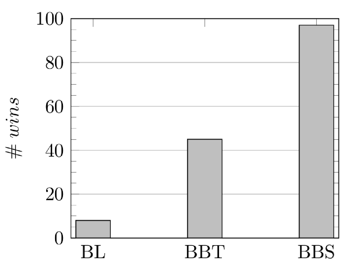
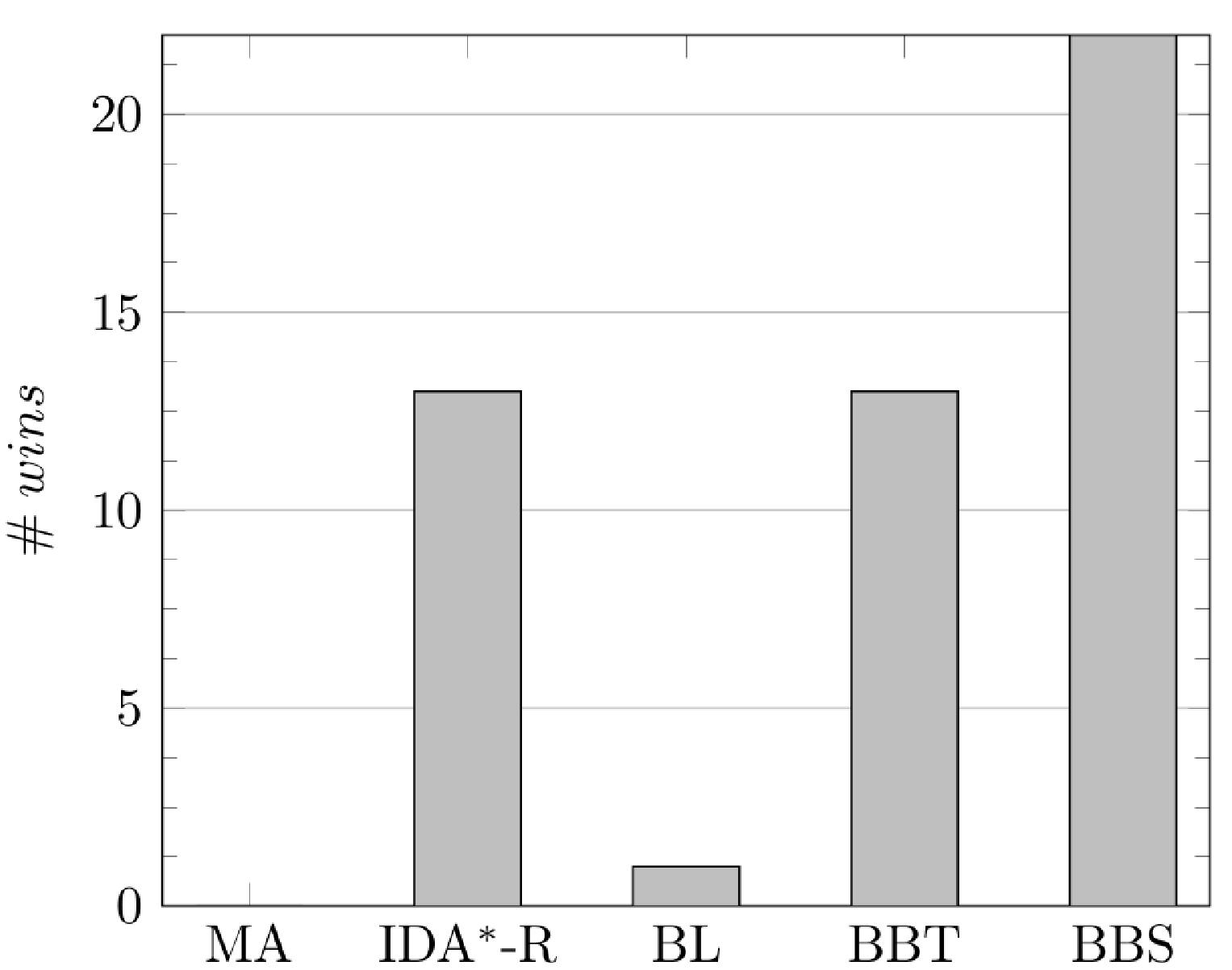
For each set of instances, we report a table with detailed results. In the tables, indicates the number of stacks, the number of available slots for each stack, the number of blocks, and #i is the number of instances of the group. Resh and Time denote the average number of reshuffles and the average computing time, respectively. Resh is in bold for the (possibly not unique) best approach. In order to evaluate the quality of the solutions provided by the heuristic algorithms, we also present, in column Opt, the average number of reshuffles obtained by the exact procedure of Tanaka and Takii 2016 within a time limit of 1800 seconds. Symbol “” in the columns indicates that the corresponding procedure runs out of time on at least one instance of the group. Symbol“” denotes that Resh = Opt. For the instances of group 1,, group 6, the tables report the solutions obtained by BBS, BBT and, in column BL, the best results provided by the algorithms that we reimplemented (Difference1, Chain, ChainF, Expected Reshuffle Index, Probe Restricted 4, the heuristic proposed in Caserta et al. 2012, Group Assignment Heuristic). Moreover, each table may include additional columns corresponding to algorithms we did not re-implement. For each algorithm we also report the machine used for the experiments. Observe that the machine we use never outperforms the ones used for the algorithms in the additional columns. For every table we also present a figure that summarizes the detailed results. Such figures report a column for each algorithm considered in the corresponding table. The height of each column measures the number of times () the associated algorithm is the best approach.
In Table 5 and Figure 4, we show the computational results obtained on the instances of group 1. Column MRIPk reports the results output by the Minimum Reshuffle Integer Program heuristic with which is the best heuristic algorithm presented in Wan et al. 2009. Since the instances are quite small, all the approaches are rather effective and both BBT and the Bounded Beam Search algorithm always provide the optimal solutions.
| MRIPka | BLb | BBTb | BBSb | |||||||||
|---|---|---|---|---|---|---|---|---|---|---|---|---|
| #i | Resh | Time | Resh | Time | Resh | Time | Resh | Time | Opt | |||
| 6 | 2 | 9 | 50 | 1.70▲ | 0.181 | 1.70▲ | 0.000 | 1.70▲ | 0.002 | 1.70▲ | 0.002 | 1.70 |
| 6 | 3 | 13 | 50 | 4.58▲ | 0.877 | 4.58▲ | 0.000 | 4.58▲ | 0.002 | 4.58▲ | 0.002 | 4.58 |
| 6 | 4 | 17 | 50 | 7.56▲ | 6.437 | 7.60 | 0.000 | 7.56▲ | 0.002 | 7.56▲ | 0.003 | 7.56 |
| 6 | 5 | 21 | 50 | 11.80 | 66.809 | 11.84 | 0.000 | 11.68▲ | 0.002 | 11.68▲ | 0.004 | 11.68 |
aIntel dual core Xeon 3GHz and 4 GB RAM
bIntel Core i7-3632QM 2.2GHz and 1 GB RAM
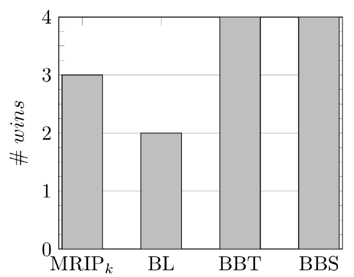
Table 6, Table 7 and Figure 5 report the computational results on the instances of group 2. Here we did not consider the results in Wu and Ting 2010 since, as confirmed us by the authors, they contain some errors. With only two exceptions, the Bounded Beam Search heuristic is always the best approach and, especially for the larger instances, outperforms all the other algorithms. Moreover, in 41 out of 100 subsets of 40 instances, the solutions provided by the Bounded Beam Search algorithm are certified to be optimal for any instance.
| BLa | BBTa | BBSa | ||||||||
|---|---|---|---|---|---|---|---|---|---|---|
| #i | Resh | Time | Resh | Time | Resh | Time | Opt | |||
| 3 | 3 | 7 | 40 | 3.30▲ | 0.000 | 3.30▲ | 0.002 | 3.30▲ | 0.002 | 3.30 |
| 3 | 4 | 9 | 40 | 5.70 | 0.000 | 5.68▲ | 0.002 | 5.68▲ | 0.002 | 5.68 |
| 3 | 5 | 11 | 40 | 8.50 | 0.000 | 8.40▲ | 0.002 | 8.40▲ | 0.002 | 8.40 |
| 3 | 6 | 13 | 40 | 12.15 | 0.000 | 11.50▲ | 0.002 | 11.50▲ | 0.002 | 11.50 |
| 3 | 7 | 15 | 40 | 15.55 | 0.000 | 15.03▲ | 0.002 | 15.03▲ | 0.003 | 15.03 |
| 3 | 8 | 17 | 40 | 19.83 | 0.000 | 18.63▲ | 0.003 | 18.63▲ | 0.004 | 18.63 |
| 3 | 9 | 19 | 40 | 25.70 | 0.000 | 23.98▲ | 0.003 | 23.98▲ | 0.013 | 23.98 |
| 3 | 10 | 21 | 40 | 31.35 | 0.000 | 28.20▲ | 0.006 | 28.20▲ | 0.042 | 28.20 |
| 3 | 11 | 23 | 40 | 37.93 | 0.000 | 32.70▲ | 0.011 | 32.75 | 0.070 | 32.70 |
| 3 | 12 | 25 | 40 | 42.38 | 0.000 | 36.43▲ | 0.035 | 36.43▲ | 0.090 | 36.43 |
| 4 | 3 | 10 | 40 | 4.85▲ | 0.000 | 4.85▲ | 0.002 | 4.85▲ | 0.002 | 4.85 |
| 4 | 4 | 13 | 40 | 8.53 | 0.000 | 8.43▲ | 0.002 | 8.43▲ | 0.002 | 8.43 |
| 4 | 5 | 16 | 40 | 12.55 | 0.000 | 12.25▲ | 0.002 | 12.25▲ | 0.003 | 12.25 |
| 4 | 6 | 19 | 40 | 16.35 | 0.000 | 15.63▲ | 0.002 | 15.63▲ | 0.004 | 15.63 |
| 4 | 7 | 22 | 40 | 24.23 | 0.000 | 22.60▲ | 0.003 | 22.60▲ | 0.023 | 22.60 |
| 4 | 8 | 25 | 40 | 30.65 | 0.000 | 27.70▲ | 0.006 | 27.70▲ | 0.053 | 27.70 |
| 4 | 9 | 28 | 40 | 36.20 | 0.000 | 32.43▲ | 0.040 | 32.43▲ | 0.168 | 32.43 |
| 4 | 10 | 31 | 40 | 45.33 | 0.000 | 40.35 | 0.284 | 40.15 | 0.287 | 40.05 |
| 4 | 11 | 34 | 40 | 53.88 | 0.001 | 46.10 | 0.482 | 45.73 | 0.383 | 45.60 |
| 4 | 12 | 37 | 40 | 64.90 | 0.001 | 55.55 | 0.823 | 54.38 | 0.612 | |
| 5 | 3 | 13 | 40 | 5.75▲ | 0.000 | 5.75▲ | 0.002 | 5.75▲ | 0.002 | 5.75 |
| 5 | 4 | 17 | 40 | 11.10 | 0.000 | 10.98▲ | 0.002 | 10.98▲ | 0.003 | 10.98 |
| 5 | 5 | 21 | 40 | 16.10 | 0.000 | 15.58▲ | 0.002 | 15.58▲ | 0.005 | 15.58 |
| 5 | 6 | 25 | 40 | 22.10 | 0.000 | 21.05▲ | 0.003 | 21.05▲ | 0.028 | 21.05 |
| 5 | 7 | 29 | 40 | 30.00 | 0.000 | 27.53▲ | 0.019 | 27.55 | 0.101 | 27.53 |
| 5 | 8 | 33 | 40 | 39.55 | 0.000 | 35.85 | 0.187 | 35.83 | 0.302 | 35.80 |
| 5 | 9 | 37 | 40 | 47.18 | 0.000 | 41.48 | 0.293 | 41.40 | 0.404 | 41.25 |
| 5 | 10 | 41 | 40 | 57.33 | 0.001 | 51.13 | 0.826 | 50.18 | 0.422 | |
| 5 | 11 | 45 | 40 | 68.35 | 0.001 | 60.50 | 1.079 | 57.78 | 0.606 | |
| 5 | 12 | 49 | 40 | 81.33 | 0.000 | 74.53 | 1.242 | 68.15 | 0.807 | |
| 6 | 3 | 16 | 40 | 7.65▲ | 0.000 | 7.65▲ | 0.002 | 7.65▲ | 0.004 | 7.65 |
| 6 | 4 | 21 | 40 | 12.20 | 0.000 | 12.03▲ | 0.002 | 12.03▲ | 0.003 | 12.03 |
| 6 | 5 | 26 | 40 | 20.08 | 0.000 | 19.33▲ | 0.003 | 19.33▲ | 0.012 | 19.33 |
| 6 | 6 | 31 | 40 | 27.58 | 0.000 | 25.98▲ | 0.007 | 25.98▲ | 0.071 | 25.98 |
| 6 | 7 | 36 | 40 | 37.90 | 0.000 | 34.43 | 0.182 | 34.45 | 0.305 | 34.40 |
| 6 | 8 | 41 | 40 | 47.13 | 0.001 | 42.50 | 0.424 | 42.25 | 0.295 | 42.10 |
| 6 | 9 | 46 | 40 | 58.45 | 0.001 | 52.93 | 0.986 | 51.15 | 0.516 | |
| 6 | 10 | 51 | 40 | 70.43 | 0.002 | 64.58 | 1.197 | 61.50 | 0.793 | |
| 6 | 11 | 56 | 40 | 84.18 | 0.003 | 76.43 | 1.273 | 71.35 | 0.972 | |
| 6 | 12 | 61 | 40 | 99.75 | 0.000 | 93.08 | 1.271 | 82.73 | 0.738 | |
| 7 | 3 | 19 | 40 | 8.95▲ | 0.000 | 8.95▲ | 0.002 | 8.95▲ | 0.003 | 8.95 |
| 7 | 4 | 25 | 40 | 15.68 | 0.000 | 15.48▲ | 0.002 | 15.48▲ | 0.004 | 15.48 |
| 7 | 5 | 31 | 40 | 22.08 | 0.000 | 21.35▲ | 0.004 | 21.35▲ | 0.023 | 21.35 |
| 7 | 6 | 37 | 40 | 32.58 | 0.000 | 30.75▲ | 0.031 | 30.75▲ | 0.185 | 30.75 |
| 7 | 7 | 43 | 40 | 42.33 | 0.001 | 39.05 | 0.384 | 39.00 | 0.327 | 38.95 |
| 7 | 8 | 49 | 40 | 54.03 | 0.001 | 50.20 | 0.912 | 48.85 | 0.560 | |
| 7 | 9 | 55 | 40 | 69.00 | 0.002 | 63.58 | 1.221 | 61.03 | 0.853 | |
| 7 | 10 | 61 | 40 | 81.05 | 0.003 | 75.95 | 1.230 | 70.15 | 0.607 | |
| 7 | 11 | 67 | 40 | 97.33 | 0.000 | 91.98 | 1.259 | 83.58 | 0.849 | |
| 7 | 12 | 73 | 40 | 115.88 | 0.008 | 110.63 | 1.403 | 98.05 | 0.977 | |
a CPU Intel Core i7-3632QM 2.20GHz with 1.0 GB RAM
| BLa | BBTa | BBSa | ||||||||
|---|---|---|---|---|---|---|---|---|---|---|
| #i | Resh | Time | Resh | Time | Resh | Time | Opt | |||
| 8 | 3 | 22 | 40 | 9.73▲ | 0.000 | 9.73▲ | 0.002 | 9.73▲ | 0.004 | 9.73 |
| 8 | 4 | 29 | 40 | 18.18 | 0.000 | 17.95▲ | 0.003 | 17.95▲ | 0.008 | 17.95 |
| 8 | 5 | 36 | 40 | 26.00 | 0.000 | 25.40▲ | 0.005 | 25.40▲ | 0.047 | 25.40 |
| 8 | 6 | 43 | 40 | 38.20 | 0.000 | 35.75 | 0.173 | 35.70 | 0.182 | 35.68 |
| 8 | 7 | 50 | 40 | 48.90 | 0.001 | 44.90 | 0.480 | 44.63 | 0.451 | 44.48 |
| 8 | 8 | 57 | 40 | 62.08 | 0.002 | 57.53 | 1.125 | 55.70 | 0.738 | |
| 8 | 9 | 64 | 40 | 77.00 | 0.003 | 72.23 | 1.218 | 68.45 | 0.633 | |
| 8 | 10 | 71 | 40 | 94.60 | 0.000 | 87.83 | 1.244 | 80.90 | 0.882 | |
| 8 | 11 | 78 | 40 | 114.53 | 0.000 | 109.93 | 1.367 | 99.10 | 0.973 | |
| 8 | 12 | 85 | 40 | 136.63 | 0.000 | 131.85 | 1.476 | 113.50 | 0.984 | |
| 9 | 3 | 25 | 40 | 11.45▲ | 0.000 | 11.45▲ | 0.002 | 11.45▲ | 0.004 | 11.45 |
| 9 | 4 | 33 | 40 | 19.53 | 0.000 | 19.15▲ | 0.003 | 19.15▲ | 0.009 | 19.15 |
| 9 | 5 | 41 | 40 | 29.40 | 0.000 | 28.65▲ | 0.014 | 28.65▲ | 0.048 | 28.65 |
| 9 | 6 | 49 | 40 | 42.43 | 0.001 | 39.80 | 0.292 | 39.70 | 0.310 | 39.63 |
| 9 | 7 | 57 | 40 | 55.18 | 0.001 | 51.65 | 0.872 | 50.73 | 0.645 | |
| 9 | 8 | 65 | 40 | 71.33 | 0.003 | 67.70 | 1.185 | 64.48 | 0.603 | |
| 9 | 9 | 73 | 40 | 89.45 | 0.000 | 84.23 | 1.274 | 78.75 | 0.849 | |
| 9 | 10 | 81 | 40 | 108.05 | 0.000 | 103.20 | 1.408 | 93.80 | 0.811 | |
| 9 | 11 | 89 | 40 | 126.45 | 0.000 | 122.63 | 1.392 | 108.75 | 0.995 | |
| 9 | 12 | 97 | 40 | 149.58 | 0.000 | 146.25 | 1.515 | 128.30 | 1.008 | |
| 10 | 3 | 28 | 40 | 11.88▲ | 0.000 | 11.88▲ | 0.002 | 11.88▲ | 0.005 | 11.88 |
| 10 | 4 | 37 | 40 | 22.75 | 0.000 | 22.35▲ | 0.003 | 22.35▲ | 0.009 | 22.35 |
| 10 | 5 | 46 | 40 | 32.95 | 0.000 | 31.73 | 0.091 | 31.73 | 0.115 | 31.70 |
| 10 | 6 | 55 | 40 | 46.03 | 0.001 | 43.93 | 0.448 | 43.58 | 0.344 | 43.55 |
| 10 | 7 | 64 | 40 | 62.28 | 0.002 | 58.08 | 1.053 | 56.38 | 0.482 | |
| 10 | 8 | 73 | 40 | 77.25 | 0.004 | 72.75 | 1.375 | 69.28 | 0.730 | |
| 10 | 9 | 82 | 40 | 97.18 | 0.007 | 93.00 | 1.493 | 86.43 | 0.782 | |
| 10 | 10 | 91 | 40 | 117.65 | 0.012 | 114.10 | 1.501 | 102.40 | 0.978 | |
| 10 | 11 | 100 | 40 | 140.25 | 0.000 | 138.63 | 1.502 | 121.55 | 0.727 | |
| 10 | 12 | 109 | 40 | 160.08 | 0.000 | 158.08 | 1.470 | 137.68 | 0.896 | |
| 11 | 3 | 31 | 40 | 14.23 | 0.000 | 14.13▲ | 0.002 | 14.13▲ | 0.006 | 14.13 |
| 11 | 4 | 41 | 40 | 23.90 | 0.000 | 23.43▲ | 0.004 | 23.43▲ | 0.012 | 23.43 |
| 11 | 5 | 51 | 40 | 36.13 | 0.000 | 35.05▲ | 0.044 | 35.05▲ | 0.135 | 35.05 |
| 11 | 6 | 61 | 40 | 50.30 | 0.001 | 48.00 | 0.783 | 47.13 | 0.329 | |
| 11 | 7 | 71 | 40 | 68.23 | 0.003 | 64.75 | 1.260 | 62.33 | 0.584 | |
| 11 | 8 | 81 | 40 | 87.45 | 0.005 | 83.95 | 1.438 | 79.13 | 0.601 | |
| 11 | 9 | 91 | 40 | 110.15 | 0.010 | 105.75 | 1.475 | 96.75 | 0.918 | |
| 11 | 10 | 101 | 40 | 130.95 | 0.016 | 127.78 | 1.506 | 115.15 | 0.639 | |
| 11 | 11 | 111 | 40 | 153.33 | 0.027 | 150.85 | 1.367 | 133.03 | 0.891 | |
| 11 | 12 | 121 | 40 | 180.15 | 0.000 | 179.15 | 1.516 | 156.05 | 0.621 | |
| 12 | 3 | 34 | 40 | 14.95 | 0.000 | 14.90▲ | 0.002 | 14.90▲ | 0.006 | 14.90 |
| 12 | 4 | 45 | 40 | 27.15 | 0.000 | 26.80▲ | 0.004 | 26.80▲ | 0.023 | 26.80 |
| 12 | 5 | 56 | 40 | 40.48 | 0.001 | 39.10 | 0.309 | 39.05 | 0.282 | 39.00 |
| 12 | 6 | 67 | 40 | 55.40 | 0.001 | 52.43 | 0.748 | 51.75 | 0.360 | |
| 12 | 7 | 78 | 40 | 74.75 | 0.003 | 71.60 | 1.446 | 69.15 | 0.809 | |
| 12 | 8 | 89 | 40 | 95.65 | 0.007 | 92.18 | 1.500 | 86.45 | 0.753 | |
| 12 | 9 | 100 | 40 | 117.63 | 0.013 | 112.85 | 1.548 | 104.25 | 0.591 | |
| 12 | 10 | 111 | 40 | 137.40 | 0.000 | 135.63 | 1.524 | 121.25 | 0.812 | |
| 12 | 11 | 122 | 40 | 170.60 | 0.000 | 169.35 | 1.506 | 147.55 | 0.580 | |
| 12 | 12 | 133 | 40 | 198.80 | 0.000 | 198.10 | 1.685 | 171.68 | 0.849 | |
a CPU Intel Core i7-3632QM 2.20GHz with 1.0 GB RAM
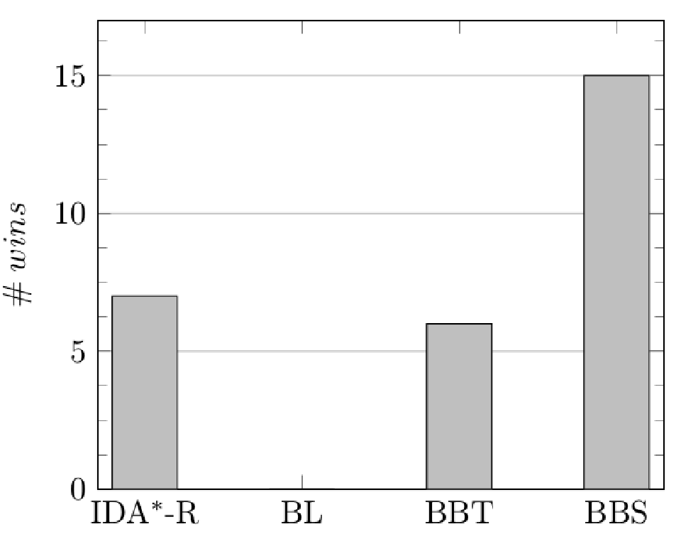
In Table 8 and Figure 6 the computational results obtained on the instances of group 3 are shown. Column id indicates if the instances are Random (R) or Upside down (U), while column b reports the number of bays. Symbol “-” in Columns Resh and Time for the iterative deepening A* restricted by Zhu et al. 2012 (IDA∗-R) means that the value of the solution and the computing time are not available in the literature. For most of the instances, the Bounded Beam Search approach produces the best results. Observe that the R instances turn out to be harder to solve than the U ones.
| 3PHa | IDA∗-Rb | BLc | BBTc | BBSc | ||||||||||||
|---|---|---|---|---|---|---|---|---|---|---|---|---|---|---|---|---|
| id | #i | Resh | Time | Resh | Time | Resh | Time | Resh | Time | Resh | Time | Opt | ||||
| R | 1 | 16 | 6 | 70 | 5 | 55.40 | 8204.32 | 40.00 | - | 39.80 | 0.00 | 40.00 | 0.59 | 39.60 | 0.60 | |
| R | 1 | 16 | 8 | 90 | 5 | 101.40 | 13353.36 | 63.00 | - | 63.00 | 0.01 | 63.40 | 2.63 | 61.40 | 0.75 | |
| R | 2 | 32 | 6 | 140 | 5 | 90.20 | 21579.55 | - | - | 71.80 | 0.01 | 71.80 | 0.45 | 71.60 | 0.11 | |
| R | 2 | 32 | 8 | 190 | 5 | 177.80 | 21527.71 | - | - | 125.40 | 0.00 | 125.40 | 9.16 | 124.00 | 0.80 | |
| R | 4 | 64 | 6 | 280 | 5 | 174.20 | 21522.11 | - | - | 151.60 | 0.09 | 152.60 | 71.65 | 152.40 | 0.60 | |
| R | 4 | 64 | 8 | 380 | 5 | 389.20 | 21231.08 | - | - | 242.80 | 0.00 | 245.40 | 9.39 | 243.60 | 1.00 | |
| R | 6 | 96 | 6 | 430 | 5 | 279.8 | 21358.80 | - | - | 226.60 | 0.00 | 226.60 | 6.45 | 226.60 | 0.40 | |
| R | 6 | 96 | 8 | 570 | 5 | 672.00 | 20874.03 | - | - | 352.40 | 0.00 | 353.60 | 116.88 | 352.00 | 0.60 | |
| R | 8 | 128 | 6 | 570 | 5 | 375.40 | 21200.97 | - | - | 305.60▲ | 0.00 | 305.60▲ | 0.16 | 305.60▲ | 0.00 | 305.60 |
| R | 10 | 160 | 6 | 720 | 5 | 449.20 | 20844.76 | - | - | 372.60 | 0.22 | 372.80 | 7.20 | 372.80 | 0.21 | |
| U | 1 | 16 | 6 | 70 | 2 | 57.50 | 14284.86 | 56.50▲ | - | 56.50▲ | 0.00 | 56.50▲ | 0.00 | 56.50▲ | 0.00 | 56.50 |
| U | 1 | 16 | 8 | 90 | 2 | 87.50 | 14804.06 | 77.00▲ | - | 77.00▲ | 0.00 | 77.00▲ | 0.00 | 77.00▲ | 0.00 | 77.00 |
| U | 2 | 32 | 6 | 140 | 2 | 117.00 | 21543.79 | - | - | 109.00▲ | 0.00 | 109.00▲ | 0.04 | 109.00▲ | 0.00 | 109.00 |
| U | 2 | 32 | 8 | 190 | 2 | 210.50 | 21371.03 | - | - | 160.00▲ | 0.01 | 160.00▲ | 0.06 | 160.00▲ | 0.00 | 160.00 |
| U | 4 | 64 | 6 | 280 | 2 | 227.50 | 21321.99 | - | - | 216.50▲ | 0.00 | 216.50▲ | 0.07 | 216.50▲ | 0.00 | 216.50 |
| U | 4 | 64 | 8 | 380 | 2 | 420.00 | 20890.37 | - | - | 318.50▲ | 0.00 | 318.50▲ | 0.07 | 318.50▲ | 0.00 | 318.50 |
| U | 6 | 96 | 6 | 430 | 2 | 363.00 | 20929.72 | - | - | 334.00▲ | 0.00 | 334.00▲ | 0.17 | 334.00▲ | 0.00 | 334.00 |
| U | 6 | 96 | 8 | 570 | 2 | 664.00 | 20066.65 | - | - | 476.00▲ | 0.00 | 476.00▲ | 0.21 | 476.00▲ | 0.00 | 476.00 |
| U | 8 | 128 | 6 | 570 | 2 | 474.00 | 20504.17 | - | - | 443.50▲ | 0.00 | 443.50▲ | 0.26 | 443.50▲ | 0.01 | 443.50 |
| U | 10 | 160 | 6 | 720 | 2 | 625.00 | 19722.45 | - | - | 561.00▲ | 0.00 | 561.00▲ | 0.32 | 561.00▲ | 0.01 | 561.00 |
aCore 2 Duo E8500 3.42GHz and 3.46 GB RAM
bIntel Core i7-920 2.66GHz and 12 GB RAM
cIntel Core i7-3632QM 2.2GHz and 1 GB RAM
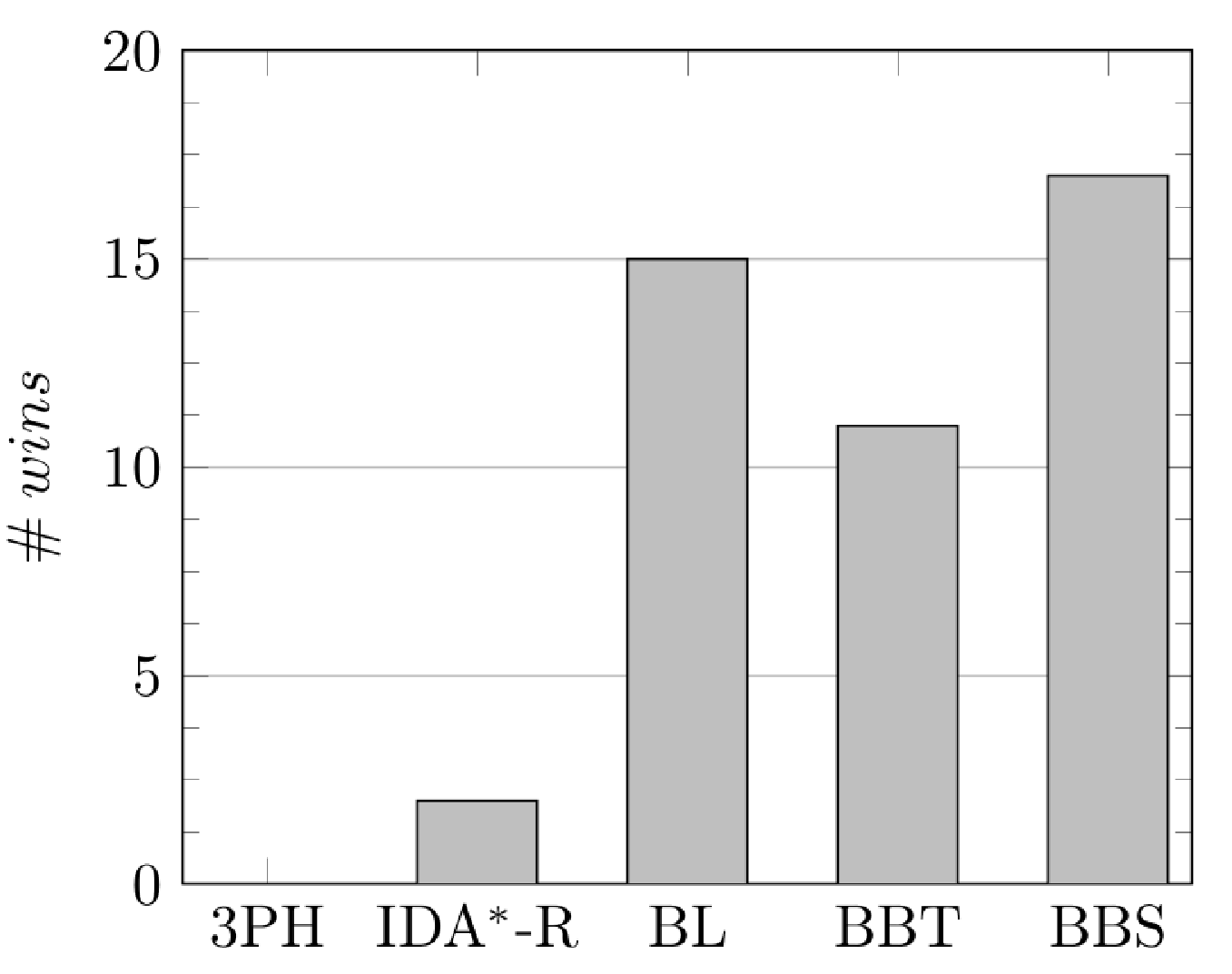
Table 9 and Figure 7 report the computational results on the instances of group 4. Here, we did not consider the results in Caserta et al. 2011 since, as reported in Zhu et al. 2012, they contain some errors. Symbol “-” in Columns Resh and Time for the Matrix-Algorithm by Caserta et al. 2009 (MA) and the iterative deepening A* restricted by Zhu et al. 2012 (IDA∗-R) means that the value of the solution and the computing time are not available in the literature. Here, the Bounded Beam Search method is always the best approach and in most of the cases it finds the optimal solution.
| MAa | IDA∗-Rb | BLc | BBTc | BBSc | ||||||||||
|---|---|---|---|---|---|---|---|---|---|---|---|---|---|---|
| #i | Resh | Time | Resh | Time | Resh | Time | Resh | Time | Resh | Time | Opt | |||
| 3 | 5 | 9 | 40 | - | - | 5.000▲ | - | 5.025 | 0.000 | 5.000▲ | 0.003 | 5.000▲ | 0.002 | 5.000 |
| 3 | 6 | 12 | 40 | - | - | 6.175▲ | - | 6.225 | 0.000 | 6.175▲ | 0.002 | 6.175▲ | 0.002 | 6.175 |
| 3 | 7 | 15 | 40 | - | - | 7.025▲ | - | 7.025▲ | 0.000 | 7.025▲ | 0.002 | 7.025▲ | 0.003 | 7.025 |
| 3 | 8 | 18 | 40 | - | - | 8.400▲ | - | 8.425 | 0.000 | 8.400▲ | 0.002 | 8.400▲ | 0.004 | 8.400 |
| 3 | 9 | 21 | 40 | - | - | 9.275▲ | - | 9.325 | 0.000 | 9.275▲ | 0.002 | 9.275▲ | 0.004 | 9.275 |
| 3 | 10 | 24 | 40 | - | - | 10.650▲ | - | 10.700 | 0.000 | 10.650▲ | 0.002 | 10.650▲ | 0.005 | 10.650 |
| 4 | 6 | 16 | 40 | - | - | 10.200▲ | - | 10.425 | 0.000 | 10.200▲ | 0.002 | 10.200▲ | 0.003 | 10.200 |
| 4 | 7 | 20 | 40 | - | - | 12.950▲ | - | 13.175 | 0.000 | 12.950▲ | 0.002 | 12.950▲ | 0.010 | 12.950 |
| 4 | 8 | 24 | 40 | - | - | 14.025▲ | - | 14.300 | 0.000 | 14.025▲ | 0.003 | 14.025▲ | 0.033 | 14.025 |
| 4 | 9 | 28 | 40 | - | - | 16.125▲ | - | 16.525 | 0.000 | 16.125▲ | 0.003 | 16.125▲ | 0.046 | 16.125 |
| 5 | 6 | 20 | 40 | - | - | 15.425▲ | - | 16.275 | 0.000 | 15.425▲ | 0.003 | 15.425▲ | 0.010 | 15.425 |
| 5 | 7 | 25 | 40 | - | - | 18.850▲ | - | 19.850 | 0.000 | 18.850▲ | 0.005 | 18.850▲ | 0.065 | 18.850 |
| 5 | 8 | 30 | 40 | - | - | 22.075▲ | - | 23.525 | 0.000 | 22.075▲ | 0.041 | 22.075▲ | 0.172 | 22.075 |
| 5 | 9 | 35 | 40 | - | - | 24.300 | - | 25.375 | 0.000 | 24.400 | 0.187 | 24.250▲ | 0.318 | 24.250 |
| 5 | 10 | 40 | 40 | - | - | 27.850 | - | 28.650 | 0.000 | 28.000 | 0.316 | 27.750 | 0.371 | 27.700 |
| 5 | 11 | 45 | 40 | - | - | 30.675 | - | 31.350 | 0.001 | 30.900 | 0.513 | 30.525 | 0.599 | 30.450 |
| 5 | 12 | 50 | 40 | - | - | 33.625 | - | 34.300 | 0.001 | 34.350 | 0.642 | 33.325 | 0.667 | |
| 6 | 8 | 36 | 40 | 31.8 | 0.38 | 31.075 | - | 34.050 | 0.001 | 31.050 | 0.447 | 30.925 | 0.566 | |
| 6 | 12 | 60 | 40 | 47.6 | 0.65 | 47.200 | - | 48.650 | 0.003 | 48.100 | 1.211 | 46.000 | 0.836 | |
| 10 | 8 | 60 | 40 | 82.9 | 0.93 | 84.975 | - | 91.725 | 0.000 | 85.700 | 1.314 | 77.300 | 0.788 | |
| 10 | 12 | 100 | 40 | 121.3 | 1.57 | 126.325 | - | 128.350 | 0.000 | 132.025 | 1.927 | 112.475 | 0.917 | |
| 100 | 102 | 10000 | 40 | - | - | - | - | 63358.246 | 0.190 | 62413.277 | 1.111 | |||
aPentium IV and 512 MB RAM
bIntel Core i7-920 2.66GHz and 12 GB RAM
cIntel Core i7-3632QM 2.2GHz and 1 GB RAM
In Table 10 and Figure 8, the computational results obtained on the instances of group 5 are shown. Column type denotes if the instances are balanced (b) or unbalanced (u) and column d reports the storage density. For the sake of conciseness, in the table we report only the rows where at least one between BBT and the Bounded Beam Search methods does not find the optimal solution. However, the results on all the instances are considered in the figure. According to these results, the two procedures present similar behaviors and both outperform BL.
| BL | BBT | BBS | ||||||||||
|---|---|---|---|---|---|---|---|---|---|---|---|---|
| type | delta | #i | Resh | Time | Resh | Time | Resh | Time | Opt | |||
| b | 6 | 7 | 29 | 70% | 40 | 17.580 | 0.00 | 17.180▲ | 0.01 | 17.200 | 0.12 | 17.180 |
| b | 7 | 6 | 31 | 75% | 40 | 24.550 | 0.00 | 23.150▲ | 0.02 | 23.180 | 0.18 | 23.150 |
| b | 7 | 7 | 31 | 65% | 40 | 20.030 | 0.00 | 19.480 | 0.04 | 19.430▲ | 0.13 | 19.430 |
| b | 7 | 7 | 36 | 75% | 40 | 27.280 | 0.00 | 25.900 | 0.12 | 25.900 | 0.42 | 25.850 |
| u | 6 | 7 | 31 | 75% | 40 | 20.350 | 0.00 | 19.700▲ | 0.02 | 19.730 | 0.06 | 19.700 |
| u | 7 | 5 | 21 | 60% | 40 | 15.300 | 0.00 | 14.730▲ | 0.00 | 14.750 | 0.02 | 14.730 |
| u | 7 | 7 | 36 | 75% | 40 | 27.700 | 0.00 | 26.350 | 0.16 | 26.330 | 0.38 | 26.300 |
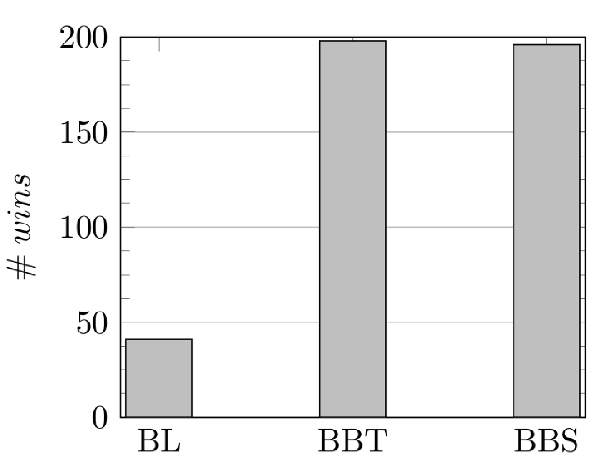
We present the computational results on the instances of group 6 in Table 11 and Figure 9. In the table, according to the results in the literature, we report total reshuffles and times instead of the average values. Also in this case, the Bounded Beam Search heuristic outperforms all the other approaches.
| IDA∗-Ra | BLb | BBTb | BBSb | ||||||||
|---|---|---|---|---|---|---|---|---|---|---|---|
| #i | Resh | Time | Resh | Time | Resh | Time | Resh | Time | Opt | ||
| 6-10 | 3 | 1500 | 13592▲ | 0.00 | 13603 | 0.00 | 13592▲ | 2.94 | 13592▲ | 6.01 | 13592 |
| 6-10 | 4 | 2000 | 33095▲ | 0.12 | 33535 | 0.10 | 33095▲ | 6.10 | 33095▲ | 13.30 | 33095 |
| 6 | 5 | 500 | 9503▲ | 0.05 | 9763 | 0.06 | 9503▲ | 1.37 | 9503▲ | 4.92 | 9503 |
| 7 | 5 | 500 | 11259▲ | 0.16 | 11634 | 0.06 | 11259▲ | 1.78 | 11259▲ | 13.24 | 11259 |
| 8 | 5 | 500 | 12864 | 1.24 | 13232 | 0.08 | 12864 | 4.80 | 12863▲ | 26.68 | 12863 |
| 9 | 5 | 500 | 14158 | 2.74 | 14608 | 0.11 | 14158 | 10.81 | 14158 | 31.44 | 14156 |
| 10 | 5 | 500 | 15727 | 6.91 | 16214 | 0.14 | 15728 | 21.69 | 15731 | 51.42 | 15726 |
| 6 | 6 | 600 | 16175▲ | 4.56 | 17084 | 0.11 | 16175▲ | 5.06 | 16176 | 38.20 | 16175 |
| 7 | 6 | 600 | 18607 | 10.72 | 19615 | 0.17 | 18606 | 21.44 | 18603 | 72.12 | 18601 |
| 8 | 6 | 600 | 21221 | 18.90 | 22385 | 0.25 | 21211 | 61.66 | 21195 | 96.70 | 21187 |
| 9 | 6 | 600 | 23790 | 36.72 | 25121 | 0.35 | 23793 | 158.69 | 23726 | 167.90 | |
| 10 | 6 | 600 | 26125 | 46.83 | 27518 | 0.47 | 26149 | 238.96 | 26025 | 238.13 | |
| 6 | 7 | 700 | 24860 | 41.07 | 26694 | 0.25 | 24831 | 66.55 | 24827 | 136.22 | 24813 |
| 7 | 7 | 700 | 28930 | 78.73 | 31124 | 0.41 | 28884 | 192.74 | 28835 | 192.75 | 28771 |
| 8 | 7 | 700 | 32782 | 102.69 | 35153 | 0.64 | 32701 | 404.96 | 32454 | 301.74 | |
| 9 | 7 | 700 | 37014 | 116.18 | 39483 | 0.90 | 37064 | 604.61 | 36494 | 349.37 | |
| 10 | 7 | 700 | 40896 | 129.75 | 43429 | 1.27 | 41053 | 732.33 | 40132 | 307.79 | |
aPentium-IV 3.0 GHz and 1.0 GB RAM
b CPU Intel Core i7-3632QM 2.20GHz and 1.0 GB RAM
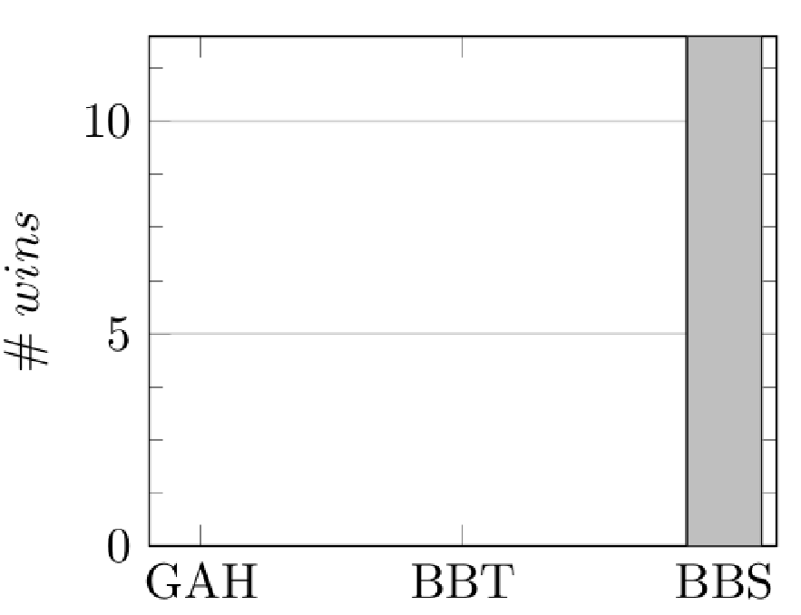
Finally, in Table 12 and Figure 10, we report the results on the instances of lbri. Here, BBT can not find feasible solutions within the time limit on all the subsets of instances. The Bounded Beam Search heuristic is again the best approach.
Reviewing the whole computational experience, the Bounded Beam Search procedure presents the best results on almost all instances in the dataset. In particular, in the sets for which all the instances are solved to optimality, the Bounded Beam Search heuristic finds such an optimum in more than 70% of the cases.
We think that such good performances are related to the combined use of upper and lower bound in the selection of the most promising descendants of each node, in particular for breaking ties in the evaluation. Table 4 emphasizes the dependency of the overall algorithm from the choice of an appropriate upper bound.
The second best algorithm is the one of Tanaka and Takii 2016, when used as a heuristic by fixing a time limit of one second (BBT). Nevertheless, it becomes impractical for large instances although the exact variant is extremely efficient for the small ones.
| BLa | BBTa | BBSa | |||||||
|---|---|---|---|---|---|---|---|---|---|
| #i | Resh | Time | Resh | Time | Resh | Time | |||
| 50 | 4 | [196,199] | 400 | 99.755 | 0.004 | 98.803 | 0.111 | ||
| 50 | 7 | [343,349] | 700 | 271.676 | 0.000 | 261.684 | 1.003 | ||
| 50 | 10 | [490,499] | 1000 | 515.823 | 0.001 | 499.245 | 1.004 | ||
| 100 | 4 | [396,399] | 400 | 196.313 | 0.024 | 195.145 | 0.379 | ||
| 100 | 7 | [693,699] | 700 | 512.937 | 0.001 | 505.373 | 1.004 | ||
| 100 | 10 | [990,999] | 1000 | 964.140 | 0.002 | 952.621 | 1.005 | ||
| 500 | 4 | [1996,1999] | 400 | 964.168 | 0.116 | 963.383 | 0.843 | ||
| 500 | 7 | [3493,3499] | 700 | 2338.576 | 0.008 | 2331.293 | 1.013 | ||
| 500 | 10 | [4990,4999] | 1000 | 4277.015 | 0.014 | 4248.174 | 1.016 | ||
| 1000 | 4 | [3996,3999] | 400 | 1922.303 | 0.014 | 1921.778 | 0.919 | ||
| 1000 | 7 | [6993,6999] | 700 | 4561.887 | 0.029 | 4556.585 | 1.030 | ||
| 1000 | 10 | [9990,9999] | 1000 | 8135.950 | 0.050 | 8109.102 | 1.037 | ||
a CPU Intel Core i7-3632QM 2.20GHz and 1.0 GB RAM
9 Conclusions
In this paper we considered the Block Relocation Problem, which has relevant practical applications in the container logistics. The problem is difficult both in theory and in practice and even the most effective exact approaches fail to solve instances with size far away from the real ones. In this paper we introduced a new lower bound and a new beam search heuristic for the problem. The lower bound dominates most of the existing ones and it can be calculated by a polynomial time algorithm. The beam search heuristic includes such procedure in order to reduce the search space and select the most promising nodes. The results show that the proposed heuristic is very effective and outperforms all the other approaches on most of the considered instances. The algorithm is also tested on a new set of real-size instances, lbri, introduced here for the first time.
Acknowledgements
The authors have been partially supported by Ministry of Instruction University and Research (MIUR) with the program PRIN 2015, project “SPORT - Smart PORt Terminals”, code 2015XAPRKF; project “Nonlinear and Combinatorial Aspects of Complex Networks”, code 2015B5F27W; project “Scheduling cuts: new optimization models and algorithms for cutting, packing and nesting in manufacturing processes”, code 20153TXRX9; the CONtainer TRAnshipment STation (CONTRAST) 2013 project, code FILAS-CR-2011-1315.
References
- Bacci [2017] T. Bacci. Bacci website, 2017. URL http://www.iasi.cnr.it/˜tbacci/.
- Bacci et al. [2017] T. Bacci, S. Mattia, and P. Ventura. Some complexity results for the minimum blocking items problem. In Optimization and Decision Science (ODS 2017): Methodologies and Applications, volume 217 of Springer Proceedings in Mathematics and Statistics, pages 475–483, 2017.
- Bacci et al. [2018] T. Bacci, S. Mattia, and P. Ventura. A new lower bound for the Block Relocation Problem. In International Conference on Computation and Logistics – ICCL 2018, Lecture Notes In Computer Science, 11184, pp. 168–174, 2018.
- Bonomo et al. [2011] F. Bonomo, S. Mattia, and G. Oriolo. Bounded coloring of co-comparability graphs and the pickup and delivery tour combination problem. Theoretical Computer Science, 412(45):6261 – 6268, 2011.
- Carlo et al. [2014] H.J. Carlo, I.F.A. Vis, and K.J. Roodbergen. Storage yard operations in container terminals: Literature overview, trends, and research directions. European Journal of Operational Research, 235(2):412 – 430, 2014.
- Caserta et al. [2009] M. Caserta, S. Schwarze, and S. Voß. A new binary description of the blocks relocation problem and benefits in a look ahead heuristic. Proceedings of the EvoCOP 2009, pages 37–48, 2009.
- Caserta et al. [2011] M. Caserta, S. Voß, and M. Sniedovich. Applying the corridor method to a blocks relocation problem. OR Spectrum, 33(4):915–929, 2011.
- Caserta et al. [2012] M. Caserta, S. Schwarze, and S. Voß. A mathematical formulation and complexity considerations for the blocks relocation problem. European Journal of Operational Research, 219:96–104, 2012.
- Forster and Bortfeldt [2012] F. Forster and A. Bortfeldt. A tree search procedure for the container relocation problem. Computers & Operations Research, 39:299–309, 2012.
- Günter and Kim [2005] H. O. Günter and K. H. Kim. Container Terminals and Automated Transport Systems. Springer Berlin Heidelberg, 2005.
- Hottung and Tierney [2016] A. Hottung and K. Tierney. A biased random-key genetic algorithm for the container pre-marshalling problem. Computers & Operations Research, 75:83 – 102, 2016.
- Izquierdo et al. [2014] C. E. Izquierdo, B. M. Batista, and J. M. M. Vega. A domain-specific knowledge-based heuristic for the blocks relocation problem. Advanced Engineering Informatics 28, 28:327–343, 2014.
- Izquierdo et al. [2015] C. E. Izquierdo, B. M. Batista, and J. M. M. Vega. An exact approach for the blocks relocation problem. Expert Systems with Applications, 42:6408–6422, 2015.
- Jansen [2003] K. Jansen. The mutual exclusion scheduling problem for permutation and comparability graphs. Information and Computation, 180:71–81, 2003.
- Jovanovic and Voß [2014] R. Jovanovic and S. Voß. A chain heuristic for the blocks relocation problem. Computers & Industrial Engineering, 75:79 – 86, 2014.
- Jovanovic et al. [2017] R. Jovanovic, M. Tuba, and S. Voß. A multi-heuristic approach for solving the pre-marshalling problem. Central European Journal of Operations Research, 25(1):1–28, 2017.
- Kim and Hong [2006] K. H. Kim and G. P. Hong. A heuristic rule for relocating blocks. Computers & Operations Research, 33:940–954, 2006.
- Ku and Arthanari [2016a] D. Ku and T. S. Arthanari. Container relocation problem with time windows for container departure. European Journal of Operational Research, 252(3):1031 – 1039, 2016a.
- Ku and Arthanari [2016b] D. Ku and T.S. Arthanari. On the abstraction method for the container relocation problem. Computers & Operations Research, 68(Supplement C):110 – 122, 2016b.
- Lee and Hsu [2007] Y. Lee and N. Y. Hsu. An optimization model for the container pre-marshalling problem. Computers & Operations Research, 34(11):3295 – 3313, 2007.
- Lee and Lee [2010] Y. Lee and Y. L. Lee. A heuristic for retrieving containers from a yard. Computers & Operations Research, 47:1139–1147, 2010.
- Lehnfeld and Knust [2014] J. Lehnfeld and S. Knust. Loading, unloading and premarshalling of stacks in storage areas: Survey and classification. European Journal of Operational Research, 239:297–312, 2014.
- Murty et al. [2005] K. G. Murty, J. Liu, M. M. Tseng, E. Leung, K-K. Lai, and W. C. Chiu. Hong kong international terminals gains elastic capacity using a data-intensive decision support system. Interfaces, 35:61 – 75, 2005.
- Petering and Hussein [2013] M. E. H. Petering and M. I. Hussein. A new mixed integer program and extended look-ahead heuristic algorithm for the block relocation problem. European Journal of Operational Research, 231:120–130, 2013.
- Tanaka and Mizuno [2015] S. Tanaka and F. Mizuno. Dominance properties for the unrestricted block relocation problem and their application to a branch-and-bound algorithm. 2015 IEEE International Conference on Automation Science and Engineering (CASE), pages 509–514, 2015.
- Tanaka and Takii [2016] S. Tanaka and K. Takii. A faster branch-and-bound algorithm for the block relocation problem. IEEE Transactions on Automation Science and Engineering, 13(1):181–190, 2016.
- Tanaka and Tierney [2018] S. Tanaka and K. Tierney. Solving real-world sized container pre-marshalling problems with an iterative deepening branch-and-bound algorithm. European Journal of Operational Research, 264(1):165 – 180, 2018.
- Tricoire et al. [2018] F. Tricoire, J. Scagnetti, and A. Beham. New insights on the block relocation problem. Computers & Operations Research, 89(Supplement C):127 – 139, 2018.
- Unluyurt and Aydin [2012] T. Unluyurt and C. Aydin. Improved rehandling strategies for the container retrieval process. Journal of Advanced Transportation, 46(4):378–393, 2012.
- Wan et al. [2009] Y. Wan, J. Liu, and P-C. Tsai. The Assignment of Storage Locations to Containers for a Container Stack. Naval Research Logistics, 56(8):699–713, 2009.
- Wu and Ting [2010] K. C. Wu and C. J. Ting. A beam search algorithm for minimizing reshuffle operations at container yards. International Conference on Logistics and Maritime Systems, Busan, Korea, September 15–17, 2010, 2010.
- Wu and Ting [2012] K. C. Wu and C. J. Ting. Heuristic approaches for minimizing reshuffle operations at container yard. Asia Pacific Industrial Engineering & Management Systems Conference, 2012.
- Wu et al. [2010] K. C. Wu, C. J. Ting, , and R. Hernández. Applyng tabu search for minimizing reshuffle operations at container yards. Journal of the Eastern Asia Society for Transportation Studies, 8:2379–2393, 2010.
- Zehendner and Feillet [2014] E. Zehendner and D. Feillet. A branch and price approach for the container relocation problem. International Journal of Production Research, 52(24):7159–7176, 2014.
- Zehendner et al. [2015] E. Zehendner, M. Caserta, D. Feillet, S. Schwarze, and S. Voß. An improved mathematical formulation for the blocks relocation problem. European Journal of Operational Research, 245:415–422, 2015.
- Zehendner et al. [2017] E. Zehendner, D. Feillet, and P. Jaillet. An algorithm with performance guarantee for the online container relocation problem. European Journal of Operational Research, 259(1):48 – 62, 2017.
- Zhang [2000] C. Zhang. Resource Planning in Container Storage Yard. PhD thesis, Hong Kong University of Science and Technology, 2000.
- Zhang et al. [2016] R. Zhang, S. Liu, and H. Kopfer. Tree search procedures for the blocks relocation problem with batch moves. Flexible Services and Manufacturing, 28(3):397–424, Sep 2016.
- Zhu et al. [2012] W. Zhu, H. Qin, A. Lim, and H. Zhang. Iterative Deepening A* Algorithms for the Container Relocation Problem. IEEE Transactions on Automation Science and Engineering, 9:710–722, 2012.