Is the core-cusp problem a matter of perspective: Jeans Anisotropic Modeling against numerical simulationsJournal: ApJ
Abstract
Mock member stars for 28 dwarf galaxies are constructed from the cosmological auriga simulation, which reflect the dynamical status of realistic stellar tracers. The axis-symmetric Jeans Anisotropic Multi-Gaussian Expansion (jam) modeling is applied to 6,000 star particles for each system, to recover the underlying matter distribution. The stellar or dark matter component individually is poorly recovered, but the total profile is constrained more reasonably. The mass within the half-mass radius of tracers is recovered the tightest, and the mass between 200 and 300 pc, , is constrained ensemble unbiasedly, with a scatter of 0.167 dex. If using 2,000 particles and only line-of-sight velocities with typical errors, the scatter in is increased by 50%. Quiescent Sagittarius dSph-like systems and star-forming systems with strong outflows show distinct features, with mostly under-estimated for the former, and likely over-estimated for the latter. The biases correlate with the dynamical status, which is a result of contraction motions due to tidal effects in quiescent systems or galactic winds in star-forming systems, driving them out of equilibrium. After including Gaia DR3 proper motion errors, we find proper motions can be as useful as line-of-sight velocities for nearby systems at 60 kpc. By extrapolating the actual density profiles and the dynamical constraints down to scales below the resolution, we find the mass within 150 pc can be constrained ensemble unbiasedly, with a scatter of 0.255 dex. In the end, we show that the contraction of member stars in nearby systems is detectable based on Gaia DR3 proper motion errors.
I Introduction
The growth of large and intermediate scales of cosmic structures in our Universe, such as cosmic filaments and the distribution of clumpy dark matter halos, can be modeled by the linear perturbation theory under the standard Cold Dark Matter (CDM) cosmological model, which turns out to be remarkably successful(Yang et al. 2004; Cole et al. 2005; Henriques et al. 2012; Han et al. 2015; Wang et al. 2016; Springel et al. 2018, e.g.). On small scales, galaxies form through the gas cooling and condensation within dark matter halos (White & Rees 1978, e.g.). Smaller halos and galaxies can merge with larger halos, becoming the so-called substructures and satellite galaxies. On such small scales within dark matter halos, a series of challenges have been raised to the standard theory (Klypin et al. 1999; Boylan-Kolchin et al. 2011; Merritt et al. 2020, e.g.), among which one famous and hot debated issue is the "core-cusp" problem. Dark matter only simulations predict inner density slopes close to (cusp), whereas the modeling of gas rotation curves or stellar kinematics in the central regions of low surface brightness galaxies, gas rich dwarfs and dwarf spheroids favor inner slopes close to (core), which brings in tension with the theory (Flores & Primack 1994; Moore 1994; de Blok et al. 2001; Gentile et al. 2004; de Blok 2010, e.g.). The readers can also see Bullock & Boylan-Kolchin 2017 for a review.
The core-cusp problem has invoked significant interests. It motivates alternative dark matter models such as the self-interacting dark matter(Rocha et al. 2013; Peter et al. 2013; Foot & Vagnozzi 2015; Oman et al. 2015, SIDM;). Other promising solutions to the problem within the CDM framework include, for example, the stellar feedback, that dark matter gets heated up by stellar winds or supernovae explosions, which drives repeated gravitational potential fluctuations and the dark matter particle orbits slowly expand (Read & Gilmore 2005; Read et al. 2019; Freundlich et al. 2020a; Li et al. 2022b; Boldrini 2022, e.g.). Modern numerical simulations have shown that this is possible (Mashchenko et al. 2008; Pontzen & Governato 2012; Pontzen & Governato 2014, e.g.). However, stellar feedback is only shown to be efficient for dwarfs with stellar to halo mass ratios in between and , whereas ultra faint dwarfs with this ratio smaller than have formed very few stars, and thus stellar feedback seems very unlikely to be the main mechanism forming cores (Tollet et al. 2016; Lazar et al. 2020; Hayashi et al. 2020; Freundlich et al. 2020b, e.g.). In addition to stellar feedback, tidal effects were shown to be capable of forming cores in numerical simulations, even through galaxy interactions before infalling (Genina et al. 2022, e.g.).
Note the core-like inner density profiles are only reported in some dwarf galaxies, and the constraints could still be limited by the statistical error or by model extrapolations (Zhu et al. 2016a; Lazar & Bullock 2020; Shi et al. 2021, e.g.). Observation also demonstrates a strong diversity in the rotation curves, even at fixed maximum circular velocity (Read et al. 2019; Hayashi et al. 2020; Santos-Santos et al. 2020; Kaplinghat et al. 2020, e.g.), and the diversity is shown to be related to the stellar to halo mass ratio (Hayashi et al. 2020), to the star formation history (Read et al. 2019), and to the surface brightness (Santos-Santos et al. 2020, e.g.). However, it seems CDM hydrodynamical simulations cannot fully account for the diversity (Santos-Santos et al. 2020; Kaplinghat et al. 2020).
In addition to the purpose of being served as theoretical predictions under CDM framework and to be compared with observational constraints, modern numerical simulations are perhaps the most useful source of data to help validating various assumptions behind dynamical modeling methods of constraining the inner dark matter profiles. It is impossible to directly infer the level of systematic uncertainties behind dynamical models based on purely observational data, but numerical simulations provide us the ground truth to be compared with. For example, Walker & Peñarrubia 2011 used two stellar populations with different half-mass radii to infer the dark matter densities of Sculptor and Fornax. Both galaxies are claimed to have cored dark matter halos. However, based on the APOSTLE (A Project Of Simulating The Local Environment) suite of hydrodynamic simulations of Local Group analogues, Genina et al. 2018 concluded that violations of the spherical symmetry can mistakenly result in best-fitting core profiles, when the truth is cuspy. In a later study of Genina et al. 2020, a spherical Jeans modeling method is further tested using both CDM and SIDM models. For CDM model, they reported 50% and 20% of scatter for the enclosed mass in inner regions or in the half-mass radius of tracers, respectively. For SIDM dwarfs, their recovered mass profiles are biased towards cuspy dark matter distributions. Campbell et al. 2017 also estimated the systematics of half-mass estimators developed in previous studies (Wolf et al. 2010; Walker & Peñarrubia 2011), and reported intrinsic scatters of 23-25%.
In this study, we first construct mock observations for the member stars of 28 dwarf systems, selected from the cosmological auriga suite of simulations. We then validate the discrete axis-symmetric Jeans Anisotropic Multi-Gaussian Expansion (jam) method based on the mock observational data. jam is widely used in estimating the underlying mass profiles for different types of galaxies (Cappellari et al. 2013; Li et al. 2017, e.g.) and for dwarf galaxies in the Milky Way (Watkins et al. 2013, e.g.). In a previous study, jam is well tested using mock IFU data based on the Illustris simulation (Li et al. 2016), and for a few mock dwarf galaxies with discrete data and in steady status (Zhu et al. 2016a). Here our mock tracer stars and dwarf galaxy systems can more closely represent the dynamical status of real observed dwarf systems in the Milky Way, hence enabling us to investigate the performance of jam with realistic non-steady tracers.
We investigate not only the performance of jam but also the diversity in the best fits. We find that the amount of bias is correlated with the current specific star formation rates, which is due to the difference in the dynamical status of quiescent and star-forming dwarfs. While radial scales most relevant to the core-cusp problem are already below the resolution of the simulations, we extrapolate to the very inner radii to draw more general inferences. We check the performance of jam by considering both the error-free data and the data after incorporating realistic observational errors as well as contamination by unbound stars. One purpose of this study is to investigate whether current Gaia and future China Space Station Telescope (CSST) proper motions can be useful for such dynamical modelings.
In the following, we first introduce the auriga suite of simulations, our sample of dwarfs, mock stars and the method of incorporating observational errors and modeling the contamination by fore/background or unbound stars in Section II. The jam modeling approach is introduced in Section III. Results are presented in Section IV, which include the overall model performance and dependence of the systematic biases on the star formation rate and dynamical status of the systems. We also discuss the results after incorporating observational errors unbound star contaminations, and we discuss results with or without proper motions and with smaller tracer sample size. We make connections to the core-cusp problem and discuss the detectability of contraction motions in member stars in Section V. We conclude in the end (Section VI).
II Data
II.1 Sample of dwarf systems, mock stars and mock images
II.1.1 The auriga suite of simulations
The sample of dwarf galaxies are constructed from the auriga suite of simulations (Grand et al. 2017). Details about the auriga simulations can be found in Grand et al. 2017 and Grand et al. 2018. Here we make a brief introduction.
The auriga simulations are a set of cosmological zoom-in simulations. The evolution of Milky-Way-mass systems are simulated and traced from redshift to . They are identified as isolated halos from the parent dark matter only simulations of the EAGLE project (Schaye et al. 2015). The cosmological parameters adopted are from the third-year Planck data (Planck Collaboration et al. 2014) with , , and .
The simulations were conducted using the magneto-hydrodynamic code arepo (Springel 2010) with full baryonic physics, which incorporates a comprehensive galaxy formation model and have higher resolutions than the parent simulation. The physical mechanisms of the galaxy formation model include atomic and metal line cooling (Vogelsberger et al. 2013), a uniform UV background (Faucher-Giguère et al. 2009), a subgrid model of the interstellar medium and star formation processes (Springel & Hernquist 2003), metal enrichment from supernovae and AGB stars (Vogelsberger et al. 2013), feedback from core collapse supernovae (Okamoto et al. 2010) and the growth and feedback from supermassive black holes (Springel et al. 2005). A uniform magnetic field with comoving strength of G is set at redshift , which quickly becomes subdominant in collapses halos (Pakmor & Springel 2013; Pakmor et al. 2017).
In this study, we use six Milky-Way-like systems from the "level 3" set of simulations. The six systems are named Au6, Au16, Au21, Au23, Au24 and Au27. The virial masses11 1 The virial mass, , is defined as the mass enclosed in a radius, , within which the mean matter density is 200 times the critical density of the universe. of their host dark matter halos are in the range of . The typical dark matter particle mass is about , while the average baryonic particle mass is about .
II.1.2 Dwarf systems
Each of the six systems has its dwarf satellite galaxies, and in our analysis, we only use those dwarf systems which are less massive than in stellar mass and also have more than 6,000 star particles. Here the upper limit of is adopted to avoid including dwarf galaxies which are significantly more massive than classical dwarf spheroid galaxies analyzed in previous studies (Hayashi et al. 2020, see e.g.). Besides, as having been discussed by Zhu et al. 2016a, a discrete dataset with 6,000 stars is required to distinguish between core and cusp inner profiles. Thus we use such a large sample of stars as tracers, in order to control the statistical errors to be small enough, while we can focus on discussing systematic errors behind the model, but for part of our analysis, we will try a smaller tracer sample of 2,000 stars. Note, however, each star particle corresponds to a single stellar population, whose particle mass ranges from on average to for different simulations. A lower limit of 6,000 particles roughly corresponds to lower limits in the total stellar mass of to . We also exclude those dwarfs whose dynamical spin axes and geometrical minor axes have strong mis-alignments (see explanations below in this section). In the end, we have 28 dwarf systems in total. For each dwarf system, we randomly pick up 6,000 bound star particles as tracers. Note as we have explicitly checked, different random selections of the tracer sample lead to differences smaller than the symbol sizes in relevant figures of this study.
Out of the 28 dwarfs, we will explicitly show the best-fitting and true density profiles for six systems similar to the Sagittarius dwarf spheroid (dSph)22 2 Systems with galactocentric distances kpc and with stellar mass in the range of are defined as similar to the Sagittarius dSph. and other four representative star-forming systems with prominent galactic winds or gas outflows33 3 We define systems with prominent galactic winds or gas outflows, by requiring the stellar mass in wind particles should be greater than 15%. In fact, most of systems with prominent galactic winds in this study have this fraction around 30-50%.. Table 1 summarizes the information of these systems. Interestingly, only one out of the six Sagittarius dSph-like systems is as old as Gyr, whereas the other three systems still have star formations at 6 to 9 Gyrs ago, indicating such massive satellites can persist star formations after falling to the current host halo. Compared with the nearby Sagittarius dSph-like systems, other star-forming systems with strong outflows are at relatively large distances. This is consistent with the conclusion of Simpson et al. 2018, which reported strong mass and distance-dependent quenching signals in satellites of Local-Group-like systems from 30 zoom-in simulations.
| Host name | dwarf | [kpc] | age[Gyr] | |
|---|---|---|---|---|
| Au16 | 9 | 7.933 | 24.53 | 11.20 |
| Au21 | 10 | 8.446 | 42.29 | 6.75 |
| Au23 | 4 | 8.297 | 45.74 | 7.94 |
| Au23 | 7 | 8.047 | 34.52 | 8.96 |
| Au 24 | 24 | 7.503 | 60.15 | 9.36 |
| Au 27 | 25 | 7.598 | 27.09 | 9.57 |
| Au21 | 7 | 7.287 | 449.04 | 11.22 |
| Au24 | 9 | 7.842 | 235.10 | 10.11 |
| Au24 | 13 | 7.524 | 261.72 | 10.25 |
| Au27 | 3 | 8.054 | 385.27 | 9.66 |
II.1.3 Mock stars
To create mock samples of “observed” stars in each dwarf system, we start from the original coordinates in the simulation boxes and subtract the stellar mass weighted mean coordinates and velocities of all bound particles belonging to the dwarfs, to eliminate the perspective rotation (Feast et al. 1961). We place the observer on the disk plane, which is defined as the plane perpendicular to the minor axis of all bound star particles with galactocentric distances smaller than 20 kpc. The observer is 8 kpc away from the galactic center, with a random position angle.
The coordinates and velocities are then transformed to the observing frame. The -axis of the observing frame is chosen as the line-of-sight direction. The -axis (major axis) is the cross product between the spin axis of the dwarf galaxy and the -axis, which is projected on the “sky”. The -axis (minor axis) is the cross product between and vector, taking minus sign. We introduce the minus sign here because, according to Watkins et al. 2013, the observing frame of the jam model is a left-handed system.
II.1.4 Mock dwarf images and Multi-Gaussian Expansion
In jam modeling, the potential and density distribution of the luminous stellar component will be directly inferred from the projected optical images of the dwarfs, with the stellar-mass-to-light ratios () being free parameters. The image will be deprojected to be in 3-dimension based on the distance and inclination angle of the dwarf. The inclination angle is defined as the angle between the average spin axis of the dwarf and the line-of-sight direction, with the value in between 0 and 180 degrees.
Thus to apply jam we need to create mock images for our sample of dwarfs. We simply adopt the projected stellar mass density distribution to create the images, i.e., the read in each pixel is in unit of based on all bound star particles associated to the dwarf galaxy, so in our case the true value of is unity.
Once the mock images are made, the luminous stellar mass distribution, , will be decomposed to a few different Gaussian components (Multi-Gaussian Expansion or MGE in short), in order to enable the analytical deprojection for any arbitrary and to bring analytical solutions for any arbitrary matter distribution (see Section III for more details). In fact, the process of creating MGEs requires the -axis to be defined as the longer axis of the galaxy image. For ideally axis-symmetric systems, the -axis as we defined above is expected to be the projected longer axis as well. However, real triaxial systems might deviate from this, because its minor and spin axes might misalign. As we have checked, most of the dwarfs in our analysis are not strongly triaxial, and their image -axis is indeed aligned with the long axis, with a misaligned angle of at most degrees. In a few cases, the -axis might be almost perpendicular to the actual long axis, but the galaxy images are very close to be spherical, with a very tiny difference between the major and minor axes. In a few very extreme cases, the dwarfs are strongly elongated, whose spin axes prominently deviate from their minor axes, and the -axes are very different from the image longer axis. These systems usually significantly deviate from axis-symmetry and are out of equilibrium (not in steady states). The performance of jam is expected to be very poor once applied to such systems (Li et al. 2016, e.g.), regardless of how the -axis is defined. Thus we have excluded them from our analysis. Observationally, such extremely triaxial systems can also be excluded by comparing their image minor axis and the spin axis inferred from the line-of-sight velocity maps.
II.2 Incorporating observational errors
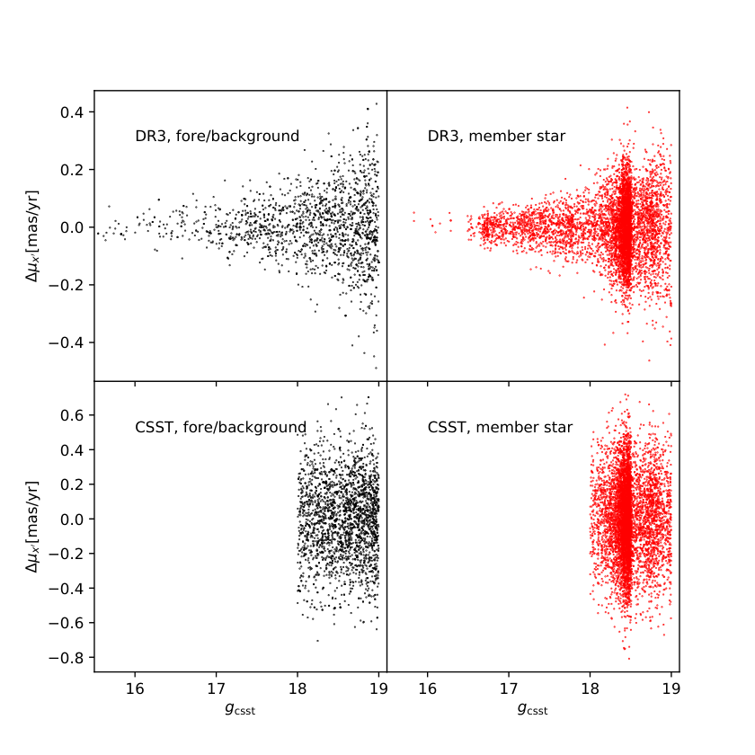
In our analysis, we first use true positions and velocities of 6,000 bound star particles without including realistic errors. In this way we can better understand the intrinsic systematic uncertainties behind the model. We will then repeat our analysis for only 2,000 bound star particles with only line-of-sight velocities plus typical errors. This is for more practical meanings, because the number of observed member stars in their host dwarfs is at most 2,000 for current observations, most of which do not have accurate proper motion measurements. Moreover, for the six nearby Sagittarius dSph-like systems, we will incorporate realistic observational errors to both line-of-sight velocities and proper motions, and model the contamination of fore/background or unbound stars, with member stars selected based on the differences in their kinematics relative to the dwarf centers. This is going to be compared with the error free and fore/background free model performance. Lastly, we find most Sagittarius dSph-like systems are undergoing contractions due to the effect of tidal force. We will check whether the amount of contraction is observable after including the Gaia DR3 proper motion errors. We now introduce how the observational errors are incorporated and how the fore/background is modeled.
II.2.1 Assigning apparent magnitudes of individual stars
Star particles in current state-of-the-art simulations represent simple stellar populations (SSP), and thus we cannot directly use their stellar properties, such as the magnitudes and colors, to represent single stars, though we can still use the position and velocity information of star particles in the simulations. To assign each star particle the appropriate magnitude information and hence observational errors, we use the trilegal code (Girardi et al. 2005; Vanhollebeke et al. 2009; Girardi et al. 2012; Girardi 2016, Chen et al. in preparation) to generate populations of different types of stars based on the input star formation history (SFH), the age-metallicity relation (AMR) and the total stellar mass. The SFH of the Sagittarius dSph is taken from Weisz et al. 2014, and we calculate the AMR based on the closed-box model, which agrees well with real data (Layden & Sarajedini 2000, e.g.). For the other dwarfs, the magnitude information is only required when we generate realistic errors for the line-of-sight velocities of mock stars (the case of using 2,000 star particles as tracers). For them we simply use the same SFH and AMR as the Sagittarius dSph. This is approximately a reasonable choice for dwarf galaxies, because dwarfs are relatively old, and the differences in their SFH and AMR do not lead to significant variations in the magnitude distribution of member stars.
The filter response curve is for the China Space Station Telescope (Zhan 2011; Cao et al. 2018; Gong et al. 2019, CSST;) filter. The absolute magnitudes generated by trilegal are converted to apparent magnitudes according to the distance modulus of each dwarf galaxy with respect to the mock observer in the simulation (see Subsection II.1 above). In our analysis, we will incorporate typical proper motion errors from either Gaia DR3 or from CSST44 4 There are many ground based proper motion measurements (Ruiz et al. 2001; Munn et al. 2004; Gould & Kollmeier 2004; Tian et al. 2017; Tian et al. 2020; Qiu et al. 2021, e.g.), but the typical errors are not small enough for detecting internal kinematics of dwarf galaxies.. When adopting the Gaia errors, we convert CSST magnitudes to Gaia magnitudes based on an empirical and color dependent relation linking the filter of the Hyper Suprime-Cam survey (Miyazaki et al. 2018; Komiyama et al. 2018; Furusawa et al. 2018) to Gaia (Wang et al. 2019), assuming CSST filter is not very different from HSC filter. This is a reasonable approximation, according to the CSST and HSC filter response curves (Gong et al. 2019; Kawanomoto et al. 2018).
The total number of stars generated by trilegal is very large, while the number of star particles used as tracers and bound to each dwarf galaxy in the simulation is more limited (in our case we use a subset of 6,000 or 2,000 as mentioned above). We take those trilegal stars whose apparent magnitudes are in a certain range of apparent magnitudes at the corresponding distance of each dwarf, randomly select 6,000 or 2,000 of them, and assign their magnitudes to our tracer star particles. The magnitude range is chosen as (Gaia DR3 proper motion errors) or (CSST proper motion errors) for the Sagittarius dSph-like systems. These nearby systems can all have more than 6,000 stars with . The magnitude range is when using CSST proper motion errors, because stars brighter than will be saturated in CSST observations. In particular, when we repeat our analysis with the smaller sample of 2,000 star particles as tracers (line-of-sight velocities only and with typical errors), we only use dwarf galaxies which can have more than 2,000 mock stars observed above the given apparent magnitude thresholds55 5 This is based on the trilegal prediction, with the total stellar mass of the dwarf system in the simulation as the normalization. Note when we test the error-free case, we simply use all dwarfs, without considering whether they can have enough number of bright stars.. For this case, we choose the magnitude range of for nearby Sagittarius dSph-like systems, and the range is chosen as for more distant systems.
II.2.2 parallax, line-of-sight velocity and proper motion errors
According to the apparent magnitudes, we assign each star particle errors in parallax, line-of-sight velocity and proper motion. The parallax errors are the median Gaia DR3 errors at the corresponding magnitude (Gaia Collaboration et al. 2021; Gaia Collaboration et al. 2016). The errors of the line-of-sight velocities are linear interpolations between 1 and 10 km/s, assuming stars with have 1 km/s of errors in the line-of-sight velocity, while stars with have the 10 km/s error. The line-of-sight velocity errors are typical for current or future spectroscopic surveys such as the Dark Energy Spectroscopic Instrument (Allende Prieto et al. 2020; Yano et al. 2016; Rehemtulla et al. 2022, DESI). The errors in proper motions are either the median Gaia DR3 errors or the typical CSST errors at the corresponding magnitudes.
For CSST, details about how its proper motion errors are modeled and predicted will be presented in a separate paper (Nie et al., in preparation). Nie et al. generated mock stars in the Galactic bulge region, and realistic star images are created at different epochs after including PSF, noise due to correction of flat and bias, readout noise, sky background, parallax and stellar motions. The process of source detection and centroid position determination at different epochs are then modeled. After calibrating the reference frame using mock reference stars, the final astrometric solutions and associated errors are obtained. The reference stars are assumed to have proper motions available from Gaia. Details about the distribution of reference stars, relevant CSST instrument parameters, how the mock star samples, stellar motions and PSF are modeled can be found in Nie et al. Moreover, their PSF model is simplified, which might be different from the real PSF during real operations. Based on about six times of astrometric measurements evenly distributed in 10 years of baseline, the typical proper motion error is 0.2 mas/yr at . Note because the number density of member stars in dwarf galaxies is less dense than the Galactic bulge region, their error is likely an upper limit. For Gaia, the median errors are obtained by querying the Gaia database, with typical DR3 proper motion error of 0.1 mas/yr at .
After realistic observational errors are obtained, the proper motion, distance and line-of-sight velocity of each star particle are displaced from their true values according to the assigned errors, by adding a displacement drawn from a Gaussian distribution with the standard deviation equaling to the corresponding error.
II.2.3 Modelling of fore/background and unbound star contamination
After observational errors are incorporated, we select as tracers those star particles whose differences in line-of-sight velocities, proper motions and parallaxes with respect to the dwarf centers66 6 Mass weighted mean coordinates and velocities of all bound particles belonging to the dwarfs, are all smaller than five times the corresponding errors (Vasiliev & Belokurov 2020, e.g.). In this way not only those true bound star particles are selected as tracers, but also some foreground and background particles as well as unbound particles around the dwarfs are included. To assign magnitudes for fore/background and unbound particles, we adopt the sample of stars created by trilegal for our Milky Way, and only use those stars in a rectangular region approximately centered on the observed Galactic latitude and longitude of the Sagittarius dSph ( and ). We randomly select a subsample of trilegal stars and assign their magnitudes to fore/background and unbound star particles in the simulation. The observational errors for fore/background and unbound particles are generated in the same way as for bound member star particles based on their apparent magnitudes.
Notably, for Sagittarius dSph-like systems, almost all bound star particles will be selected as tracers in this way, and we ensure these bound tracers to be the same as the subset used in the error-free case, for fair comparisons. Other selected unbound star particles are randomly picked up in proportional to the number of selected fraction of bound star particles.
Figure 1 shows the differences between the proper motions after assigning errors and the true proper motions (Au16-9), as a function of the apparent magnitudes and for both Gaia DR3 and CSST proper motion errors. The scatter is a factor of two smaller for Gaia DR3 errors than CSST errors at , and is smaller than 0.1 mas/yr at for Gaia DR3. The dense clump of stars in the right panels and at corresponds to the red giant branch bump, whereas there are no such prominent features in the sample of fore/background stars in the left panels.
III Methodology
Jeans Anisotropic Multi-Gaussian Expansion (jam) is a publicly available source of code77 7 http://github.com/lauralwatkins/. It is a powerful tool to constrain both the underlying matter distribution and the internal dynamics of tracers (Zhu et al. 2016b, e.g.), based on either line-of-sight velocities or proper motions of tracers. The version of jam we use for this paper is slightly different from the public version of the jam model for discrete data Watkins et al. 2013, with improved python interface and plotting tools. Details about jam can be found in Cappellari 2008 and Watkins et al. 2013, and here we only briefly introduce the method.
The method is based on solving the axis-symmetric Jeans equation in an intrinsic frame defined on the dwarf galaxy with cylindrical coordinates, to solve for the first and second velocity moments.
| (1) |
| (2) |
where is the tracer density distribution. is the total potential. Upon solving the equation to obtain unique solutions, the cross velocity terms are assumed to be zero, i.e., . In addition, the anisotropy parameter, , is assumed to be constant and defined as . A rotation parameter, , is introduced as .
In our analysis, we define the -axis of the intrinsic frame as the direction of the averaged spin of all bound star particles to the dwarf in the simulation, and the intrinsic frame is a right handed system. The intrinsic frame is linked to the observing frame (see Section II.1 above) through the inclination angle, , of the dwarf galaxy
| (3) |
and
| (4) |
where .
The total potential, , on the right hand side of Equations 1 and 2, is contributed by both luminous and dark matter. As we have mentioned, the luminous matter distribution is directly inferred from the surface brightness of the dwarf galaxy (see Section II.1 above). To model the density profile of dark matter, we adopt in our analysis either the NFW profile or a double power law functional form of
| (5) |
with the model parameters (, , and ) to be constrained. Note in our analysis throughout this paper, the outer power law index, , will be fixed to 3.
In order to have analytical solutions for any given potential model and tracer distribution, MGE is not only applied to the 2-dimensional surface density distribution of the luminous stellar component (see Section II.1.4 above), but also to the underlying model for the dark matter distribution and to the density distribution of tracers () as well88 8 In our case, tracers and the luminous stellar component have the same distribution, and therefore the same MGEs. Note the normalization of the MGE components for tracers is not important, which cancels out on two sides of the equations.. Each MGE component would have analytical solutions to Equations 1 and 2. In principle, each MGE component of the tracer population can have its own rotation parameter, , and velocity anisotropy parameter, . for each MGE component can also differ, but in our analysis we treat , and to be the same for different MGEs.
For an observed star with position on the image plane, which has observed velocity and error matrix of
| (6) |
its position, , can be transformed to the intrinsic frame to solve the corresponding velocities and velocity dispersions, based on a set of model parameters, . Solution for each MGE is sought, and solutions of different MGEs are added together in the end. The solutions are then transformed back to the observing frame. The mean velocity predicted by the model in the observing frame is denoted as , and the covariance matrix is defined through both the first and the second velocity moments
By assuming the velocity distribution predicted by the model is a tri-variate Gaussian with mean velocity and covariance at , the likelihood can be written as
| (10) |
In addition to the above model for the dwarf galaxy itself, the discrete jam model can also model a population of fore/background stars. The surface density of fore/background stars is assumed to be constant throughout the field of the dwarf, and is modeled to be a given fraction, , of the central surface density of the dwarf, . With the assumptions, the prior of dwarf membership can be written as
| (11) |
The velocity distribution of the fore/background stars can also be modeled as a tri-variate Gaussian with given mean velocity and velocity dispersions. Then the likelihoods of the dwarf and fore/background can be combined through
| (12) |
The total likelihood is the product of the likelihood for each star
| (13) |
The list of parameters used in our modeling are provided in the following:
(1) Rotation parameter, ;
(2) Velocity anisotropy, ;
(3) Stellar-mass-to-light ratio, ;
(4) Dark matter halo scale density, ;
(5) Dark matter halo scale radius, ;
(6) Inner density slope of the host dark matter halo, ;
(7) The background fraction, .
In particular, instead of directly fitting and , we fit and . This is to alleviate the degeneracy between the halo parameters and also make the parameter space to be more efficiently explored in log space (Zhu et al. 2016a). In our analysis, will mostly be fixed to unity, i.e, its true value, except for some cases which will be otherwise specified. The inner density slopes are also sometimes fixed to 1, i.e., for the NFW model profile. For fore/background contamination free cases, we fix to 0. Throughout this paper, we fix the distance and the inclination angle to be their true values. However, we have explicitly tested the results when the distance is allowed to be a free parameter. In this case, the best-constrained mass profiles remain very similar, while the best-fitting second velocity moments in very inner regions can be slightly improved, though the best-fitting distance might slightly differ from the true distance by up to 10%. Moreover, the outer density slope, , will be fixed to , but we have also tried to vary the outer slopes and add a constant background density, and our conclusions are not affected.
IV Results
IV.1 Overall performance
The left plot of Figure 2 shows the best-fitting versus true masses for all 28 dwarfs. We show this for the mass enclosed within the half-mass radius of tracers, , and the mass between 200 and 300 pc, . The fitting is based on the double power law model profile for the underlying dark matter (Equation 5) with free inner slopes. Note the matter density within 150 pc is often used as the proxy to the inner slopes (Read et al. 2019, e.g.). Unfortunately, 150 pc is below the resolution limit of auriga. So we focus on the radial ranges which are above the resolution limit for now, and we will investigate the constraint within 150 pc later in Section V.1, subject to extrapolations to the very center.
In general, is constrained better, with a scatter of 0.067 dex. This is in good agreement with the commonly accepted experience that the mass enclosed within the half-mass (or half-light) radius of tracers can be more robustly constrained upon dynamical modeling (Wolf et al. 2010; Walker & Peñarrubia 2011; Wang et al. 2015; Wang et al. 2020, e.g.). This is due to the degeneracy between the two halo parameters, and , reflecting that dynamical models mostly constrain the gravity or mass at the median radius of the tracers, but are less sensitive to the shape of the mass profile (Han et al. 2016a; Li et al. 2021; Li et al. 2022a, e.g.). There are a few cases for which are constrained slightly worse than , which are quite rare though.
is recovered reasonably, with a scatter of 0.167 dex, which is larger than the scatter of . We further classify systems into different groups according to their star formation activities. At first, we notice there are 11 star-forming systems with prominent galactic winds or gas outflows in the simulation, and on top of the corresponding red circles, we overplot green stars. An example of such outflows is shown in the left plot of Figure 15, which we will discuss later. There are another five systems with larger than zero star formation rates, but do not show obvious galactic winds, which we denote with blue diamonds. The six Sagittarius dSph-like (hereafter Sag-like) systems are demonstrated with cyan squares. Interestingly, systems classified in these groups show different trends. Quiescent Sag-like systems are more likely to have under-estimated, whereas the best-fitting for star-forming systems with strong outflows are biased to to be more above the black dashed line by 0.05 dex on average. The other systems are more symmetrically distributed on both sides of the black dashed line.
In the right plot of Figure 2, it is shown that the bias in best-fitting from the truth correlates with the specific star formation rate (sSFR). The correlation is weak or absent for . For the five systems with not zero star formation rates (SFR) but without prominent galactic winds, their sSFRs are weak, while the biases in their best fits are smaller on average. The six Sag-like systems are all quiescent with zero sSFR. Those systems with zero sSFR but are not too close to the galaxy center and are not yet undergoing strong tidal effects, i.e., not Sag-like, tend to show smaller biases in their best fits as well (red circles without star, diamond or square symbols).
In order to understand the cause for such a correlation between the bias in best fits and the sSFR, we provide in Figure 3 the best-fitting versus true masses between 200 and 300 pc in log space, versus the dynamical status of the systems (-axis) between 200 and 400 pc. In the -axis of Figure 3, is the radial action angle, or referred to as the phase angle by Han et al. 2016a; Han et al. 2016b. For a star at radius , is defined as
| (14) |
where is the radial period, is the radius at pericenter and is the radial velocity. Note when radial cuts are adopted in the tracer sample, the integral boundaries have to be properly changed accordingly. Equation 14 can be easily evaluated for a spherical potential. Here we at first calculate potential profiles for each dwarf based on the true radial distribution of all particles (star, dark matter, gas and black hole) under the spherical approximation, and we evaluate for each tracer star particle using the potential profile. Since our systems are not strongly deviating from spherical symmetry, the spherical assumption should approximately hold for most of our dwarfs, though not all. For a system in steady state, evaluated from the true potential is expected to distribute uniformly between 0 and 1, with the median value close to 0.5. The deviation of the medians from 0.5 thus indicates the amount of deviations from steady states. This is why the -axis quantity of Figure 3 is chosen as the median value of the for each system, which we denote as . The larger deviates from 0.5 (the black vertical dashed line), the stronger the system is deviating from the steady state.
We adopt particles between 200 and 400 pc to calculate the phase angles. The bias of best-fitting versus true correlates with the dynamical status over this range99 9 The choice of 200 to 400 pc is empirical. We choose a slightly larger outer radius of 400 pc than the outer radius for , i.e., 300 pc. This is because the orbits of tracers currently at larger radii can still extend to smaller radial range and affect the constraints there. However, we have checked other choices of radial ranges, such as 200 to 300 pc, 200 to 500 pc and 200 pc to 1 kpc, which all lead to some correlations between the bias in best fits and the corresponding dynamical status as well. Radial ranges larger than 1 kpc do not show any obvious correlation, which is partly because they do not fully represent the dynamical status in inner regions, and the recovery of the total mass between 200 to 300 pc mainly depends on tracers in more inner regions.. The scatter is large, but there exists the trend that systems more strongly deviating from steady states between 200 and 400 pc are on average more likely to have larger biases in . Explicitly, we find systems with under-estimated mostly tend to have larger than 0.5. In other words, their phase angle distribution is biased to large values. On the contrary, many systems with over-estimated tend to have smaller than 0.5, i.e., phase angle distribution is biased to small values, though some of them still have . Note for these systems with over-estimated and , we find part of them look a bit flattened, such as the blue diamond at the upper right corner (Au27-2), so the calculation of their might be slightly affected by the fact that we adopted spherical potential profiles to calculate their phase angles, but the overall trend is reasonable.
Nevertheless, Figure 3 unambiguously indicates that the amount of bias in best fits is related to the dynamical status of the systems, and thus the correlation between the bias in best fits and the sSFR reflects the dynamical status behind1010 10 The deviation of can be caused by either a) is evaluated with the correct potential, but tracers or the system are not in steady states; b) is evaluated for steady state tracers but with the wrong potential. In our case, it is the former.. For systems with strong galactic winds, despite the fact that wind particles are not used as tracers in our analysis, the galactic winds have caused deviations from steady states, resulting in larger biases (mostly over-estimates in in their best fits). For the other five systems with larger than zero but weak star formations, perhaps because they do not present prominent outflows to disturb the system, they tend to be closer to steady states on average and also have smaller biases in the best fits.
On the other hand and very interestingly, we find many of the Sag-like systems are undergoing some level of contractions along the longer image axis1111 11 For Au16-9, it is the -axis, while for the other systems, it is the -axis. The or major axis of the image plane, which is defined through the spin direction, usually corresponds to the longer axis for systems which are not strongly triaxial. However, due to the mis-alignment between the spin axis and the minor axis of the dwarf systems (see Section II.1), sometimes the image major/ axis is slightly shorter than the minor/ axis. When it happens, the difference between and axes is usually very small, such as Au16-9. If the difference is big, the systems are strongly triaxial and are thus excluded from our sample., which perhaps result in the under-estimated . These include Au16-9, Au23-7 and Au24-24, as marked in the figure with corresponding numbers. An example of the contraction is shown in the left panel of Figure 14 for Au16-9, which we will discuss later. In addition to the three systems, the other three Sag-like systems in Table 1 (Au21-10, Au23-4 and Au27-25) show less significant underestimates in . We only see some very weak contractions along the axis for Au21-10 and Au23-4, and this is perhaps why the best fits for the two dwarfs agree better with the truth. Au27-25 undergoes strong expansions along the and axes, and along the axis, it shows contractions. Note the expansion is not due to galactic winds as all the Sag-like systems have zero SFR and no wind particles.
The contractions and expansions in these Sag-like systems are due to the strong tidal effects at small distances. In fact, all six Sag-like systems are undergoing some expansions along the line of sight. This is expected, because the tidal disruption happens along the radial direction pointing to the galaxy center, and although the artificial observer is 8 kpc away from the galaxy center, the line-of-sight direction still aligns with the radial direction. As shown by Ogiya et al. 2022, when the dwarf is close to its peri-centric passage, the effective radius first undergoes a small decrease, followed by a large increase, sometimes associated with oscillations. On the contrary, if without tidal forces, Ogiya et al. 2022 showed that the effective radius stays almost constant.
Our results seem to indicate, strong tidal effects, which can cause both contractions and expansions, tend to cause underestimates in , and perhaps it is the contraction that is more related to the under-estimated . Perhaps the coherent contractions have caused smaller velocity dispersions in inner regions and hence under-estimated inner profiles. Besides, due to the global contraction, the apocenters of tracer orbits likely move inwards with time, resulting in greater than 0.5 if is evaluated based on the current underlying potential. This is because, the potential changes with time, but the apocenters will be over-estimated if they are calculated from the current potential by assuming that the potential does not evolve (steady state). On the other hand, outwards motions or expansions, such as the gas outflows or galactic winds, are more likely to cause overestimates in . The galactic winds cause lowered density in central regions, driving the whole system out of equilibrium. When is evaluated based on the current potential, assuming the system is in steady state, the distribution of is biased to be smaller, with less than 0.5.
In the next subsection, we move on to perform more detailed investigations on the best fits for the six quiescent Sag-like systems and another four star-forming systems with strong outflows.
IV.2 Examples of the best-fitting matter density profiles
In this subsection, we further investigate the best-fitting and true density profiles for six Sag-like systems and other four systems with prominent galactic winds.
IV.2.1 Best-fitting density profiles and velocity maps for Sagittarius dSph-like systems
We start with the six Sag-like systems. In Figures 2 and 3, we have shown that the best-fitting masses between 200 and 300 pc, , are under-estimated for the six systems and to different levels, when using the double power law model profile for the underlying dark matter. In Figure 4, the best fits (magenta curves) based on the double power law potential model and true total mass profiles (green dots with errorbars) are shown for the six systems. For Au16-9, Au21-10, Au23-7 and Au24-24, their best-fitting inner profiles are lower than the truth, i.e., the magenta solid curves are below the green dots within 0.5 kpc, and the differences are significant compared with the small errorbars. of Au23-4 and Au27-25 are mildly under-estimated, so the differences between the magenta curves and the green dots are not very obvious in the corresponding panels.
is fixed to unity for the magenta curves, but the underestimates in the inner profiles remain the same, even if we allow to be free. Besides, we have fixed the outer slopes to be . However, the poor constraints in the outskirts are not improved if we allow the outer slopes to be free. This is probably due to the significantly smaller number of tracer star particles in outskirts. These systems mostly have over-estimated outer profiles and under-estimated inner profiles. The true and best-fitting profiles cross with each other at the radii close to the half-mass radii. Note although only bound particles are used as tracers, the true profiles in Figure 4 are calculated based on all particles at the corresponding radial ranges1212 12 Inclusion of unbound particles mainly affects the true profiles in outskirts, with the inner profiles barely affected. . This is because though particles belonging to the host halo might be approximated to have a constant density over the scale of the dwarf, they still contribute to the potential gradient. Since background particles belonging to the host halo could be more dominant for such nearby Sag-like systems, we have also tried to model the underlying matter distribution using the double power law model plus a constant density model. However, the best constrained model still tends to under-estimate the inner profiles and over-estimate the outer profiles.
We also show in Figure 4 the best-fitting star and dark matter profiles separately. The red, black and green curves are the best-fitting star, dark matter and total profiles based on the NFW model profile. Here is allowed to be free. It is clearly shown that the profiles of the stellar component, and hence , are poorly constrained by jam, with the best fits (red curves) significantly deviating from the truths (red diamonds) in most cases. The dark matter profiles, on the other hand, can be constrained better, but still show some significant deviations from the truth in inner regions, especially for Au23-4 and Au23-7. Fortunately, despite the relatively worse fits to the stellar and dark matter components individually, the total profiles can be fit significantly better.
Due to the poorly constrained , we have fixed to unity in Figures 2 and 3, when the double power law potential model is used. However, with the double power law model, we do have tried to allow to be free as well, though we choose not to explicitly show the results to avoid redundancy. Our conclusions remain very similar. The stellar and dark matter profiles are poorly constrained individually. Actually, with the free inner slopes in the double power law model, the fitting to the dark matter component can become significantly lower than the truth in inner regions for a few cases, whereas the stellar component is significantly over-estimated, with the total profiles (stellar dark matter) still more reasonably constrained. Hereafter, unless otherwise specified, will be fixed to unity, i.e., its true value. This is a reasonable operation, because observationally, can be alternatively constrained through stellar population synthesis modeling and fixed upon dynamical modeling.
The poor fits to stellar and dark matter profiles individually are mainly due to the degeneracy between and halo parameters. First of all, the true stellar and dark matter profiles share similar shapes in Figure 4. Note all particles have been included in these true profiles, and if only using bound particles, the stellar and dark matter profiles would appear more similar in outskirts. This is due to the strong tidal stripping happened to these Sag-like systems, making them have similar outer dark matter and stellar halo profiles (Errani et al. 2022, e.g.). As a result, the model has difficulties distinguishing the stellar and dark matter components, as they have similar contributions to the shape of the underlying potential profiles. This explains why the best fits to stellar and dark matter components are poor individually. Moreover, we show in Figure 5 the likelihood contours of different parameter combinations for Au16-9. The anti-correlations or degeneracies among and the two halo parameters ( and ) are prominent.
Comparing the magenta and green curves in Figure 4, we find the inner profiles are constrained worse when the double power law model profile is used, for Au16-9, Au21-10, Au23-7 and Au24-24, than the NFW profile. To explore why the inner profiles are constrained worse when the inner slopes are allowed to free, we check the best-fitting and true velocity maps in Figure 6, which shows the mean velocity and velocity dispersion profiles for the component and for Au16-9 as an example. Both the velocity and velocity dispersion profiles have large scatters, and the double power law model tends to go through the middle of the velocity dispersion profiles in inner regions, while the NFW model leads to a curve which is higher in the center. Both are reasonable fits, but in fact the double power law model achieves a better fit with log likelihood larger than that of the NFW model by 33, which is significantly larger than the expected 1- uncertainty of five free parameters. This is in fact benefited from our usage of a large sample of 6,000 member stars. While the velocity profiles are better fit with the double power law model profile, the deviation of the best-fitting double power law model from the true density profile is larger, which reflects the deviation from the steady state due to strong tidal effects, and thus a better fit to the velocity maps lead to a worse fit to the density profile. Explicitly, as we have mentioned, the strong contraction of member stars in Au16-9 (see Figure 14) has likely caused smaller velocity dispersions in inner regions, and thus the double power law model with under-estimated inner profiles fits better the velocity map. By using the NFW model, more masses are forced to be in the inner region, leading to a better match to the true density profile but a worse fit to the velocity map.
IV.2.2 Best-fitting density profiles and velocity maps for star-forming systems with outflows
Now we move on to discuss a few examples of star-forming systems with prominent outflows. Figure 7 shows the true and best-fitting total profiles for four representative star-forming systems. They all have strong outflows and large biases in their best-fitting . The four systems are marked with corresponding numbers in Figure 3. For simplicity, we do not show the profiles for the stellar and dark matter components, but only show the total profiles. These systems all have over-estimated inner density profiles and under-estimated outer profiles, with the true and best-fitting profiles cross at roughly the half-mass radii.
The mean velocity and velocity dispersion profiles of star particles for Au21-9 is shown in Figure 8, and we only show the component as an example. The apparent sizes of such distant star-forming dwarfs are smaller than nearby Sag-like objects in Figure 6. Overall, the agreement between the truth and the best fit is reasonable. The model tends to fit a rotation, i.e., positive along the positive -axis (minor axis) and negative along the negative -axis. These systems have strong galactic winds (wind particles), but the star particles do not show obvious signatures of outwards motions. However, there are some indications of inflows of the stars on large scales along the major axis, that is, is negative along the positive -axis (major axis) and positive along the negative -axis. Such inflows are perhaps due to tidal effects, because this dwarf is on its way of approaching host galaxy center. Besides, the stellar system can expand in response to the lowered potential due to gas outflows at the beginning, which undergoes some overshooting and as a result would contract and get stabilized later (Navarro et al. 1996; Li et al. 2022b, e.g.). Maybe we happen to observe this dwarf at the contraction stage. The best-fitting velocity dispersion along the major axis is slightly lower than the truth beyond 40′, while the best-fitting dispersion along the minor axis seems to be a bit higher in amplitude than the truth beyond 10′, which are perhaps related to the deviation from steady states in outskirts.
Comparing Figures 4 and 7, it seems both figures have the best-fitting and true total profiles crossing at approximately the half-mass radii. As we have mentioned, due to the degeneracy between the halo parameters, most dynamical models mainly constrain the mass at the median radius of the tracers, but are less sensitive to the shape of the mass profile. To maintain the relatively robust constraints on the mass at the half-mass radius of tracers, the biases in the best-fitting inner and outer density profiles for the same system often happen in opposite ways. In addition, quiescent Sag-like systems and star-forming systems also tend to have opposite trends. Sag-like systems tend to have under-estimated inner profiles and over-estimated outer profiles, whereas star-forming systems with prominent outflows tend to have over-estimated inner profiles and under-estimated outer profiles. This is because, as we have explained in the previous subsection, the contractions/expansions (perhaps mainly the contractions) due to strong tidal effects for nearby Sag-like systems and galactic winds/gas outflows for more distant star-forming systems drive the systems out of equilibrium, but in opposite ways.
IV.3 Constraints based on less tracers and only line-of-sight velocities with observational errors
Our results in the previous sections are based on a large sample of 6,000 star particles as tracers, with both line-of-sight velocities and proper motions, but without errors. The error-free and large sample of tracers have enabled us to control the size of statistical errors while focus on investigating the intrinsic systematics behind jam. However, current observations of nearby dwarf galaxies at most provide kinematical information of 2,000 member stars (Zhu et al. 2016a, e.g.), most of which do not have accurate proper motion measurements. Thus for more practical meanings, in this subsection we repeat our analysis by using a smaller sample of 2,000 star particles as tracers, and we only use their line-of-sight velocities after including observational errors (see Section II.1 for details). After excluding distant systems which cannot have more than 2,000 stars brighter than , we end up with 16 systems.
The best constrained versus their true values is shown in Figure 9. We overplot the error-free constraints based on 6,000 star particles as black empty triangles. Approximately, it seems can still be constrained ensemble unbiasedly, but compared with the measurements based on 6,000 star particles and both line-of-sight velocities and proper motions, the measurements now slightly biased more above the diagonal reference line at . The scatter is increased by 50%, with the black triangles having a scatter of 0.169 dex1313 13 This is slightly different from the scatter of red circles in the left plot of Figure 2, due to the exclusion of distant systems with less than 2,000 bright stars. and the red circles having a scatter of 0.260 dex. Our results thus indicate that systematic uncertainties caused by deviations from the steady states of the dwarf systems are dominating the final errors of mass estimation. If without accurate proper motion measurements, line-of-sight velocities of 2,000 tracers with typical observational errors can still achieve reasonable and approximately ensemble unbiased measurements for on average, but with slightly larger scatters.
IV.4 Constraints on Sagittarius dSph-like systems after including observational errors and unbound star contamination
In the previous subsections, our results are based on bound star particles as tracers. In this section we discuss the results after incorporating line-of-sight velocity errors, Gaia DR3 parallax errors and either Gaia DR3 or CSST (Zhan 2011; Cao et al. 2018; Gong et al. 2019, CSST;) proper motions errors. We also select member stars according to their kinematics. We first present results based on Gaia DR3 errors for the six Sag-like systems. We then move on to show results based on the CSST proper motion errors for the dwarf with the closest distance to the mock observer (Au16-9).
After including typical line-of-sight velocity errors, Gaia DR3 proper motions and parallax errors, we select tracer star particles based on their differences in proper motions, line-of-sight velocities and parallaxes with respect to the dwarf centers (see Section II.2 for details), and the best fits are shown as blue dashed curves in Figure 10 for the six Sag-like systems. Stars selected in this way not only include those true bound member stars, but may also include fore/background contamination and some unbound star particles at the vicinity of the dwarf. As we have explicitly checked, because the associated observational errors are relatively small for such nearby Sag-like systems, the fraction of actual foreground or background stars is very small. In addition to bound member stars, most of the other tracer stars selected in this way are those unbound star particles surrounding the dwarf system. Part of these star particles might once be bound to the dwarf, and have been stripped by the host halo recently.
After including observational errors and contamination by unbound stars, the uncertainties as indicated by the blue shaded regions are now significantly larger than the original magenta shaded regions, but the best fits stay very similar to the original error-free best fits. On the basis of the blue dashed curves, yellow and cyan dashed curves are best fits using only proper motion data or using only line-of-sight velocities, respectively. For Au16-9, Au21-10, Au23-4 Au24-24 and Au27-25, results based on pure proper motions and pure line-of-sight velocities are consistent with each other within 1-. However, for Au23-7, pure proper motions and pure line-of-sight velocities show more significant differences. Interestingly, the yellow curves, i.e., with pure proper motions, show much better agreement with the true profiles. The larger difference between the yellow and cyan curves for Au23-7 is mainly related to how the tracer stars are selected. We found those unbound star particles selected as tracers and mainly in outskirts for this systems show larger velocity dispersions in their line-of-sight velocities than those of bound particles. The line-of-sight velocity distribution of these particles also deviates from the assumed Gaussian distribution by jam, and jam does not model them as background. As a result, the increased velocity dispersions lead to the much higher amplitudes in outskirts of the best fits, when both line-of-sight velocities and proper motions are used and when only line-of-sight velocities are used, but is not the case when only proper motions are used.
Our results indicate that, for such nearby Sag-like systems, we can observe enough number of bright stars, and with the accuracy of Gaia DR3 errors, proper motions can be as useful as or even sometimes better than line-of-sight velocities. For example, for Au16-9 at slightly beyond 20 kpc, the typical Gaia DR3 proper motion error of 0.1 mas/yr corresponds to error in tangential velocity of 5 km/s, which is comparable to the typical error of 1 to 10 km/s for the line-of-sight velocity. We have repeated our analysis by incorporating observational errors for more distant dwarf galaxies. Unfortunately, for systems close to or beyond 100 kpc, the number of bright stars is limited, and Gaia DR3 proper motion errors are not good enough to achieve reasonable constraints, with the fitting based on pure proper motion data very difficult to converge. This is expected, because most stars with have typical Gaia DR3 errors of 0.1 mas/yr, which corresponds to 40 km/s of errors in tangential velocities at 80 kpc, and thus are useless.
However, the precision in future Gaia proper motion data is expected to be improved in a way proportional to ( is the time), indicating more than a factor of two reduction in error for DR4 compared with DR3, and additionally a factor of 2.8 of improvement for the extended mission compared with the end of the 5-year mission at fixed magnitude, pushing to a limit which can even be better than the typical line-of-sight velocity errors (Mateu et al. 2017; Brown 2021, e.g.). This means, based on pure proper motion data, dynamical modelings, which can only be achieved for nearby Sag-like systems at 50 to 60 kpc for the furthest now, is very promising to be applied to enough number of fainter tracers in dwarf systems at or beyond 100 kpc in the future.
We now investigate the expected performance of using future CSST proper motions. The expected upper limit in CSST proper motion error (0.2 mas/yr) is about a factor of two larger than that of Gaia DR3 at . For very nearby systems such as Au16-9 at a distance a bit more than 20 kpc, the corresponding tangential velocity error is 10 km/s , which quickly increases to 40 km/s beyond 40 kpc. Thus it seems dynamical modeling with pure proper motion data is difficult with 0.2 mas/yr of error for systems more distant than 3040 kpc. In Figure 11, we show the constraint based on the typical CSST proper motion error for Au16-9 as an example. The uncertainties are significantly larger, but the usage of pure proper motion data still leads to a reasonable fit.
The typical CSST proper motion error is based on about six astrometric measurements evenly distributed in 10 years of baseline. Our results thus indicate that this particular observational strategy would provide useful proper motions for dynamical modeling of very nearby systems at distances 20 kpc. However, due to the fact that the CSST proper motion error estimates are based on the star number density in the Galactic bulge region, the actual errors based on the same operational mode can be smaller, so with pure CSST proper motion data, it could be possible to push slightly further. Notably, as will be shown in Nie et al., the associated proper motion errors increase slowly towards fainter magnitudes, reaching 0.4 mas/yr at CSST -band apparent magnitude of 24-th, whereas Gaia proper motion errors increase very quickly beyond . This is because the aperture and exposure time of CSST is designed to have higher signal-to-noise ratios at fainter magnitudes than Gaia, with the -band limiting magnitude of about 26 to 27 (Zhan 2011). Thus future CSST proper motion measurements are promising to compensate Gaia measurements at fainter magnitudes.
V Discussions
V.1 Connection to the core-cusp problem
The softening scale of the level 3 auriga set of simulations is 185 pc at . For radial range below this scale, the density profiles and dynamics of tracer particles are not realistic, so it is difficult for us to directly reach the scale that is the most relevant to the core-cusp problem (Read et al. 2019, 150 pc; e.g.). However, based on our results in the previous section, the best-fitting inner density profiles show different amount of biases for individual systems, which also show a dependence on the star formation activities. It seems similar biases would exist on scales below the resolution limit as well, and thus we should be cautious when interpreting the results for individual systems.
In Section IV.2, the best-fitting inner profiles of a few quiescent Sag-like systems are shown to be below the true profiles when the inner slopes are allowed to be free. An interesting case is Au16-9. For this system, both the NFW and the double power law model profile lead to reasonable fits to the velocity map, but the qualitative goodness of fit is significantly better for the double power law model. Despite of the better fit to the tracer kinematics, the actual inner density profile is significantly under-estimated. Such an inconsistency between the kinematical prediction and the actual density distribution indicates strong deviations from steady states. Violation of the steady-state assumption could result in more core-ish inner profiles when the truth is more cuspy for individual systems. Au16-9 is close to the galactic center and is undergoing some prominent contractions due to strong tidal effects, and we should avoid using systems which are strongly out of equilibrium, otherwise we may end up drawing wrong conclusions regarding the core-cusp issue, especially when looking at individual or small sample of systems.
In real observation, instead of directly constraining the inner slopes, the best-fitting total mass within 150 pc, , is often adopted to infer the steepness of the inner slope (Read et al. 2019, e.g.). We now compare the best-fitting and true mass within 150 pc. To achieve the comparison, we extrapolate the actual density profiles in the simulation down to scales below the resolution limit, based on the double power law model profile. The extrapolation is used to calculate , which is regarded as the truth. On the other hand, the best-fitting mass within 150 pc, , is measured through tracer dynamics beyond 185 pc, extrapolated to the central region. Here we have excluded tracers within 185 pc to avoid wrong dynamics. Note in previous sections, our discussions are focused on the radial range not affected by star particles within 185 pc, and thus including or excluding tracers within 185 pc barely affects our results.
The results are shown as red circles in Figure 12. The associated uncertainties in the true masses are computed according to the boundaries which enclose 68% of the MCMC chains1414 14 When fitting the double power law function to the true density profiles to achieve the extrapolation, we use emcee. . Because there are no reliable tracers within 185 pc, now the jam constrained through stellar dynamics has significantly larger errorbars than those of and in previous plots. For convenience, we also overplot the black empty triangles which are the measurements for .
The scatter in is 0.255 dex, which is larger than the scatter of (0.167 dex), but the overall fitting is reasonable. Star-forming and quiescent systems are well separated, with quiescent systems having smaller . We believe the amount of scatter for red circles in Figure 12 is an upper limit, because the scatter can be further decreased if tracers within 150 pc are available, and indeed in real observations stars within 150 pc can be observed and used for dynamical constraints.
We now check whether can be used as a good proxy to the inner slopes. Here we calculate the true inner slopes, , based on the best-fitting parameter of the double power law model profile to the actual total density profiles beyond 185 pc in the simulation, so depends on extrapolations to the very center. Figure 13 shows versus both and . The scatters and errorbars are large, but there are correlations between and or . In the left plot, increases for steeper , indicating has the potential of being used as the proxy to infer the inner slopes. In the right plot, the correlation between and seems to be weakened due to the scatter in the recovery of . However, we emphasize that since we do not have tracers within 150 pc, the scatter in the right plot of Figure 13 and in Figure 12 is likely an upper limit. If tracers within 150 pc are available, the scatter is likely to be decreased.
V.2 The detectability of contractions and outflows
In Section IV, we discussed the contractions of member stars due to strong tidal effects for nearby systems, and star-forming systems are also mentioned to have outflows. Such systems are strongly out of equilibrium, and thus caution has to be taken if using them for dynamical modeling. Hence observational identifications of such contractions and outflows are important. In this subsection, we briefly discuss the detectability of such motions.
To detect isotropic contractions or expansions, the usage of line-of-sight velocities of member stars or IFU observation might not be very useful, because the effect would be averaged and canceled out along the line-of-sight direction. In addition, if the contraction mainly happens along the image longer axis but not along the line-of-sight direction as in our case, line-of-sight velocities will not be helpful either. Proper motions thus become more important.
In the left plot of Figure 14, we show the contraction of member stars of Au16-9, without including any observational errors. It is clearly shown that is negative/positive along the positive/negative -axis (minor axis), which demonstrates the contraction1515 15 Since along the major and minor axes, only stars within sectors of degrees to the corresponding axes are used to make the plot, binned along the direction is dominated by radial motions. It is very prominent that is negative along the positive minor axis, and positive along the negative minor axis (or -axis), which reflect inwards motions or contractions.. Note the minor axis of Au16-9 is in fact the longer image axis, because our image major axis is defined according to the spin direction (see Section III for details), but the difference between the image major and minor axes of Au16-9 is very small anyway. Besides, along the image major axis tends to show some rotations, but the rotation is absent in Figure 6, indicating Au16-9 could be triaxial.
In the middle plot of Figure 14, we include Gaia DR3 proper motion errors (see Section II.2 for details), the signal is noisier but still clearly detectable. In the right plot, not only the proper motion errors are included, but also the stellar tracers are selected according to their difference in kinematics with respect to the dwarf center. The inclusion of some unbound particles in outskirts has caused some offsets towards negative . This is because the global motion of the dwarf is defined through bound star particles and subtracted off from all selected tracer particles. However, those unbound particles are not expected to have zero mean velocity after the subtraction. Despite of the offset, the contraction is still detectable.
Our results indicate, promisingly, that current Gaia DR3 proper motion errors can enable us to detect such contraction motions for member stars of nearby Sag-like systems. The detection is also benefited from the usage of a large sample of 6,000 member stars.
In contrast to the detection of global contractions in nearby systems, the detection of gas outflows can be more challenging. The 11 dwarfs with gas outflows are at fairly large distances. The most nearby dwarf with such outflow is at 130 kpc. Figure 15 shows the major and minor axis proper motions of wind particles around this dwarf. In the left plot, no observational errors are incorporated, and we can clearly see the expansions, i.e., the tangential velocities are positive at the positive -axis and negative at the negative -axis (black dots with errorbars). We now simply incorporate the Gaia DR3 proper motion errors to these wind particles in the right plot, treating them as individual stars. The trend becomes significantly noisy, but the signal is still marginally detectable for this system at 130 kpc. In real observation, the detection of such gas outflows perhaps has to depend on observations of the hot gas distribution around these dwarfs at different epochs.
VI Conclusions
In this study, we construct mock samples of member stars for 28 simulated dwarf galaxies from the cosmological level 3 set of auriga simulations. We applied the discrete axis-symmetric Jeans Anisotropic Multi-Gaussian Expansion (jam) modeling method to the 28 dwarf systems, to recover the underlying mass distribution through the stellar dynamics under the steady-state assumption. Among our sample of dwarf galaxies, there are 6 nearby Sagittarius dSph-like (Sag-like) systems and other 11 star-forming systems with strong galactic winds or gas outflows.
We first use 6,000 bound member star particles without errors as stellar tracers for each system, which is to ensure good statistics. After assigning star particles apparent magnitudes using the multi-population synthesis trilegal code, we incorporate typical line-of-sight velocity errors (110 km/s), Gaia DR3 parallax errors and Gaia DR3 or China Space Station Telescope (CSST) proper motion errors. We also try a smaller sample of 2,000 star particles as tracers and try to select stellar tracers according to their differences in kinematics to the dwarf centers.
Compared with the true matter distribution in the simulation, we find the recovered density profiles of the stellar and dark matter components individually are poor due to the degeneracy between stellar mass and dark matter distribution, and the constraints on the stellar-mass-to-light ratios are very weak. Fortunately, the density profiles of the total mass distribution can be constrained more reasonably.
The total mass within the half-mass radius of tracers can be constrained the best, with a scatter of 0.067 dex. The best-fitting masses between 200 and 300 pc, , are recovered ensemble unbiasedly, with a scatter of 0.167 dex. However, the amount of bias shows a dependence on the current specific star formation rate (sSFR). This is a result of the deviation from steady states. Most quiescent Sag-like systems undergoing strong tidal effects have their under-estimated than the truth, whereas most star-forming systems with outflows have over-estimated.
The dependence of the best fits on sSFR reflects how tidal effects and galactic winds (gas outflows) perturb the system, driving it away from the steady state. We discover that most of the member stars in Sag-like systems have contractions along the image longer axis, which are the outcomes of strong tidal effects (Ogiya et al. 2022, e.g.) and cannot be properly modeled by equilibrium models. On the other hand, the strong galactic winds or gas outflows in star-forming systems have driven the system out of equilibrium as well, despite the fact that wind particles themselves are not directly used as tracers. Tidal effects and galactic winds both cause the deviation from steady states, but in opposite ways, resulting in under-estimated and over-estimated inner density profiles, respectively. When talking about individual systems, one might end up with cored constraints on the inner profiles, whereas the truth is, on the contrary, more cuspy. On the other hand, cored systems might also be constrained as cuspy in the best fits for individual systems. Thus one should avoid drawing strong conclusions based on individual or limited number of systems. Instead, the averaged result based on a relatively large sample of dwarf galaxies is ensemble unbiased and more robust.
Interestingly, systems which still have some amount of star formation, but without prominent outflows, mostly show smaller amount of biases in their best fits. Besides, massive quiescent systems at large distances and are not yet undergoing strong tidal effects, i.e., not Sag-like, also show smaller amount of biases on average. When using dynamical models based on the steady state assumption, we should be cautious when using systems undergoing prominent contractions or expansions, which are strongly out of equilibrium. Promisingly, with Gaia DR3 proper motion errors, the contraction in nearby Sag-like systems is shown to be detectable.
Using a smaller sample of 2,000 star particles with only line-of-sight velocities (typical errors from 1 to 10 km/s) as tracers, can still be constrained ensemble unbiasedly, but the scatter is increased by 50%.
After incorporating realistic observational errors (proper motion errors correspond to Gaia DR3) and selecting tracer stars based on the differences in their kinematics with respect to the dwarf center, we find their best constrained density profiles agree with the error-free constraints within 1-. For such nearby dwarf systems, dynamical constraints based on pure proper motions with Gaia DR3 errors perform equally well or even better than the case of using pure line-of-sight velocities, which is very encouraging. On the other hand, the expected upper limit in proper motion errors for the future CSST survey is about twice larger than that of Gaia DR3, at CSST -band apparent magnitudes of , which can already lead to reasonable constraints for very nearby systems at distances 20 kpc.
By extrapolating the true density profiles in the simulation down to the radial range below the resolution limit, and by extrapolating the best-fitting density profiles based on tracer dynamics at pc down to the center, we find the mass within 150 pc can be recovered ensemble unbiasedly as well, but with a larger scatter of 0.255 dex. We also see correlations between the best-fitting or true mass within 150 pc and the true inner slopes, but with large scatters. The scatter can be improved if tracers within 150 pc are available.
References
- Allende Prieto et al. (2020) Allende Prieto, C., Cooper, A. P., Dey, A., et al. 2020, Research Notes of the American Astronomical Society, 4, 188, doi: 10.3847/2515-5172/abc1dc
- Boldrini (2022) Boldrini, P. 2022, arXiv e-prints, arXiv:2201.01056. https://arxiv.org/abs/2201.01056
- Boylan-Kolchin et al. (2011) Boylan-Kolchin, M., Bullock, J. S., & Kaplinghat, M. 2011, MNRAS, 415, L40, doi: 10.1111/j.1745-3933.2011.01074.x
- Brown (2021) Brown, A. G. A. 2021, ARA&A, 59, doi: 10.1146/annurev-astro-112320-035628
- Bullock & Boylan-Kolchin (2017) Bullock, J. S., & Boylan-Kolchin, M. 2017, ARA&A, 55, 343, doi: 10.1146/annurev-astro-091916-055313
- Campbell et al. (2017) Campbell, D. J. R., Frenk, C. S., Jenkins, A., et al. 2017, MNRAS, 469, 2335, doi: 10.1093/mnras/stx975
- Cao et al. (2018) Cao, Y., Gong, Y., Meng, X.-M., et al. 2018, MNRAS, 480, 2178, doi: 10.1093/mnras/sty1980
- Cappellari (2008) Cappellari, M. 2008, MNRAS, 390, 71, doi: 10.1111/j.1365-2966.2008.13754.x
- Cappellari et al. (2013) Cappellari, M., Scott, N., Alatalo, K., et al. 2013, MNRAS, 432, 1709, doi: 10.1093/mnras/stt562
- Cole et al. (2005) Cole, S., Percival, W. J., Peacock, J. A., et al. 2005, MNRAS, 362, 505, doi: 10.1111/j.1365-2966.2005.09318.x
- de Blok (2010) de Blok, W. J. G. 2010, Advances in Astronomy, 2010, 789293, doi: 10.1155/2010/789293
- de Blok et al. (2001) de Blok, W. J. G., McGaugh, S. S., & Rubin, V. C. 2001, AJ, 122, 2396, doi: 10.1086/323450
- Errani et al. (2022) Errani, R., Navarro, J. F., Ibata, R., & Peñarrubia, J. 2022, MNRAS, 511, 6001, doi: 10.1093/mnras/stac476
- Faucher-Giguère et al. (2009) Faucher-Giguère, C.-A., Lidz, A., Zaldarriaga, M., & Hernquist, L. 2009, ApJ, 703, 1416, doi: 10.1088/0004-637X/703/2/1416
- Feast et al. (1961) Feast, M. W., Thackeray, A. D., & Wesselink, A. J. 1961, MNRAS, 122, 433, doi: 10.1093/mnras/122.5.433
- Flores & Primack (1994) Flores, R. A., & Primack, J. R. 1994, ApJ, 427, L1, doi: 10.1086/187350
- Foot & Vagnozzi (2015) Foot, R., & Vagnozzi, S. 2015, Phys. Rev. D, 91, 023512, doi: 10.1103/PhysRevD.91.023512
- Freundlich et al. (2020a) Freundlich, J., Dekel, A., Jiang, F., et al. 2020a, MNRAS, 491, 4523, doi: 10.1093/mnras/stz3306
- Freundlich et al. (2020b) Freundlich, J., Jiang, F., Dekel, A., et al. 2020b, MNRAS, 499, 2912, doi: 10.1093/mnras/staa2790
- Furusawa et al. (2018) Furusawa, H., Koike, M., Takata, T., et al. 2018, PASJ, 70, S3, doi: 10.1093/pasj/psx079
- Gaia Collaboration et al. (2016) Gaia Collaboration, Prusti, T., de Bruijne, J. H. J., et al. 2016, A&A, 595, A1, doi: 10.1051/0004-6361/201629272
- Gaia Collaboration et al. (2021) Gaia Collaboration, Brown, A. G. A., Vallenari, A., et al. 2021, A&A, 649, A1, doi: 10.1051/0004-6361/202039657
- Genina et al. (2022) Genina, A., Read, J. I., Fattahi, A., & Frenk, C. S. 2022, MNRAS, 510, 2186, doi: 10.1093/mnras/stab3526
- Genina et al. (2018) Genina, A., Benítez-Llambay, A., Frenk, C. S., et al. 2018, MNRAS, 474, 1398, doi: 10.1093/mnras/stx2855
- Genina et al. (2020) Genina, A., Read, J. I., Frenk, C. S., et al. 2020, MNRAS, 498, 144, doi: 10.1093/mnras/staa2352
- Gentile et al. (2004) Gentile, G., Salucci, P., Klein, U., Vergani, D., & Kalberla, P. 2004, MNRAS, 351, 903, doi: 10.1111/j.1365-2966.2004.07836.x
- Girardi (2016) Girardi, L. 2016, Astronomische Nachrichten, 337, 871, doi: 10.1002/asna.201612388
- Girardi et al. (2005) Girardi, L., Groenewegen, M. A. T., Hatziminaoglou, E., & da Costa, L. 2005, A&A, 436, 895, doi: 10.1051/0004-6361:20042352
- Girardi et al. (2012) Girardi, L., Barbieri, M., Groenewegen, M. A. T., et al. 2012, in Astrophysics and Space Science Proceedings, Vol. 26, Red Giants as Probes of the Structure and Evolution of the Milky Way, 165, doi: 10.1007/978-3-642-18418-5_17
- Gong et al. (2019) Gong, Y., Liu, X., Cao, Y., et al. 2019, ApJ, 883, 203, doi: 10.3847/1538-4357/ab391e
- Gould & Kollmeier (2004) Gould, A., & Kollmeier, J. A. 2004, ApJS, 152, 103, doi: 10.1086/382529
- Grand et al. (2017) Grand, R. J. J., Gómez, F. A., Marinacci, F., et al. 2017, MNRAS, 467, 179, doi: 10.1093/mnras/stx071
- Grand et al. (2018) Grand, R. J. J., Helly, J., Fattahi, A., et al. 2018, MNRAS, 481, 1726, doi: 10.1093/mnras/sty2403
- Han et al. (2016a) Han, J., Wang, W., Cole, S., & Frenk, C. S. 2016a, MNRAS, 456, 1003, doi: 10.1093/mnras/stv2707
- Han et al. (2016b) —. 2016b, MNRAS, 456, 1017, doi: 10.1093/mnras/stv2522
- Han et al. (2015) Han, J., Eke, V. R., Frenk, C. S., et al. 2015, MNRAS, 446, 1356, doi: 10.1093/mnras/stu2178
- Hayashi et al. (2020) Hayashi, K., Chiba, M., & Ishiyama, T. 2020, ApJ, 904, 45, doi: 10.3847/1538-4357/abbe0a
- Henriques et al. (2012) Henriques, B. M. B., White, S. D. M., Lemson, G., et al. 2012, MNRAS, 421, 2904, doi: 10.1111/j.1365-2966.2012.20521.x
- Kaplinghat et al. (2020) Kaplinghat, M., Ren, T., & Yu, H.-B. 2020, J. Cosmology Astropart. Phys, 2020, 027, doi: 10.1088/1475-7516/2020/06/027
- Kawanomoto et al. (2018) Kawanomoto, S., Uraguchi, F., Komiyama, Y., et al. 2018, PASJ, 70, 66, doi: 10.1093/pasj/psy056
- Klypin et al. (1999) Klypin, A., Kravtsov, A. V., Valenzuela, O., & Prada, F. 1999, ApJ, 522, 82, doi: 10.1086/307643
- Komiyama et al. (2018) Komiyama, Y., Obuchi, Y., Nakaya, H., et al. 2018, PASJ, 70, S2, doi: 10.1093/pasj/psx069
- Layden & Sarajedini (2000) Layden, A. C., & Sarajedini, A. 2000, AJ, 119, 1760, doi: 10.1086/301293
- Lazar & Bullock (2020) Lazar, A., & Bullock, J. S. 2020, MNRAS, 493, 5825, doi: 10.1093/mnras/staa692
- Lazar et al. (2020) Lazar, A., Bullock, J. S., Boylan-Kolchin, M., et al. 2020, MNRAS, 497, 2393, doi: 10.1093/mnras/staa2101
- Li et al. (2016) Li, H., Li, R., Mao, S., et al. 2016, MNRAS, 455, 3680, doi: 10.1093/mnras/stv2565
- Li et al. (2017) Li, H., Ge, J., Mao, S., et al. 2017, ApJ, 838, 77, doi: 10.3847/1538-4357/aa662a
- Li et al. (2022a) Li, Q., Han, J., Wang, W., et al. 2022a, arXiv e-prints, arXiv:2203.15268. https://arxiv.org/abs/2203.15268
- Li et al. (2021) —. 2021, MNRAS, 505, 3907, doi: 10.1093/mnras/stab1633
- Li et al. (2022b) Li, Z., Dekel, A., Mandelker, N., Freundlich, J., & François, T. 2022b, arXiv e-prints, arXiv:2206.07069. https://arxiv.org/abs/2206.07069
- Mashchenko et al. (2008) Mashchenko, S., Wadsley, J., & Couchman, H. M. P. 2008, Science, 319, 174, doi: 10.1126/science.1148666
- Mateu et al. (2017) Mateu, C., Cooper, A. P., Font, A. S., et al. 2017, MNRAS, 469, 721, doi: 10.1093/mnras/stx872
- Merritt et al. (2020) Merritt, A., Pillepich, A., van Dokkum, P., et al. 2020, MNRAS, 495, 4570, doi: 10.1093/mnras/staa1164
- Miyazaki et al. (2018) Miyazaki, S., Komiyama, Y., Kawanomoto, S., et al. 2018, PASJ, 70, S1, doi: 10.1093/pasj/psx063
- Moore (1994) Moore, B. 1994, Nature, 370, 629, doi: 10.1038/370629a0
- Munn et al. (2004) Munn, J. A., Monet, D. G., Levine, S. E., et al. 2004, AJ, 127, 3034, doi: 10.1086/383292
- Navarro et al. (1996) Navarro, J. F., Eke, V. R., & Frenk, C. S. 1996, MNRAS, 283, L72, doi: 10.1093/mnras/283.3.L72
- Ogiya et al. (2022) Ogiya, G., van den Bosch, F. C., & Burkert, A. 2022, MNRAS, 510, 2724, doi: 10.1093/mnras/stab3658
- Okamoto et al. (2010) Okamoto, T., Frenk, C. S., Jenkins, A., & Theuns, T. 2010, MNRAS, 406, 208, doi: 10.1111/j.1365-2966.2010.16690.x
- Oman et al. (2015) Oman, K. A., Navarro, J. F., Fattahi, A., et al. 2015, MNRAS, 452, 3650, doi: 10.1093/mnras/stv1504
- Pakmor & Springel (2013) Pakmor, R., & Springel, V. 2013, MNRAS, 432, 176, doi: 10.1093/mnras/stt428
- Pakmor et al. (2017) Pakmor, R., Gómez, F. A., Grand, R. J. J., et al. 2017, MNRAS, 469, 3185, doi: 10.1093/mnras/stx1074
- Peter et al. (2013) Peter, A. H. G., Rocha, M., Bullock, J. S., & Kaplinghat, M. 2013, MNRAS, 430, 105, doi: 10.1093/mnras/sts535
- Planck Collaboration et al. (2014) Planck Collaboration, Ade, P. A. R., Aghanim, N., et al. 2014, A&A, 571, A16, doi: 10.1051/0004-6361/201321591
- Pontzen & Governato (2012) Pontzen, A., & Governato, F. 2012, MNRAS, 421, 3464, doi: 10.1111/j.1365-2966.2012.20571.x
- Pontzen & Governato (2014) —. 2014, Nature, 506, 171, doi: 10.1038/nature12953
- Qiu et al. (2021) Qiu, T., Wang, W., Takada, M., et al. 2021, MNRAS, 501, 5149, doi: 10.1093/mnras/staa3975
- Read & Gilmore (2005) Read, J. I., & Gilmore, G. 2005, MNRAS, 356, 107, doi: 10.1111/j.1365-2966.2004.08424.x
- Read et al. (2019) Read, J. I., Walker, M. G., & Steger, P. 2019, MNRAS, 484, 1401, doi: 10.1093/mnras/sty3404
- Rehemtulla et al. (2022) Rehemtulla, N., Valluri, M., & Vasiliev, E. 2022, MNRAS, 511, 5536, doi: 10.1093/mnras/stac400
- Rocha et al. (2013) Rocha, M., Peter, A. H. G., Bullock, J. S., et al. 2013, MNRAS, 430, 81, doi: 10.1093/mnras/sts514
- Ruiz et al. (2001) Ruiz, M. T., Wischnjewsky, M., Rojo, P. M., & Gonzalez, L. E. 2001, ApJS, 133, 119, doi: 10.1086/319188
- Santos-Santos et al. (2020) Santos-Santos, I. M. E., Navarro, J. F., Robertson, A., et al. 2020, MNRAS, 495, 58, doi: 10.1093/mnras/staa1072
- Schaye et al. (2015) Schaye, J., Crain, R. A., Bower, R. G., et al. 2015, MNRAS, 446, 521, doi: 10.1093/mnras/stu2058
- Shi et al. (2021) Shi, Y., Zhang, Z.-Y., Wang, J., et al. 2021, ApJ, 909, 20, doi: 10.3847/1538-4357/abd777
- Simpson et al. (2018) Simpson, C. M., Grand, R. J. J., Gómez, F. A., et al. 2018, MNRAS, 478, 548, doi: 10.1093/mnras/sty774
- Springel (2010) Springel, V. 2010, MNRAS, 401, 791, doi: 10.1111/j.1365-2966.2009.15715.x
- Springel et al. (2005) Springel, V., Di Matteo, T., & Hernquist, L. 2005, MNRAS, 361, 776, doi: 10.1111/j.1365-2966.2005.09238.x
- Springel & Hernquist (2003) Springel, V., & Hernquist, L. 2003, MNRAS, 339, 289, doi: 10.1046/j.1365-8711.2003.06206.x
- Springel et al. (2018) Springel, V., Pakmor, R., Pillepich, A., et al. 2018, MNRAS, 475, 676, doi: 10.1093/mnras/stx3304
- Tian et al. (2020) Tian, H.-J., Xu, Y., Liu, C., et al. 2020, ApJS, 248, 28, doi: 10.3847/1538-4365/ab8d27
- Tian et al. (2017) Tian, H.-J., Gupta, P., Sesar, B., et al. 2017, ApJS, 232, 4, doi: 10.3847/1538-4365/aa826a
- Tollet et al. (2016) Tollet, E., Macciò, A. V., Dutton, A. A., et al. 2016, MNRAS, 456, 3542, doi: 10.1093/mnras/stv2856
- Vanhollebeke et al. (2009) Vanhollebeke, E., Groenewegen, M. A. T., & Girardi, L. 2009, A&A, 498, 95, doi: 10.1051/0004-6361/20078472
- Vasiliev & Belokurov (2020) Vasiliev, E., & Belokurov, V. 2020, MNRAS, 497, 4162, doi: 10.1093/mnras/staa2114
- Vogelsberger et al. (2013) Vogelsberger, M., Genel, S., Sijacki, D., et al. 2013, MNRAS, 436, 3031, doi: 10.1093/mnras/stt1789
- Walker & Peñarrubia (2011) Walker, M. G., & Peñarrubia, J. 2011, ApJ, 742, 20, doi: 10.1088/0004-637X/742/1/20
- Wang et al. (2020) Wang, W., Han, J., Cautun, M., Li, Z., & Ishigaki, M. N. 2020, Science China Physics, Mechanics, and Astronomy, 63, 109801, doi: 10.1007/s11433-019-1541-6
- Wang et al. (2015) Wang, W., Han, J., Cooper, A. P., et al. 2015, MNRAS, 453, 377, doi: 10.1093/mnras/stv1647
- Wang et al. (2016) Wang, W., White, S. D. M., Mandelbaum, R., et al. 2016, MNRAS, 456, 2301, doi: 10.1093/mnras/stv2809
- Wang et al. (2019) Wang, W., Han, J., Sonnenfeld, A., et al. 2019, MNRAS, 487, 1580, doi: 10.1093/mnras/stz1339
- Watkins et al. (2013) Watkins, L. L., van de Ven, G., den Brok, M., & van den Bosch, R. C. E. 2013, MNRAS, 436, 2598, doi: 10.1093/mnras/stt1756
- Weisz et al. (2014) Weisz, D. R., Dolphin, A. E., Skillman, E. D., et al. 2014, ApJ, 789, 147, doi: 10.1088/0004-637X/789/2/147
- White & Rees (1978) White, S. D. M., & Rees, M. J. 1978, MNRAS, 183, 341, doi: 10.1093/mnras/183.3.341
- Wolf et al. (2010) Wolf, J., Martinez, G. D., Bullock, J. S., et al. 2010, MNRAS, 406, 1220, doi: 10.1111/j.1365-2966.2010.16753.x
- Yang et al. (2004) Yang, X., Mo, H. J., Jing, Y. P., van den Bosch, F. C., & Chu, Y. 2004, MNRAS, 350, 1153, doi: 10.1111/j.1365-2966.2004.07744.x
- Yano et al. (2016) Yano, K., Nakagawa, T., Isobe, N., & Shirahata, M. 2016, ApJ, 833, 272, doi: 10.3847/1538-4357/833/2/272
- Zhan (2011) Zhan, H. 2011, SCIENTIA SINICA Physica, Mechanica & Astronomica, 41, 1441, doi: 10.1360/132011-961
- Zhu et al. (2016a) Zhu, L., van de Ven, G., Watkins, L. L., & Posti, L. 2016a, MNRAS, 463, 1117, doi: 10.1093/mnras/stw2081
- Zhu et al. (2016b) Zhu, L., Romanowsky, A. J., van de Ven, G., et al. 2016b, MNRAS, 462, 4001, doi: 10.1093/mnras/stw1931