Quantifying Distances Between Clusters with Elliptical or Non-Elliptical Shapes
Abstract
Finite mixture models that allow for a broad range of potentially non-elliptical cluster distributions is an emerging methodological field. Such methods allow for the shape of the clusters to match the natural heterogeneity of the data, rather than forcing a series of elliptical clusters. These methods are highly relevant for clustering continuous non-normal data – a common occurrence with objective data that are now routinely captured in health research. However, interpreting and comparing such models – especially with regards to whether they produce meaningful clusters that are reasonably well separated – is non-trivial. We summarize several measures that can succinctly quantify the multivariate distance between two clusters, regardless of the cluster distribution, and suggest practical computational tools. Through a simulation study, we evaluate these measures across three scenarios that allow for clusters to differ in mean, scale, and rotation. We then demonstrate our approaches using physiological responses to emotional imagery captured as part of the Transdiagnostic Anxiety Study, a large-scale study of anxiety disorder spectrum patients and control participants. Finally, we synthesize findings to provide guidance on how to use distance measures in clustering applications.
keywords
Clustering; Mixture Model; Distance Measure; Skewed; Anxiety; Research Domain Criteria1 Introduction
Model-based clustering, also called finite mixture modeling, is an important data analytic tool because it can be used to clarify the heterogeneity of observations in a sample. Relative to heuristic clustering approaches (e.g., k-means), model-based clustering is advantageous because it is based on an underlying statistical likelihood (Aitkin et al. 1981) and can accommodate both elliptical and non-elliptical cluster shapes. Recent advances in this field include mixture models based on the generalized hyperbolic distribution (GHD) (Browne and McNicholas 2015), the skew-normal or skew-t distributions (Lee and McLachlan 2013; Pyne et al. 2009; Sahu et al. 2003), and the shifted asymmetric Laplace distribution (Franczak et al. 2014), among others.
Methods for interpreting clustering solutions – regardless of the underlying distribution – are also critically important. Clustering solutions are commonly interpreted by characterizing and comparing clusters using each clustering variable. However, these univariate comparisons do not adequately quantify the multivariate separation between each pair of clusters. A multivariate distance measure could succinctly quantify the extent to which any two clusters are distinct (i.e., with organic space between them), or whether they are highly overlapping such that they indicate a continuum. For example, a recent interesting advancement in hierarchical clustering is a statistic for measuring distances between elliptical clusters, with the purpose of determining whether they should be merged at a given stage (Hadi 2022). Distances between clusters could also be informative when gauging the relative utility of two different clustering solutions, for example, one assuming elliptical clusters and one assuming non-elliptical clusters. Finally, a multivariate distance could be useful for comparing the set-up of two or more simulation studies evaluating a particular clustering methodology.
There are several multivariate distance measures that exist within mathematical, computational, and statistical toolboxes. However, they rarely emerge in applied research in large part because there is a paucity of practical guidance on how they might be computed and used in practice. However, the extent to which distance metrics could be used to extract clinically or scientifically meaningful information about distances between two clusters is unknown, especially when the clusters are non-elliptical or differ in their shape.
The primary objectives of this study are to: (1) review distance measures that may be useful for comparing clusters identified through finite mixture modeling; (2) propose practical algorithms for computing these distance measures; (3) evaluate the distance measures across a variety of simulation scenarios, including different cluster distributions and shapes; (4) demonstrate the utility of measuring distances between clusters using the Transdiagnostic Anxiety Study – a large study of physiological reactivity to emotional imagery in a cross-diagnostic sample; and (5) synthesize findings to provide practical guidance on how to use distance measures to inform research that uses clustering.
2 Methods
2.1 Finite Mixture Modeling
A finite mixture model is a probabilistic approach to representing clusters within an overall sample. It can be expressed as
| (1) |
where is the multivariate density for cluster , are the mixing proportions, and is the set of parameters to be estimated across the clusters. Most commonly is taken to be a multivariate normal (MVN) density; we write for the MVN distribution in dimensions with mean and covariance matrix . However, as noted previously, mixture modeling has been extended to include several other non-elliptical distributions (Lee and McLachlan 2013; Pyne et al. 2009; Sahu et al. 2003; Franczak et al. 2014). Further recent extensions include distributions within the Multiple Coalesced Generalized Hyperbolic (MCGH) (Tortora et al. 2019) family. The distributions in this family are particularly flexible, potentially allowing each cluster distribution to have different tail behaviors. They include mixtures of MVNs as a special case. Parameters for finite mixture models can be estimated using the Expectation-Maximization (EM) algorithm or its extensions.
2.2 Distance Measures
Our interest is in measuring distances between any two cluster distributions with probability density functions (pdfs) and . Useful properties of a metric for measuring distances between clusters include symmetry, scale equivariance, and computational feasibility. A metric should also ideally be useful for both simulation studies (known cluster membership and true parameters) and applications (estimated membership and parameters), comparable across elliptical and non-elliptical cluster distributions, and/or able to suggest potential standardized effect size benchmarks. Below, we review several key distance measures, detail their computation, and describe their potential utility for measuring distances between clusters.
Mahalanobis Distance (MD) is one of the most commonly used metrics. MD has a closed-form expression when and are the and densities, respectively:
| (2) |
MD ranges from zero to infinity, with zero indicating clusters with identical distributions and higher values indicating clusters with distributions that are farther apart. MD is considered a multivariate effect size extension of Cohen’s d (Del Guidice 2017). However, a major limitation of MD for our purposes is that it is most appropriate when and are normally or elliptically distributed with equal covariance. In situations where this assumption does not hold, some workarounds may exist; for example, using the first and second moments of a clustering distribution or computing means and pooled covariances empirically. However, when two clusters are not normally distributed and/or they do not have equal covariances, MD is not likely to have sufficient flexibility. For example, in the case of two clusters with identical means but different covariances, computation of MD with a pooled covariance will always produce an estimate of zero. Our interest is in quantifying differences between two cluster distributions with different shapes, even if their central locations are similar.
Although Bhattacharyya’s Affinity (BA) is a measure of similarity, it has many of the key properties of a useful distance measure. For densities and , BA (Bhattacharyya 1943) is
| (3) |
BA ranges from 0 to 1, with when the densities and have disjoint support and when they are identical. When the densities are MVN with a common covariance matrix, BA and MD are related thus: . For non-MVN pdfs and , we propose that Equation (3) can be rewritten as
| (4) | |||||
where has the mixture pdf , and is the log-likelihood ratio. This novel formulation leverages the inequality to ensure that BA is stable and always within .
The expression in Equation (4) yields a simple simulation scheme to estimate for any defined distribution using the following equation
| (5) |
where , , and . When the true probability distributions are known (e.g., simulation studies), the true parameters and can be used. In practice, estimated parameters and from the mixture model can be used.
BA is symmetric and scale invariant, and Equation (5) provides computational feasibility for any pdfs and from which data can be simulated. However it is not a true distance measure (it does not follow the triangle inequality) and its interpretation relates to similarity rater than distance. Therefore, for comparability with other metrics, we instead consider the Hellinger Distance (HD). HD is a true metric that is related to BA through the equation
| (6) |
HD ranges from 0 to 1, with when the two distributions are identical and when the two densities have disjoint support.
The Jensen-Shannon Divergence (JS) is a symmetrized and smoothed version of the Kullback Liebler () divergence (Kullback and Leibler 1951),
| (7) |
JS is defined as
| (8) |
We call the Jensen-Shannon Distance; JSD is a true metric. In practice, the JSD between two clusters with pdfs and can be computed as
| (9) |
where and .
While and are theoretically non-negative, in practice one can obtain negative JS values especially when distributions are highly overlapping and skewed (e.g., in specific cases of the MCGH distribution). A recent clever solution (Nielson 2020) addresses this limitation through the use of an extended f-divergence that guarantees non-negative estimates. The formulation is developed by replacing KL in Equation (8) by the extended KL-divergence, defined as . Accordingly, the Extended Jensen-Shannon Distance () can be computed as
| (10) |
where , , , and . In practice, estimated parameters and from the mixture model can be used for both and . Because and estimate the same quantity, and always produces non-negative estimates, we henceforth omit (except in Scenario 3 below to illustrate the shortcoming of ).
The Wasserstein Distance, also known as Mallows Distance (C.L. 1972; Rachev 1984) and related to the Earth Mover’s Distance (Rubner et al. 1998; Rub 1998), can be conceptualized as the cost of transporting a pile of sand () to cover a sinkhole (). It can be expressed as
| (11) |
where , , , , and is such that the moments are finite (usually or 2). Equation (11) can be interpreted as the root of the total cost of optimally transporting to , where the cost of transporting a unit of mass from to is the power of the Euclidean distance . The R package transport(Schuhmacher et al. 2020) facilitates the computation of WD in practice, as detailed in Section 3.
The Average Between (AB) and Separation Index (SI) are two empirical indices that can be computed using the cluster.stats() function within the fpc package (Hennig 2020) in R. AB is computed by taking the average of distances between points in each cluster. SI is computed by first measuring distances for every point to the closest point not in the same cluster. The mean of the smallest proportion (e.g., 10%) is then computed (Hennig 2014). Thus, AB and SI differ fundamentally from other distance measures we consider because they summarize individual distances between points and do not require parameters to be known (or estimated). Further computational details are provided in Section 3.
3 Simulation
We evaluated the metrics using three simulation scenarios. In Scenario 1, we considered two bivariate-normal clusters with equal covariance but different means. In Scenario 2, we considered two bivariate-normal clusters with identical means but different scales. In Scenario 3, we considered two bivariate clusters generated from multiple generalized hyperbolic (MGH) distributions. The means and scales were identical in both clusters; however the magnitude and direction of skewness varied. These three scenarios were motivated by the application (Section 4), which exemplifies how clusters can vary in their mean levels as well as their rotation, skewness, and scale. Parameter values were selected to study the behaviors of the metrics across their full ranges (where possible). All simulations were performed using R version 4.0.2 (R Core Team 2020).
True Distances. For Scenarios 1 and 2 (MVN distributions) we computed true distances based on the known parameters () or known cluster membership ( and ). For Scenario 3 (MGH distribution) we evaluated the same metrics, with the exception of because it is based on the MVN distribution. was also extracted for Scenario 3 for the purpose of comparing and in the context of non-elliptical clusters.
Empirical Distances. To reflect a more realistic scenario where the true cluster distributions and assignments are unknown, we simulated datasets (, equal cluster sizes) for each parameter combination within each scenario. For Scenarios 1 and 2 we fit MVN mixture models using the Mclust package (Scrucca et al. 2016) and mclust function. For Scenario 3 we fit MGH mixture models using using MixGHD (Tortora et al. 2021) package and the MGHD function. When fitting the mixture models, we considered only two clusters. We then extracted empirical parameter estimates from the mixture models to compute , , , and , and extracted cluster assignments to compute and .
Computing Details. was computed with the true or estimated parameters using Equation (2) and a pooled covariance. was computed using Equations (5) and (6) with . was computed using Equation (10) with . For we drew samples from each bivariate cluster distribution, denoted and respectively. Within the transport package we used the pp function to create discretized measures of and with fixed mass at finitely many locations, denoted and respectively. We then computed WD using the wasserstein function to develop the “transport map” between and , with the number of finite moments set as . For true and , we simulated datasets (, equal cluster size) using the true parameters, scaled the data, computed the index based on the true cluster membership, and averaged across the simulated data sets. For the estimated and , we used the observed cluster membership from the mixture model and the cluster.stats() function in the fpc package.
Cluster Recovery. We computed the Adjusted Rand Index (ARI)(Steinley 2004) to evaluate cluster recovery for the mixture models. Based on recommendations (Steinley 2004) we used ARI cutoffs to indicate poor , moderate , good and excellent recovery.
3.1 Scenario 1: Bivariate Normal Clusters with Varying Means
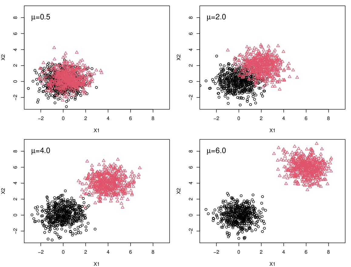
We simulated two bivariate normal distributions and , allowed to range from 0 to 6 in steps of 0.50 (selected to display the full range of the distance measures), and set where is the identity. See Figure 1 for an example of the simulated data.
True Distances. Results are provided in Figure 2 (solid black lines). and are nearly identical and increase linearly as the two clusters become farther apart. also increases linearly, however the true AB is not zero even for identical distributions. and are also nearly identical; they are highly sensitive to small changes when the clusters are overlapping but have limited sensitivity when clusters are further apart. In contrast, has limited sensitivity when cluster are overlapping but is highly sensitive when clusters are further apart.

Empirical Distances. Empirical distances are displayed by the dashed lines in Figure 2, with the colored points coded based on the ARI for that scenario. For all scenarios except the most highly overlapping (, poor cluster recovery), the estimated , , , and are accurate. In contrast, the estimated and performed poorly; they significantly underestimated the distance when cluster recovery was excellent.
3.2 Scenario 2: Bivariate Normal Clusters with Varying Scales
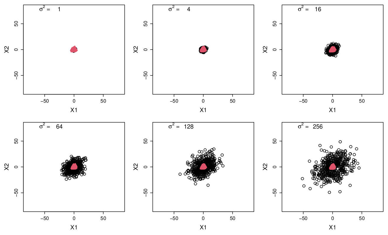
We simulated two bivariate normal distributions and where and are proportional to the identity matrix , with doubling among . See Figure 3 for an example of the simulated data.
True Distances. Results are provided in Figure 4 (solid black lines). , , and increase relatively linearly with larger differences in scale. and are more sensitive to small scale differences but less sensitive to large scale differences. is fixed at , which is expected because the means are identical.

Empirical Distances. Empirical distances are displayed by the dashed lines in Figure 4, with the colored points coded based on the ARI. Estimated is accurate across all scenarios, even with poor cluster recovery. Estimated and are accurate except for in the two most highly overlapping scenarios (, poor cluster recovery). Estimated , , and cannot cannot distinguish any differences across the scenarios, even when cluster recovery is excellent.
3.3 Scenario 3: MGH Distribution with Varying Rotation and Skewness
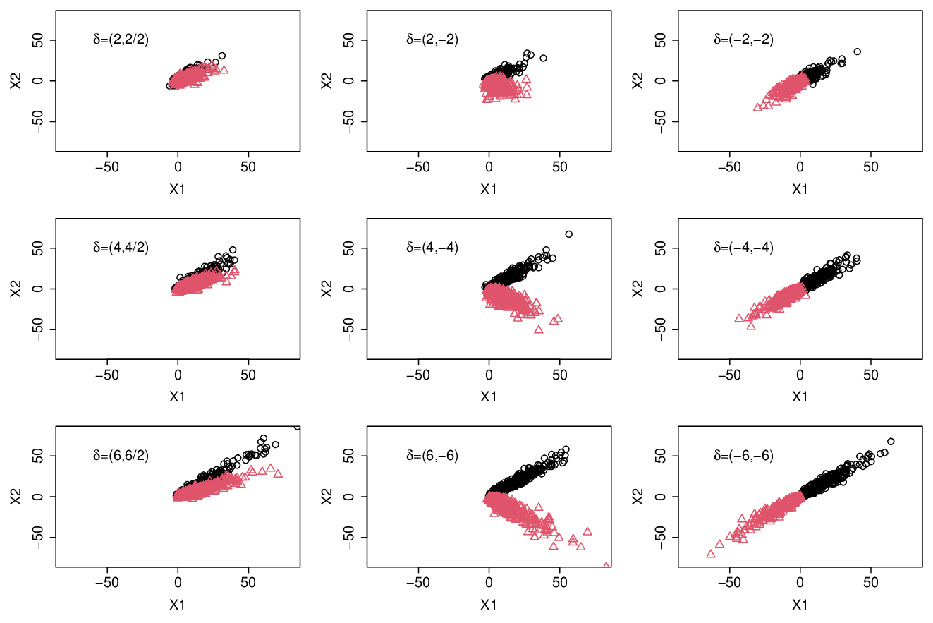
We simulated two clusters, each following a bivariate generalized hyperbolic distribution. The locations and scales of the two clusters were identical, such that and
with . Concentration parameters and were set to 1 for both clusters. For cluster 1 we set the magnitude and direction of skewness as , with . For cluster 2 we varied the skewness every around the circle coordinates with radius until the clusters were in opposite directions (180°) at . Example data are displayed in Figure 5.
True Distances. We first examined and across the various parameter combinations (Figure 6). and do not correspond well, especially in situations where the clusters are highly overlapping but not identical (e.g. ). (used to compute ) can have components whose sum can be negative. In the case of the MGH distribution, which has large observations with appreciable probability, these negative components can be extreme and pull the value lower. In contrast, by definition cannot have negative components within the square root, which ultimately results in a larger relative to . We only further consider within this Scenario.

The solid black lines in Figure 7 display the true distances across parameter combinations. Both and increase linearly as the second cluster moves clockwise around the circle to (a rotation from cluster 1). has two additional beneficial properties not observed with : (1) it increases with a higher magnitude of skewness and (2) it is when the two clusters are identical. and again perform similarly to one another. They are both sensitive to the smaller initial rotations but have limited sensitivity to changes in rotation past ( rotation). At , where the two clusters are identical, both and are appropriately ; they also both asymptotically approach as the rotation for cluster 2 nears (a rotation from cluster 1). displays limited change except for with the largest magnitude of skewness ().

Empirical Distances. Empirical distances are displayed by the dashed lines in Figure 7, with the colored points coded based on the ARI. over-estimates the distance when recovery is poor, but under-estimates the distance when recovery is good-to-moderate. and over-estimate the distance with rotation difference between clusters. With at least a rotation difference, and are relatively accurate; despite their general lack of sensitivity to changes in rotation within this range. drastically over-estimates smaller rotation differences, especially when . However, was surprisingly accurate with at least moderate cluster recovery and also increased somewhat linearly with added rotations. Finally, consistently over-estimated distances, especially in the scenarios corresponding to poor cluster recovery.
4 Application
Data from the Transdiagnostic Anxiety Spectrum study were collected by Peter Lang, Ph.D. and colleagues at the University of Florida Center for the Study of Emotion and Attention (MH082702; MH72850). The analytic sample employed here includes adults across eight different anxiety disorders plus major depressive disorder and healthy controls. Participants in this study listened to narratives varying in emotional imagery while five physiological responses were measured: Corrugator response (COR), orbicularis electromyography (ORB), startle reflex (STL), skin conductance response (SCR), and heart rate (HR). In this illustration we focus on identifying cross-diagnostic subtypes with similar physiological responses to pleasant imagery relative to neutral imagery. Measures were computed as the pleasant physiological response minus the neutral physiological response.
4.1 Selecting the Number of Clusters
Using R we fit both MVN (Mclust package) and MCGHD (MixGHD package) mixture models to the five physiological responses to pleasant versus neutral imagery, considering 1-5 clusters. For MVN we also considered the large array of covariance types that are available through the package. To select the optimal model for Mclust we selected the one that maximized the , which is conventional for this approach. To select the optimal model for MixGHD, we used a more nuanced approach because the models are more complex and have a much larger number of parameters to estimate. Therefore, we considered the Bayesian Information Criteria (BIC), Akaike Information Criterion (), and Integrated Complete-Data Likelihood (). We prioritized clustering solutions that maximized the and and/or which preceded a drop in ICL. We identified 3 MCGHD clusters using MixGHD and 4 MVN clusters using Mclust .
4.2 Cluster Characterization using Descriptive Statistics
We used descriptive statistics (median [Q1, Q3]) to summarize the physiological responses in each cluster (Table 4.2). We also used Kruskal-Wallis tests to determine whether the responses differed by cluster.
Based on the MVN mixture model solution, participants in have the strongest response to pleasant (vs. neutral) imagery on COR, ORB, STL, and HR, while participants in have the strongest response on SCR. Participants in clusters and have lower-moderate responses. SCR, HR, and ORB differed significantly across the four clusters identified using the MVN mixture model.
Based on the MCGHD mixture model solution, participants in have the strongest response on STL, SCR, and HR, participants in have the strongest response on COR and ORB, and participants in have lower responses. All five measures differed significantly across the three clusters identified using the MCGHD mixture model.
Median (Q1, Q3) of physiological characteristics by cluster. Startle Response Skin Conductance Response Heart Rate Corrugator Response Orbicularis Response Total (N=505) 1.53 (-1.29, 5.27) 0.00 (-0.00, 0.02) 0.39 (-0.72, 1.52) -0.05 (-0.37, 0.23) 0.52 (0.06, 1.19) MCGHD Mixture Model C1 (N=96) 4.00 (0.59, 8.20) 0.02 (0.00, 0.05) 1.92 (1.44, 2.99) 0.05 (-0.07, 0.27) 0.68 (0.31, 1.28) C2 (N=132) 0.97 (-0.71, 3.63) 0.00 (0.00, 0.01) 0.35 (-0.52, 1.15) 0.26 (-0.86, 1.06) 1.17 (0.39, 2.53) C3 (N=277) 1.17 (-2.58, 4.96) 0.00 (-0.01, 0.01) -0.16 (-1.15, 1.04) -0.13 (-0.41, 0.04) 0.25 (-0.02, 0.76) MVN Mixture Model C1 (N=226) 1.55 (-2.67, 6.20) 0.02 (-0.02, 0.04) 0.53 (-0.74, 1.74) -0.06 (-0.33, 0.14) 0.52 (0.08, 1.17) C2 (N=90) 0.59 (-1.32, 3.25) 0.00 (0.00, 0.01) 0.13 (-1.14, 1.08) 0.08 (-1.04, 0.98) 0.97 (0.03, 2.13) C3 (N=137) 1.81 (-0.43, 4.78) 0.00 (0.00, 0.01) 0.24 (-0.63, 1.26) -0.06 (-0.23, 0.08) 0.27 (-0.02, 0.55) C4 (N=52) 2.58 (-0.84, 10.88) 0.00 (-0.02, 0.04) 1.38 (-0.48, 2.63) 0.14 (-1.05, 1.53) 2.09 (0.59, 3.90)
4.3 Cluster Contour Plots
Figure 8 illustrates elliptical clusters generated using parameter estimates from the MVN mixture model. has a large scale and encompasses the other clusters, despite the relatively small sample size (). In contrast, has a very small scale relative to the other clusters. Perhaps as a result of these notable differences in scale, it is difficult to graphically distinguish mean differences between clusters.

Figure 9 illustrates the clusters generated using the parameter estimates from the MCGHD mixture model. Clusters are non-elliptical with differences in location, scale, and rotation. For example, in plots of COR vs. HR and ORB vs. HR, is rotated from and , and generally has higher HR levels than and . also has a larger scale on COR and ORB relative to the other clusters.

4.4 Distance Measures
Although summary statistics and plots important tools for cluster interpretation, they cannot succinctly summarize: (1) which clusters are most separate from other clusters within a given solution; or (2) whether the MVN or MCGHD solution suggests pairs of clusters that are more distinct. The proposed distance measures can fill these gaps. For each pair of clusters and each clustering approach (MCGHD, MVN), we computed four metrics previously considered in the simulation study (, , , , and ). However, we gave , , and more consideration because of the relatively poor performance of and in the simulation study. was not considered because its computation is not meaningful for the MCGHD model and it cannot distinguish differences in scale.
![[Uncaptioned image]](2206.11465v1/pln_mclust_ghd_distances_radial.png)
Distances between pairs of clusters. The top row reflects pairwise distances from the MVN model. The bottom row reflects pairwise distances from the MCGHD model.
The top row of plots in Figure 4.4 display pairwise cluster distances from the MVN model. All five metrics indicate that and have the greatest distance between them, and that is not particularly distinct from other clusters. , , and indicate that and are well-separated.
The bottom row of plots in Figure 4.4 displays pairwise cluster distances from the MCGHD model. The distances between each pair of clusters are relatively large when quantified by , , , and . There is some inconsistency regarding which specific pair has the largest distance, with , , , and indicating and have the largest distance, and indicating that and have the largest distance. Despite this incongruity, still emerges as the cluster that is most distinct from the other clusters.
When comparing each measure across MCGHD and MVN clustering solutions, distances between MCGHD clusters are overall larger; however some some specific pairwise distances in the MVN solution are also large (e.g., between and ). It is also noteworthy that provides a high level of sensitivity to distinguishing cluster differences among pairs, whereas and have limited ability to distinguish such differences. This is consistent with the simulation study results, which showed and are less sensitive to detecting differences between larger distances.
5 Discussion
Interpretation of a clustering solution is often the most challenging aspect of a cluster analysis. Metrics that aid in determining whether clusters are meaningfully distinct from one another can facilitate this process. Given the expanding field of finite mixture modeling with non-elliptical clusters, it is essential to consider metrics that accommodate flexible cluster shapes. Our review and simulation study provide insight regarding several such metrics.
The Wasserstein Distance (), Hellinger Distance (), and the Extended Jensen Shannon Distance () had good accuracy in the majority of simulation scenarios, as long as cluster recovery was moderate as indicated by the Adjusted Rand Index. and have the advantage of being bounded by and , a property that potentially allows for easier indexing of potential benchmarks for effect size. However, a caveat is that and flatten as they near 1 (e.g., ), which means that very small changes in value toward the upper bound may correspond to deceivingly large shifts in mean, rotation, or scale. In contrast, generally changed linearly, which enhances its interpretability. also appeared to be more sensitive to differences in scale and rotation than other metrics. For example, in Scenario 1 (mean differences between MVN clusters) the maximum was roughly , while in Scenarios 2 and 3 (differences in scale and rotation) the maximum was roughly times as large. This has important implications, as it suggests that will generally be larger between two clusters that differ in scale or rotation, relative to two clusters that differ in mean.
While and performed well in some simulation scenarios, other scenarios indicated their potential to be misleading when used for our specific questions. For example, they may may suggest cluster distances that are too large when cluster recovery is very poor, or too small even if cluster recovery is excellent. It is also important to emphasize that , , and are not able to distinguish differences in scale, which is a major limitation of these metrics if the interest is in quantify distances between more flexible cluster shapes.
An important observation across both the simulation and application is that the choice of a different distance measure can lead to a different conclusion regarding which clusters have the greatest separation between them. For this reason, we recommend using multiple metrics (e.g., , , ) and expect that the clusters with the greatest separation will be observed across multiple metrics. This phenomenon is common in mixture modeling. For example, the AIC, BIC, and ICL are commonly used together although they can all suggest different results. In clustering more broadly, many different approaches can be used to suggest the number of clusters, with a wide range of potential results.
There are limitations and caveats to our work to be considered. First, we have not identified which levels of each metric might be considered notable in an applied context. Linking the metrics to ballpark estimates of “small”, “medium” or “large” effect sizes would further promote their utility (Sullivan and Feinn 2012; Cohen 1990). Second, the probability-based distance measures (, , ) as we have presented them are only relevant for clusters identified through mixture modeling or data simulation because they require known or estimated parameters. We chose to focus on mixture modeling because it facilitates identification of non-elliptical clusters, an important and emerging area of health research. However, a consequence of this focus is that the distances as proposed can not be directly applied to clusters identified through approaches that only output cluster membership (e.g., k-means algorithm).
In future research, it may be useful to extend our work to non-model-based clustering approaches. may be amenable to this adaptation because it is possible to compute it using the observed data within each cluster, rather than estimated parameters. Recent advances advancements to may also facilitate measuring distances between clusters with different sample sizes (Séjourné et al. 2019). Along these same lines, there are also existing approaches that allow for empirical estimation of and . We did not use empirical estimation because of the practical concern of small (and unequal) sample sizes, and the impact this might have on estimation of distance metrics. However, future work in this area would facilitate the use of distance measures for a wider range of clustering methods.
Disclosure statement
MLW is a consultant for Noctem, Sleep Number Bed, and Health Rhythms, unrelated to this work.
Funding
This work was supported by the National Institute of Mental Health under grant number R03MH116478.
References
- Rub (1998) 1998. A metric for distributions with applications to image databases; Jan.
- Aitkin et al. (1981) Aitkin M, Anderson D, Hinde J. 1981. Statistical modelling of data on teaching styles (with discussion). Journal of the Royal Statistical Society, Series B:419–461.
- Bhattacharyya (1943) Bhattacharyya A. 1943. On a measure of divergence between two statistical populations defined by their probability distributions. Bulletin of the Calcutta Mathematical Society. 35:99–109.
- Browne and McNicholas (2015) Browne R, McNicholas P. 2015. A mixture of generalized hyperbolic distributions. Canadian Journal of Statistics. 43(2):176–198.
- C.L. (1972) CL M. 1972. A note on asymptotic joint normality. Annals of Mathematical Statistics. 43(2):508–515.
- Cohen (1990) Cohen J. 1990. Things i have learned (so far). American Psychologist. 45:1304–1312.
- Del Guidice (2017) Del Guidice M. 2017. Heterogeneity coefficients for mahalanobis’ d as a multivariate effect size. Multivariate Behavioral Research. 52:216–221.
- Franczak et al. (2014) Franczak BC, Browne RP, McNicholas PD. 2014. Mixtures of shifted asymmetriclaplace distributions. IEEE Trans Pattern Anal Mach Intell. 36:1149–1157.
- Hadi (2022) Hadi A. 2022. A new distance between multivariate clusters of varying locations, elliptical shapes, and directions. Pattern Recognition. 129:108780.
- Hennig (2014) Hennig C. 2014. How many bee species? a case study in determining the number of clusters. In: Spiliopoulou M, Schmidt-Thieme L, Janning R, editors. Data Analysis, Machine Learning and Knowledge Discovery; Cham. Springer International Publishing. p. 41–49.
- Hennig (2020) Hennig C. 2020. fpc: Flexible procedures for clustering. R package version 2.2-9; Available from: https://CRAN.R-project.org/package=fpc.
- Kullback and Leibler (1951) Kullback S, Leibler R. 1951. On information and sufficiency. Annals of Mathematical Statistics. 22(1):79–86.
- Lee and McLachlan (2013) Lee S, McLachlan G. 2013. On mixtures of skew normal and skew t-distributions. Advances in Data Analysis and Classification. 7(3):241–266.
- Nielson (2020) Nielson F. 2020. Non-negative monte carlo estimation of f-divergences. Tokyo, Japan: Sony Computer Science Laboratories, Inc.
- Pyne et al. (2009) Pyne S, Hu X, Wang K, Rossin E, Lin TI, Maier LM, Baecher-Allan C, McLachlan GJ, Tamayo P, Hafler DA, et al. 2009. Automated high-dimensional flow cytometric data analysis. Proceedings of the National Academy of Sciences. 106(21):8519–8524.
- R Core Team (2020) R Core Team. 2020. R: A language and environment for statistical computing. Vienna, Austria: R Foundation for Statistical Computing. Available from: https://www.R-project.org/.
- Rachev (1984) Rachev ST. 1984. The monge-kantorovich mass transference problem and its stochastic applications. Theory of Probability and its Applications:647–676.
- Rubner et al. (1998) Rubner Y, Tomasi C, Guibas LJ. 1998. The earth mover’s distance as a metric for image retrieval. Department of Computer Science, Stanford University. Report No: Technical Report STAN-CS-TN-98-86.
- Sahu et al. (2003) Sahu SK, Dey DK, Branco MD. 2003. A new class of multivariate skew distributions with applications to bayesian regression models. Canadian Journal of Statistics. 31(2):129–150.
- Schuhmacher et al. (2020) Schuhmacher D, Bähre B, Gottschlich C, Hartmann V, Heinemann F, Schmitzer B. 2020. transport: Computation of optimal transport plans and wasserstein distances. R package version 0.12-2; Available from: https://cran.r-project.org/package=transport.
- Scrucca et al. (2016) Scrucca L, Fop M, Murphy TB, Raftery AE. 2016. mclust 5: clustering, classification and density estimation using Gaussian finite mixture models. The R Journal. 8(1):289–317. Available from: https://doi.org/10.32614/RJ-2016-021.
- Steinley (2004) Steinley D. 2004. Properties of the hubert-arabie adjusted rand index. Psychological Methods. 9(3):386–396.
- Sullivan and Feinn (2012) Sullivan G, Feinn R. 2012. Using effect size-or why the p value is not enough. Journal of Graduate Medical Education. 4(3):279–282.
- Séjourné et al. (2019) Séjourné T, Feydy J, Vialard F, Trouvé A, Peyré G. 2019. Sinkhorn divergences for unbalanced optimal transport. arXiv:191012958.
- Tortora et al. (2021) Tortora C, ElSherbiny RPBA, Franczak BC, , McNicholas PD. 2021. Model-based clustering, classification, and discriminant analysis using the generalized hyperbolic distribution: Mixghd r package. Journal of Statistical Software. 98(1):1,24.
- Tortora et al. (2019) Tortora C, Franczak BC, Browne RP, McNicholas PD. 2019. A mixture of coalesced generalized hyperbolic distributions. Journal of Classification. 36(1):26–57.