An accurate and efficient scheme for function extensions on smooth domains

Charles L. Epstein Thanks: Center for Computational Mathematics, Flatiron Institute, Simons Foundation, New York, New York 10010 (cepstein@flatironinstitute.org). Fredrik Fryklund Thanks: Courant Institute of Mathematical Sciences, New York University, New York, New York 10012 (nf2235@nyu.edu). Shidong Jiang Thanks: Center for Computational Mathematics, Flatiron Institute, Simons Foundation, New York, New York 10010 (sjiang@flatironinstitute.org).

Abstract

A new scheme is proposed to construct an $n$ -times differentiable function extension of an $n$ -times differentiable function defined on a smooth domain, $D,$ in $d$ -dimensions. The extension scheme relies on an explicit formula consisting of a linear combination of $n+1$ function values in $D,$ which extends the function along directions normal to the boundary. Smoothness tangent to the boundary is automatic. The performance of the scheme is illustrated by using function extension as a step in a numerical solver for the inhomogeneous Poisson equation on multiply connected domains with complex geometry in two and three dimensions. We show that the modest additional work needed to do function extension leads to considerably more accurate solutions of the partial differential equation.

keywords

function extension, Vandermonde matrix, Chebyshev polynomial, complex geometry, smooth domain, elliptic partial differential equations

AMS

31B10, 65N80, 65T99

1 Introduction

In a classic paper by Robert Seeley [19], a simple formula is given for the ${\mathcal{C}}^{\infty}$ extension of a ${\mathcal{C}}^{\infty}$ function defined in a half space. To be more precise, let $y\in\mathbb{R}^{d-1}$ , $x\in\mathbb{R}^{1}$ , ${\mathbb{R}}^{d}_{+}=\mathbb{R}^{d-1}\times\{x\geq 0\}$ , then ${\mathcal{C}}^{\infty}({\mathbb{R}}^{d}_{+})$ consists of infinitely differentiable functions defined in ${\mathbb{R}}^{d-1}\times(0,\infty)$ whose derivatives have continuous limits as $x\rightarrow 0^{+}$ . For $x<0$ , define the extended function

E_{\infty}[f](y,x)=\sum_{j=0}^{\infty}w_{j}f(y,-t_{j}x)\phi(-t_{j}x),

(1)

where $\{t_{j}\}\subset(0,\infty)$ is an unbounded, strictly increasing sequence, and $\phi$ is a ${\mathcal{C}}^{\infty}$ window function on $\mathbb{R}^{1}$ with $\phi(x)=1$ for $0\leq x\leq 1$ , and $\phi(x)=0$ for $x\geq 2$ . For any $x<0,$ the sum in eq. 1 is finite and therefore $E_{\infty}[f]$ has the same smoothness as the original function $f.$ In order to ensure the smoothness of the extension across the boundary, one needs to require that the values of $E_{\infty}[f]$ and $f$ and all of their derivatives match at $x=0$ . This leads to the following infinite system of linear equations for $\{w_{j}\}$

\sum_{j=0}^{\infty}w_{j}t_{j}^{i}=(-1)^{i},\qquad i=0,1,\cdots,

(2)

i.e., the weight vector $w$ is the solution to an infinite Vandermonde system when the node vector $t=(t_{0},t_{1},\dots)$ is given. Using $t_{j}=2^{j}$ , Seeley showed that $\sum_{j=0}^{\infty}|w_{j}||t_{j}|^{i}<\infty$ for all $i\geq 0$ . Thus, the extension operator $E_{\infty}$ is actually a continuous linear operator from $C^{\infty}(\mathbb{R}^{d}_{+})$ to $C^{\infty}(\mathbb{R}^{d})$ .

Here we examine the extension formula eq. 1 from the perspective of numerical computation. Function extensions have broad applications in numerical analysis and scientific computing, especially to boundary value problems for partial differential equations where the boundary does not have simple geometry. Most existing numerical schemes rely on a data fitting procedure using a choice of basis functions such as Fourier series, polynomials, radial basis functions, etc. (see, for example, [2, 8, 9, 10, 11, 15, 23, 24]). The data fitting procedure is usually carried out on a volume grid to ensure the smoothness of the extended function in all variables, which is expensive for problems in two and higher dimensions. In [8] a method is introduced that extends along the normal direction using Fourier continuation. There is also the active penalty method [20], where an extension is created by using a set of basis functions that give global regularity $C^{k}$ , once boundary data and derivatives of order $k$ have been matched at the boundary. Observe that all of these schemes depend on the original data linearly, regardless of the basis functions chosen to fit the data; that is, the extension operator is a linear operator.

As opposed to function extension, there is the method of function intension [22]. The source density is represented on a uniform Cartesian grid in the interior of the given computational domain, combined with a conforming mesh in a tubular neighborhood of the boundary. The Poisson equation is solved in each region, followed by enforcing consistency of the solution, across the interface of the interior of the domain and the tubular neighborhood, by solving a boundary integral equation. Another method that relies on volumetric domain decomposition is [1], which is compatible with standard meshing software.

For applications to numerical analysis it is more appropriate to consider the finitely differentiable analogue of $E_{\infty},$ given by

E_{n}[f](y,x)=\sum_{j=0}^{n}w_{j}f(y,-t_{j}x)\phi(-t_{j}x),

(3)

where now we have the finite Vandermonde system:

\sum_{j=0}^{n}w_{j}t_{j}^{i}=(-1)^{i},\qquad i=0,1,\cdots,n.

(4)

A nice feature of the extension formulæ eq. 1 and eq. 3 is that the extension acts along one direction only, while the smoothness in the other directions is automatically guaranteed by construction. This feature can be extended to domains $D\subset{\mathbb{R}}^{d},$ with $\partial D$ a smooth embedded hypersurface. For $y\in\partial D,$ let $\nu_{y}$ denote the outer unit normal vector to $\partial D$ at $y.$ The tubular neighborhood theorem, see [7], ensures that for some $\epsilon>0$ the map from $\partial D\times(-\epsilon,\epsilon)$ given by

(y,x)\mapsto y+x\nu_{y}

(5)

is a diffeomorphism onto its image. For such a domain $D\subset\mathbb{R}^{d}$ , we can extend the definition of $E_{n}$ by setting

E_{n}[f](y+x\nu_{y})=\sum_{j=0}^{n}w_{j}f(y-t_{j}x\nu_{y}),

(6)

where $y$ is a point on $\partial D$ . The window function is dropped for now, but will be needed in some applications.

Once again, $E_{n}[f]$ has the same order of smoothness as $f$ in $\overline{D}^{c}$ and along the tangential directions on $\partial D$ by construction. Thus, one only needs to ensure the continuity of the function and its normal derivatives up to order $n$ on $\partial D$ in order for the extension to be in ${\mathcal{C}}^{n}$ in a small neighborhood of $D$ . This leads to the following $(n+1)\times(n+1)$ Vandermonde linear system for the nodes and weights

\begin{bmatrix}1&1&\cdots&1\\ t_{0}&t_{1}&\cdots&t_{n}\\ \vdots&\vdots&\cdots&\vdots\\ t_{0}^{n}&t_{2}^{n}&\cdots&t_{n}^{n}\end{bmatrix}\begin{bmatrix}w_{0}\\ w_{1}\\ \vdots\\ w_{n}\end{bmatrix}=\begin{bmatrix}1\\ -1\\ \vdots\\ (-1)^{n}\end{bmatrix},

(7)

which we write as $Aw=c$ for short. In general such systems are very poorly conditioned, but, as we show in section 2, the solution to this equation can be found explicitly, without recourse to numerical linear algebra.

Another very nice feature of this approach is that the nodes and weights are independent of the domain, $D.$ By the nature of the extension operator, we need to have $t_{j}\geq 0$ for $j=0,\ldots,n$ and without loss of generality, we assume that they are arranged in increasing order, i.e., $0\leq t_{0}<t_{1}<\cdots<t_{n}$ . The extension $E_{n}[f]$ is then obtained by simply evaluating the sums in eq. 6. While this does not require the solution of any equations, it generally requires $f$ to be interpolated to the values of the arguments $\{y-t_{j}x\nu_{y}:\>j=0,\dots,n\}$ that appear in the sum.

The paper is organized as follows. In section 2, we present the main theoretical result. Section 3 discusses certain numerical issues associated with the application of our function extension scheme to solving elliptic partial differential equations. Numerical results in one, two, and three dimensions are shown in section 4.

2 Main theoretical result

The main theoretical result of this paper is theorem 13, which gives the optimal nodes and weights of the function extension formula eq. 6.

2.1 Solution to the Vandermonde system

It is well known that Vandermonde matrices are ill-conditioned (as is familiar in the problem of function extrapolation). In [12], it is shown that the condition number (in the maximum norm) of the Vandermonde matrix is bounded from below by $(n+1)2^{n}$ when all nodes are non-negative. If the weights are calculated by solving eq. 7 numerically, then the condition number of the Vandermonde matrix will affect the accuracy of the weights. However, eq. 7 can be solved analytically by an elementary method, which we now present. Denote by $B$ the inverse of the matrix $A$ . We then have

\sum_{j=0}^{n}b_{ij}t_{k}^{j}=\delta_{ik}.

(8)

Consider the polynomial $p_{i}(x)=\sum_{j=0}^{n}b_{ij}x^{j}$ . Then eq. 8 is equivalent to

p_{i}(t_{k})=\delta_{ik}.

(9)

Recall that the Lagrange basis functions $\{l_{i}(x)\}$ for interpolation through the nodes $\{t_{k},k=0,\cdots,n\}$ are given by

l_{i}(x)=\prod_{m=0,m\neq i}^{n}\frac{x-t_{m}}{t_{i}-t_{m}},

(10)

and the interpolant is then

Q(x)=\sum_{i=0}^{n}f_{i}l_{i}(x).

(11)

It is straightforward to check that $l_{i}$ satisfies the condition eq. 9. Thus,

p_{i}(x)=l_{i}(x),

(12)

and

	$\displaystyle w_{i}$	$\displaystyle=\sum_{j=0}^{n}b_{ij}(-1)^{j}=p_{i}(-1)=l_{i}(-1)$		(13)
		$\displaystyle=(-1)^{i}\prod_{m=0}^{i-1}\frac{1+t_{m}}{t_{i}-t_{m}}\cdot\prod_{m=i+1}^{n}\frac{1+t_{m}}{t_{m}-t_{i}}.$		(13)

That is, $w_{i}$ is the value of the $i$ th Lagrange basis function evaluated at $-1$ .

2.2 Choice of optimal interpolation nodes

To fix our discussion, let us now assume that the ${\mathcal{C}}^{n}$ function, $f,$ is defined in the interval $[0,a],$ and we extend $f$ to $[-1,0],$ which means that the nodes $\{t_{i}\}\subset[0,a]$ as well. $E_{n}$ extends functions in ${\mathcal{C}}^{n}([0,a])$ to functions in ${\mathcal{C}}^{n}([-1,a]);$ we see that

\|E_{n}(f)\|_{L^{\infty}([-1,0])}\leq\|w\|_{1}\|f\|_{L^{\infty}([0,a])},

(14)

where

\|w\|_{1}=\sum_{i=0}^{n}|w_{i}|.

(15)

Hence a good measure of the “quality” of the extension operator given by eq. 6 is the $\ell^{1}$ -norm of the weights $\{w_{j}\}.$ This norm, $\|w\|_{1},$ is determined by the interpolation nodes $\{t_{i}\}$ explicitly via the formula eq. 13. We would therefore like to choose the interpolation nodes $t_{i}\in[0,a]$ such that $\|w\|_{1}$ is minimized. While we are not explicitly controlling the norms of the derivatives $\|\partial_{x}^{l}E_{n}[f]\|_{L^{\infty}}([-1,0]),$ for $l=1,\dots,n,$ below we see that, for the nodes and weights that minimize $\|w\|_{1},$ these norms behave like $a^{l}\|w\|_{1}\|\partial_{x}^{l}f\|_{L^{\infty}([0,a])}.$ In applications $a\approx 2,n\leq 10,$ so this is a very moderate rate of growth.

Combining eq. 11 and eq. 13, we obtain

$\displaystyle\\|w\\|_{1}$	$\displaystyle=\sum_{i=0}^{n}\|w_{i}\|$	(16)
	$\displaystyle=\sum_{i=0}^{n}(-1)^{i}l_{i}(-1)$
	$\displaystyle=P(-1),$

where $P(x)=\sum_{i=0}^{n}(-1)^{i}l_{i}(x)$ .

Definition 1.

A polynomial $P$ is said to satisfy the equi-oscillation property of modulus $1$ on $[0,a]$ if there exist $t_{i}$ with $0\leq t_{0}<t_{1}<\cdots<t_{n}\leq a$ such that $P(t_{i})=(-1)^{i}$ for $i=0,\ldots,n$ .

Lemma 2.

If $P(x)$ is a polynomial of degree $n,$ satisfying the equi-oscillation property of modulus $1$ , then its $n$ roots $x_{i}$ ( $i=1,\cdots,n$ ) satisfy the property $t_{0}<x_{1}<t_{1}<x_{2}<t_{2}<\cdots<x_{n}<t_{n}$ .

Proof.

This follows from the intermediate value theorem and the fact that the signs of the values $\{P(t_{0}),P(t_{1}),\dots,P(t_{n})\}$ alternate.

Lemma 3.

If $P(x)$ is a polynomial of degree $n,$ satisfying the equi-oscillation property of modulus $1$ , then $P(x)>0$ decreases monotonically for $x<t_{0}$ .

Proof.

This follows from lemma 2 and the fact that $P(t_{0})=1$ . That is, $P(x)=c\prod_{i=1}^{n}(x_{i}-x)$ for some $c>0$ .

It is easy to see that the choice of optimal interpolation nodes for the purpose of function extension is equivalent to the following problem:
Find the minimal value of $P(-1)$ among all polynomials of degree at most $n$ that satisfy the equi-oscillation property of modulus $1$ on $[0,a]$ .

Denote the minimal value by $m_{a}$ , the corresponding polynomial by $p^{\ast}(x)$ , and the associated nodes by $\{t_{j}^{\ast}\}$ , respectively. In the following lemmas we give the properties of the optimal nodes and $p^{\ast}$ itself.

Lemma 4.

$t_{0}^{\ast}=0$ .

Proof.

Suppose $t_{0}^{\ast}>0$ . Then $q(x)=p^{\ast}(x+t_{0}^{\ast})$ satisfies the alternating property $q(t_{i}^{\ast}-t_{0}^{\ast})=p^{\ast}(t_{i}^{\ast})=(-1)^{i}$ . Furthermore, $q(-1)=p^{\ast}(-1+t_{0}^{\ast})<p^{\ast}(-1)$ by lemma 3, which leads to a contradiction.

Lemma 5.

If $n>0$ , then $t_{n}^{\ast}=a$ .

Proof.

Suppose $t_{n}^{\ast}<a$ . Consider the polynomial $q(x)$ , which is obtained by replacing $t_{n}^{\ast}$ by $a$ and keep all other nodes unchanged. We claim that $q(-1)<p^{\ast}(-1)$ . This can be seen from eq. 13, eq. 16, and the facts that both $\frac{1}{t_{n}-t_{m}}$ and $\frac{1+t_{n}}{t_{n}-t_{i}}=1+\frac{1+t_{i}}{t_{n}-t_{i}}$ decrease as $t_{n}$ increases. Hence the contradiction.

Lemma 6.

If $a_{1}>a_{2}$ , then $m_{a_{1}}<m_{a_{2}}$ .

Proof.

By the definition of the problem, we have $m_{a_{1}}\leq m_{a_{2}}$ since the space of allowable functions becomes larger as $a$ increases. The strict inequality is achieved by lemma 5.

Lemma 7.

$|p^{\ast}(x)|\leq 1$ for $x\in(0,a)$ .

Proof.

Suppose first that $p^{\ast}(t^{\circ})>1$ at some point $t^{\circ}\in(0,a)$ . Let $t_{j}^{\ast}$ be the closest node to $t^{\circ}$ such that $p^{\ast}(t^{\ast}_{j})=1$ . It is clear that $j$ has to be even and $t^{\circ}<t_{j+1}^{\ast}$ by the alternating property. Consider the polynomial $q(x)$ which is obtained by replacing $t_{j}^{\ast}$ with $t^{\circ}$ . Then $p^{\ast}(t_{i}^{\ast})-q(t^{\ast}_{i})=0$ for $i\neq j$ . That is,

p^{\ast}(x)-q(x)=c\prod_{i=0}^{j-1}(x-t^{\ast}_{i})\cdot\prod_{i=j+1}^{n}(t^{\ast}_{i}-x),

(17)

Furthermore, since $p^{\ast}(t^{\circ})-q(t^{\circ})=p^{\ast}(t^{\circ})-1>0$ , we must have $c>0$ . It then follows that

	$\displaystyle p^{\ast}(-1)-q(-1)$	$\displaystyle=c\prod_{i=0}^{j-1}(-1-t^{\ast}_{i})\cdot\prod_{i=j+1}^{n}(t^{\ast}_{i}+1)$		(18)
		$\displaystyle=c\prod_{i=0}^{j-1}(1+t^{\ast}_{i})\cdot\prod_{i=j+1}^{n}(t^{\ast}_{i}+1)>0$		(18)

due to the facts that $c>0$ and $j$ is even. Hence the contradiction.

Suppose that $p^{\ast}(t^{\circ})<-1$ . Then a similar argument leads to eq. 18 again by the facts that $c<0$ and $j$ is odd.

Lemma 8.

$|p^{\ast}(x)|<1$ for $x\in(0,a)$ and $x\neq t_{i}$ , $i=0,1,\ldots,n$ .

Proof.

This follows from lemma 7, since otherwise there must be a point at which $|p^{\ast}|$ is greater than $1$ .

Lemma 9.

$p^{\ast\prime}(t^{\ast}_{i})=0$ for $i=1,\ldots,n-1$ .

Proof.

By lemma 7 and lemma 8, $p^{\ast}(x)$ achieves its interior extreme values at $t^{\ast}_{i}$ . Hence, its first derivative vanishes at those interior nodes.

The following lemma is key to the uniqueness.

Lemma 10.

If $p_{1}(x)$ and $p_{2}(x)$ satisfy the equi-oscillation property of modulus $1$ on $[0,a]$ and $|p_{1}(x)|\leq 1$ , $|p_{2}(x)|\leq 1$ , then $p_{1}(x)\equiv p_{2}(x)$ .

Proof.

Suppose that $p_{1}$ is not identically equal to $p_{2}$ . Then there exists a point $\xi<0$ such that $p_{1}(\xi)\neq p_{2}(\xi)>0$ . Without loss of generality, assume that $0<p_{1}(\xi)<p_{2}(\xi)$ . Consider the polynomial

q(x)=p_{1}(x)-\frac{p_{1}(\xi)}{p_{2}(\xi)}p_{2}(x).

(19)

By construction, $q(\xi)=0$ . Furthermore,

\left|p_{2}(x)\frac{p_{1}(\xi)}{p_{2}(\xi)}\right|<1,\quad x\in[0,a],

(20)

since $p_{1}(\xi)<p_{2}(\xi)$ and $|p_{2}(x)|\leq 1$ for $x\in[0,a]$ . Thus, $q$ has the same signs as $p_{1}$ at its equi-oscillation nodes. By the intermediate value theorem, $q$ has $n$ zeros on $(0,a)$ . Together with the zero at $\xi$ , $q$ has $n+1$ zeros. Since $q$ is a polynomial of degree at most $n$ , $q$ has to be identically equal to zero everywhere, which leads to a contradiction.

Using these results we can now give an explicit formula for $p^{\ast}$ and $\{t_{j}^{\ast}\}:$

Theorem 11.

$p^{\ast}$ is unique and $p^{\ast}(x)=T_{n}(1-2x/a)$ , where $T_{n}$ is the Chebyshev polynomial of degree $n$ .

Proof.

The uniqueness follows from lemma 10 and the existence follows from explicit construction. Namely, it is straightforward to check that $T_{n}(1-2x/a)$ satisfies the equi-oscillation property of modulus $1$ and $|T_{n}(1-2x/a)|\leq 1$ on $[0,a]$ .

Since we only used the fact that $-1$ is outside the interval $[0,a]$ in our proofs and $[0,a]$ can be translated to any interval $[a,b]$ , we actually showed the following statement is true.

Corollary 12.

Suppose that $p(x)$ is a polynomial of degree at most $n$ satisfying the property $p(t_{i})=(-1)^{i}$ or $p(t_{i})=(-1)^{i+1}$ for $a\leq t_{0}<t_{1}<\ldots<t_{n}\leq b$ . Then

|p(x)|\geq\left|T_{n}\left(\frac{2}{b-a}\left(x-\frac{a+b}{2}\right)\right)\right|,\qquad x\notin[a,b].

(21)

In other words, the translated and rescaled Chebyshev polynomials have the least growth outside $[a,b]$ among all polynomials with the equi-oscillation property of modulus $1$ on $[a,b]$ . This should be compared to the fact, which appears as Theorem 1.10 in [18], that among polynomials $p$ of degree $n,$ with sup-norm 1 on $[-1,1],$ the Chebyshev polynomial $T_{n}$ has the following extremal properties: for any $x_{0}\notin(-1,1),$ and $0\leq k\leq n,$

|p^{[k]}(x_{0})|\leq|T^{[k]}_{n}(x_{0})|.

(22)

Using the explicit expressions of $T_{n}$

T_{n}(x)=\left\{\begin{aligned} &\cos(n\arccos(x)),\quad|x|\leq 1\\ &\frac{1}{2}\left(\left(x-\sqrt{x^{2}-1}\right)^{n}+\left(x+\sqrt{x^{2}-1}\right)^{n}\right),\quad|x|\geq 1,\end{aligned}\right.

(23)

We may calculate the optimal weights explicitly. Recall that $T_{n}(\cos\frac{i\pi}{n})=(-1)^{i};$ consider the function

\phi(x)=\prod_{i=0}^{n}(x-t_{i}).

(24)

Then

l_{i}(x)=\frac{\phi(x)}{(x-t_{i})\phi^{\prime}(t_{i})},

(25)

and

w^{\ast}_{i}=l_{i}^{\ast}(-1)=-\frac{\phi^{\ast}(-1)}{(1+t_{i})\phi^{\ast\prime}(t_{i})}.

(26)

We first work on the standard interval $[-1,1]$ . By lemma 9, the $n-1$ interior nodes are the zeros of $T^{\prime}_{n}(x)$ . Thus, $\phi(x)=c(x^{2}-1)T^{\prime}_{n}(x)$ for the interval $[-1,1]$ . Back to $[0,a]$ , we have

\phi^{\ast}(x)=x(x-a)T^{\prime}_{n}(2x/a-1),

(27)

and

\phi^{\ast\prime}(x)=\frac{2}{a}x(x-a)T^{\prime\prime}_{n}(2x/a-1)+(2x-a)T^{\prime}_{n}(2x/a-1),

(28)

where the irrelevant constant $c$ is dropped.

Theorem 13.

The optimal nodes on $[0,a]$ for function extension formula eq. 6 are Chebyshev nodes of the second kind shifted and scaled to the interval $[0,a]$ :

t^{\ast}_{i}=\frac{a}{2}\left(1-\cos\left(\frac{i\pi}{n}\right)\right),\quad i=0,\ldots,n.

(29)

And the associated optimal weights are

w^{\ast}_{i}=(-1)^{i}\frac{C_{n}(a)}{(1+\delta_{i0}+\delta_{in})na(1+t_{i}^{\ast})},\quad i=0,\ldots,n,

(30)

where

C_{n}(a)=\frac{1+a}{\sqrt{x_{0}^{2}-1}}\left(\left(x_{0}+\sqrt{x_{0}^{2}-1}\right)^{n}-\left(x_{0}-\sqrt{x_{0}^{2}-1}\right)^{n}\right),\quad x_{0}=1+\frac{2}{a}.

(31)

Finally, the $l_{1}$ norm of the associated optimal weights is

	$\displaystyle\\|w^{\ast}\\|_{1}$	$\displaystyle=\sum_{i=0}^{n}\|w^{\ast}_{i}\|=T_{n}(1+2/a)$		(32)
		$\displaystyle=\frac{1}{2}\left(\left(1+\frac{2}{a}-2\sqrt{\frac{1}{a}+\frac{1}{a^{2}}}\right)^{n}+\left(1+\frac{2}{a}+2\sqrt{\frac{1}{a}+\frac{1}{a^{2}}}\right)^{n}\right).$		(32)

The function extension is, as expected, exponentially ill-conditioned. As $a$ increases, the condition number decreases, due to the fact that $-1$ is relatively closer to the origin with respect to the interval $[0,a]$ ; for $a>1$ the condition number is approximately $e^{\frac{2n(\sqrt{a}+1)}{a}}.$ Since the extension formula eq. 6 only imposes the minimal conditions to ensure ${\mathcal{C}}^{n}$ continuity across the boundary, it seems quite reasonable that eq. 32 can be viewed as the intrinsic condition number of any linear function extension scheme.

The formula for $E_{n}[f]$ can be differentiated to give

\partial_{x}^{l}E_{n}[f](x)=\sum_{j=0}^{n}(-t_{j})^{l}w_{j}f^{[l]}(-t_{j}x),

(33)

and therefore

|\partial_{x}^{l}E_{n}[f](x)|\leq\left[\sum_{j=0}^{n}t_{j}^{l}|w_{j}|\right]\|f^{[l]}\|_{L^{\infty}([0,a])},\text{ with }x\in[-1,0].

(34)

For the optimal weights we see that

\sum_{j=0}^{n}t^{*l}_{j}|w^{*}_{j}|\leq a^{l}\|w^{*}\|_{1}\frac{\sum_{j=0}^{n}\frac{\left(\frac{1}{2}(1-\cos\left(\frac{\pi j}{n}\right))\right)^{l}}{(1+t_{j}^{*})(1+\delta_{j0}+\delta_{jn})}}{\sum_{j=0}^{n}\frac{1}{(1+t_{j}^{*})(1+\delta_{j0}+\delta_{jn})}}

(35)

The ratio of sums is certainly less than 1, but also bounded below by $1/2(1+a)(n+1).$

As $n$ gets large, the numerator and denominator in eq. 35 can be seen as $n/\pi$ times the trapezoidal approximations to the integrals

\int_{0}^{\pi}\frac{\left[\frac{1}{2}(1-\cos x)\right]^{l}dx}{1+\frac{a}{2}(1-\cos x)}\text{ and }\int_{0}^{\pi}\frac{dx}{1+\frac{a}{2}(1-\cos x)},

(36)

respectively. Using contour integration to evaluate these integrals one can show that the denominator is approximated by $\frac{n}{\sqrt{1+a}}$ and the numerator by

\frac{n}{a2^{2(l-2)}}\sum_{j=0}^{l-1}\left(\begin{matrix}2(l-j-1)\\ l-j-1\end{matrix}\right)\left(\frac{-4}{a}\right)^{j}+8(-1)^{l+1}\frac{n}{a^{l}\sqrt{1+a}}.

(37)

Clearly, as $a$ grows, the $j=0$ term dominates the numerator, and therefore we have the estimate

\sum_{j=0}^{n}t^{*l}_{j}|w^{*}_{j}|\leq C_{l}\frac{1}{2^{2l}}\left(\begin{matrix}2(l-1)\\ l-1\end{matrix}\right)a^{l-\frac{1}{2}},

(38)

where $C_{l}$ is uniformly bounded as a function of $a,l,n.$

Table 1: Condition number of function extension formula eq. 6 in

l_{1}

norm. The first row lists the order of the function extension. The first column lists the size of the interval.

	$2$	$3$	$4$	$5$	$6$	$7$	$8$
$0.15$	$409.9$	$11\,735.8$	$336\,017$	$9\,620\,746$	$275\,458\,698$	$7\,886\,861\,923$	$225\,814\,583\,082$
$0.25$	$161.0$	$2889.0$	$51\,841$	$930\,249$	$16\,692\,641$	$299\,537\,289$	$5\,374\,978\,561$
$0.5$	$49.0$	$485.0$	$4801$	$47\,525$	$470\,449$	$4\,656\,965$	$46\,099\,201$
$1$	$17.0$	$99.0$	$577$	$3363$	$19\,601$	$114\,243$	$665\,857$
$2$	$7.0$	$26.0$	$97$	$362$	$1351$	$5042$	$18\,817$
$4$	$3.5$	$9.0$	$24$	$62$	$161$	$422$	$1104$

3 Numerical algorithms

3.1 Window function

Table 1 lists condition numbers of the function extension formula eq. 6, where the first row lists the extension order $n$ , and the first column lists the size of the interval, $a,$ where $f$ is defined. We observe that the condition numbers do increase exponentially fast as $n$ increases. For most practical applications, function extensions are very often used as an intermediate step. This is true for both FFT-based solvers of boundary value problems of partial differential equations and evaluation of volume potentials in integral equation methods. In this case, the high condition number of the function extension step should have a fairly mild effect on the overall accuracy of the method. This is illustrated by numerical examples presented in section 4.2.

When the FFT is used to treat the inhomogeneous term in the governing PDE in a domain with complex boundary, the inhomogeneous term is extended to a rectangular box containing the original domain. In order for the FFT-based solver to achieve spectral convergence rate, the extended inhomogeneous term must be smoothly rolled off to zero. For this, we add a window function in our extension formula, i.e.,

E_{n}[f](x)=\left(\sum_{i=0}^{n}w_{i}f(-t_{i}x)\right)\Phi^{c}(-x,r_{0},r_{1}),

(39)

where $\Phi^{c}$ is a smooth window function that equals one for $|x|\leq r_{0},$ in order to maintain the $\mathcal{C}^{n}$ smoothness of the extension at the origin, and vanishes for $|x|>r_{1};$ $r_{1}$ is a parameter to be determined. In order to minimize the additional frequency content introduced by the function extension, we use prolate spheroidal wave functions (PSWFs) of order zero to construct the window function. For any positive real number $c$ , the first prolate spheroidal wave function of order zero, denoted as $\psi_{0}^{c}$ , is the eigenfunction of the integral operator $F_{c}:L^{2}[-1,1]\rightarrow L^{2}[-1,1]$ , defined by the formula

F_{c}[\phi](x)=\int_{-1}^{1}\phi(t)e^{icxt}dt,

(40)

corresponding to the eigenvalue of the largest magnitude, see [21]. Though the PSWFs are defined on the whole real axis, only its values on the “standard” interval $[-1,1]$ are needed for many practical applications. The graph of $\psi_{0}^{c}$ looks like a bell, and is similar to a Gaussian $e^{-x^{2}/\delta}.$ The advantage of $\psi_{0}^{c}$ over Gaussians, when used as a “window” function, lies in the fact that the width of the Fourier spectrum of $\psi_{0}^{c}$ is roughly half of that of the corresponding Gaussian, when both $\psi_{0}^{c}$ and the Gaussian are normalized to have effective support in $[-1,1]$ to the same precision $\epsilon$ . Mathematically, it has been proven that $\psi_{0}^{c}$ is the optimal window function in $L^{2}$ norm. The value of the parameter $c$ depends on the requested precision logarithmically. See fig. 1.

Figure 1: Comparison of

\psi_{0}^{c}(x)

and the Gaussian. Left:

\psi_{0}^{c}(x)/\psi_{0}(0)

with

c\approx 38.242000579833984

and the Gaussian

G(x)=e^{-x^{2}\delta^{2}}

with

\delta\approx\sqrt{\log(1/\epsilon)}

, where

\epsilon=10^{-15}

\psi_{0}^{c}(\pm 1)\approx G(\pm 1)\approx\epsilon

. Right: their Fourier transforms. Note that the Fourier transform of the Gaussian is almost twice as wide as that of the PSWF.

Let

\Psi_{0}^{c}(x)=\begin{cases}&0,\quad x\leq-1\\ &\frac{1}{C_{0}}\int_{-1}^{x}\psi_{0}^{c}(t)dt,\quad C_{0}=\int_{-1}^{1}\psi_{0}^{c}(t)dt,\quad x\in[-1,1]\\ &1,\quad x\geq 1,\end{cases}

(41)

then define the window function in eq. 39 via the formula

\Phi^{c}(x,r_{0},r_{1})=1-\Psi_{0}^{c}\left(\frac{2x-(r_{0}+r_{1})}{r_{1}-r_{0}}\right).

(42)

It is easy to verify that $\Phi^{c}(x)=1$ for $x\leq r_{0}$ and $\Phi^{c}(x)=0$ for $x\geq r_{1}$ . Furthermore, even though $\psi_{0}^{c}$ is sharply truncated to zero and thus discontinuous at $\pm 1$ , $\Phi^{c}(x)$ can be viewed as a smooth function for numerical purpose to the requested precision. Finally, $\Phi^{c}$ can be computed efficiently via the polynomial approximation of $\psi_{0}^{c}$ . At $15$ digits of accuracy, $\psi_{0}^{c}$ is well approximated by an even polynomial containing $28$ nonzero terms.

3.2 Application to FFT-based elliptic PDE solvers

In [11], an FFT-based solver has been outlined to solve the Poisson equation on complex domains in two dimensions. The function extension scheme in [11] combines radial basis functions and partitions of unity to achieve high-order function extension. With our current function extension scheme along normal directions, it is straightforward to extend the numerical algorithm in [11] to solve boundary value problem of any constant-coefficient elliptic partial differential equations on complex domains in both two and three dimensions, e.g.,

	$\displaystyle\mathcal{L}u(x)$	$\displaystyle=f(x),\quad x\in\Omega\subset\mathbb{R}^{d},$		(43)
	$\displaystyle u(x)$	$\displaystyle=g(x),\quad x\in\partial\Omega,$		(43)

where $\mathcal{L}$ is a constant-coefficient second-order elliptic differential operator and $d=2,3$ (other boundary conditions can be treated in a similar manner). The Green’s function for the operator $\mathcal{L}$ is denoted by $G(x,y)$ . Here, we summarize the algorithmic steps for solving the elliptic BVPs on complex domains in two and three dimensions. We then discuss some implementation details of the scheme.

3.2.1 Summary of the FFT-based elliptic PDE solvers on complex domains

For FFT-based solvers, the (possibly multiply connected) complex domain $\Omega$ is enclosed by a rectangular box. The rectangular box is discretized using an equi-spaced grid. We assume that the boundary $\partial\Omega$ is sufficiently smooth and discretized into a collection of patches. Each patch is further discretized into certain number of collocation nodes such that a $p$ th order integrator is available to integrate smooth functions. The nodes on the boundary are denoted as $x^{b}_{i}$ for $i=1,\ldots,N_{b}$ , where $N_{b}$ is the total number of discretization points on the boundary. We also assume that function handles are given for both $f$ and $g$ in eq. 43 so that both functions can be evaluated anywhere efficiently in $\Omega$ and on $\partial\Omega$ , respectively. For simplicity, we assume that the step size is $h_{0}$ in all dimensions. The FFT-based solver for eq. 43 is summarized as follows.

(I)

Find the side length of the bounding box via the formula

$L=\max_{i=1}^{N_{b}}|x^{b}_{i}|+48h_{0}.$ (44)

Set the number of points $M$ in each dimension to the even integer nearest to $2L/h_{0}$ . Calculate the actual step size by $h=2L/M$ and fix $M^{d}$ equi-spaced points $x^{\rm vol}_{i}$ on a tensor grid lying in $[-L,L)^{d}$ . The cost of this step is $O(N_{b})$ .
(II)

Separate the tensor grid $x^{\rm vol}_{i}$ into two classes - interior points $x^{\rm int}_{i}$ ( $i=1,\ldots,N_{\rm int}$ ) and exterior points $x^{\rm ext}_{i}$ ( $i=1,\ldots,N_{\rm ext}$ ). The cost of this step is $O(N_{b}+M^{d})$ .
(III)

Extend the function $f$ to the whole computational box, i.e., calculate the values of the extended function $f^{e}$ at the exterior grid points $\{x^{\rm ext}_{i}\}$ . The cost of this step is $O(N_{b})$ .
(IV)

Use the FFT to calculate a particular solution to $\mathcal{L}u^{p}=f^{e}$ . The cost of this step is $O(M^{d}\log M)$

(V)

Use NUFFT to calculate the values of the particular solution on the boundary. By the linearity of the problem and the superposition principle, the solution $u$ to eq. 43 is the sum of $u^{p}$ and $u^{c}$ , where the correction $u^{c}$ is the solution to the problem

	$\displaystyle\mathcal{L}u^{c}(x)$	$\displaystyle=0,\quad x\in\Omega\subset\mathbb{R}^{d},$		(45)
	$\displaystyle u^{c}(x)$	$\displaystyle=g^{c}(x):=g(x)-u^{p}(x),\quad x\in\partial\Omega.$		(45)

That is, $u^{c}$ satisfies the homogeneous PDE in $\Omega$ with the boundary data equal to $g(x)-u^{p}(x)$ . The cost of this step is $O(N_{b}+M^{d}\log M)$ .

(VI)

Represent $u^{c}$ via suitable linear combination of layer potentials. For example, for the Dirichlet problem, $u^{c}(x)=(\mathcal{D}+c\mathcal{S})[\sigma](x)$ , where $\mathcal{D}$ and $\mathcal{S}$ are the double and single layer potentials, respectively, and $c$ is a constant depending on the coefficients in the differential operator $\mathcal{L}$ . This leads to a well-conditioned second-kind Fredholm boundary integral equation (BIE) for the unknown density $\sigma$ . Discretize the resulting BIE via high-order quadrature (for example, the kernel-split quadrature in [14]), and solve it via GMRES and the fast multipole method (FMM). The cost of this step is $O(N_{b})$ .
(VII)

Use the FMM and high-order quadrature (see, for example, [14, 25]) to evaluate $u^{c}$ on the tensor grid. The cost of this step is $O(N_{b}+M^{d})$ .
(VIII)

Set $u=u^{p}+u^{c}$ on the tensor grid. The cost of this step is $O(M^{d})$ .

The overall cost of this method is $O(N_{b}+M^{d}\log M).$

3.2.2 Some implementation details

In various steps (II, III, VII) of the scheme outlined above, we need to identify target points that are close to the boundary, or to each patch on the boundary, wherein one needs to apply a special quadrature to evaluate nearly singular integrals accurately. For FFT-based solvers, all target points lie on an equi-spaced tensor grid. So they are already ordered and sorted. For each patch on the boundary, one may find all target points that are at most $d_{\rm max}$ away from the patch, where $d_{\rm max}$ is a user-specified parameter for function extension or close evaluation. This can be carried out by finding an enclosing rectangular box whose boundary is $d_{\rm max}$ away from the patch, identifying all target points inside that rectangular box, and removing target points that are too far from the patch. This is essentially a bin sort algorithm. Obviously, the calculation is local for each patch on the boundary and the cost of this algorithm is $O(N_{b})$ .

In $2d$ step (II) can be carried out as follows: By Gauss’ lemma [17],

\int_{\partial\Omega}\frac{\partial G_{\rm L}(x,y)}{\partial\nu(y)}ds(y)=\left\{\begin{aligned} &-1,\quad x\in\Omega,\\ &-1/2,\quad x\in\partial\Omega,\\ &0,\quad x\in\mathbb{R}^{d}\setminus\bar{\Omega},\end{aligned}\right.

(46)

where $G_{\rm L}$ is the standard Newtonian potential function in $\mathbb{R}^{d}$ . Thus, one may determine whether a given target point $x$ lies in the interior or exterior of $\Omega$ by evaluating the integral in eq. 46. When the domain is multiply connected, one may use a constant density that is equal to index of the boundary to determine which domain the target point lies in. The integral in eq. 46 can be discretized via smooth quadrature when the target $x$ is far away from the source patch, and using a high-order quadrature, as in [14, 25], when $x$ is close to the source patch. In order to use fast algorithms such as the FMM, we write the high-order quadrature for close evaluation as a correction of the smooth quadrature. The cost of the FMM for computing the action of smooth quadrature is $O(N_{b}+M^{d})$ , where the prefactor depends on the precision logarithmically. Here, due to the binary classification of points, the accuracy of the FMM can be set very low ( $10^{-2}$ in our implementation). The cost of close evaluation correction is $O(N_{b})$ since the number of targets close to each patch is $O(1)$ .

Step (III) can be carried out as follows: First, we identify target points that require the function extension (some targets are far away from the boundary and the function values are simply set to zero). For each such target point, we identify the closest source point on the boundary. The cost of these two steps is $O(N_{b}),$ using the bin sort outlined above. We then use Newton’s method to find the point on the boundary whose normal passes through the given target point, with the initial guess being the closest source point on the boundary. For most practical cases, Newton’s method converges rapidly with this initial guess. Finally, we apply the normal extension formula to calculate the value of the extended function at the given target.

In three dimensions we find that the approach by using Gauss’ lemma is slower than to use a k-d data structure from [16] for finding the closest discretization point on the surface to a given a target point. A lookup operates at $\mathcal{O}(N_{b})$ and generating the k-d data structure operates at about eight million points per second per core. Once we have the closest surface point, we proceed as above with Newton’s method if the distance from the target point to closest surface point is less or equal to $r_{1}$ . Otherwise, we declare the point given by lookup in the k-d data structure to be the closest point. To sort points as inside or outside we look at the sign, relative to the outward normal, of the vector from the target point to the declared closest point on the surface.

4 Numerical results

We first show some illustrative function extension examples in one dimension, and then various implementations of the algorithm described above in two and three dimensions. We have implemented the numerical scheme for two dimensions in MATLAB with the FMM2D library from [4] and the NUFFT library from [6]. The numerical results are obtained in MATLAB R2023a on a machine with eight AMD Ryzen 7 PRO 6850U cores and 16MB cache. Since some parts of the code are written in the single-thread mode, we use the Matlab command cputime to calculate the execution time for 2D examples. The numerical scheme for three dimensions is implemented in Julia $1.8.0$ and Fortran. We use FMM3DBIE [5] as the solver for the Laplace equation through a boundary integral equation formulation [13], the NUFFT library from [6] and the FMM3D library from [3].

4.1 One dimension

We first demonstrate the quality of the function extension formula eq. 39 in one dimension. We use $D=[-1,1]$ as the interval where the original function is defined, and extend the function to $[-L_{h},L_{h}]$ , where $L_{h}=1+32h$ with $h$ being the step size used in the discrete Fourier transform. Since function extensions are used very often as an intermediate step in numerical computation, as in the fast integral methods for solving elliptic PDEs using a uniform grid, the choice above of $L_{h}$ is equivalent to having extra $32$ nodes outside the original computational domain along the normal directions. Obviously, this would lead to the ratio of number of interior nodes to that of “artificial” exterior nodes approaching $0$ in the limit of $h\rightarrow 0$ . One could choose the computational domain $[-L,L]$ such that $L$ is independent of $h$ , which would lead to a fixed ratio of number of interior nodes to that of exterior nodes. To avoid caustics in dimensions greater than 1, the extension domain needs to sufficiently small near points where the boundary is not convex. In our PDE applications, using a fixed number of extra nodes seems to suffice.

In the following numerical experiments, we set the function extension order to $n=8$ , $a=1$ in the formulae eq. 29–eq. 30 for computing extension nodes and weights, and the parameters in the window function eq. 42 to $c=40.590000152587891$ (i.e., 16 digits of accuracy), $r_{0}=10^{-6}$ , $r_{1}=32h$ . We measure the quality of the function extension via the following quantities.

(a)

$\kappa=\|E_{n}[f]\|_{\infty}/\|f\|_{\infty}$ , i.e., $\kappa$ is the ratio of the maximum norm of $E_{n}[f],$ defined in eq. 39, to that of the original function $f$ . It is clear that the lower the value of $\kappa$ , the better quality of $E_{n}[f]$ .
(b)

$\kappa_{0}=\|E_{0}[f]\|_{\infty}/\|f\|_{\infty}$ , where $E_{0}[f]$ is the extended function without any window function. The difference between $\kappa$ and $\kappa_{0}$ shows the effect of the window function. In practice, both $\kappa$ and $\kappa_{0}$ depends on $h$ . This is because smaller $h$ leads to the function extension in a smaller domain using data points closer to the boundary points.
(c)

Relative $l^{2}$ error defined by the formula

$E=\|\tilde{f}_{h/8}-f_{h/8}\|/\|f_{h/8}\|,$ (47)

where $\|f_{h/8}\|$ is the $l^{2}$ norm of the original function $f$ on an eight-fold oversampled grid, $\tilde{f}_{h/8}$ is a column vector consisting of values of the inverse Fourier transform of $\hat{F}_{h}$ on the same oversampled grid, with $\hat{F}_{h}$ the Fourier transform of the extended function, $E_{n}(f),$ on $[-L_{h},L_{h}]$ evaluated on the original grid. That is, $E$ measures the quality of the function extension by its Fourier transform.

We use the following functions in our numerical experiments.

$\displaystyle f_{1}(x)$	$\displaystyle=J_{0}(35(x+0.2)),$	(48)
$\displaystyle f_{2}(x)$	$\displaystyle=x^{2}e^{-30(1-x^{2})},$
$\displaystyle f_{3}(x)$	$\displaystyle=T_{22}(x)=\cos(22\arccos(x)),$

where $J_{0}$ is the first kind Bessel function of order zero, and $T_{22}$ is the Chebyshev polynomial of degree $22$ . Note that $f_{1}$ is an oscillatory function, $f_{2}$ has a boundary layer on the endpoints $\pm 1$ , and $f_{3}$ is the function that attains the largest condition number in our derivation.

Figure 2–fig. 4 present numerical results for these three functions. Here, the left panel shows the extended function $E_{0}[f]$ without the window function on $[-L_{h},L_{h}]$ with $h=0.0037315$ (in red) and the original function on $[-1,1]$ . The middle panel shows the extended function $E_{n}[f]$ with the window function. The right panel shows the convergence rate of the extension scheme, i.e., relative $l^{2}$ error $E$ defined in eq. 47 as a function of the step size $h$ . The parameters in these three functions are chosen such that the relative $l^{2}$ error for the largest $h$ is $O(1)$ . We use 25 equi-spaced step sizes in log10 scale on $[-1.22,-3.45]$ , with the largest step size chosen such that $L_{h_{\rm max}}<3$ , that is, the function extension only needs the function values on the original interval $[-1,1]$ .

Figure 2: Numerical results for extending the oscillatory function

f_{1}(x)=J_{0}(35(x+0.2))

from

[-1,1]

to roughly

[-1.12,1.12]

. The extension order is

n=8

and the extension parameter

a

is set to

1

. Left: the original function (in blue) and the extended function without any window function (in red),

\|E_{0}[f]\|_{\infty}/\|f\|_{\infty}\approx 2.6

. Middle: the original function (in blue) and the extended function with a window function (in red),

\|E_{n}[f]\|_{\infty}/\|f\|_{\infty}=1

. Right: convergence study of the extension scheme, using the relative

l^{2}

-error,

E,

defined in eq. 47.

Figure 3: Same as fig. 2, but for

f_{2}(x)=x^{2}e^{-30(1-x^{2})}

\|E_{0}[f]\|_{\infty}/\|f\|_{\infty}\approx 647

, and

\|E_{n}[f]\|_{\infty}/\|f\|_{\infty}\approx 26

Figure 4: Same as fig. 2, but for

f_{3}(x)=T_{22}(x)

\|E_{0}[f]\|_{\infty}/\|f\|_{\infty}\approx 16465

, and

\|E_{n}[f]\|_{\infty}/\|f\|_{\infty}\approx 494

We observe that the raw condition number for $f_{2}$ is greater than that of $f_{1}$ due to the existence of a boundary layer in $f_{2}$ , and the raw condition number for $f_{3}$ is greater than that of $f_{2}$ due to the equi-oscillation property of Chebyshev polynomials on the original interval. For all three functions, the window function is very effective in controlling the magnitude of the extended part and thus reducing the condition number; the convergence order is roughly equal to the theoretical value $8$ before the curves flatten out around $10^{-10}$ .

We would also like to remark that the error curves saturate at $10^{-12}$ or below if we set $a=2$ , clearly showing that the “intrinsic” condition number of the function extension formula does have an effect on the quality of the function extension if it is used as a standalone tool. However, when function extension is used as an intermediate step of an FFT-based elliptic BVP solvers, the effect of the higher condition numbers for $a\leq 1$ seems to be mitigated by a certain backward stability, which arises as the effect of function extension is “subtracted out” in Step V. As is shown in the next subsection, one may achieve $13$ – $14$ digits of accuracy for the solution to the elliptic BVP for $a=1,$ even though the condition number of $E_{8}$ approaches $10^{6}.$

4.2 Two dimensions – FFT-based BVP solvers

In this section, we use the inhomogeneous Dirichlet problem for the Poisson equation as an example to illustrate the accuracy and efficiency of the FFT-based BVP solvers when our function extension scheme is combined with the FFT to generate a particular solution $u^{p}$ . As in the 1D experiments, we set $a=1$ in the formulae eq. 29–eq. 30 for computing extension nodes and weights, and the parameters in the window function eq. 42 to $c=40.590000152587891$ (i.e., 16 digits of accuracy), $r_{0}=10^{-6}$ , $r_{1}=32h$ . For the first three examples, the function extension order is set to $8$ . The error is measured at the points in the uniform grid that are inside the given domain $\Omega$ .

In the first example, the boundary $\Gamma_{1}$ is the unit circle centered at the origin. The inhomogeneous term in the Poisson equation is

f_{1}(x)=-100\sin(16\pi x_{1})\sin(16\pi x_{2}),\quad x\in\Omega_{1}.

(49)

The boundary data is

g_{1}(x)=50\sin(16\pi x_{1})\sin(16\pi x_{2})/(16\pi)^{2},\quad x\in\Gamma_{1},

(50)

and the exact solution $u_{1}(x)=g_{1}(x)$ for $x\in\Omega_{1}$ . The boundary $\Gamma_{1}$ , the right-hand side $f_{1}$ , and its 8th order normal extension $f_{1}^{e}$ with $h=10^{-2.5}$ are shown in fig. 5.

Refer to caption — Figure 5: The boundary $\Gamma_{1}$ , the right-hand side $f_{1}$ , and its 8th order normal extension $f_{1}^{e}$ with $h=10^{-2.5}$ for Example 1.

(a)

(b)

Figure 6: Left: convergence order study for Example 1. Data points are shown in small circles, while the dashed line is the least squares fitting of the first

19

data points, leading to an estimated convergence order

13.5

. The x-axis is the step size of the equispaced grid. Right: timing results for Example 1, where the x-axis is the number of points along each dimension and the y-axis shows the computational time of various steps in seconds. The total number of equispaced grid points in the volume is

N^{2}

We set the spacing $h$ of the uniform grid to $25$ logarithmically equally spaced points between $10^{-1.2}$ and $10^{-2.8}$ . The number of points $N$ along each dimension varies from $128$ to $1358$ , correspondingly. The convergence order and timing results (in seconds) are shown in fig. 6. For the figure on the right side of fig. 6, $T_{\rm total}$ is the total computational time; $T_{\rm FFT}$ is the computational time on FFT; $T_{\rm extension}$ is the computational time on function extension; and $T_{\rm sort}$ is the time labeling points as inside and outside (for points outside and within a distance $r_{1}$ of the boundary, we also need to find the closest point on the boundary). We observe that the convergence order is about $13.5$ , much higher than the theoretical value $10$ , which is probably due to the simple geometry of the boundary curve. As to the timing results, the time on function extension increases slower than the time on FFT as $N$ increases. It is clear that other parts of the scheme such as the FFT, sorting points and the FMM dominate the total time for large $N$ , and the cost on function extension is negligible. The solution to the Dirichlet Poisson problem and its numerical error are shown in fig. 7.

In the second example, the boundary $\Gamma_{2}$ consists of two star fish. The inhomogeneous term in the Poisson equation is

f_{2}(x)=-200\sin(10(x_{1}+x_{2}))+\frac{2}{9}+1000(1000x_{1}^{2}-1)e^{-500x_{1}^{2}},\quad x\in\Omega_{2}.

(51)

The boundary data is

g_{2}(x)=\sin(10(x_{1}+x_{2}))+\frac{x_{1}^{2}}{9}-x_{2}+8+e^{-500x_{1}^{2}},\quad x\in\Gamma_{2},

(52)

and the exact solution $u_{2}(x)=g_{2}(x)$ for $x\in\Omega_{2}$ . The boundary $\Gamma_{2}$ , the right-hand side $f_{2}$ , and its 8th order normal extension $f_{2}^{e}$ with $h=2\times 10^{-3}$ are shown in fig. 8.

(a)

(b)

Figure 9: Left: convergence order study for Example 2. Data points are shown in small circles, while the dashed line is the least squares fitting of all

25

data points, leading to an estimated convergence order

6.8

. Right: timing results for Example 2.

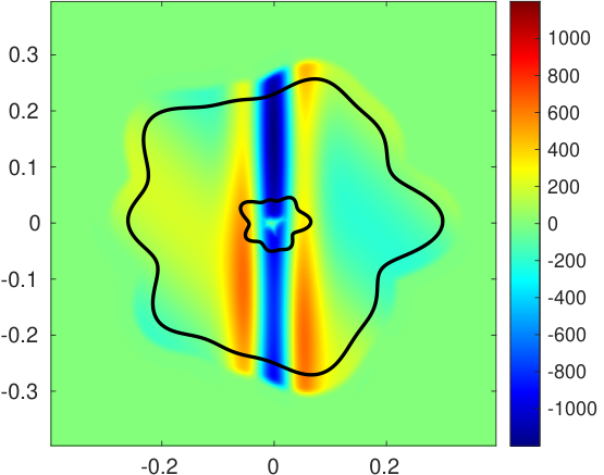
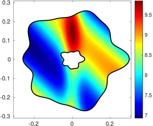
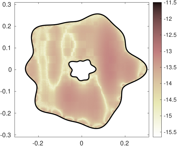
We set the spacing $h$ of the uniform grid to $25$ logarithmically equally spaced points between $10^{-1.4}$ and $10^{-3.5}$ . The number of points $N$ along each dimension varies from $112$ to $1994$ , correspondingly. The convergence order and timing results are shown in fig. 9. We observe that the convergence order is about $6.8$ , and that the timing results exhibit similar pattern as Example 1. The solution to the Dirichlet Poisson problem and its numerical error are shown in fig. 10.

In the third example, the boundary $\Gamma_{3}$ consists of two star fish. The inhomogeneous term in the Poisson equation is

f_{3}(x)=-\sum_{k=0}^{5}e^{-\sqrt{2^{k}}}2^{2k}(\cos(2^{k}x_{1})+\cos(2^{k}x_{2})),\quad x\in\Omega_{3}.

(53)

The boundary data is

g_{3}(x)=\sum_{k=0}^{5}e^{-\sqrt{2^{k}}}(\cos(2^{k}x_{1})+\cos(2^{k}x_{2})),\quad x\in\Omega_{3},

(54)

and the exact solution $u_{3}(x)=g_{3}(x)$ for $x\in\Omega_{3}$ . The boundary $\Gamma_{3}$ , the right-hand side $f_{3}$ , and its 8th order normal extension $f_{3}^{e}$ with $h=10^{-2.2}$ are shown in fig. 11.

(a)

(b)

Figure 12: Left: convergence order study for Example 3. Data points are shown in small circles, while the dashed line is the least squares fitting of first

19

data points, leading to an estimated convergence order

9.6

. Right: timing results for Example 3.

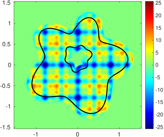
We set the spacing $h$ of the uniform grid to $25$ logarithmically equally spaced points between $10^{-1.1}$ and $10^{-3}$ . The number of points $N$ along each dimension varies from $128$ to $2556$ , correspondingly. The convergence order and timing results are shown in fig. 12. We observe that the convergence order is about $9.6$ , and that the timing results are similar to the first two examples. The solution to the Dirichlet Poisson problem and its numerical error are shown in fig. 13.

Finally, we study the effect of function extension order on the accuracy of the solution. Besides the first three examples, we also consider the case where the boundary is a circle of radius $0.9$ . The exact solution to the Dirichlet Poisson problem is

u_{4}(x)=T_{20}(x_{1})+T_{20}(x_{2}),

(55)

the inhomogeneous term in the Poisson equation $f_{4}(x)=\Delta u_{4}$ , and the Dirichlet data $g_{4}$ is simply the restriction of $u_{4}$ on the boundary. For each example we fix a grid spacing $h,$ and vary the extension order $K$ from $-1$ to $8$ , where $K=-1$ denotes the trivial extension by zero. Figure 14 shows the dependence of accuracy of the solution on the function extension order for all four examples. In all four cases, the accuracy increases as the order of function extension increases.

(a)

(b)

(c)

(d)

Figure 14: The dependence of accuracy of the solution on the function extension order. The

x

-axis is the order of function extension, where

K=-1

denotes the trivial extension by zero. The

y

-axis shows the relative

l^{2}

error of the numerical solution. Top left: the results for Example 1, where the numerical solution is calculated using a

334\times 334

uniform grid with

h\approx 0.0076

. Top right: the results for Example 2, where the numerical solution is calculated using a

406\times 406

uniform grid with

h\approx 0.0019

. Bottom left: the results for Example 3, where the numerical solution is calculated using a

784\times 784

uniform grid with

h\approx 0.0036

. Bottom right: the results for Example 4, where the numerical solution is calculated using a

402\times 402

uniform grid with

h\approx 0.0059

4.3 Three dimensions – FFT-based BVP solvers

We consider two examples in three dimensions to solve the inhomogeneous Dirichlet problem for the Poisson equation using an FFT-based BVP solver. As in the two-dimensional case presented in the previous subsection, function extension is combined with the FFT to generate a particular solution $u^{p}$ . We present timings and convergence plots for the errors with respect to the grid resolution $h$ of the underlying uniform grid. Again, we set the function extension order to $8$ . For the first example we set the parameter $a=1$ in the formulae eq. 29–eq. 30 for computing extension nodes and weights, while in the second example we set $a=0.15$ . The parameters in the window function eq. 42 are set to $c=40.590000152587891$ for $16$ digits of accuracy, and $r_{0}=10^{-6}$ , $r_{1}=32h$ . The error is measured at the subset of $10000$ random points that are inside the given domain, $\Omega$ . These random points are drawn from a uniform distribution over a box with sides such that it just contains $\Omega$ . For the first example the box is $[-0.25,0.25]^{3}$ , and for the second example the box is $[-0.19,0.19]\times[-0.18,0.18]\times[-0.062,0,62]$ .

In the first example the inhomogeneous term in the Poisson equation is given by

f_{4}(x)=-\sin(8\pi x_{1})\sin(8\pi x_{2})\sin(8\pi x_{3}),\quad x\in\Omega_{4},

(56)

with boundary data

g_{4}(x)=\sin(8\pi x_{1})\sin(8\pi x_{2})\sin(8\pi x_{3})/(1536\pi^{3}),\quad x\in\Gamma_{4}.

(57)

Here, $\Omega_{4}$ is the ball with radius $0.25$ . The exact solution $u_{4}(x)$ is given by $g_{4}(x)$ for $x\in\Omega_{4}$ .

The grid spacing $h$ of the uniform grid ranges over $23$ logarithmically equally distributed points between $10^{-2}$ and $10^{-2.75}$ , corresponding to $N=120$ and $N=358$ , respectively. In fig. 15 we observe the expected $10$ th order convergence in the error as a function of the grid resolution $h$ . The error saturates $10^{-9}$ for values of $h$ less than $10^{-2.6}$ , which is probably due to package used for solving the homogeneous Laplace equation [13]. An extension $f^{e}_{4}$ and the Dirichlet data are shown in fig. 16.

In fig. 15 timings are presented. For the three-dimensional setting there are two dominant steps: solving the Laplace equation and sorting points in the uniform grid. As is clear from the plots, function extension and the FFT require relatively little work.

(a)

(b)

Figure 15: Left: convergence order study for Example 4. Data points are shown in small circles, while the dashed line is a reference line corresponding to

\mathcal{O}(h^{10})

. Right: timing results for Example 4, where the x-axis is the number of points along each dimension. Thus, the total number of equispaced grid points in the volume is

N^{3}

For the second example we consider a stellarator-like geometry, given by a surface $\Gamma_{5}$ parameterized by $\mathbf{X}:[0,2\pi]^{2}\rightarrow\Gamma_{5}$ with

\mathbf{X}(u,v)=\sum\limits_{i=-1}^{2}\sum\limits_{j=-1}^{1}\delta_{i,j}\begin{bmatrix}\cos(v)\cos((1-i)u+jv)\\ \sin(v)\cos((1-i)u+jv)\\ \sin((1-i)u+jv)\end{bmatrix}.

(58)

The non-zero coefficients are $\delta_{-1,-1}=0.17$ , $\delta_{-1,0}=0.11$ , $\delta_{0,0}=1$ , $\delta_{1,0}=4.5$ , $\delta_{2,0}=-0.25$ , $\delta_{0.1}=0.07$ , and $\delta_{2,1}=-0.45$ . We let $\Omega_{5}$ denote the solid torus bounded by $\Gamma_{5},$ see fig. 18.

We use the following inhomogeneous term for the Poisson equation,

\displaystyle\begin{split}f_{5}(x)&=-300\sin(10(x_{1}+x_{2}+x_{3}))+2+6x_{3}\\ &+1000e^{-500x^{2}}(500x_{1}^{2}-1)+1000e^{-500x_{3}^{2}}(500x_{3}^{2}-1),\quad x\in\Omega_{5},\end{split}

(59)

with boundary data

g_{5}(x)=\sin(10(x_{1}+x_{2}+x_{3}))+x_{1}^{2}-3x_{2}+x_{3}^{3}+e^{-500x_{1}^{2}}+e^{-500x_{3}^{2}},\quad x\in\Gamma_{5}.

(60)

Again, the exact solution $u_{5}(x)$ is given by $g_{5}(x)$ for $x\in\Omega_{5}$ . The plots in fig. 18 show the stellarator-like geometry, an extension $f_{5}^{e}$ and the Dirichlet boundary data $g_{5}$ .

For this example, the grid spacing $h$ of the uniform grid ranges over $22$ logarithmically equally distributed points between $10^{-2.2}$ to $10^{-2.9}$ , which corresponds to $N=126$ and $N=364$ , respectively. The error as a function of $h$ is shown in fig. 17. As for the previous example, we observe the expected 10th order convergence; the error is saturated for values of $h$ less than $10^{-2.62}$ . As remarked above, this saturation is probably due to limitations in the solver for the homogeneous Laplace equation.

Due to the presence of very narrow regions in $\Omega_{5}$ , we have to set $a=0.15$ , or smaller, to ensure that the points $y-t_{j}x\nu_{y}$ (see formula eq. 6) for each boundary point $y$ all lie inside $\Omega_{5}$ . Note that $a=0.15$ gives $\|w\|_{1}\sim\mathcal{O}(10^{11})$ , however it is clear from the convergence plot in fig. 17 that we nonetheless get the same accuracy as in the previous example, which uses the sphere with $a=1$ .

Concerning the timings, we observe the same trends as for the previous example in three dimensions: solving the Laplace equation and sorting the points are the two most time consuming tasks.

(a)

(b)

Figure 17: Left: convergence order study for Example 5. Data points are shown in small circles, while the dashed line is a reference line corresponding to

\mathcal{O}(h^{10})

. Right: timing results for Example 5.

5 Conclusions and further discussions

We have constructed a function extension scheme along normal directions. The extension formula is given by a linear combination of function values in the specified domain, with explicit expressions for nodes and weights that can be pre-computed. The nodes are Chebyshev nodes scaled by the distance from the extension point to the boundary in the normal direction. Each point in the $p$ th order extension necessitates the evaluation of the $p+1$ function values in the original domain. Moreover, the smoothness order of the extended part along tangential directions remains consistent with the original function. We have incorporated this new function extension scheme into an FFT-based elliptic BVP solver on a uniform grid. The resulting scheme is both accurate and efficient.

This scheme can also be integrated with adaptive volume grids, such as the box FMM (fast multipole method). Consequently, the modified scheme can tackle elliptic BVPs with highly nonuniform data in complex geometries. In practical applications, we have observed that the function extension scheme remains robust; the extended function retains high accuracy even when the extension direction slightly deviates from the normal direction. It is feasible to extend this new scheme along coordinate lines, potentially resulting in more efficient function extension schemes when the function in the original domain is provided, for instance, via polynomial interpolation on each element. These issues are currently under investigation.

Acknowledgments

The authors would like to thank Travis Askham at New Jersey Institute of Technology for helpful discussions. The second author gratefully acknowledges the support from the Knut and Alice Wallenberg Foundation under grant 2020.0258.

References

[1] T. G. Anderson, H. Zhu, and S. Veerapaneni, A fast, high-order scheme for evaluating volume potentials on complex 2d geometries via area-to-line integral conversion and domain mappings, Journal of Computational Physics, 472 (2023), p. 111688.
[2] T. Askham, Integral-equation methods for inhomogeneous elliptic partial differential equations in complex geometry, PhD thesis, New York University, 2016.
[3] T. Askham, A. Barnett, D. Malhotra, J. Hoskins, L. Lu, L. Greengard, M. O’Neil, M. Rachh, and F. Vico et al., FMM3D software library. https://github.com/flatironinstitute/FMM3D, 2023.
[4] T. Askham, Z. Gimbutas, L. Greengard, L. Lu, M. O’Neil, M. Rachh, and V. Rokhlin, fmm2d software library. https://github.com/flatironinstitute/fmm2d, 2021.
[5] T. Askham, J. Hoskins, L. Lu, M. O’Neil, M. Rachh, and F. Vico et al., fmm3dbie software library. https://github.com/fastalgorithms/fmm3dbie, 2023.
[6] A. H. Barnett et al., Non-uniform fast Fourier transform library of types $1$ , $2$ , $3$ in dimensions $1$ , $2$ , $3$ . https://github.com/ahbarnett/finufft, 2018.
[7] R. Bott and L. Tu, Differential forms in algebraic topology, vol. 82 of GTM, Springer-Verlag, 1982.
[8] O. P. Bruno and J. Paul, Two-dimensional Fourier continuation and applications, SIAM Journal on Scientific Computing, 44 (2022), pp. A964–A992.
[9] L. Demanet and A. Townsend, Stable extrapolation of analytic functions, Foundations of Computational Mathematics, 19 (2019), pp. 297–331.
[10] F. Fryklund and L. Greengard, An fmm accelerated poisson solver for complicated geometries in the plane using function extension, 2022.
[11] F. Fryklund, E. Lehto, and A.-K. Tornberg, Partition of unity extension of functions on complex domains, Journal of Computational Physics, 375 (2018), pp. 57–79.
[12] W. Gautschi and G. Inglese, Lower bounds for the condition number of Vandermonde matrices, Numerische Mathematik, 52 (1987), pp. 241–250.
[13] L. Greengard, M. O’Neil, M. Rachh, and F. Vico, Fast multipole methods for the evaluation of layer potentials with locally-corrected quadratures, Journal of Computational Physics: X, 10 (2021), p. 100092.
[14] J. Helsing and A. Karlsson, On a helmholtz transmission problem in planar domains with corners, Journal of Computational Physics, 371 (2018), pp. 315–332.
[15] D. Huybrechs, On the Fourier extension of nonperiodic functions, SIAM Journal on Numerical Analysis, 47 (2010), pp. 4326–4355.
[16] M. B. Kennel, Kdtree 2: Fortran 95 and c++ software to efficiently search for near neighbors in a multi-dimensional euclidean space, 2004.
[17] R. Kress, Linear Integral Equations, vol. 82 of Applied Mathematical Sciences, Springer–Verlag, Berlin, third ed., 2014.
[18] T. Rivlin, An Introduction to Approximation Theory, Dover Press, New York, 1969.
[19] R. T. Seeley, Extension of ${C}^{\infty}$ functions defined in a half space, Proceedings of the American Mathematical Society, 15 (1964), pp. 625–626.
[20] D. Shirokoff and J. Nave, A sharp-interface active penalty method for the incompressible Navier–Stokes equations, J. Sci. Comput., 62 (2015), pp. 53–77.
[21] D. Slepian and H. O. Pollak, Prolate spheroidal wave functions, Fourier analysis and uncertainty — I, The Bell System Technical Journal, 40 (1961), pp. 43–63.
[22] D. B. Stein, Spectrally accurate solutions to inhomogeneous elliptic pde in smooth geometries using function intension, Journal of Computational Physics, 470 (2022), p. 111594.
[23] D. B. Stein, R. D. Guy, and B. Thomases, Immersed boundary smooth extension (ibse): A high-order method for solving incompressible flows in arbitrary smooth domains, Journal of Computational Physics, 335 (2017), pp. 155–178.
[24] M. Webb, L. N. Trefethen, and P. Gonnet, Stability of barycentric interpolation formulas for extrapolation, SIAM Journal on Scientific Computing, 34 (2012), pp. A3009–A3015.
[25] H. Zhu and S. Veerapaneni, High-order close evaluation of laplace layer potentials: A differential geometric approach, SIAM Journal on Scientific Computing, 44 (2022), pp. A1381–A1404.

August 11, 2026