Route to Time and Time to Route:
Travel Time Estimation from Sparse Trajectories

Let $X$ be the features of the road (e.g., road types, road lanes) and $Z$ be the unobserved true travel-time distribution of $K$ road segments that we want to predict. The goal is to learn a discriminative model $f$ that predicts the true target $Z$ from the feature vector $X$, so as to maximize the conditional probability $P(Z\mid X)$. Here, the travel time distribution $Z$ highly depends on the real-time traffic condition. Intuitively, we discretize one day into $\mathcal{I}$ time steps (i.e., a specific time window $\Delta t$=30 minutes). So given a trajectory $Tr$ at time step $t_{s}$, which can be denoted as sequence of sampled GPS point: $p_{1}\rightarrow p_{2}\rightarrow\cdots\rightarrow p_{|Tr|}$, $\widetilde{r}$ is the most likely route (bag) between two continuous GPS points $p_{a}$ and $p_{b}$ during $Tr$, where $|\widetilde{r}|=K$ denotes the number of total travelled road segments in $\widetilde{r}$. Especially, $X_{1:K}$¹¹ 1 The subscript for example $X_{1:K}$ denotes an abbreviation for the set $\{X_{1},X_{2},\cdots,X_{K}\}$ stands for the bag of the travelled road segments’ features corresponding to $\widetilde{r}$. $W$ is the collection of all weight parameters in the neural network $f$ to learn $Z$. $T_{a,b}$ is the actual observation of total time cost between $p_{a}$ and $p_{b}$.

Fig. 2 illustrates the data generation process with a graphical representation. Given $p_{a}$ and $p_{b}$, we first infer the most likely route $\widetilde{r}$ from the road network with $P(\widetilde{r}\mid p_{a},p_{b},Z)$, which is equal to estimate $P(X_{1:K}\mid p_{a},p_{b},Z_{1:K})$. Subsequently, we generate the conditional probability $P\left(Z_{i}\mid\theta\right)$ for each travel time distribution $Z_{i}$. Specifically, we here assume that each latent variable $Z_{i}$ belongs to the Lognormal distribution $Z_{i}\sim\frac{1}{z\sigma\sqrt{2\pi}}\exp\left(-\frac{(\ln z-\mu)^{2}}{2\sigma^{2}}\right)$ [17]. We let the conditional probability $P\left(Z_{i}\mid\theta\right)=P\left(Z_{i}\mid\left(\mu,\sigma\right)=f\left(X;W\right)\right)$, where $W$ and $X$ are the cofactors that generate the parameterized $\mu$ and $\sigma$ of $Z_{i}$ by the deterministic function $f$. Consequently, total travel time $T_{a,b}$ can be observed by an aggregate function $Q$ with $T_{a,b}=Q(Z_{1:K})=\sum_{i=1}^{K}Z_{i}$.

Here, we summarize the two basic assumptions used in our paper.
Assumption 1 (Aggregate observation assumption) $P(T_{a,b}\mid X_{1:K},Z_{1:K})=P(T_{a,b}\mid Z_{1:K})$

We assume that observation $T_{a,b}$ is conditionally independent on $X_{1:K}$ when given $Z_{1:K}$. This assumption is informed by existing studies [2] and conforms to the TTE problem, since given $Z_{1:K}$, observation $T_{a,b}$ can be determined by aggregate function $Q$.

We assume that $Z_{i+1}$ are mutually independent except for $Z_{i}$. This is under the assumption of a Markov chain and is based on extensive applications in trajectory data mining [1]. Furthermore, since $T_{a,b}$ can be determined by the function $Q$, the conditional probability can be defined as $P(T_{a,b}\mid Z_{1:K})=\delta_{Q\left(Z_{1:K}\right)}(T_{a,b})$, where $\delta(\cdot)$ represents the Dirac delta function.

In summary, the objective function in this paper can be written as follows.

which is the maximum of a posterior estimation by taking the $Z$ as latent variables with the observation of sparse travel time $T_{a,b}$. Therefore, we divide the training process into expectation ($E$ step) and maximization ($M$ step) according to the above assumptions.

E step aims to estimate the travel time of the most likely route $\widetilde{r}$ by learned travel time distribution $Z$ through weakly supervised learning, and M step heuristically searches $\widetilde{r}$ from the candidate set $\Omega_{a,b}=\{r_{1},r_{2},\cdots,r_{m}\}$ to reduce the computational cost. According to the above EM procedure, we obtain the estimated route $\widetilde{r}$ for every pair of $p_{a}$ and $p_{b}$, as well as travel time distribution $Z$. Thus, the final travel time of trajectory $Tr$ can be obtained by summing all the estimation components $\Theta=\{\widetilde{T}_{1},\widetilde{T}_{2},\cdots,\widetilde{T}_{|Tr|-1}\}$ between every continuous GPS sample with $\widetilde{T}=\sum_{i=1}^{|Tr|-1}\widetilde{T}_{i}$, where $\widetilde{T}_{i}$, produced by $f$, denotes the forecast travel time of $p_{i}$ and $p_{i-1}$.

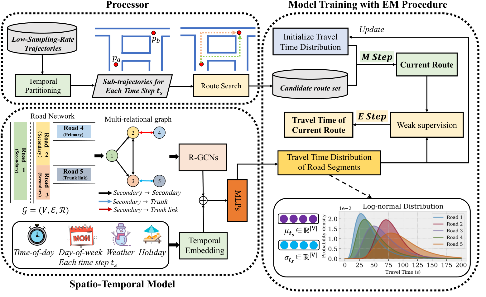
Fig. 3 shows our proposed WSL-TTE system with the EM algorithm, which consists of three main components - processor, spatio-temporal model and model training with EM procedure.

$(1)$ Processor temporally partitions the low-sampling-rate historical trajectories from the datasets into each time step $t_{s}$.

$(2)$ Spatio-Temporal Model $f$ estimates the travel time distribution $Z$ of the road segments. We firstly transform a road network into a multi-relational graph $\mathcal{G}$, and encode each time step $t_{s}$ into a vector. Then we fuse the aforementioned spatial representation and temporal encoding as the time-variant vertex representations. In the final, $\mu_{t_{s}}$ and $\sigma_{t_{s}}$ of travel time distribution $Z$ are parameterized by two MLPs (Multi-Layer Perception).

(3) Model Training with EM Procedure is used to optimize the learned $Z$ in $E$-step using Eq. (3.6) and infer route $\widetilde{r}$ by Eq. (6). Travel time distribution $Z$ is initially default as $\mu=\frac{L_{i}}{\mathbf{S}_{i}}$ and $\sigma=1$, where $L_{i}$ and $\mathbf{S}_{i}$ are the length and speed limits of $i^{th}$ road segment, respectively. The EM algorithm will be finished when the estimated variables $Z$ converge.

The spatio-temporal model aims to learn $f$ to estimate travel time distribution $Z$ of road segments from road network. Fig. 4(a) shows the locations of the neighbors of Yongquan Street, and Fig. 4(b) depicts the maximum, minimum and average traffic speed during Chinese national day. We observe several phenomena: 1) road speed is highly related to the road types; and 2) the road speed is also affected by the type of connection road. For example, Yongquan road and Liyuan street are residential and secondary roads, respectively. Even though they are neighbors, the road speeds are relatively different. Thus, the road network is represented as a multi-relational graph $\mathcal{G}=(\mathcal{V},\mathcal{E},\mathcal{R})$, where $\mathcal{V}$ denotes the set of vertices (i.e. road segments) and $\mathcal{E}$ denotes the set of edges. An edge $\mathbf{e}_{ijk}=(v_{i},v_{j},\mathbf{r}_{k})\in\mathcal{E}$ indicates that the road segment $v_{i}\in\mathcal{V}$ connects to the road segment $v_{j}\in\mathcal{V}$ with a relation type $\mathbf{r}_{k}\in\mathcal{R}$.

Based on this multi-relational graph, we adopt a 3-layer Relational Graph Convolution Networks (R-GCNs) [19] as the building block to learn the graph structure information. $l^{th}$ R-GCN can be defined as

where $h_{v_{i}}^{(l)}\in\mathbb{R}^{d^{(l)}}$ is the hidden state of road segment $v_{i}$ in the $l^{th}$ layer of the model with dimension $d^{(l)}$ and $W_{\mathbf{r}_{k}}^{(l)},W_{0}^{(l)}$ present the learnable parameters. $\mathcal{N}_{i}^{\mathbf{r}_{k}}$ denotes the set of neighbor indices of node $v_{i}$ in relation to $\mathbf{r}_{k}\in\mathcal{R}$. $c_{i,\mathbf{r}_{k}}$ is the normalization constant. Note that $h_{v_{i}}^{(0)}$ is the spatial feature $X_{v_{i}}$ of road segment $v_{i}$. We use the embedding layer to encode the following statistical features:

• $\bullet$

  Road types: for example, primary, primary link, secondary, secondary link;

• $\bullet$

  Number of lanes: how many marked traffic lanes;

• $\bullet$

  Whether it is one way or not.

The final output of R-GCNs, represented as $s_{v_{i}}\in\mathbb{R}^{D}$, where $v_{i}\in\mathcal{V}$. But spatial representation $s_{v_{i}}$ only provides the static representation, which could not show the temporally dynamic correlations for each road segment.

As we mentioned previously, the spatio-temporal model $f$ is to estimate the mean value $\mu$ and variance $\sigma$ of Lognormal distribution for each road segment $v_{i}$ at each time step $t_{s}$. Intuitively, we encode the day-of-week and time-of-day of each time step $t_{s}$ into $\mathbb{R}^{7}$ and $\mathbb{R}^{\mathcal{I}}$ using one hot encoding, and concatenate them with the embedding of weather conditions and HolidayID (holiday or not). Then we use one-layer MLP to transform the above temporal embedding vector into a vector $s_{t_{s}}\in\mathbb{R}^{D}$, which is equal to the spatial representation $s_{v_{i}}$. To obtain the time-variant road segment representations, we fuse the above spatial representation and reconstruct temporal embedding vector: for each road segment $s_{v_{i}}$ at time step $t_{s}$, the spatio-temporal representation is defined as $F_{v_{i},t_{s}}=s_{v_{i}}+s_{t_{s}}$, which contains both spatial road structure and temporal information.

Based on the spatio-temporal representation $F\in\mathbb{R}^{(|\mathcal{V}|*N_{t_{s}})\times D}$, where $N_{t_{s}}$ denotes the total number of time steps, $\mu_{t_{s}}\in\mathbb{R}^{|\mathcal{V}|}$ and $\sigma_{t_{s}}\in\mathbb{R}^{|\mathcal{V}|}$ for each time step $t_{s}\in\mathbb{R}^{N_{t_{s}}}$ are parameterized by two-layer MLPs with shared fused representation $F$.

Next, we introduce the learning procedure of estimated travel time distribution $Z$ through weakly supervised learning. The aforementioned expected log-likelihood in Equation (2) defines the aggregate expectation from $Z$ to $T$. Here, we assume the distribution $T_{a,b}$ also under the Lognormal distribution approximated by summation of all $Z_{1:K}$ on route $r$ [5] as

Thus, the term of expectation in Eq. (2) can be derived to be

Here, we introduce how to maximize the conditional probability in Eq. (3). Given two continuous samples $p_{a}$, $p_{b}$, and the last-step parameters $W^{(i)}$ produced from Eq. (3.6), our objective is to find the optimal route $\widetilde{r}$ with the travel time closest to the observation $T_{a,b}$. As mentioned in [8], it is natural to assume that the route $\widetilde{r}$ is very likely to be among the top $m$-shortest paths between $p_{a}$ and $p_{b}$. Therefore, we utilize Yen’s algorithm [27] to generate the candidate set $\Omega_{a,b}=\{r_{1},r_{2},\cdots,r_{m}\}$ and the optimal route $\widetilde{r}$ can be selected by

We perform Eq. (6) for every pair of continuous samples to update their corresponding route $\widetilde{r}$. Furthermore, to prevent extensive overlap in $\Omega_{a,b}$, this paper leverages the weighted Jaccard ($wJCD$) value to calculate each pair of routes $r_{i},r_{j}\in\Omega_{a,b}$ referring to [8]. The EM algorithm will complete when it reaches the estimated variables $\mu$ and $\sigma$ convergence.

• $\bullet$

  DeepTTE: [23] is an end-to-end deep learning framework, which infers the travel time from both the entire path and each local path simultaneously.

• $\bullet$

  DeepGTT: [11] learns the travel time distribution through the deep generative model, which takes the real-time traffic condition into account.

• $\bullet$

  MVSTM: [14] is a multi-view spatial-temporal model that captures the mutual dependence of spatial-temporal relations and trajectory features.

• $\bullet$

  MURAT: [12] is a multi-task representation learning method by utilizing the underlying road network and the spatio-temporal prior knowledge.

• $\bullet$

  DCRNN: [13] exploits GCN to capture spatial dependency and then uses recurrent neural networks to model temporal dependency.

• $\bullet$

  ConSTGAT: [6] adopts a graph attention mechanism to explore the joint relations of spatio-temporal information.

• $\bullet$

  T-GCN: [31] proposes a temporal GCN model that combines the GCN and GRU to simultaneously extract the spatial and temporal dependencies.

Additionally, three state-of-the-art algorithms STRS [25], MTrajRec [18], and DeepGTT [11] are used as baseline models for route recovery. STRS and DeepGTT learn the travel time of the road network and conduct the route search for low-sampling-rate trajectories. MtrajRec recoveries the route via a two-stage Seq2Seq model based on coarse grid representation.

We conducted a real-world case study in Chengdu, which visualizes the learned road conditions using our proposed WSL-TTE. To acquire the road conditions of the road network, we here transform travel time $\mu$ estimated by our WSL-TTE into the average speed by $Speed_{i}=\frac{Length_{i}}{\mu_{i}}$ for each road $v_{i}$. Four kinds of colors are used to represent the different road states, which can be defined as 1) red - very congested, 2) yellow - congested, 3) orange - slow, and 4) green - unblocked. We equally divide the limiting velocity for each road type and set the speed interval for these four road states. For example, the speed limit of the primary road type is $60kph$, then the speed range that represents very congested is $[0,15)$, congested is $[15,30)$, slow is $[30,45)$ and unblocked is $[45,60)$. We calculate the average speeds by the original dense trajectories as the ground truth. Specifically, we mark them with an unblocked state for the roads without a trajectory. The compared result is shown in Fig. 6, our model can generate approximate road conditions with ground truth for both non-rush and rush hour.

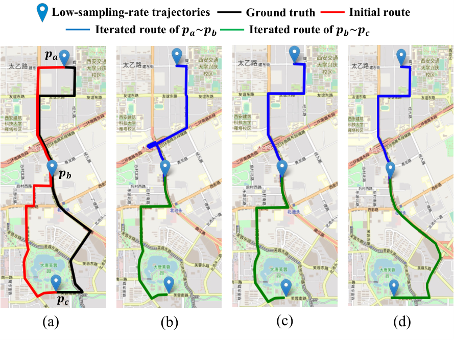
In addition, we provide a visualization example of the route update process in route recovery. As is shown in Fig. 7, our route update process with the EM algorithm can gradually find the approximate route with ground truth, owing to the precise travel time, which demonstrated our previous assumption that: the more precise travel time can lead to a better inference of routes, in turn, resulting in more accurate time estimation.

The parameter settings used in our experiment are described as follows:

• $\bullet$

  In the generation of a candidate route set $\Omega_{a,b}$, $m$ candidate routes are selected between the two given low sample rate GPS points. Here, $m=5$ is used for both Xi’an and Porto, and $m=7$ for Chengdu, respectively. All three hyper-parameters can ensure that over 90 percents of ground truth route can be acquired from $\Omega_{a,b}$.

• $\bullet$

  In the spatial R-GCN layers, the embedding sizes of road feature representation (road types, number of lanes and one way or not) are set to 8, 4, 2 respectively.

• $\bullet$

  In the temporal embedding component, we embed WeatherID and HolidayID in $R^{8}$ and $R^{4}$, respectively.

The experiments are implemented with PyTorch 1.6.0 and Python 3.6 and are trained with a RTX2080 GPU. The platform ran on Ubuntu 16.04 OS. Our model is optimized by Adams with an initial learning rate 0.0001 for 20 epochs, and early stopping is used on the test dataset. We select the best hyper-parameter setting for the baseline methods on the valuation dataset.

In addition, to validate the effectiveness of the learned travel time distributions of road segments, we also select two road segments from the Xi’an road network with the similar travel time. One is a busy road segment (type: “primary”), the other is a highway. From Fig. 1, we can find that learned travel time distributions for both two roads have the obvious morning and evening rush hours. Meanwhile, this primary road has a relatively more considerable variance than the highway. This demonstrates that our WSL can acquire reasonable travel time distributions of road network.

References

- [1] Brakatsoulas, S., Pfoser, D., Salas, R., Wenk, C.: On map-matching vehicle tracking data. In: Proceedings of the 31st international conference on Very large data bases. pp. 853–864 (2005)
- [2] Carbonneau, M.A., Cheplygina, V., Granger, E., Gagnon, G.: Multiple instance learning: A survey of problem characteristics and applications. Pattern Recognition 77, 329–353 (2018)
- [3] Chen, Y., Bi, J., Wang, J.Z.: Miles: Multiple-instance learning via embedded instance selection. IEEE Transactions on Pattern Analysis and Machine Intelligence 28(12), 1931–1947 (2006)
- [4] Dempster, A.P., Laird, N.M., Rubin, D.B.: Maximum likelihood from incomplete data via the em algorithm. Journal of the Royal Statistical Society: Series B (Methodological) 39(1), 1–22 (1977)
- [5] Dufresne, D.: Sums of lognormals. In: Actuarial Research Conference. pp. 1–6 (2008)
- [6] Fang, X., Huang, J., Wang, F., Zeng, L., Liang, H., Wang, H.: Constgat: Contextual spatial-temporal graph attention network for travel time estimation at baidu maps. In: Proceedings of the 26th ACM SIGKDD International Conference on Knowledge Discovery & Data Mining. pp. 2697–2705 (2020)
- [7] Frénay, B., Verleysen, M.: Classification in the presence of label noise: a survey. IEEE transactions on neural networks and learning systems 25(5), 845–869 (2013)
- [8] He, T., Bao, J., Li, R., Ruan, S., Li, Y., Song, L., He, H., Zheng, Y.: What is the human mobility in a new city: Transfer mobility knowledge across cities. In: Proceedings of The Web Conference 2020. pp. 1355–1365 (2020)
- [9] Idé, T., Sugiyama, M.: Trajectory regression on road networks. In: Proceedings of the AAAI Conference on Artificial Intelligence. vol. 25 (2011)
- [10] Jabari, S.E., Freris, N.M., Dilip, D.M.: Sparse travel time estimation from streaming data. Transportation Science 54(1), 1–20 (2020)
- [11] Li, X., Cong, G., Sun, A., Cheng, Y.: Learning travel time distributions with deep generative model. In: The World Wide Web Conference. pp. 1017–1027 (2019)
- [12] Li, Y., Fu, K., Wang, Z., Shahabi, C., Ye, J., Liu, Y.: Multi-task representation learning for travel time estimation. In: Proceedings of the 24th ACM SIGKDD International Conference on Knowledge Discovery & Data Mining. pp. 1695–1704 (2018)
- [13] Li, Y., Yu, R., Shahabi, C., Liu, Y.: Diffusion convolutional recurrent neural network: Data-driven traffic forecasting. arXiv preprint arXiv:1707.01926 (2017)
- [14] Liu, Z., Wu, Z., Wang, M., Zhang, R.: Multi-view spatial-temporal model for travel time estimation. In: Proceedings of the 29th International Conference on Advances in Geographic Information Systems. pp. 646–649 (2021)
- [15] Lou, Y., Zhang, C., Zheng, Y., Xie, X., Wang, W., Huang, Y.: Map-matching for low-sampling-rate gps trajectories. In: Proceedings of the 17th ACM SIGSPATIAL international conference on advances in geographic information systems. pp. 352–361 (2009)
- [16] Mil, S., Piantanakulchai, M.: Modified bayesian data fusion model for travel time estimation considering spurious data and traffic conditions. Applied Soft Computing 72, 65–78 (2018)
- [17] Pu, W.: Analytic relationships between travel time reliability measures. Transportation Research Record 2254(1), 122–130 (2011)
- [18] Ren, H., Ruan, S., Li, Y., Bao, J., Meng, C., Li, R., Zheng, Y.: Mtrajrec: Map-constrained trajectory recovery via seq2seq multi-task learning. In: Proceedings of the 27th ACM SIGKDD Conference on Knowledge Discovery & Data Mining. pp. 1410–1419 (2021)
- [19] Schlichtkrull, M., Kipf, T.N., Bloem, P., Van Den Berg, R., Titov, I., Welling, M.: Modeling relational data with graph convolutional networks. In: European semantic web conference. pp. 593–607. Springer (2018)
- [20] Shao, K., Wang, K., Chen, L., Zhou, Z.: Estimation of urban travel time with sparse traffic surveillance data. In: Proceedings of the 2020 4th High Performance Computing and Cluster Technologies Conference & 2020 3rd International Conference on Big Data and Artificial Intelligence. pp. 218–223 (2020)
- [21] Tiesyte, D., Jensen, C.S.: Similarity-based prediction of travel times for vehicles traveling on known routes. In: Proceedings of the 16th ACM SIGSPATIAL international conference on Advances in geographic information systems. pp. 1–10 (2008)
- [22] Veličković, P., Cucurull, G., Casanova, A., Romero, A., Lio, P., Bengio, Y.: Graph attention networks. arXiv preprint arXiv:1710.10903 (2017)
- [23] Wang, D., Zhang, J., Cao, W., Li, J., Zheng, Y.: When will you arrive? estimating travel time based on deep neural networks. In: Thirty-Second AAAI Conference on Artificial Intelligence (2018)
- [24] Wang, Y., Zheng, Y., Xue, Y.: Travel time estimation of a path using sparse trajectories. In: Proceedings of the 20th ACM SIGKDD international conference on Knowledge discovery and data mining. pp. 25–34 (2014)
- [25] Wu, H., Mao, J., Sun, W., Zheng, B., Zhang, H., Chen, Z., Wang, W.: Probabilistic robust route recovery with spatio-temporal dynamics. In: Proceedings of the 22nd ACM SIGKDD International Conference on Knowledge Discovery and Data Mining. pp. 1915–1924 (2016)
- [26] Yang, C., Gidofalvi, G.: Fast map matching, an algorithm integrating hidden markov model with precomputation. International Journal of Geographical Information Science 32(3), 547–570 (2018)
- [27] Yen, J.Y.: Finding the k shortest loopless paths in a network. management Science 17(11), 712–716 (1971)
- [28] Yuan, J., Zheng, Y., Zhang, C., Xie, X., Sun, G.Z.: An interactive-voting based map matching algorithm. In: 2010 Eleventh international conference on mobile data management. pp. 43–52. IEEE (2010)
- [29] Yun, S., Jeong, M., Kim, R., Kang, J., Kim, H.J.: Graph transformer networks. Advances in Neural Information Processing Systems 32, 11983–11993 (2019)
- [30] Zhang, Y., Charoenphakdee, N., Wu, Z., Sugiyama, M.: Learning from aggregate observations. arXiv preprint arXiv:2004.06316 (2020)
- [31] Zhao, L., Song, Y., Zhang, C., Liu, Y., Wang, P., Lin, T., Deng, M., Li, H.: T-gcn: A temporal graph convolutional network for traffic prediction. IEEE Transactions on Intelligent Transportation Systems 21(9), 3848–3858 (2019)
- [32] Zhou, Z.H.: A brief introduction to weakly supervised learning. National science review 5(1), 44–53 (2018)
- [33] Zhou, Z.H., Sun, Y.Y., Li, Y.F.: Multi-instance learning by treating instances as non-iid samples. In: Proceedings of the 26th annual international conference on machine learning. pp. 1249–1256 (2009)
A APPENDIX
A.1 Datasets
Road Networks. The matching road network database has been collected from OpenStreetMap for three regions, including Porto, Xi’an and Chengdu. Here, the Porto road network possesses 10334 edges and 9072 nodes, the Xi’an road network ranges from 34.20°to 34.29°in latitude and 108.90°to 108.99°in longitude, and it contains 4780 edges and 3782 nodes, and the Chengdu road network contains 8221 edges and 5182 nodes. All three road networks included nine road types (trunk, trunk link, freeway link, primary, primary link, secondary, secondary link, tertiary, tertiary link). In this paper, we use the Fast Map Matching (FMM) algorithm [26] to map the vehicle trajectory onto the road network.
Taxi Trajectories. We use three real-world taxi datasets to evaluate our proposed method. Porto22 2 https://www.kaggle.com/c/pkdd-15-predict-taxi-service-trajectory-i/data dataset contains the taxi trajectories of 442 taxis in May 2014. Xi’an and Chengdu come from Didi Chuxing Open Data, which are October 2016 and August 2014 respectively. The GPS points of both two datasets have been tied to the road and the interval of sample trajectory points is 2-4s. Especially, we further collected the corresponding weather conditions 33 3 https://www.timeanddate.com/weather ( 6 types including temperature, wind, visibility, etc.) of each trajectory for all three datasets.
A.2 Hyper-parameter Setting