RendNet: Unified 2D/3D Recognizer with Latent Space Rendering
Abstract
Vector graphics (VG) have been ubiquitous in our daily life with vast applications in engineering, architecture, designs, etc. The VG recognition process of most existing methods is to first render the VG into raster graphics (RG) and then conduct recognition based on RG formats. However, this procedure discards the structure of geometries and loses the high resolution of VG. Recently, another category of algorithms is proposed to recognize directly from the original VG format. But it is affected by the topological errors that can be filtered out by RG rendering. Instead of looking at one format, it is a good solution to utilize the formats of VG and RG together to avoid these shortcomings. Besides, we argue that the VG-to-RG rendering process is essential to effectively combine VG and RG information. By specifying the rules on how to transfer VG primitives to RG pixels, the rendering process depicts the interaction and correlation between VG and RG. As a result, we propose RendNet, a unified architecture for recognition on both 2D and 3D scenarios, which considers both VG/RG representations and exploits their interaction by incorporating the VG-to-RG rasterization process. Experiments show that RendNet can achieve state-of-the-art performance on 2D and 3D object recognition tasks on various VG datasets.
1 Introduction

Deep learning has opened a new era for visual perception with machines. Most current methods deal with sensory input such as pixel images, called raster graphics (RG). They benefit from the easy accessibility of input data. However, for human drafted graphics like floor plans, graphic designs, and CAD models, another data format is widely used, called vector graphics (VG). In this paper, we focus on recognition tasks taking VG as input, such as VG-based image classification and object detection.
Vector graphics contain a set of primitives defined with parametric equations, such as lines, curves, and circles, which are almost impossible for a human to directly perceive. It needs to be rendered into the format as the raster graphics by rasterization technique (as shown in Fig. 1), so it can be displayed on monitors or printed on paper. Most of the existing VG recognizers take the rendered RG as input, taking advantage of mature RG-based recognition methods like convolutional neural networks he2016deep or PointNet qi2017pointnet. However, rendered pixels discard the structure of geometries and lose the high-resolution property of VG. As a result, recently some pioneering works jiang2021recognizing; uvnet are proposed to directly recognize VG from its original format. Although achieving encouraging performance improvements, VG-based methods are affected by human un-perceivable topological errors, which can be filtered out by rasterization. For example, Fig. 2 shows two lines whose ends shall meet but do not meet by a small margin, and this error is absent in the rendered RG. Different from the existing methods that consider only one format, this paper proposes a method that leverages the merits of both VG and RG.
How to effectively combine the information of VG and RG remains an open question. An intuitive way is to use the separate model on VG and RG respectively and fuse the results. However, it fails to exploit the interactions and correlations between the VG primitives and RG pixels, which is essential to multi-modality feature fusion baltruvsaitis2018multimodal; wang2020incorporating; zadeh2017tensor. As shown in Fig. 1, the VG-to-RG renderer reveals VG/RG correlation by specifying the rules on how to transfer VG primitives to RG pixels. As a result, we consider incorporating the rendering process as a part of our method to better model the interactions and correlations between RG and VG.

In view of these problems, we propose a novel vector graphics recognition method, named RendNet. RendNet leverages both VG/RG representations and exploits their interactions by incorporating the rendering process. It is a unified framework applicable to both 2D and 3D scenarios. Specifically, RendNet takes the VG primitives as input and represents the VG as a hypergraph. The hypergraph is fed into a network with two parallel streams. A ‘vector’ stream handles hypergraph topology and extracts VG embeddings by hypergraph neural networks. A ‘raster’ stream transfers the VG into 2D pixels or 3D point clouds as RG information. To unify the framework, we utilize PointNet as a simple but effective backbone to extract spatial embeddings of RG. Finally, as the core of RendNet, the correlation between VG and RG embeddings is modeled by a novel latent space rasterization (LSR) method, which simulates a rendering process and projects the VG representations to RG latent features. In this way, the VG/RG correlations are exploited at multiple semantic levels throughout the entire network.
Our main contributions: 1) RendNet is a 2D/3D unified vector graphics recognition framework that leverages the merits of both vector graphics and raster graphics. 2) RendNet incorporates the rendering process and effectively exploits the interaction between RG and VG. 3) Experiments are conducted on both classification and object detection tasks on both 2D and 3D datasets. State-of-the-art performances are achieved.
2 Related work
2D VG recognition and generation. Most of the concurrent recognition methods focus on pixel-based raster graphics, such as ResNethe2016deep, R-CNNgirshick2014rich; girshick2015fast; ren2015faster, YOLO redmon2016you; redmon2017yolo9000. Thus, the intuitive way to conduct VG recognition is a two-stage process that applies CNN-based models on rendered VGs. One of the applications of VG recognition is architecture drawing recognition. Several rule-based graph matching methods are proposed to classify and localize symbols by representing symbols in a floor-plan as graphs for matching, such as visibility graph locteau2007symbol and attributed relational graph ramel2000structural; santosh2012symbol. Online handwriting ha2017neural; NEURIPS2020_723e8f97 is a data form similar to vector graphics. Most of these methods use sequential models to handle the point sequence in hand-writing. Compare to online handwriting, VG contains more types of primitives and has a more general and complex topological structure. Another AI application on VG is computer-aided design. In recent years, a few works propose to use deep learning to automatically generate design graphics or convert raster graphics to vector graphics (i.e. vectorization) DBLP:conf/nips/CarlierDAT20; ganin2021computer; reddy2021im2vec; lopes2019learned; shen2021clipgen; parakkat2021color.
3D representations. 3D objects can be represented with different formats including point clouds, voxels, meshes, multi-view images, boundary representations (BRep). Many deep learning techniques have been studied to address various problems on point clouds, such as shape classification, object detection and segmentation 3dsurvey. PointNet qi2017pointnet and PointNet++ qi2017pointnet++ are two pioneering works which capture fine-grained geometric information of each point. PointConv wu2019pointconv defines convolutional kernels and takes a local subset of points as inputs to learn the hierarchical relations. DGCNN wang2019dynamic constructs a graph where the vertex is each point in a point cloud and the edge is generated based on the neighbors of each point. Further, volume-based methods maturana2015voxnet; zhou2018voxelnet usually quantize point clouds or other 3D formats into voxels and utilize 3D convolutional neural networks to learn representations upon. Besides, multi-view methods su2015multi; wei2020view project a 3D shape into multiple 2D views, extract view-wise features, and aggregate into a global representation.
Different from the previous four formats, the boundary representation (BRep), widely used during the CAD modeling process, is made of a variety of parametric primitives such as Bézier curves and planes. It is a typical ‘VG’ data in 3D. Very recently, UV-net and BRepNet uvnet; brepnet are proposed to directly utilize BRep topological information by constructing a graph based on face-edge relations. In contrast to these works, we leverage the merits of two formats, BReps and point clouds by rasterization technique.
Differentiable rendering. Differentiable rendering involves a rendering process where gradients of object attributes can be propagated through the rendering results kato2020differentiable. Recent works pavlakos2018learning; genova2018unsupervised; bao2019high; rhodin2015versatile utilize differentiable rendering to form an unsupervised workflow for human pose detection and face reconstruction, based on consistency between the original image and the rendered image from detected features. In this work, we choose to render the VG primitives in the latent space rather than the pixel space. The rendering target is a point cloud with latent feature attributes, instead of color attributes in normal rendering.
3 Design of RendNet
3.1 Overview
In this section, we describe the framework of our proposed RendNet and then introduce each module in detail. As shown in Fig. 3, it is composed of basic blocks with residual connections and a final block for global representation aggregation.
The original input is a set of primitives. We first convert them into a hypergraph with the initial node features based on Sec. 3.2. Then we learn the hypergraph representation by residual blocks. Inside each block, node embeddings pass through two streams, the vector stream and the raster stream, to perform the graph convolution and point representation aggregation to obtain the new node embeddings . Fig. 4 shows the detailed process of two streams: the vector stream includes vector encoder (Sec. 3.3), which utilizes hypergraph neural networks (hypergraph NN) to aggregate node embeddings mainly based on the connectivity (i.e., nodes connected by curve segment or falling on the same surface); the raster stream involves latent space rasterization (Sec. 3.4) and raster encoder (Sec. 3.5), which renders VG node embeddings as 2D pixels or 3D point clouds and learn the representation in the Euclidean space. We integrate the information from two streams with residual connection to get the new embeddings (Sec. 3.6).
Especially, we highlight the LSR operation because it is the bridge between VG and RG. Through LSR and residual connection among blocks, the information can be propagated in various paths, such as VGLSRRG, LSRRGVG, VGLSRRGVG, etc. Finally, the global aggregation block (Sec. 3.7) learns the final representation for the whole hypergraph, i.e., all the primitives.
3.2 Building the hypergraph
In RendNet, we convert all the primitive descriptions in the vector graphics into a hypergraph to learn latent features. The hypergraph is mainly formed by connectivity and entails the property of each primitive and the topology among primitives at the same time.
Selection of nodes. The intersection of curves, as well as the start and end of curves, are picked as nodes. In addition, if the curve is not a straight line, at least 4 nodes are ensured to be selected on it with farthest point sampling. The node features are coordinates of these points in Euclidean space.
Curves as edges. The curve connectivity of the nodes above naturally forms edges between the nodes. Each curve is broken into segments by nodes, and each segment is formulated as an edge. The edge features include the start direction vector, the end direction vector, and the type of the curve. The feature is selected due to the universality between different types of curves. Also, in most current specifications of vector graphics (such as SVG), all types of curves as lines, arcs, and second-order bezier curve segments, can be uniquely reconstructed from these attributes, up to translational and scaling invariances.
Surfaces as hyperedges. Surfaces connect multiple nodes, and thus they form hyperedges on the hypergraph. The hyperedge features include the type of the surface and the set of parameters of nodes lying on the surface. This encodes the relative positioning of nodes on the surface, which is useful for feature aggregation.
3.3 Vector encoder
The vector encoder aggregates the node/edge/hyperedge features and the hypergraph structure. To achieve it, we utilize hypergraph neural networks to learn node embeddings.
For curve edges, we use the NNConv scheme proposed by Gilmer et al. gilmer2017neural:
| (1) |
where is the set of neighbors of node . We apply as an MLP to map edge features to a coefficient matrix, and then multiply the embeddings of neighbors from the previous -th block. We average the information from neighbors and obtain the curve message .
For surface hyperedges, we adopt the hypergraph message passing design from Feng et al. feng2019hypergraph. The hypergraph message passing consists of two stages, aggregation of connected node embeddings of hyperedges into hyperedge representations, and aggregation of hyperedge representations back to nodes. We improve the message passing scheme with geometry taken into account.
In the first stage, we aggregate the node embeddings in a PointNet qi2017pointnet fashion, i.e. we first concatenate the -th node embeddings with the relative coordinates on the surface in parameter space, then apply the max aggregation to obtain hyperedge-wise representations:
| (2) |
where denotes a surface hyperedge and is the embedding of node that lies on S. We concatenate it with , the type of the surface (rectangle/circle, etc.) and , the coordinates of node on . Through an MLP and a max aggregation, we obtain the representation of . Note that the coordinates for the same node are relative and can be different on different surfaces.
In the second stage, we calculate the hyperedge message for each node by averaging hyperedge representations:
| (3) |
3.4 Latent space rasterization
In RendNet, we employ a tailored rasterization process that follows the general pattern of rasterization in computer graphics (CG) but is specially designed for incorporating in object recognition, namely the Latent Space Rasterization (LSR). It serves as a renderer from VG to point clouds that operates in latent space. The same process is performed for both 2D and 3D objects. Fig. 5 shows the workflow of LSR.
Rasterization in CG. Storing dense samples of attributes in the object space is inefficient and does not support arbitrary-precision rendering of objects. In modern polygon-based computer graphics, triangle meshes are used as primitives for rendering. The attributes are sparsely specified, only on vertices in these meshes. During rasterization, two tasks, i.e. fragment generation and varying interpolation, are done by the rasterizer. Firstly, it projects triangle meshes onto the screen and finds every fragment that falls in the projection region. A fragment is typically a pixel or a sub-pixel region in a multi-sampling scenario. After that, the rasterizer interpolates the sparse attributes on vertices into attributes of each pixel. We adapt these two tasks in LSR to make them more effective for object recognition but still efficient.
Fragment generation. Since we are not really rendering objects onto the screen, we abandon the projection operation. However, using a pixel/voxel grid as an array of fragments is computationally expensive since the latent space has many more dimensions than the color space. Hence we use point clouds instead of pixels or voxels.
The primitives (curves and surfaces) in vector graphics are sampled to produce dense point clouds representing raster graphics. For each curve, we sample with a high resolution at equal arc lengths. For each surface, we perform an approximate Poisson disk sampling yuksel2015sample so that each point has the same distance to its nearest neighbor. This results in a uniformly distributed point cloud. The number of points on a surface is proportional to the area of the surface.
Varying interpolation. Here we equip each point in the sampled point cloud with a set of latent features from the vertices in the vector graphics.
In computer graphics, in order to shade pixels with correct attributes, we need to interpolate the sparse attributes on triangle vertices. Linear interpolation on triangles is used since three vertices define an affine function of attributes in the triangle nicely.
For arbitrary geometry, we represent the geometry with an array of parametric equations , where variables ranging from to form the parameter space:
| (4) |
We then invoke a triangulation process to generate simplices of these variables. This is trivial for 1D curves. For higher dimensions, we run a Delaunay triangulation algorithm lee1980two. The Delaunay triangulation ensures that no vertex is inside the circumsphere of any other simplex other than the one it belongs to in the triangulation result. Therefore, it will not generate flat simplices that are ill-conditioned for further numerical computations, since flat simplices will have extremely large circumspheres.
Finally, we do linear interpolation inside these simplices. This results in an almost everywhere differentiable attribute function in the object space and thus is a reasonable way of interpolation. More importantly, the result is also differentiable with respect to the sparse attributes from inputs, and thus we may perform backpropagation as usual.
The triangulation is done at the pre-processing stage. The interpolation can be efficiently implemented on GPUs since the process is similar to the special case of varying interpolation in pixel space in modern rendering pipelines.
3.5 Raster encoder
Based on the latent space rasterization described previously, we can transform vertices in the hypergraph into a dense point cloud. Accordingly, the embedding of each point is also interpolated from node embeddings .
The raster encoder takes point embeddings as input and aggregates the local information in the Euclidean space. In detail, we first collect the Euclidean -nearest neighbors (-NN) in the rasterized point cloud for each node in the hypergraph, termed as . Then a PointNet is utilized to aggregate the point embeddings back to the hypergraph representation:
| (5) |
where and denote position coordinates of the nodes and the points, respectively. is an MLP. The use of the operation comes from PointNet qi2017pointnet, since it is invariant to the permutation of points in a point cloud, and is also agnostic to local point sampling density.
3.6 Merging node embeddings
At the end of each block, we sum up all the node messages with the shortcut connection: two from graph message passing on curve edges (denoted as , Eq. 1) and surface hyperedges (denoted as , Eq. 3) in vector encoder and one from PointNet in the Euclidean space (denoted as , Eq. 5) in raster encoder, as:
| (6) |
Before the new node embeddings are passed into the next block, we perform relu activation and batch normalization as pre-activationhe2016identity.
| Method | Data format | mAP@ | mAP@ | mAP@ |
|---|---|---|---|---|
| Yolov3-tiny | RG (pixels) | 75.23 | 60.97 | 53.24 |
| Yolov3 | RG (pixels) | 88.24 | 80.44 | 72.98 |
| Yolov3-spp | RG (pixels) | 87.38 | 79.66 | 71.61 |
| Yolov4 | RG (pixels) | 93.04 | 87.48 | 79.59 |
| Faster-RCNN-R18-FPN | RG (pixels) | 80.91 | 71.48 | 67.32 |
| Faster-RCNN-R34-FPN | RG (pixels) | 80.50 | 72.18 | 65.89 |
| Faster-RCNN-R50-FPN | RG (pixels) | 80.31 | 73.28 | 66.53 |
| RetinaNet-R50-FPN | RG (pixels) | 87.50 | 82.91 | 79.18 |
| YOLaT | VG | 98.83 | 94.65 | 90.59 |
| RendNet (Ours) | VG + RG (point cloud) | 98.70 | 98.25 | 91.37 |
3.7 Global feature aggregation
The structure of the final block for global feature aggregation is similar to the raster stream in the previous blocks, but the whole point cloud is rendered and processed instead of local neighborhoods of nodes. We invoke latent space rasterization of the object and then apply a PointNet to gather global information of the object. In other words, we let the output global representation be
| (7) |
This is similar to Eq. 5 except that the coordinates and the maximum aggregation function are taken in a global rather than local sense.
4 Experiments
In this section, we evaluate RendNet on different tasks and datasets to examine the effectiveness of RendNet on 2D and 3D vector graphics recognition problems. RendNet is implemented with PyTorch paszke2017automatic and DGL wang2019deep, and the code is provided in the supplementary.
4.1 2D object detection
In this section we evaluate RendNet for 2D object detection on SESYD floor plans delalandrerecent, a public dataset of floor plans that have VG sources available. It contains 1000 images, with a total of 28065 objects in 16 categories, like armchairs and windows.
Experimental setting. Following the setting of YOLaT jiang2021recognizing, the images are evenly distributed in 10 layouts. Half the layouts are used as the training data, while the other half are used for validation and testing. The ratio of the validation and test splits is 1:9. mAP@, mAP@ and mAP@ are used as evaluation metrics, where mAP@ represents the class-mean average precision with the intersection over union (IoU) threshold for counting as detected set to 50% and 75%, respectively. mAP@ is the mean of the average precision for the IoU threshold between 0.50 and 0.95.
RendNet is applied for object detection in an R-CNN fashion girshick2014rich; girshick2015fast; ren2015faster. Specifically, a proposal generation method is first used to generate candidate bounding boxes potentially containing objects. Then, the image region in each proposal is fed into RendNet to predict if the proposal is indeed an object as well as its object category. The same proposal generation method as YOLaT is used. During training, given each proposal and its corresponding category or an extra category indicating that no object exists in the proposal, a cross-entropy loss is adopted to train RendNet. Note that the proposal generation method is based on VG format input and already generates precise bounding boxes for objects even with no extra offset regression branch jiang2021recognizing.
Experimental result. For RG-based methods, we compare RendNet with the most popular object detection methods: one-stage methods including various variants of Yolov3 redmon2018yolov3, Yolov4 bochkovskiy2020yolov4; wang2020scaled, RetinaNet lin2017focal, and two-stage methods including variants of Faster-RCNN with Pyramid Network (FPN) lin2017feature. For Yolov3, the -tiny variant is a smaller real-time model; the -spp variant uses Spatial Pyramid Pooling. For Yolov4, we apply a scaled Yolov4 wang2020scaled with slightly more parameters and better performance. The Faster-RCNN-R-FPN model series use backbone ResNets he2016deep of different capacities, with R18, R34, and R50 in the model name standing for ResNet18, ResNet34, and ResNet50, respectively. Tab. 1 shows that RendNet outperforms all baselines.
We also compared our method with YOLaT jiang2021recognizing, which is the first (and only, to the best of our knowledge) object detection method directly based on VG. Our method achieves comparable AP@.5 and significantly outperforms YOLaT in terms of AP@.75 by 3.6 percentage points. This result shows the effectiveness of leveraging merits from both RG and VG formats.
4.2 3D object recognition
We evaluate RendNet for 3D object recognition on the FeatureNet zhang2018featurenet and Cluster3D xiang2021cluster3d datasets.
4.2.1 3D object classification
| Model | Test acc. |
|---|---|
| PointNet | 86.59 |
| PointNet++ | 95.78 |
| DGCNN | 96.15 |
| FeatureNet | 96.70 |
| RendNet (Ours) | 99.31 |

FeatureNet zhang2018featurenet has 24000 CAD models, consisting of 24 types of objects that contain different machining features. We randomly split the dataset where we utilize 85% data for training and 15% data for testing.
The results for object classification are shown in Tab. 2. We outperformed FeatureNet on their own dataset. Moreover, it can be seen that RendNet achieves superior performance on the dataset, with 99.31% test accuracy while all other methods have errors greater than 3%.
Two instances commonly misclassified by other methods are shown in Fig. 6. They share the same topology (a cube with a hole) but belong to different machining features (the edge of the hole is a circle in the left instance while is composed of arcs and lines in the right instance). Considering topology only there is no way to distinguish the two instances. Based on the geometric appearance, it is hard for RG-based methods to classify them. Our RendNet considers the local geometric features and the topology at the same time to distinguish these two instances correctly.
With close interaction between the vector and raster streams, RendNet can effectively combine topology with geometric features, no matter it is planar 2D vector graphics or 3D models. Thus, it is able to benefit from both graphic formats. The design of RendNet works nicely with both 2D and 3D vector graphics.
4.2.2 Similarity prediction for 3D objects
Cluster3D xiang2021cluster3d is a dataset for non-categorical annotation of 3D CAD models. In Cluster3D, around 200000 similarity/dissimilarity pairs are annotated in a subset of the ABC dataset koch2019abc that contains around 20000 CAD models. Note that according to the supplementary material of Cluster3D, the annotators are instructed to judge the similarity between models based on geometry and not functionality. Thus, topology does not account for so much in Cluster3D as other VG-based datasets, such as FeatureNet.
We partition the CAD models into two disjoint groups: the training group which contains 75% of the models and the testing group which contains 25% of the models. We train our RendNet with all pairwise annotations on the training group and test them on the testing group. For each pair of CAD models, we take the representations of two CAD models separately, concatenate them and feed them into a 2-layer MLP binary classifier to judge the similarity of the model pair. Experiments for inference time are conducted on an NVIDIA DGX with 4 V100 GPUs.
| Model | Test acc. | Inference time |
|---|---|---|
| PointNet | 82.54 | 1.7 |
| PointNet++ | 84.19 | 23.7 |
| DGCNN | 85.47 | 17.3 |
| RendNet (Ours) | 86.02 | 2.4 |
The results are shown in Tab. 3. Since the dataset annotation biases against geometrical resemblance, the performance improvement upon previous methods is not as dramatic as in the previous detection and classification tasks. Nevertheless, the topological information from VG data can still boost model performance on Cluster3D. RendNet still achieves the best performance on Cluster3D.
Notably, the two popular methods on point clouds, PointNet++ and DGCNN, require around 8x-10x inference time compared to RendNet. For scanned scenes, PointNet++ spends 23.7 milliseconds per sample. When it comes to vast collections of CAD models, it is a bit too slow for PointNet++ to be applied under batch processing scenarios. Our RendNet only costs 36 seconds for validation per epoch in Cluster3D, compared to 6 minutes for PointNet++.
4.3 Ablation study
Here we validate our model design by running a classification task on the SESYD floor plan dataset. The train-test splitting scheme is the same as the detection task. We make small perturbations to the ground truth object boxes by cropping and extrusion, and take the resulting regions together with the labels for classification.
| Variant | Test error |
|---|---|
| Raster stream only | 17.69 |
| Vector stream only | 2.80 |
| No graph edge features | 10.68 |
| No final block | 1.99 |
| Ensemble of VG/PointNet | 1.70 |
| Full RendNet | 0.81 |
Two streams in residual blocks. We zero out the outputs from vector or raster stream in the residual blocks in this experiment (‘raster/vector stream only’ entries in Tab. 4). It can be seen that both streams in the residual blocks contribute to the power of RendNet. The vector stream not only processes local node embeddings but is also critical for propagating information between different parts of the object, while the raster stream only handles local neighborhoods of nodes. Thus without the vector stream, the overall performance drops more than without the raster stream.
Global feature aggregation block. We remove the final global feature aggregation block in RendNet and use global max pooling on hypergraph nodes instead (‘no final block’ entry in Tab. 4). This final block enables RendNet to view the whole rasterization result at the end, which leads to a more powerful global feature aggregation process.
Graph edge features. We input as edge features the type and starting/ending direction vector of curve segments to RendNet. In this experiment we replace the vector graphic module with a bare graph convolution DBLP:conf/iclr/KipfW17 that does not take in edge features (‘no graph edge features’ entry in Tab. 4). It shows a significant performance decrease. The edge features are important for vector graphics recognition since topology is also decided by the type and the curvature of curves, besides connectivity between nodes.
Latent space rasterization. In this experiment, we study the effectiveness of incorporating the rendering process into the model. We zero out the outputs from the raster stream in the residual blocks and aggregate the output of the final residual block with a direct graph max-readout operation. In addition, we create an independent stream that directly applies a PointNet to the rasterized point cloud. The two representations (from VG and PointNet, respectively) are concatenated and fed into the MLP classifier. The result is shown in ‘ensemble of VG/PointNet’ entry in Tab. 4. The test error is lower than using VG or RG only, indicating that the model can benefit from both modalities. Yet the error is still higher relative to the original RendNet – incorporating the rendering process is much more powerful than a simple combination of VG and RG inputs.
4.4 Qualitative results of RendNet
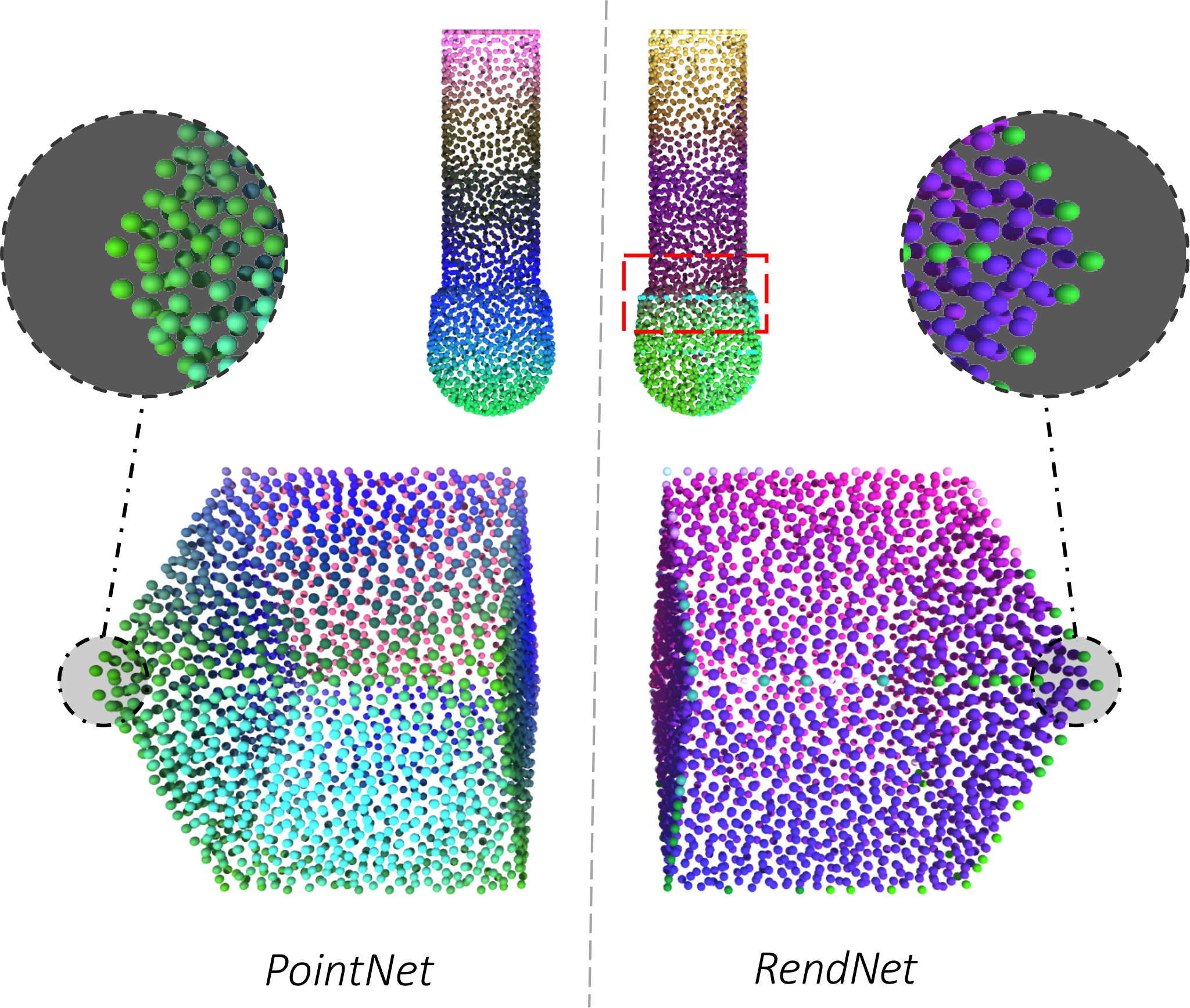
To investigate the representations learnt by RendNet, we trained a RendNet in an unsupervised manner with BYOL grill2020bootstrap on the ABC koch2019abc dataset. A PointNet qi2017pointnet is also trained under the same settings for comparison. We visualized the final point-wise representations by performing a Principal Component Analysis (PCA) to 3 dimensions and mapping them to RGB color components. The results are shown in Fig. 7. The upper object is a bolt. There is a fast change of representation for RendNet marked by the red box. Our representation differentiates the head and body of the bolt clearly. For the cubic object, both PointNet and RendNet emphasize edges and corners, but RendNet captures much sharper edges than PointNet. This means that RendNet is able to capture semantics more accurately.
5 Conclusion
In the paper, we propose RendNet, which leverages vector graphics and raster graphics to recognize 2D and 3D objects. We also design a new rendering method in latent space. Various experiments on 2D and 3D object recognition demonstrate that RendNet has higher performance and good efficiency compared with baselines. In the future, we can integrate more techniques to further improve the performance, such as pre-training on large VG datasets.
References
- (1) Emre Aksan, Thomas Deselaers, Andrea Tagliasacchi, and Otmar Hilliges. Cose: Compositional stroke embeddings. In NIPS, 2020.
- (2) Tadas Baltrušaitis, Chaitanya Ahuja, and Louis-Philippe Morency. Multimodal machine learning: A survey and taxonomy. IEEE transactions on pattern analysis and machine intelligence, 41(2):423–443, 2018.
- (3) Michael Bao, Matthew Cong, Stéphane Grabli, and Ronald Fedkiw. High-quality face capture using anatomical muscles. In Proceedings of the IEEE/CVF Conference on Computer Vision and Pattern Recognition, pages 10802–10811, 2019.
- (4) Alexey Bochkovskiy, Chien-Yao Wang, and Hong-Yuan Mark Liao. Yolov4: Optimal speed and accuracy of object detection. arXiv preprint arXiv:2004.10934, 2020.
- (5) Alexandre Carlier, Martin Danelljan, Alexandre Alahi, and Radu Timofte. Deepsvg: A hierarchical generative network for vector graphics animation. In NeurIPS, 2020.
- (6) Mathieu Delalandre, Ernest Valveny, and Jean-Yves Ramel. Recent contributions on the sesyd dataset for performance evaluation of symbol spotting systems.
- (7) Yifan Feng, Haoxuan You, Zizhao Zhang, Rongrong Ji, and Yue Gao. Hypergraph neural networks. In Proceedings of the AAAI Conference on Artificial Intelligence, volume 33, 2019.
- (8) Yaroslav Ganin, Sergey Bartunov, Yujia Li, Ethan Keller, and Stefano Saliceti. Computer-aided design as language. arXiv preprint arXiv:2105.02769, 2021.
- (9) Kyle Genova, Forrester Cole, Aaron Maschinot, Aaron Sarna, Daniel Vlasic, and William T Freeman. Unsupervised training for 3d morphable model regression. In Proceedings of the IEEE Conference on Computer Vision and Pattern Recognition, pages 8377–8386, 2018.
- (10) Justin Gilmer, Samuel S Schoenholz, Patrick F Riley, Oriol Vinyals, and George E Dahl. Neural message passing for quantum chemistry. In International conference on machine learning, pages 1263–1272. PMLR, 2017.
- (11) Ross Girshick. Fast r-cnn. In ICCV, 2015.
- (12) Ross Girshick, Jeff Donahue, Trevor Darrell, and Jitendra Malik. Rich feature hierarchies for accurate object detection and semantic segmentation. In CVPR, 2014.
- (13) Jean-Bastien Grill, Florian Strub, Florent Altché, Corentin Tallec, Pierre H. Richemond, Elena Buchatskaya, Carl Doersch, Bernardo Avila Pires, Zhaohan Daniel Guo, Mohammad Gheshlaghi Azar, Bilal Piot, Koray Kavukcuoglu, Rémi Munos, and Michal Valko. Bootstrap your own latent: A new approach to self-supervised learning, 2020.
- (14) Yulan Guo, Hanyun Wang, Qingyong Hu, Hao Liu, Li Liu, and Mohammed Bennamoun. Deep learning for 3d point clouds: A survey. IEEE TPAMI, 2021.
- (15) David Ha and Douglas Eck. A neural representation of sketch drawings. arXiv preprint arXiv:1704.03477, 2017.
- (16) Kaiming He, Xiangyu Zhang, Shaoqing Ren, and Jian Sun. Deep residual learning for image recognition. In CVPR, 2016.
- (17) Kaiming He, Xiangyu Zhang, Shaoqing Ren, and Jian Sun. Identity mappings in deep residual networks. In European conference on computer vision, pages 630–645. Springer, 2016.
- (18) Pradeep Kumar Jayaraman, Aditya Sanghi, Joseph G Lambourne, Karl DD Willis, Thomas Davies, Hooman Shayani, and Nigel Morris. Uv-net: Learning from boundary representations. In CVPR, 2021.
- (19) Xinyang Jiang, Lu Liu, Caihua Shan, Yifei Shen, Xuanyi Dong, and Dongsheng Li. Recognizing vector graphics without rasterization, 2021.
- (20) Hiroharu Kato, Deniz Beker, Mihai Morariu, Takahiro Ando, Toru Matsuoka, Wadim Kehl, and Adrien Gaidon. Differentiable rendering: A survey. arXiv preprint arXiv:2006.12057, 2020.
- (21) Thomas N. Kipf and Max Welling. Semi-supervised classification with graph convolutional networks. In ICLR, 2017.
- (22) Sebastian Koch, Albert Matveev, Zhongshi Jiang, Francis Williams, Alexey Artemov, Evgeny Burnaev, Marc Alexa, Denis Zorin, and Daniele Panozzo. Abc: A big cad model dataset for geometric deep learning. In CVPR, 2019.
- (23) Joseph G Lambourne, Karl DD Willis, Pradeep Kumar Jayaraman, Aditya Sanghi, Peter Meltzer, and Hooman Shayani. Brepnet: A topological message passing system for solid models. In CVPR, 2021.
- (24) Der-Tsai Lee and Bruce J Schachter. Two algorithms for constructing a delaunay triangulation. International Journal of Computer & Information Sciences, 9(3):219–242, 1980.
- (25) Tsung-Yi Lin, Piotr Dollár, Ross Girshick, Kaiming He, Bharath Hariharan, and Serge Belongie. Feature pyramid networks for object detection. In CVPR, 2017.
- (26) Tsung-Yi Lin, Priya Goyal, Ross Girshick, Kaiming He, and Piotr Dollár. Focal loss for dense object detection. In ICCV, 2017.
- (27) Hervé Locteau, Sébastien Adam, Eric Trupin, Jacques Labiche, and Pierre Héroux. Symbol spotting using full visibility graph representation. In Workshop on Graphics Recognition, 2007.
- (28) Raphael Gontijo Lopes, David Ha, Douglas Eck, and Jonathon Shlens. A learned representation for scalable vector graphics. In Proceedings of the IEEE/CVF International Conference on Computer Vision, pages 7930–7939, 2019.
- (29) Daniel Maturana and Sebastian Scherer. Voxnet: A 3d convolutional neural network for real-time object recognition. In IROS, 2015.
- (30) Amal Dev Parakkat, Marie-Paule R Cani, and Karan Singh. Color by numbers: Interactive structuring and vectorization of sketch imagery. In Proceedings of the 2021 CHI Conference on Human Factors in Computing Systems, pages 1–11, 2021.
- (31) Adam Paszke, Sam Gross, Soumith Chintala, Gregory Chanan, Edward Yang, Zachary DeVito, Zeming Lin, Alban Desmaison, Luca Antiga, and Adam Lerer. Automatic differentiation in pytorch. 2017.
- (32) Georgios Pavlakos, Luyang Zhu, Xiaowei Zhou, and Kostas Daniilidis. Learning to estimate 3d human pose and shape from a single color image. In Proceedings of the IEEE Conference on Computer Vision and Pattern Recognition, pages 459–468, 2018.
- (33) Charles R Qi, Hao Su, Kaichun Mo, and Leonidas J Guibas. Pointnet: Deep learning on point sets for 3d classification and segmentation. In Proceedings of the IEEE conference on computer vision and pattern recognition, pages 652–660, 2017.
- (34) Charles R Qi, Li Yi, Hao Su, and Leonidas J Guibas. Pointnet++: Deep hierarchical feature learning on point sets in a metric space. NeurIPS, 2017.
- (35) Jean-Yves Ramel, Nicole Vincent, and Hubert Emptoz. A structural representation for understanding line-drawing images. IJDAR, 2000.
- (36) Pradyumna Reddy, Michael Gharbi, Michal Lukac, and Niloy J Mitra. Im2vec: Synthesizing vector graphics without vector supervision. arXiv preprint arXiv:2102.02798, 2021.
- (37) Joseph Redmon and A.Farhadi. Yolov3: An incremental improvement. arXiv preprint arXiv:1804.02767, 2018.
- (38) Joseph Redmon, Santosh Divvala, Ross Girshick, and Ali Farhadi. You only look once: Unified, real-time object detection. In CVPR, 2016.
- (39) Joseph Redmon and Ali Farhadi. Yolo9000: better, faster, stronger. In CVPR, 2017.
- (40) Shaoqing Ren, Kaiming He, Ross Girshick, and Jian Sun. Faster r-cnn: towards real-time object detection with region proposal networks. IEE TPAMI, 2016.
- (41) Helge Rhodin, Nadia Robertini, Christian Richardt, Hans-Peter Seidel, and Christian Theobalt. A versatile scene model with differentiable visibility applied to generative pose estimation. In Proceedings of the IEEE International Conference on Computer Vision, pages 765–773, 2015.
- (42) KC Santosh, Bart Lamiroy, and Laurent Wendling. Symbol recognition using spatial relations. Pattern Recognition Letters, 2012.
- (43) I-Chao Shen and Bing-Yu Chen. Clipgen: A deep generative model for clipart vectorization and synthesis. IEEE Transactions on Visualization and Computer Graphics, 2021.
- (44) Hang Su, Subhransu Maji, Evangelos Kalogerakis, and Erik Learned-Miller. Multi-view convolutional neural networks for 3d shape recognition. In ICCV, 2015.
- (45) Chien-Yao Wang, Alexey Bochkovskiy, and Hong-Yuan Mark Liao. Scaled-yolov4: Scaling cross stage partial network. arXiv preprint arXiv:2011.08036, 2020.
- (46) Minjie Wang, Da Zheng, Zihao Ye, Quan Gan, Mufei Li, Xiang Song, Jinjing Zhou, Chao Ma, Lingfan Yu, Yu Gai, et al. Deep graph library: A graph-centric, highly-performant package for graph neural networks. arXiv preprint arXiv:1909.01315, 2019.
- (47) Yansen Wang, Zhen Fan, and Carolyn Rose. Incorporating multimodal information in open-domain web keyphrase extraction. In Proceedings of the 2020 Conference on Empirical Methods in Natural Language Processing (EMNLP), pages 1790–1800, 2020.
- (48) Yue Wang, Yongbin Sun, Ziwei Liu, Sanjay E Sarma, Michael M Bronstein, and Justin M Solomon. Dynamic graph cnn for learning on point clouds. ACM TOG, 2019.
- (49) Xin Wei, Ruixuan Yu, and Jian Sun. View-gcn: View-based graph convolutional network for 3d shape analysis. In CVPR, 2020.
- (50) Wenxuan Wu, Zhongang Qi, and Li Fuxin. Pointconv: Deep convolutional networks on 3d point clouds. In Proceedings of the IEEE/CVF Conference on Computer Vision and Pattern Recognition, pages 9621–9630, 2019.
- (51) Siyuan Xiang, Ching Tseng, Congcong Wen, Deshana Desai, Yifeng Kou, Binil Starly, Daniele Panozzo, and Chen Feng. Cluster3d: A dataset and benchmark for clustering non-categorical 3d cad models. 2021.
- (52) Cem Yuksel. Sample elimination for generating poisson disk sample sets. In Computer Graphics Forum, volume 34, pages 25–32. Wiley Online Library, 2015.
- (53) Amir Zadeh, Minghai Chen, Soujanya Poria, Erik Cambria, and Louis-Philippe Morency. Tensor fusion network for multimodal sentiment analysis. In Proceedings of the 2017 Conference on Empirical Methods in Natural Language Processing, pages 1103–1114, 2017.
- (54) Zhibo Zhang, Prakhar Jaiswal, and Rahul Rai. Featurenet: Machining feature recognition based on 3d convolution neural network. Computer-Aided Design, 101:12–22, 2018.
- (55) Yin Zhou and Oncel Tuzel. Voxelnet: End-to-end learning for point cloud based 3d object detection. In CVPR, 2018.