Fast and Safe Aerial Payload Transport in Urban Areas

Aeris El Asslouj , Harshvardhan Uppaluru and Hossein Rastgoftar Note: Student, Electrical and Computer Engineering Department, University of Arizona, Email: aymaneelasslouj@email.arizona.edu. Note: PhD Student, Aerospace and Mechanical Engineering Department, University of Arizona, Email: huppaluru@email.arizona.edu. Note: Assistant Professor, Aerospace and Mechanical Engineering Department, University of Arizona, Email: hrastgoftar@arizona.edu.

Abstract

This paper studies the problem of fast and safe aerial payload transport by a single quadcopter in urban areas. The quadcopter payload system (QPS) is considered as a rigid body and modeled with a nonlinear dynamics. The urban area is modeled as an obstacle-laden environment with obstacle geometries obtained by incorporating realistic LIDAR data. Our approach for payload transport is decomposed into high-level motion planning and low-level trajectory control. For the low-level trajectory tracking, a feedback linearization control is applied to stably track the desired trajectory of the quadcopter. For high-level motion planning, we integrate A* search and polynomial planning to define a safe trajectory for the quadcopter assuring collision avoidance, boundedness of the quadcopter rotor speeds and tracking error, and fast arrival to a target destination from an arbitrary initial location.

1 Nomenclature

$s_{i}$ =	Angular speed of rotor $i$ ( $i=1,2,3,4$ )
$s_{max}$ =	Maximum rotor speed
$\mathbf{r}_{i}$ =	Initial position
$\mathbf{r}_{f}$ =	Target position
$\mathbf{r}(t)$ =	Actual trajectory
$\mathbf{p}(t)$ =	Desired trajectory
$\delta$ =	Tracking error upper bound
$\phi$ , $\theta$ , $\psi$ =	Roll, pitch, and yaw angles of the quadcopter
$m$ =	Quadcopter mass
$\mathbf{J}$ =	Mass moment of inertia of the quadcopter
$\mathbf{S}$ =	Rotation matrix
$\hat{\mathbf{e}}_{1}$ , $\hat{\mathbf{e}}_{2}$ , $\hat{\mathbf{e}}_{2}$ =	Bases of the inertial coordinate system
$\hat{\mathbf{b}}_{1}$ , $\hat{\mathbf{b}}_{2}$ , $\hat{\mathbf{b}}_{2}$ =	Bases of the quadcopter body coordinate system
$\boldsymbol{\omega}$ =	Quadcopter angular velocity

2 Introduction

Over the past two decades, quadcopters has become increasingly affordable and widely used for military and non-military applications due to their high performance, maneuverability and dynamic simplicity. Applications of quadcopters include remote sensing, firefighting, traffic surveillance tasks [1, 2], search and rescue operations [3, 4, 5], wildlife monitoring and exploration [6] and educational purposes. Aerial payload transportation is one such interesting application commonly used in construction, military response, emergency response, and delivery tasks [7, 8]. Typically, for cases when the payload is not heavy, a single quadcopter can carry the payload via a single cable attached between quadcopter and payload. This is particularly useful in remote areas with uneven terrains where it is difficult to secure a safe landing place.

2.1 Related Work

Previously, the area of payload transport has been extensively studied for helicopters [9, 10]. The dynamics, stabilization, and control of a payload carrying helicopter were modeled in [11, 10, 12]. So far, single quadcopter or multiple quadcopters have been considered for payload transport and deployment [13, 14, 15, 16, 17, 18] due to their high thrust generation capabilities. Generally, there are two means of payload transportation carried out by quadcopters, i.e., active and passive attachments, each having their own advantages and disadvantages. The passive approach uses a suspended cable [19, 20, 21] with one end attached to the quadcopter and the load is attached to the other end. However, this approach is not feasible in outdoor environments and the controller design becomes more complex due to additional degree of under-actuation. Since most passive approaches are based on the common assumption that the suspended cable is always taut, their applications are restricted. Active approach adds an additional degree of freedom that requires a gripper to grasp at the payload and provides a better solution especially in constrained altitudes.

Aerial payload transportation and manipulation using a single quadcopter was studied [22, 23, 24, 25, 20]. Stabilization of a single quadcopter carrying a single payload was also analyzed [26, 27], Researcher have proposed H^∞ control [24], and PID control [28] for a quadcopter carrying a suspended payload. A quadcopter carrying payload with varying length cable was studied [25]. For emergency response, commercial and military applications, cooperative aerial payload transportation and manipulation has been considered [29, 22, 30, 31]

2.2 Contributions and Outline

This paper proposes a multi-layer approach for safe and fast transportation of an aerial payload carried by a single quadcopter in an urban area. We assume that the quadcopter and payload together act as a rigid body and is known as quadcopter payload system (QPS). QPS is modeled by $14$ -th order nonlinear dynamics whereas the environment is modeled using geometry from LIDAR data. We tested our algorithm and controller in a simulation with a sample payload transport mission through the University of Arizona and presented the results in 7. We used The United States Geological Survey (USGS)’s Lidar data to create the simulation environment in a manner that is widely applicable in the United States as the USGS’s Lidar data covers most of the country. Compared with the existing literature, our proposed payload transportation solution offers the following contributions:

1.

high-level motion planning that integrates A* search and polynomial planning to obtain safe trajectory of the QPS minimizing travel distance from an initial position to a target destination.
2.

low-level trajectory tracking control ensuring stability and boundedness of rotor angular speeds and tracking error in a general payload transportation mission in an obstacle-laden environment with arbitrary distributions of obstacles.

This paper is organized as follows: The problem statement is defined in Section 3. Section 4 describes the model of the environment and the quadrotor payload system. Section 5 discusses the mathematical modeling of quadcopters and trajectory tracking control. Section 6 presents the high-level motion planning approach used for simulations. We finally present our simulation results using the described model and control in Section 7 before putting forward our concluding remarks in Section 8.

3 Problem Statement

We consider a quadcopter carrying a payload in an urban area with given initial position $\mathbf{r}_{i}$ and target position $\mathbf{r}_{f}$ . The QPS is enclosed by a sphere of radius $\epsilon$ and follows the nonlinear dynamics presented in Section 4.2. The environment is made up of free space and obstacle space (i.e terrain and structures) as described in Section 4.1.

This paper develops a pair of algorithms to choose a valid desired trajectory $\mathbf{p}(t)$ in Section 6. They include A*-based algorithm for spatial planning to keep desired trajectory $\mathbf{p}(t)$ collision-free, and a bi-section-based algorithm for temporal planning of $\mathbf{p}(t)$ to minimize mission time. Then, a feedback linearization controller will be applied in Section 5 to compute rotor speeds that allow the system to track the desired trajectory while respecting the following safety conditions:

Bounded Rotor Speed: The rotor angular speeds of the quadcopter, denoted by $s_{1}$ through $s_{4}$ need to satisfy the safety requirement

\bigwedge_{j=1}^{4}\left(0\leq s_{j}\left(t\right)\leq s_{max}\right),\qquad\forall t,

(1)

where $s_{max}$ is the maximum angular speed for all quadcopter rotors, and “ $\bigwedge$ ” means “include all”.

Bounded Trajectory Tracking: It is required to assure that the tracking error remains bounded at any time $t$ . This condition can be formally specified by

\|\mathbf{r}(t)-\mathbf{p}(t)\|\leq\delta,\qquad\forall t,

(2)

where $\delta$ is the tracking bound and $\mathbf{r}(t)$ is the actual trajectory of the QPS.

Obstacle Collision Avoidance Guarantee: It is required to guarantee that the QPS does not hit any structure or terrain in the urban area. This is formally specified as

\|\mathbf{r}(t)-\mathbf{o}\|>\epsilon,\qquad\forall\mathbf{o}\in\mathbf{Obstacle\ space},\qquad\forall t,

(3)

where $\mathbf{Obstacle\ space}$ is the space occupied by either the terrain or structures.

4 Modeling

We first define the model of the environment in Section 4.1 and the model of the QPS in Section 4.2. In Section 4.2, we also derive a set of formulas to compute desired rotor speeds that guarantee a desired thrust and a desired Euler acceleration.

4.1 Environment model

The environment is modeled as a continuous three-dimensional space $\mathbf{Environment}$ with coordinate system $\left(x,y,z\right)$ . The environment is split by an elevation map $M$ into $\mathbf{Free\ space}$ above it and $\mathbf{Obstacle\ space}$ under it. This representation is easier to process and only requires altitude data but does not allow for crossing under structures. It can be formalized as:

	$M:(x,y)\rightarrow\text{highest terrain or structure altitude at (x,y)},\qquad\forall(x,y,z)\in\mathbf{Environment},$		(4a)
	$\mathbf{Obstacle\ space}=\left\{(x,y,z)\in\mathbf{Environment}\ \|\ z<M(x,y)\right\},$		(4b)
	$\mathbf{Free\ space}=\left\{(x,y,z)\in\mathbf{Environment}\ \|\ z>M(x,y)\right\}.$		(4c)

To ensure that the system remains at a distance of $\epsilon+\delta$ from the obstacle space, we expand the elevation map $M$ into an expanded elevation map $M_{E}$ . This is done by taking each point of the surface formed by the elevation map in three dimensional space and translating it in the local upward normal direction by a distance of $\epsilon+\delta$ . If we define $\mathbf{S_{M}}$ and $\mathbf{Exp(S_{M})}$ as respectively the three dimensional surface of the elevation map and its expanded version, we can write

\mathbf{Exp(S_{M})}=\left\{(x,y,z)+(\epsilon+\delta)\hat{\mathbf{n}}_{\mathbf{S_{M}}}(x,y)\ |\ (x,y,z)\in\mathbf{S_{M}}\right\},

(5)

where $\hat{\mathbf{n}}_{\mathbf{S_{M}}}(x,y)$ is the unit normal of $\mathbf{S_{M}}$ at $(x,y)$ such that:

\hat{\mathbf{n}}_{\mathbf{S_{M}}}(x,y)=\frac{1}{\left\lVert\begin{bmatrix}-\frac{\partial M}{\partial x}&-\frac{\partial M}{\partial y}&1\end{bmatrix}\right\rVert}\begin{bmatrix}-\frac{\partial M}{\partial x}&-\frac{\partial M}{\partial y}&1\end{bmatrix}.

(6)

The expanded elevation map $M_{E}$ is defined as the highest point of the expanded elevation surface $\mathbf{Exp(S_{M})}$ :

M_{E}:(x,y)\rightarrow max\left\{z\ |\ (x,y,z)\in\mathbf{Exp(S_{M})}\right\}.

(7)

Note that because of this, $\mathbf{Exp(S_{M})}$ is not necessarily the surface $\mathbf{S_{M_{E}}}$ formed by $M_{E}$ in three dimensional space.

In a similar fashion to $M$ , $M_{E}$ splits $\mathbf{Environment}$ into $\mathbf{Restricted\ free\ space}$ above it and $\mathbf{Expanded\ obstacle\ space}$ under it:

	$\mathbf{Expanded\ obstacle\ space}=\left\{(x,y,z)\in\mathbf{Environment}\ \|\ z<M_{E}(x,y)\right\},$		(8a)
	$\mathbf{Restricted\ free\ space}=\left\{(x,y,z)\in\mathbf{Environment}\ \|\ z>M_{E}(x,y)\right\}.$		(8b)

4.2 Quadcopter-payload system (QPS) model

Refer to caption — Figure 1: QPS model with rotor angular speeds $s_{1}$ through $s_{4}$ , rotor arm length $l$ , and frame $(\hat{\mathbf{b}}_{1},\hat{\mathbf{b}}_{2},\hat{\mathbf{b}}_{3})$

We use the kinematics and dynamics presented in Sections 4.2.1 and 4.2.2 to model the motion of the QPS in an urban area.

4.2.1 Kinematics

To characterize the rotation of the QPS, we fix a body frame at the center of mass of the QPS with the schematic shown in Fig. 1 , and apply the $3-2-1$ Euler angle standard as shown in Fig. 2 to characterize the rotation of the QPS with respect to the inertial coordinate system which is specified by matrix

\mathbf{S}\left(\phi,\theta,\psi\right)=\begin{bmatrix}\cos{\theta}\cos{\psi}&\cos{\theta}\sin{\psi}&-\sin{\theta}\\ \sin{\phi}\sin{\theta}\cos{\psi}-\cos{\phi}\sin{\psi}&\sin{\phi}\sin{\theta}\sin{\psi}+\cos{\phi}\cos{\psi}&\sin{\phi}\cos{\theta}\\ \cos{\phi}\sin{\theta}\cos{\psi}+\sin{\phi}\sin{\psi}&\cos{\phi}\sin{\theta}\sin{\psi}-\sin{\phi}\cos{\psi}&\cos{\phi}\cos{\theta}\end{bmatrix},

where $\phi$ , $\theta$ , and $\psi$ are the roll, pitch, and yaw angles. The QPS body axes are denoted by $\hat{\mathbf{b}}_{1}$ , $\hat{\mathbf{b}}_{2}$ , and $\hat{\mathbf{b}}_{3}$ and related to the base vectors of the inertial coordinate system by

\hat{\mathbf{b}}_{h}(t)=\mathbf{S}^{T}\left(\phi,\theta,\psi\right)\hat{\mathbf{e}}_{h},\qquad~h=1,2,3.

(9)

To obtain the angular velocity and angular acceleration of the QPS, we define two intermediate coordinate transformations with bases $\left(\hat{\mathbf{c}}_{1},\hat{\mathbf{c}}_{2},\hat{\mathbf{c}}_{3}\right)$ and $\left(\hat{\mathbf{d}}_{1},\hat{\mathbf{d}}_{2},\hat{\mathbf{d}}_{3}\right)$ that are defined as follows:

	$\hat{\mathbf{c}}_{h}(t)=\mathbf{S}^{T}\left(0,0,\psi\right)\hat{\mathbf{e}}_{h},\qquad~h=1,2,3.$		(10a)
	$\hat{\mathbf{d}}_{h}(t)=\mathbf{S}^{T}\left(0,\theta,\psi\right)\hat{\mathbf{e}}_{h},\qquad~h=1,2,3.$		(10b)

The angular velocity and acceleration of the QPS are then obtained as follows [32]:

	${\boldsymbol{\omega}}=\dot{\psi}\hat{\mathbf{c}}_{3}+\dot{\theta}\hat{\mathbf{d}}_{2}+\dot{\phi}_{i}\hat{\mathbf{b}}_{1},$		(11a)
	$\dot{{\boldsymbol{\omega}}}=\ddot{\psi}\hat{\mathbf{c}}_{3}+\ddot{\theta}\hat{\mathbf{d}}_{2}+\ddot{\phi}_{i}\hat{\mathbf{b}}_{1}+\dot{\theta}\dot{\psi}\hat{\mathbf{c}}_{3}\times\hat{\mathbf{d}}_{2}+\dot{\phi}\left(\dot{\psi}\hat{\mathbf{c}}_{3}+\dot{\theta}\hat{\mathbf{d}}_{2}\right)\times\hat{\mathbf{b}}_{1}$		(11b)

4.2.2 Dynamics

By applying the Newton’s second law, the translational dynamics of the QPS is obtained by

m\ddot{\mathbf{r}}=p\hat{\mathbf{b}}_{3}-mg\hat{\mathbf{e}}_{3}

(12)

where $m$ is the total mass of the QPS, $p$ is the magnitude of the thrust force generated by the rotors, and $g=9.81m/s^{2}$ is the gravitational acceleration. To obtain the rotational dynamics, we notice that the QPS is symmetrically distributed around the $\hat{\mathbf{b}}_{3}$ axis and is symmetric with respect to the $\hat{\mathbf{b}}_{3}-\hat{\mathbf{b}}_{1}$ and $\hat{\mathbf{b}}_{2}-\hat{\mathbf{b}}_{3}$ planes. Therefore, the mass moment of inertia of the QPS is diagonal and positive definite and denoted by $\mathbf{J}$ when it is realized with respect to the QPS body frame. The rotational dynamics of the QPS is then obtained by

\mathbf{J}\dot{{\boldsymbol{\omega}}}=-{\boldsymbol{\omega}}\times\mathbf{J}{\boldsymbol{\omega}}+\boldsymbol{\tau},

(13)

where $\boldsymbol{\tau}$ is the control torque expressed with respect to the inertial coordinate system.

Rotor Angular Speeds:

To obtain the rotor angular speeds, we first express control torque vector $\boldsymbol{\tau}$ with respect to the QPS body frame as follows:

\boldsymbol{\tau}_{B}=\mathbf{S}\left(\phi,\theta,\psi\right)\boldsymbol{\tau},

(14)

where $\boldsymbol{\tau}_{B}=\begin{bmatrix}\tau_{\phi}&\tau_{\theta}&\tau_{\psi}\end{bmatrix}^{T}$ . Then, based on Fig. 1, squares of rotor angular speeds, denoted by $s_{1}^{2}$ , $s_{2}^{2}$ , $s_{3}^{2}$ , and $s_{4}^{2}$ , can be related to $p$ , $\tau_{\phi}$ , $\tau_{\theta}$ , and $\tau_{\psi}$ with []

\begin{bmatrix}s_{1}^{2}\\ s_{2}^{2}\\ s_{3}^{2}\\ s_{4}^{2}\end{bmatrix}=\begin{bmatrix}b&b&b&b\\ 0&-bl&0&bl\\ -bl&0&bl&0\\ -k&k&-k&k\end{bmatrix}^{-1}\begin{bmatrix}p\\ \tau_{\phi}\\ \tau_{\theta}\\ \tau_{\psi}\end{bmatrix}

(15)

where $b>0$ and $k>0$ are aerodynamics coefficients and $l>0$ is the length of the quadcopter arm.

5 Control

By extending the translational and rotational dynamics of the quadcopter, the motion of the quadcopter can be modeled by

\begin{cases}\dot{\mathbf{x}}=\mathbf{f}\left(\mathbf{x}\right)+\mathbf{G}\mathbf{u}\\ \mathbf{y}=\begin{bmatrix}x&y&z&\psi\end{bmatrix}^{T}\end{cases},

(16)

where $\mathbf{y}$ is the output vector, and

	$\mathbf{x}=\begin{bmatrix}x&y&z&\dot{x}&\dot{y}&\dot{z}&\phi&\theta&\psi&\dot{\phi}&\dot{\theta}&\dot{\psi}&p&\dot{p}\end{bmatrix}^{T},$		(17a)
	$\mathbf{u}=\begin{bmatrix}u_{1}&u_{2}&u_{3}&u_{4}\end{bmatrix}^{T}=\begin{bmatrix}\ddot{p}&\ddot{\phi}&\ddot{\theta}&\ddot{\psi}\end{bmatrix}^{T},$		(17b)

are the state vector and the control input of the quadcopter respectively. In (16),

	$\mathbf{f}\left(\mathbf{x}\right)=\begin{bmatrix}\dot{x}&\dot{y}&\dot{z}&\left({\frac{p}{m}\hat{\mathbf{b}}_{3}-{g}\hat{\mathbf{e}}_{3}}\right)^{T}&\dot{\phi}&\dot{\theta}&\dot{\psi}&0&0&0&\dot{p}&0\end{bmatrix}^{T},$		(18a)
	$\mathbf{G}=\begin{bmatrix}\mathbf{0}_{9\times 1}&\mathbf{0}_{9\times 3}\\ \mathbf{0}_{3\times 1}&\mathbf{I}_{3}\\ 0&\mathbf{0}_{1\times 3}\\ 1&\mathbf{0}_{1\times 3}\\ \end{bmatrix},$		(18b)

are smooth functions obtained in Ref. [32], where $\mathbf{I}_{3}\in\mathbb{R}^{3\times 3}$ is the identity matrix, $\mathbf{0}_{3\times 1}\in\mathbb{R}^{3\times 1}$ , $\mathbf{0}_{3\times 3}\in\mathbb{R}^{3\times{3}}$ , and $\mathbf{0}_{3\times 9}\in\mathbb{R}^{3\times{9}}$ are the zero-entry matrices. We use the input-state feedback linearization approach, presented in [32], for low-level trajectory tracking. To this end, we use state transformation $\mathbf{z}=\mathbf{z}\left(\mathbf{x}\right)$

\mathbf{z}(\mathbf{x})=\begin{bmatrix}x&y&z&\dot{x}&\dot{y}&\dot{z}&\ddot{x}&\ddot{y}&\ddot{z}&\dddot{x}&\dddot{y}&\dddot{z}&\psi&\dot{\psi}\end{bmatrix}^{T}.

(19)

Proposition 1.

There is a one-to-one transformation between $\mathbf{x}$ and $\mathbf{z}$ .

Proof.

Note that $x$ , $y$ , $z$ , $\dot{x}$ , $\dot{y}$ , $\dot{z}$ , $\psi$ , and $\dot{\psi}$ are the components of vectors $\mathbf{x}$ and $\mathbf{z}$ , and the remaining components of $\mathbf{z}$ , $\ddot{x}$ , $\ddot{y}$ , $\ddot{z}$ , $\dddot{x}$ , $\dddot{y}$ , and $\dddot{z}$ , can be obtained based on components of state vector $\mathbf{x}$ as follows:

\begin{bmatrix}\ddot{x}&\ddot{y}&\ddot{z}&\dddot{x}&\dddot{y}&\dddot{z}\end{bmatrix}^{T}=\mathbf{h}\left(p,\phi,\theta,\psi,\dot{p},\dot{\phi},\dot{\theta},\dot{\psi}\right)=\frac{1}{m}\begin{bmatrix}-{mg}\hat{\mathbf{e}}_{3}+{p}\hat{\mathbf{b}}_{3}\\ {\dot{p}}\hat{\mathbf{b}}_{3}+p\left({\boldsymbol{\omega}}\times\hat{\mathbf{b}}_{3}\right)\end{bmatrix}.

(20)

On the other hand, $\psi$ , $p$ , $\phi$ , and $\theta$ can be obtained based on $\ddot{x}$ , $\ddot{y}$ , and $\ddot{z}$ . Also, by taking time derivative from acceleration vector $\ddot{\mathbf{r}}$ , we can write

\dddot{\mathbf{r}}=\frac{1}{m}\dot{p}\hat{\mathbf{b}}_{3}+\frac{p}{m}\left({\boldsymbol{\omega}}\times\hat{\mathbf{b}}_{3}\right)=\begin{bmatrix}\frac{1}{m}\hat{\mathbf{b}}_{3}&-\frac{p}{m}\hat{\mathbf{b}}_{2}&\frac{p}{m}\hat{\mathbf{d}}_{2}\times\hat{\mathbf{b}}_{3}\end{bmatrix}\begin{bmatrix}\dot{p}&\dot{\phi}&\dot{\theta}\end{bmatrix}^{T}+\frac{p}{m}\dot{\psi}\hat{\mathbf{c}}_{3}\times\hat{\mathbf{b}}_{3}

Therefore, $\dot{p}$ , $\dot{\phi}$ , and $\dot{\theta}$ are obtained by

\begin{bmatrix}\dot{p}&\dot{\phi}&\dot{\theta}\end{bmatrix}^{T}=\begin{bmatrix}\frac{1}{m}\hat{\mathbf{b}}_{3}&-\frac{p}{m}\hat{\mathbf{b}}_{2}&\frac{p}{m}\hat{\mathbf{d}}_{2}\times\hat{\mathbf{b}}_{3}\end{bmatrix}^{-1}\left(\begin{bmatrix}\dddot{x}&\dddot{y}&\dddot{z}\end{bmatrix}^{T}-\frac{p}{m}\dot{\psi}\hat{\mathbf{c}}_{3}\times\hat{\mathbf{b}}_{3}\right)

(21)

∎

Note that $\mathbf{z}$ is updated by

\dot{\mathbf{z}}=\mathbf{A}\mathbf{z}+\mathbf{B}\mathbf{v}

(22)

with

	$\mathbf{A}=\begin{bmatrix}\mathbf{0}_{9\times 3}&\mathbf{I}_{9}&\mathbf{0}_{9\times 1}&\mathbf{0}_{9\times 1}\\ \mathbf{0}_{3\times 3}&\mathbf{0}_{3\times 9}&\mathbf{0}_{3\times 1}&\mathbf{0}_{3\times 1}\\ \mathbf{0}_{1\times 3}&\mathbf{0}_{1\times 9}&0&1\\ \mathbf{0}_{1\times 3}&\mathbf{0}_{1\times 9}&0&0\\ \end{bmatrix},$		(23a)
	$\mathbf{B}=\begin{bmatrix}\mathbf{0}_{9\times 3}&\mathbf{0}_{9\times 1}\\ \mathbf{I}_{3}&\mathbf{0}_{3\times 1}\\ \mathbf{0}_{1\times 3}&0\\ \mathbf{0}_{1\times 3}&1\\ \end{bmatrix},$		(23b)

where $\mathbf{v}=\begin{bmatrix}\ddddot{x}&\ddddot{y}&\ddddot{z}&\ddot{\psi}\end{bmatrix}^{T}$ is related to $\mathbf{u}$ by

\mathbf{v}=\mathbf{M}\mathbf{u}+\mathbf{N},

(24)

where

	$\mathbf{M}=\left[\begin{array}[]{ccc\|c}\frac{1}{m}\hat{\mathbf{b}}_{3}&-\frac{p}{m}\hat{\mathbf{b}}_{2}&\frac{p}{m}\hat{\mathbf{d}}_{2}\times\hat{\mathbf{b}}_{3}&\frac{p}{m}\hat{\mathbf{c}}_{3}\times\hat{\mathbf{b}}_{3}\\ \hline\cr 0&0&0&1\end{array}\right],$		(25a)
	$\mathbf{N}=\dot{\theta}\dot{\psi}\left(\hat{\mathbf{c}}_{3}\times\hat{\mathbf{d}}_{2}\right)+\dot{\phi}\left(\dot{\psi}\hat{\mathbf{c}}_{3}+\dot{\theta}\hat{\mathbf{d}}_{2}\right)\times\hat{\mathbf{b}}_{1}.$		(25b)

Trajectory Control Design: We choose

\mathbf{v}=\mathbf{K}\left(\mathbf{z}_{d}-\mathbf{z}\right)

(26)

where $\mathbf{K}$ is the control gain matrix and $\mathbf{z}_{d}(t)=\begin{bmatrix}\mathbf{p}^{T}(t)&\dot{\mathbf{p}}^{T}(t)&\ddot{\mathbf{p}}^{T}(t)&\dddot{\mathbf{p}}^{T}(t)&\psi_{d}(t)&\dot{\psi}_{d}(t)\end{bmatrix}^{T}$ is the desired state at time $t$ (see Figure 3). Without loss of generality, we choose $\psi_{d}(t)=0$ and $\dot{\psi}_{d}(t)=0$ at any time $t$ . We propose a spatiotemporal approach in Section 6 to obtain desired trajectory $\mathbf{p}\left(t\right)$ that is differentiable and bounded at any time $t$ . The state vector $\mathbf{z}$ is updated by

\dot{\mathbf{z}}=\left(\mathbf{A}-\mathbf{B}\mathbf{K}\right)\mathbf{z}+\mathbf{K}\mathbf{z}_{d}

(27)

We choose control gain matrix $\mathbf{K}$ such that matrix $\mathbf{A}-\mathbf{B}\mathbf{K}$ is Hurwitz. Then, the dynamics (27) is Bounded-Input-Bounded-Output (BIBO) stable [33].

6 Planning

We first implement the A* (A star) path-finding algorithm in Section 6.1 to find a piece-wise straight path which ensures that the system moves from the initial position to the final position while respecting safety condition (3). Then, we implement a bi-section algorithm in Section 6.2 to find the minimum time required for the QPS to execute each part of the path while respecting safety conditions (1) and (2).

6.1 Spatial planning

To find a path from the initial position to the final position, that respects the obstacle safety condition, this paper proposes using the weighted A* algorithm with an exploration grid that is dynamically generated. To implement the A* search, we discretize the environment with resolution $\Delta$ through the following pairs of functions:

	$\mathbf{F}:(x,y,z)\rightarrow\left(\left\lfloor\frac{x}{\Delta}+\frac{1}{2}\right\rfloor,\left\lfloor\frac{y}{\Delta}+\frac{1}{2}\right\rfloor,\left\lfloor\frac{z}{\Delta}+\frac{1}{2}\right\rfloor\right),\quad\forall(x,y,z)\in\mathbf{Environment},$		(28a)
	$\mathbf{F^{-1}}:(i,j,k)\rightarrow\left(\Delta\times i,\Delta\times j,\Delta\times k\right).\quad\forall(i,j,k)\in F\left(\mathbf{Environment}\right).$		(28b)

Equation (28a) converts continuous-valued point $\left(x,y,z\right)$ to discrete valued point $\left(i,j,k\right)$ . On the other hand, Eq. (28b) converts dicrete-valued $(i,j,k)$ to an associated discrete-valued point in the environment. We perform the following steps to spatially plan a safe path from the initial position to the target destination:

Convert the initial position $\mathbf{r}_{i}=\begin{bmatrix}x_{i}&y_{i}&z_{i}\end{bmatrix}^{T}$ , final position $\mathbf{r}_{f}=\begin{bmatrix}x_{f}&y_{f}&z_{f}\end{bmatrix}^{T}$ , and expanded elevation map $M_{E}$ to initial index, final index, and discrete expanded elevation map $M_{E}^{\prime}$ using Function (28a).

	$(i_{1},j_{1},k_{1})=\mathbf{F}(x_{i},y_{i},z_{i}),\quad(i_{N},j_{N},k_{N})=\mathbf{F}(x_{f},y_{f},z_{f}),$		(29a)
	$M_{E}^{\prime}:(i,j)\rightarrow\max\left(\left\{k\ \|\ (i,j,k)\in\mathbf{F(Expanded\ obstacle\ space)}\right\}\right).$		(29b)

Note that (29b) defines the discrete expanded elevation map as taking the maximum value in the area covered by indices i and j. And that $N\in\mathbb{N}$ is a finite free variable determined by solving the A* search.

2.

Run Algorithm 1 with resolution $\Delta$ and weight $w$ . The output is a sequence of $N$ indices $\left(i_{n},j_{n},k_{n}\right)$ with $n\in\left\{1,\cdots,N\right\}$ that, when connected with segments, form a collision-free path from the initial index to the final index within the grid of resolution $\Delta$ .

Convert back this sequence of indices to obtain a sequence of $N$ points $\bar{\mathbf{p}}_{n}$ using Function (28b). These points form a piece-wise straight path between the initial position and the final position which respects the obstacle safety condition as it is contained within the $\mathbf{Restricted\ free\ space}$ . This desired trajectory $\mathbf{p}$ is parameterized with parameter $u$ such that:

	$\bar{\mathbf{p}}_{n}=\mathbf{F^{-1}}(i_{n},j_{n},k_{n})\quad\forall n\in\left\{1,\cdots,N\right\},$		(30a)
	$\mathbf{p}(u)=\begin{cases}\bar{\mathbf{p}}_{n}+(u-n)\times\left(\bar{\mathbf{p}}_{n+1}-\bar{\mathbf{p}}_{n}\right)\quad n\leq u<n+1\quad\forall n\in\left\{1,\cdots,(N-1)\right\}.\end{cases}$		(30b)

Algorithm 1 Weighted A* search algorithm with dynamically generated grid

Initial_index, Final_index,

M_{E}^{\prime}

\Delta

, and

w

Path is a list of connected indices from initial index to final index through

\mathbf{F(Restricted\ free\ space)}

index: [integer, integer, integer]

\triangleright

identifies a cell with indices i, j, and k

node: [index, real number]

\triangleright

is a cell with the index of the previous node

OpenSet

\leftarrow

HashTable<index,node> and the distance from the initial node

ClosedSet

\leftarrow

HashTable<index,node>

OpenSet[Initial_index]

\leftarrow

[None, 0]

while OpenSet.keys

\neq\emptyset

\wedge

Final_index

\notin

ClosedSet.keys do

PickedIndex

\leftarrow

min(OpenSet.keys, Index

\rightarrow

OpenSet[Index][1] +

w\times

distance(Index,Final_index))

\triangleright

Pick the open node with the lowest total cost

Neighbors

\leftarrow

neighbors(PickedIndex)

\triangleright

Get neighbors of the picked node

Neighbors

\leftarrow

[Neighbor

\in

Neighbors

|

Neighbor

\notin

ClosedSet.keys]

\triangleright

Filter out closed neighbors

Neighbors

\leftarrow

[Neighbor

\in

Neighbors

|

Neighbor[2] >

M_{E}^{\prime}

(Neighbor)]

\triangleright

Filter out neighbors under the map

for Neighbor in Neighbors do

if Neighbor

\notin

OpenSet.keys then

OpenSet[Neighbor]

\leftarrow

[None,

\infty

]

\triangleright

Add new open neighbors

end if

if OpenSet[Neighbor][1] > OpenSet[PickedIndex][1] +

w\times

distance(Neighbor,PickedIndex) then

OpenSet[Neighbor]

\leftarrow

[PickedIndex, OpenSet[PickedIndex][1] +

w\times

distance(Neighbor,PickedIndex)]

\triangleright

Update already open neighbors if needed

end if

end for

ClosedSet[PickedIndex]

\leftarrow

OpenSet[PickedIndex]

remove(OpenSet.keys, PickedIndex)

\triangleright

Close the explored node

end while

Path

\leftarrow

List<index>

Index

\leftarrow

Final_index

\leftarrow

while Index is not None do

Path[i]

\leftarrow

Index

\leftarrow

ClosedSet[Index][0]

\leftarrow

i+1

end while

Path

\leftarrow

reverse(Path)

\triangleright

Reverse the sequence such that it starts from the initial index

Simpler\_path

\leftarrow

List<index>

Simpler\_path

[0]

\leftarrow

Path[0]

\leftarrow

for index in Path[1:] do

if Not connectable(

Simpler\_path

[j], index) then

\leftarrow

j+1

Simpler\_path

[j]

\leftarrow

index

end if

end for

\mathbf{return}

Simpler\_path

\triangleright

Simplify the path by ignoring intermediate points if the previous and next point are directly connectable

6.2 Temporal planning

6.2.1 Full stop condition

To ensure that the QPS system is able to follow the desired trajectory $\mathbf{p}(t)$ at any time $t$ , we impose full stop conditions at $\bar{\mathbf{p}}_{1}$ through $\bar{\mathbf{p}}_{N}$ . For the controller presented in Section 5, a full stop is defined as zero velocity, zero acceleration, and zero jerk because it needs these values to be continuous and defined at all times. As such, we will be using the $\sigma_{3}$ activation function that satisfies the full stop requirement at initial time $0$ and final time $1$ :

\sigma_{3}(t)=-20\times t^{7}+70\times t^{6}-84\times t^{5}+35\times t^{4},\qquad\forall t\in\left[0,1\right].

(31)

Such that $\sigma_{3}(0)=0,\sigma_{3}(1)=1,\dot{\sigma_{3}}(0)=0,\dot{\sigma_{3}}(1)=0,\ddot{\sigma_{3}}(0)=0,\ddot{\sigma_{3}}(1)=0,\dddot{\sigma_{3}}(0)=0,\dddot{\sigma_{3}}(1)=0$ .

Now, we define $t_{n}$ as the time of arrival at the $n$ -th point $\bar{\mathbf{p}}_{n}$ for all n in $\left\{1,\cdots,N\right\}$ . By using the activation function $\sigma_{3}$ , the time parameterization of the trajectory becomes:

\mathbf{p}(t)=\begin{cases}\bar{\mathbf{p}}_{n}+\sigma_{3}\left(\frac{t-t_{n}}{t_{n+1}-t_{n}}\right)\times\left(\bar{\mathbf{p}}_{n+1}-\bar{\mathbf{p}}_{n}\right)\quad t_{n}\leq t<t_{n+1}\quad\forall n\in\left\{1,\cdots,(N-1)\right\}\end{cases}

(32)

6.2.2 Travel Time minimization

We use the bi-section method to find the minimum time required for each part of the trajectory $\mathbf{p}$ such that it is achievable with valid rotor speeds $s_{1}$ through $s_{4}$ and bounded error $\|\mathbf{r}(t)-\mathbf{p}(t)\|$ , i.e. safety conditions (1) and (2) are satisfied.

For each segment and time guessed for it, we can run a simulation with the controller presented in Section 5 that checks if the valid rotor speed and bounded error safety conditions were violated. This process can be modeled with a simulation function $test$ defined as follows:

test(t)=\begin{cases}Valid&\text{if the safety conditions were not violated}\\ Invalid&\text{if the safety conditions were violated}\\ \end{cases},\quad\forall t.

(33)

The bi-section algorithm 2 works in two phases. In the first phase, it tries to find a valid maximum guess $t_{max}$ by iteratively doubling and testing an initial guess while setting the minimum guess $t_{min}$ to the previous invalid guess. Once a valid maximum guess has been found, it moves to phase two where it iteratively refines its guess range $\left[t_{min},t_{max}\right]$ . It does this by testing the midpoint of the range $t_{mid}$ . If the test result is valid, the midpoint becomes the new maximum guess $t_{max}$ . If the test result is invalid, the midpoint becomes the new minimum guess $t_{min}$ .

The second phase of the bi-section algorithm keeps running till the guess range satisfies some condition. For this paper, the condition is (34). Once the condition is achieved, the maximum of the guess range is picked as it is the only time in the guess range that was verified as valid.

\frac{t_{max}-t_{min}}{t_{mid}}\leq\delta_{t}

(34)

where $\delta_{t}$ is the given time percentage error.

Algorithm 2 Bi-section algorithm

initial guess

t_{max}

, test function

test

, and time percentage error

\delta_{t}

test(t_{max})

is Valid and

t_{max}

is within a range [

t_{min}

t_{max}

] that respects (34) while

test(t_{min})

is Invalid

t_{min}

\leftarrow

while

test(t_{max})

is Invalid do

t_{min}

\leftarrow

t_{max}

t_{max}

\leftarrow

2\times t_{max}

end while

t_{mid}

\leftarrow

\frac{t_{max}+t_{min}}{2}

while

\frac{t_{max}-t_{min}}{t_{mid}}>\delta_{t}

t_{mid}

\leftarrow

\frac{t_{max}+t_{min}}{2}

t_{mid}

is valid then

t_{max}

\leftarrow

t_{mid}

else

t_{min}

\leftarrow

t_{mid}

end if

end while

7 Simulation

Table 2: Parameters of QPS used for simulation. The quadcopter parameters are selected from [34].

Parameter	Value	Unit
$m$	$0.5$	$kg$
$g$	$9.81$	$m/s^{2}$
$l$	$0.25$	$m$
$J_{x}$	$0.0196$	$kg~m^{2}$
$J_{y}$	$0.0196$	$kg~m^{2}$
$J_{z}$	$0.0264$	$kg~m^{2}$
$b$	$3\times 10^{-5}$	$N~s^{2}/rad^{2}$
$k$	$1.1\times 10^{-6}$	$N~s^{2}/rad^{2}$

Table 3: Parameters of payload used for simulation.

Parameter	Value	Unit
$m$	$0.3$	$kg$
$J_{x}$	$0.005$	$kg~m^{2}$
$J_{y}$	$0.005$	$kg~m^{2}$
$J_{z}$	$0.005$	$kg~m^{2}$

We considered a QPS modeled by kinematics and dynamics covered in Section 4.2 performing a payload transport mission through the University of Arizona. The quadcopter’s parameters are listed in Table 2 and the payload’s parameters are listed in Table 3.

Assuming that the payload is rigidly attached under the drone such that their centers of mass are at a distance of $d=0.2\ m$ , and that both have diagonal inertia matrices, we can compute the following parameters for the QPS using the parallel axis theorem:

	$m=0.5\ kg+0.3\ kg=0.8\ kg,$		(35a)
	$d^{\prime}=0.2\ m\times\frac{0.3\ kg}{0.3\ kg+0.5\ kg}=0.075\ m,$		(35b)
	$J_{x}=0.0196\ kg\ m^{2}+0.5\ kg\times\left(0.075\ m\right)^{2}+0.005\ kg\ m^{2}+0.3\ kg\times\left(0.2\ m-0.075\ m\right)^{2}=0.035225\ kg\ m^{2},$		(35c)
	$J_{y}=0.0196\ kg\ m^{2}+0.5\ kg\times\left(0.075\ m\right)^{2}+0.005\ kg\ m^{2}+0.3\ kg\times\left(0.2\ m-0.075\ m\right)^{2}=0.035225\ kg\ m^{2},$		(35d)
	$J_{z}=0.0264\ kg\ m^{2}+0.005\ kg\ m^{2}=0.0314\ kg\ m^{2},$		(35e)

where $d^{\prime}$ is the distance between the QPS’s center of mass and the quadcopter’s center of mass.

The mission was defined with starting and ending points in WGS84 coordinates (latitude, longitude, altitude above mean sea level in meters (AMSL)). They were then converted to Universal Transverse Mercator (utm) x, y, z coordinates in meters with center of coordinates (32.2333°, -110.9504°, 0).

Starting point: (32.2318344°, -110.9543101°, 753)

Ending point: (32.2380538°, -110.9486297°, 758)

The elevation map of the University of Arizona was generated using Lidar data from USGS. Points from the Lidar point clouds were first converted to WGS84 coordinates then to utm x, y, z coordinates. Finally, the data was interpolated to create a continuous elevation map which was expanded with $\epsilon=0.65\ m$ and $\delta=0.35\ m$ . The discrete version of the expanded elevation map is generated with $\Delta=1\ m$ (see Eq. 28a).

Table 4: Trajectory waypoints for payload transport mission with

(\Delta=1\ m,\ w=1.1)

and utm center of coordinates (32.2333°, -110.9504°, 0) with arrival time

t_{n}

computed through the bi-section algorithm with

\delta_{t}=0.05

and

s_{max}=400\ rad/s

Latitude	Longitude	AMSL	utm x	utm y	$t_{n}$ (s)
32.2318344°	-110.9543101°	753	-368	-162	0
32.2320113°	-110.9540943°	756	-348	-143	9.6
32.2320203°	-110.9540836°	757	-347	-142	13.0
32.2320293°	-110.9540730°	758	-346	-141	16.3
32.2320383°	-110.9540624°	759	-345	-140	23.1
32.2330393°	-110.9528838°	759	-234	-29	48.7
32.2330483°	-110.9528731°	760	-233	-28	52.0
32.2336525°	-110.9521617°	762	-166	39	69.6
32.2342206°	-110.9514927°	762	-103	102	88.0
32.2380538°	-110.9486297°	758	166	527	150.4

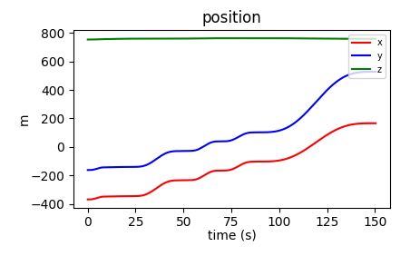
We ran our path-finding algorithm described in Section 6.1 with $(\Delta=1\ m,\ w=1.1)$ and obtained the trajectory shown in Table 4. Fig. 4 shows that the trajectory does indeed avoids all structures and terrain. We then used our bi-section algorithm with $\delta_{t}=0.05$ and $s_{max}=400\ rad/s$ to determine the minimum times required for each part of the mission which are shown in Table 4. Finally, we ran our controller with a simulation which provided the motor speeds presented in Fig. 5 and positions presented in Fig. 6.

8 Conclusion

We studied the problem of payload transportation by a single quadcopter in urban areas by considering the combined system of quadcopter and payload together as a rigid body. We used USGS LIDAR data to generate an elevation map for the University of Arizona. We then applied a hybrid approach, integrating a high-level motion planner with a low-level trajectory control, to safely plan a payload transportation mission assuring collision avoidance and boundedness of rotor angular speeds and trajectory tracking. In particular, the high-level motion planner combines the A* search with polynomial planning to obtain a collision-free desired trajectory minimizing travel distance from the initial position to the target destination. We showed that the quadcopter can stably track the desired trajectory by applying the input-output feedback linearization control.

Acknowledgments

This work has been supported by the National Science Foundation under Award Nos. 2133690 and 1914581.

References

Puri [2005] Puri, A., “A survey of unmanned aerial vehicles (UAV) for traffic surveillance,” Department of computer science and engineering, University of South Florida, 2005, pp. 1–29.
Kanistras et al. [2013] Kanistras, K., Martins, G., Rutherford, M. J., and Valavanis, K. P., “A survey of unmanned aerial vehicles (UAVs) for traffic monitoring,” 2013 International Conference on Unmanned Aircraft Systems (ICUAS), IEEE, 2013, pp. 221–234.
Surmann et al. [2019] Surmann, H., Worst, R., Buschmann, T., Leinweber, A., Schmitz, A., Senkowski, G., and Goddemeier, N., “Integration of uavs in urban search and rescue missions,” 2019 IEEE International Symposium on Safety, Security, and Rescue Robotics (SSRR), IEEE, 2019, pp. 203–209.
Półka et al. [2017] Półka, M., Ptak, S., and Kuziora, Ł., “The use of UAV’s for search and rescue operations,” Procedia engineering, Vol. 192, 2017, pp. 748–752.
Tomic et al. [2012] Tomic, T., Schmid, K., Lutz, P., Domel, A., Kassecker, M., Mair, E., Grixa, I. L., Ruess, F., Suppa, M., and Burschka, D., “Toward a fully autonomous UAV: Research platform for indoor and outdoor urban search and rescue,” IEEE robotics & automation magazine, Vol. 19, No. 3, 2012, pp. 46–56.
Witczuk et al. [2018] Witczuk, J., Pagacz, S., Zmarz, A., and Cypel, M., “Exploring the feasibility of unmanned aerial vehicles and thermal imaging for ungulate surveys in forests-preliminary results,” International Journal of Remote Sensing, Vol. 39, No. 15-16, 2018, pp. 5504–5521.
Mathew et al. [2015] Mathew, N., Smith, S. L., and Waslander, S. L., “Planning paths for package delivery in heterogeneous multirobot teams,” IEEE Transactions on Automation Science and Engineering, Vol. 12, No. 4, 2015, pp. 1298–1308.
Arbanas et al. [2016] Arbanas, B., Ivanovic, A., Car, M., Haus, T., Orsag, M., Petrovic, T., and Bogdan, S., “Aerial-ground robotic system for autonomous delivery tasks,” 2016 IEEE international conference on robotics and automation (ICRA), IEEE, 2016, pp. 5463–5468.
Cicolani et al. [1995] Cicolani, L. S., Kanning, G., and Synnestvedt, R., “Simulation of the dynamics of helicopter slung load systems,” Journal of the American Helicopter Society, Vol. 40, No. 4, 1995, pp. 44–61.
Bernard and Kondak [2009] Bernard, M., and Kondak, K., “Generic slung load transportation system using small size helicopters,” 2009 IEEE International Conference on Robotics and Automation, IEEE, 2009, pp. 3258–3264.
Pounds et al. [2012] Pounds, P. E., Bersak, D. R., and Dollar, A. M., “Stability of small-scale UAV helicopters and quadrotors with added payload mass under PID control,” Autonomous Robots, Vol. 33, No. 1, 2012, pp. 129–142.
Oh et al. [2006] Oh, S.-R., Ryu, J.-C., and Agrawal, S. K., “Dynamics and control of a helicopter carrying a payload using a cable-suspended robot,” 2006.
Palunko et al. [2012] Palunko, I., Cruz, P., and Fierro, R., “Agile load transportation: Safe and efficient load manipulation with aerial robots,” IEEE robotics & automation magazine, Vol. 19, No. 3, 2012, pp. 69–79.
Michael et al. [2011] Michael, N., Fink, J., and Kumar, V., “Cooperative manipulation and transportation with aerial robots,” Autonomous Robots, Vol. 30, No. 1, 2011, pp. 73–86.
Maza et al. [2009] Maza, I., Kondak, K., Bernard, M., and Ollero, A., “Multi-UAV cooperation and control for load transportation and deployment,” Selected papers from the 2nd International Symposium on UAVs, Reno, Nevada, USA June 8–10, 2009, Springer, 2009, pp. 417–449.
Mellinger et al. [2013] Mellinger, D., Shomin, M., Michael, N., and Kumar, V., “Cooperative grasping and transport using multiple quadrotors,” Distributed autonomous robotic systems, Springer, 2013, pp. 545–558.
Rastgoftar and Atkins [2018] Rastgoftar, H., and Atkins, E. M., “Cooperative aerial lift and manipulation (calm),” Aerospace Science and Technology, Vol. 82, 2018, pp. 105–118.
Acosta et al. [2020] Acosta, J., De Cos, C., and Ollero, A., “Accurate control of Aerial Manipulators outdoors. A reliable and self-coordinated nonlinear approach,” Aerospace Science and Technology, Vol. 99, 2020, p. 105731.
Tang and Kumar [2015] Tang, S., and Kumar, V., “Mixed integer quadratic program trajectory generation for a quadrotor with a cable-suspended payload,” 2015 IEEE international conference on robotics and automation (ICRA), IEEE, 2015, pp. 2216–2222.
Yang and Xian [2019] Yang, S., and Xian, B., “Energy-based nonlinear adaptive control design for the quadrotor UAV system with a suspended payload,” IEEE Transactions on Industrial Electronics, Vol. 67, No. 3, 2019, pp. 2054–2064.
Sreenath et al. [2013a] Sreenath, K., Michael, N., and Kumar, V., “Trajectory generation and control of a quadrotor with a cable-suspended load-a differentially-flat hybrid system,” 2013 IEEE International Conference on Robotics and Automation, IEEE, 2013a, pp. 4888–4895.
Kim et al. [2013] Kim, S., Choi, S., and Kim, H. J., “Aerial manipulation using a quadrotor with a two dof robotic arm,” 2013 IEEE/RSJ International Conference on Intelligent Robots and Systems, IEEE, 2013, pp. 4990–4995.
Guerrero et al. [2015] Guerrero, M. E., Mercado, D., Lozano, R., and García, C., “Passivity based control for a quadrotor UAV transporting a cable-suspended payload with minimum swing,” 2015 54th IEEE Conference on Decision and Control (CDC), IEEE, 2015, pp. 6718–6723.
Guo et al. [2017] Guo, M., Su, Y., and Gu, D., “Mixed H2/H $\infty$ Tracking Control with Constraints for Single Quadcopter Carrying a Cable-suspended Payload,” IFAC-PapersOnLine, Vol. 50, No. 1, 2017, pp. 4869–4874.
Goodarzi [2016] Goodarzi, F. A., “Autonomous aerial payload delivery with quadrotor using varying length cable,” 2016 International Conference on Advanced Mechatronic Systems (ICAMechS), IEEE, 2016, pp. 394–399.
Sreenath et al. [2013b] Sreenath, K., Lee, T., and Kumar, V., “Geometric control and differential flatness of a quadrotor UAV with a cable-suspended load,” 52nd IEEE Conference on Decision and Control, IEEE, 2013b, pp. 2269–2274.
Goodarzi et al. [2014] Goodarzi, F. A., Lee, D., and Lee, T., “Geometric stabilization of a quadrotor UAV with a payload connected by flexible cable,” 2014 American Control Conference, IEEE, 2014, pp. 4925–4930.
Barawkar et al. [2017] Barawkar, S., Radmanesh, M., Kumar, M., and Cohen, K., “Admittance based force control for collaborative transportation of a common payload using two uavs,” Dynamic Systems and Control Conference, Vol. 58295, American Society of Mechanical Engineers, 2017, p. V003T39A007.
Mellinger et al. [2011] Mellinger, D., Lindsey, Q., Shomin, M., and Kumar, V., “Design, modeling, estimation and control for aerial grasping and manipulation,” 2011 IEEE/RSJ International Conference on Intelligent Robots and Systems, IEEE, 2011, pp. 2668–2673.
Michael et al. [2009] Michael, N., Kim, S., Fink, J., and Kumar, V., “Kinematics and statics of cooperative multi-robot aerial manipulation with cables,” International Design Engineering Technical Conferences and Computers and Information in Engineering Conference, Vol. 49040, 2009, pp. 83–91.
Sreenath and Kumar [2013] Sreenath, K., and Kumar, V., “Dynamics, control and planning for cooperative manipulation of payloads suspended by cables from multiple quadrotor robots,” rn, Vol. 1, No. r2, 2013, p. r3.
Rastgoftar and Kolmanovsky [2021] Rastgoftar, H., and Kolmanovsky, I. V., “Safe affine transformation-based guidance of a large-scale multiquadcopter system,” IEEE Transactions on Control of Network Systems, Vol. 8, No. 2, 2021, pp. 640–653.
Rastgoftar et al. [2021] Rastgoftar, H., Atkins, E. M., and Kolmanovsky, I. V., “Scalable Vehicle Team Continuum Deformation Coordination with Eigen Decomposition,” IEEE Transactions on Automatic Control, 2021.
Romano et al. [2019] Romano, M., Kuevor, P., Lukacs, D., Marshall, O., Stevens, M., Rastgoftar, H., Cutler, J., and Atkins, E., “Experimental evaluation of continuum deformation with a five quadrotor team,” 2019 American Control Conference (ACC), IEEE, 2019, pp. 2023–2029.