Phase transitions and thermodynamic geometry of a Kerr-Newman black hole in a cavityPreprint: CTP-SCU/2022011

How to define the quasi-local energy of a gravitational field in a spatially bounded cavity is an important topic in general relativity. For example, developing a tool to calculate the quasi-local energy could help us better understand the theory of gravitation itself. Moreover, correct thermodynamic quantities of black holes are probably at the quasi-local level. For the simplest non-trivial black hole solution in general relativity, the Schwarzschild black hole, whose thermodynamics in a cavity was first investigated with the help of the Euclidean action York:1986it, where a phase transition that occurs between thermal flat spacetime and the black hole was found to be very similar to that of the Hawking-Page in AdS space Hawking:1982dh. The thermodynamic quantities are consistent with the results from the later proposed Brown-York definition of quasi-local quantities Brown:1992br. By means of such a definition, thermodynamic quantities for some simple gravitational systems enclosed by a cavity were obtained Brown:1994gs. Afterwards, the thermodynamics and phase transitions of a RN black hole in a cavity were studied in a grand canonical ensemble Braden:1990hw and a canonical ensemble Carlip:2003ne; Lundgren:2006kt, which also exhibit some similarities to the black hole in asymptotic AdS space.

Recently, some works have been focusing on thermodynamics of various black holes in a cavity, which devoted to comparing phase transitions of black holes under different boundary conditions Wang:2019kxp; Liang:2019dni; Wang:2019urm; Huang:2021iyf; Yao:2021zid; Huang:2021eby, i.e., AdS space and the cavity. A main conclusion is that the thermodynamics and phase transitions of black holes under the two different boundary conditions show close resemblances but several dissimilarities in details. Furthermore, the thermodynamics of a black hole in a cavity was discussed in an extended phase space, where volume of the cavity was treated as thermodynamic volume Wang:2020hjw. On the whole, most discussions about the thermodynamics of black holes in a cavity especially phase transitions, were based on static black holes. Although a rotating BTZ black hole was studied in Huang:2021eby, it did not show rich phase structures due to its non-negative heat capacity. Therefore, one naturally generalizes the study to a four-dimensional black hole with an angular momentum.

On the other hand, although black holes can undergo phase transitions, an complete quantum gravity theory that can explain them microscopically still remains absent. Nonetheless, there are many attempts trying to give microscopic interpretations of black hole thermodynamics. The thermodynamic geometry method, which sheds some fresh insights into equilibrium thermodynamics, has been proved to be a useful tool to probe microscopic structures of black holes. The idea of using the Riemannian geometry to study equilibrium thermodynamics was proposed by Weinhold 1975JChPh..63.2479W, who introduced a curvature scalar of a metric defined by the derivative of the internal energy with respect to the entropy and other extensive variables. Since this geometry seems meaningless in physics, Ruppeiner further developed the theory and introduced a new metric, but defined by the derivative of the entropy with respect to other extensive variables Ruppeiner:1995zz. In this definition, the line element measures the distance between two neighboring fluctuation states in equilibrium thermodynamic. The Riemann curvature scalar based on this metric is also called the Ruppeiner invariant. After computing the Ruppeiner invariant in various thermodynamic systems, such as ideal gas PhysRevA.20.1608; PhysRevA.41.2200, ideal paramagnet PhysRevA.39.6515, ideal quantum gas 1990JPhA…23..467J, one-dimensional Ising model PhysRevA.24.488, and so forth, one came to an empirical conclusion that the positive/negative curvature scalar is caused by the repulsive/attractive interaction. This intriguing phenomenon was then generalized to the study of thermodynamics of black holes Ferrara:1997tw. In the twenty years thereafter applications of the thermodynamic geometry in black holes attracted many theoretical interests Cai:1998ep; Aman:2003ug; Shen:2005nu; Aman:2005xk; Sarkar:2006tg; Quevedo:2008xn; Ruppeiner:2008kd; Banerjee:2010bx; Banerjee:2010da; Niu:2011tb; Zhang:2015ova; Wei:2015iwa; Wei:2019yvs; Wei:2019uqg; Wei:2020poh; Wei:2021lmo. Nonetheless, the thermodynamic geometry of black holes in a cavity did not receive much attentions, which might help us to probe microstructures of black holes in a new boundary condition. Although some researches have made initial progress by comparing it in AdS space and a cavity Wang:2019cax; Wang:2021llu, we point out that these studies are somewhat incomplete since they only considered the simply case of a RN black hole.

To deepen our understanding of microstructures of black holes in a cavity, we calculate the Ruppeiner invariant of a general black hole, i.e., a Kerr-Newman black hole. The Kerr-Newman metric is an exact solution of the Einstein-Maxwell equation, which describes stationary spacetime with an angular momentum and an electric charge Newman:1965my. Later on, with the advent of the AdS/CFT conjecture Maldacena:1997re; Witten:1998qj, the thermodynamics of a Kerr-Newman black hole in AdS space was studied in Caldarelli:1999xj, where the Hawking-Page phase transition was found in a grand canonical ensemble, and a van de Waals-like phase transition was found in a canonical ensemble. Other thermodynamic properties of the Kerr-Newman black hole under different conditions were extensively studied Davies:1989ey; Sahay:2010wi; Cembranos:2011sr; Cheng:2016bpx; Biro:2019rms; Garcia-Compean:2020gii. It was proposed by Smarr that under some specific conditions, a two-dimensional hypersurface of the Kerr spacetime can not be globally embedded in the three-dimensional Euclidean space Smarr:1973zz, therefore only the quasi-local energy with a small angular momentum of the Kerr black hole was obtained Martinez:1994ja. A counterterm prescription inspired by the AdS/CFT conjecture was proposed Kraus:1999di; Mann:1999pc; Balasubramanian:1999re; Lau:1999dp, which solved this issue and was used to calculate the quasi-local energy and thermodynamic quantities of various rotating black holes Dehghani:2001af; Dehghani:2002np; Dehghani:2002nt.

In this work, we investigate the phase transitions and thermodynamic geometry of a Kerr-Newman black hole in a cavity as well as two reduced cases, i.e., a RN black hole in a cavity and a Kerr black hole in a cavity. The quasi-local energy we adopt is defined by the Brown-York method. To make the Hamiltonian well defined, a counterterm prescription is considered. The following part of this paper is organized as follows: We first derive the quasi-local energy for a Kerr-Newman black hole and construct the first law of thermodynamics in section II. In section III, we study the phase transition in a canonical ensemble based on the quantities defined in the last section. Two reduced cases are also discussed. In section IV, we probe the microscopic interactions of the black holes with the help of the thermodynamic geometry. The closing remarks are presented in section V.

We start from the volume gravitational action coupled to the electromagnetic field,

$$\mathcal{S}_{v}=\frac{1}{16\pi}\int_{\mathcal{M}}d^{4}x\sqrt{-g}\left(R-F^{\mu\nu}F_{\mu\nu}\right),$$

(1)

where $R$ is the Ricci scalar of the manifold $\mathcal{M}$, and $F_{\mu\nu}=\partial_{\mu}A_{\nu}-\partial_{\nu}A_{\mu}$ is the electromagnetic field tensor. To give the correct field equation, a boundary term is required, and it is given by

$$\mathcal{S}_{b}=\frac{1}{8\pi}\int_{\partial\mathcal{M}}d^{3}x\varepsilon\sqrt{|h|}K.$$

(2)

The integral of the above formula is calculated on the boundary $\partial\mathcal{M}$, which can be written as a union of three parts $\partial\mathcal{M}=(-\Sigma_{t^{{}^{\prime}}})\cup\Sigma_{t^{{}^{\prime\prime}}}\cup\mathscr{B}$, where $\Sigma_{t^{{}^{\prime}}}$, $\Sigma_{t^{{}^{\prime\prime}}}$ are two spacelike boundaries, and $\mathscr{B}$ is a timelike boundary. Besides, $K$ is the trace of the extrinsic curvature on $\partial\mathcal{M}$ as embedded in $\mathcal{M}$, and $\varepsilon=1$ if $\partial\mathcal{M}$ is timelike while $\varepsilon=-1$ if $\partial\mathcal{M}$ is spacelike. The foliation of the manifold is presented in FIG. 1. It turns out that the value of the action is divergent if one extends the boundary to infinity. Therefore, an extra term is needed to eliminate this divergence. Although this term is not always uniquely determined Chan:1996sx, a natural choice is

$$\mathcal{S}_{0}=-\frac{1}{8\pi}\int_{\partial\mathcal{M}}d^{3}x\varepsilon\sqrt{|h|}K_{0},$$

(3)

where $K_{0}$ is the extrinsic curvature of $\partial\mathcal{M}$ that embedded in flat spacetime. This term makes the value of the action vanish when spacetime is flat. For a Kerr spacetime, not all the two-boundary surfaces are possible to be globally embedded in three-dimensional Euclidean space Smarr:1973zz, which makes the extra term not well defined, and hence only the quasi-local energy with a small angular momentum is obtained Martinez:1994ja. To address these difficulties, one can resort to a counterterm prescription, which suggests that the term $\mathcal{S}_{0}$ in Eq. (3) should be replaced by Kraus:1999di; Mann:1999pc; Balasubramanian:1999re

$$\mathcal{S}_{ct}=-\frac{1}{8\pi}\int_{\partial\mathcal{M}}d^{3}x\varepsilon\sqrt{|h|}\sqrt{2\mathscr{R}},$$

(4)

where $\mathscr{R}$ denotes the Ricci scalar on the three-boundary $\mathscr{B}$. Some analyses focus on another similar counterterm that substitutes $\mathscr{R}$ with the Ricci scalar of the two-boundary $\mathcal{B}$, which is also called a lightcone reference Lau:1999dp. In the following part, we will calculate thermodynamic quantities based on the counterterm in Eq. (4). Geometric quantities in this paper are shown in TABLE 1.

To obtain the Hamiltonian from the action, one performs a (3 + 1) decomposition on the manifold $\mathcal{M}$ and arrives at poisson2004relativist

$\displaystyle\mathcal{S}=\frac{1}{16\pi}\int_{t^{{}^{\prime}}}^{t^{{}^{\prime\prime}}}dt\left[\int_{\Sigma_{t}}d^{3}x\left(\mathcal{R}+K^{ab}K_{ab}-K^{2}-F^{\mu\nu}F_{\mu\nu}\right)N\sqrt{h}+2\int_{\mathcal{B}}d^{2}x\left(k-\sqrt{2\mathscr{R}}\right)N\sqrt{\sigma}\right],$

(5)

where $\Sigma_{t}$ describes a constant time hypersurface, $\mathcal{R}$ is the Ricci scalar on $\Sigma_{t}$, $N$ is the lapse function, $\sigma$ denotes the determinant of the metric of $\mathcal{B}$, and $k$ is the trace of the extrinsic curvature of $\mathcal{B}$ as embedded in $\Sigma_{t}$. Regarding $h_{ab}$ as the dynamic variable of the gravitational field, one obtains the corresponding conjugated momentum

$$p^{ab}=\frac{\partial\left(\sqrt{-g}\mathcal{L}_{G}\right)}{\partial\dot{h}_{ab}}=\frac{1}{16\pi}\sqrt{h}(K^{ab}-Kh^{ab}),$$

(6)

where $\mathcal{L}_{G}$ is the Lagrangian of the pure gravitational field. The dot over $h_{ab}$ denotes the Lie derivative along $t^{\alpha}=Nn^{\alpha}+N^{a}e^{\alpha}_{a}$, where $N^{a}$ is the shift function. The dynamic variable of the pure electromagnetic field is $\partial_{0}A_{a}$, and hence the conjugated momentum is

$$\mathcal{P}^{a}=-\frac{\sqrt{-g}}{16\pi}\frac{\partial\left(F^{\mu\nu}F_{\mu\nu}\right)}{\partial\left(\partial_{0}A_{a}\right)}=-\frac{\sqrt{-g}}{4\pi}F^{0a}.$$

(7)

Consequently, the Hamiltonian density can be written as

$$\mathcal{H}=p^{ab}\dot{h}_{ab}+\mathcal{P}^{a}\partial_{0}A_{a}-\sqrt{-g}\left(\mathcal{L}_{G}-F^{\mu\nu}F_{\mu\nu}\right).$$

(8)

Integrating the Hamiltonian density in the space region $\Sigma_{t}$ and adding the boundary term, we obtain the Hamiltonian of the system,

	$\displaystyle H$	$\displaystyle=\frac{1}{16\pi}\int_{\Sigma_{t}}d^{3}x\sqrt{h}\left(N\mathcal{C}-2N_{a}\mathcal{C}^{a}+A_{0}\mathcal{G}\right)$		(9)
		$\displaystyle-\frac{1}{8\pi}\int_{\mathcal{B}}d^{2}x\sqrt{\sigma}\left[N\left(k-\sqrt{2\mathscr{R}}\right)-N_{a}\left(K^{ab}-Kh^{ab}\right)r_{b}-\frac{8\pi}{\sqrt{h}}A_{0}r_{a}\mathcal{P}^{a}\right],$

where $r_{a}$ is the unit normal of $\mathcal{B}$ as embedded in $\Sigma_{t}$. Furthermore, we have two constraint equations from general relativity and one from electromagnetism. The Hamiltonian constraint reads

$$\mathcal{C}=K^{ab}K_{ab}-K^{2}-\mathcal{R}+16\pi\rho=0,$$

(10)

where $\rho=T_{\alpha\beta}n^{\alpha}n^{\beta}$ is the energy density of the electromagnetic field, and $T_{\alpha\beta}$ denotes the energy-momentum tensor,

$$T^{\alpha\beta}=\frac{1}{4\pi}g_{\mu\nu}F^{\alpha\mu}F^{\beta\nu}-\frac{1}{16\pi}g^{\alpha\beta}F^{\mu\nu}F_{\mu\nu}.$$

(11)

The momentum constraint reads

$$\mathcal{C}^{a}=\left(K^{ab}-Kh^{ab}\right)_{|b}-8\pi j^{a}=0,$$

(12)

where $j_{a}=T_{\alpha\beta}e^{\alpha}_{a}n^{\beta}$ is the momentum density of the field. The Gauss’s-law constraint reads

$$\mathcal{G}=-\frac{16\pi}{\sqrt{h}}\mathcal{P}^{a}{}_{,a}=0.$$

(13)

With these constraint equations, the Hamiltonian reduces to

$$H=-\frac{1}{8\pi}\int_{\mathcal{B}}d^{2}x\sqrt{\sigma}\left[N\left(k-\sqrt{2\mathscr{R}}\right)-N_{a}\left(K^{ab}-Kh^{ab}\right)r_{b}-\frac{8\pi}{\sqrt{h}}A_{0}r_{a}\mathcal{P}^{a}\right].$$

(14)

The mass-energy of the gravitational system inside the boundary $\mathcal{B}$ is defined as the first term in the Hamiltonian (14) with the choice of lapse $N=1$ Brown:1992br; Szabados:2004xxa,

$\displaystyle E$

$\displaystyle=-\frac{1}{8\pi}\int_{\mathcal{B}}d^{2}x\sqrt{\sigma}\left(k-\sqrt{2\mathscr{R}}\right),$

(15)

which will be regarded as the internal energy of the thermodynamic system.

We consider the Kerr-Newman spacetime, whose metric in the Boyer-Lindquist-type coordinates is given by Newman:1965my; poisson2004relativist

	$\displaystyle ds^{2}=-\frac{\Delta}{\rho^{2}}\left(dt-a\sin^{2}{\theta}d\phi\right)^{2}+$	$\displaystyle\frac{\rho^{2}}{\Delta}dr^{2}+\rho^{2}d\theta^{2}+\frac{\sin^{2}{\theta}}{\rho^{2}}\Big[adt-\left(r^{2}+a^{2}\right)d\phi\Big]^{2},$		(16)
	$\displaystyle A_{\alpha}dx^{\alpha}$	$\displaystyle=-\frac{Qr}{\rho^{2}}\left(dt-a\sin^{2}{\theta}d\phi\right),$

with

	$\displaystyle\rho^{2}$	$\displaystyle=r^{2}+a^{2}\cos^{2}{\theta},$		(17)
	$\displaystyle\Delta$	$\displaystyle=r^{2}-2Mr+a^{2}+Q^{2},$

where $M$ is the ADM mass, $a=J/M$ is the magnitude of the angular momentum per unit mass, and $Q$ is the charge. The event horizon radius $r_{+}$ is determined by a coordinate singularity $\Delta=0$, i.e., $r_{+}^{2}-2Mr_{+}+a^{2}+Q^{2}=0$. The induced line element on the constant time hypersurface $\Sigma_{t}$ can be written as

$$ds^{2}|_{\Sigma_{t}}=\frac{\rho^{2}}{\Delta}dr^{2}+\rho^{2}d\theta^{2}+\frac{\sin^{2}{\theta}}{\rho^{2}}\left[\left(r^{2}+a^{2}\right)^{2}-a^{2}\Delta\sin^{2}{\theta}\right]d\phi^{2}.$$

(18)

We consider that the black hole is enclosed by a cavity with a fixed radius $r_{B}$. The line element on the hypersurface $\mathcal{B}$, which is the wall of the cavity thus is given by

$\displaystyle ds^{2}|_{\mathcal{B}}=\left(r_{B}^{2}+a^{2}\cos^{2}{\theta}\right)d\theta^{2}+\frac{\sin^{2}{\theta}}{r_{B}^{2}+a^{2}\cos^{2}{\theta}}\left[\left(r_{B}^{2}+a^{2}\right)^{2}-a^{2}\left(r_{B}^{2}-2Mr_{B}+a^{2}+Q^{2}\right)\sin^{2}{\theta}\right]d\phi^{2}.$

(19)

The determinant of the metric of $\mathcal{B}$ can be extracted from the line element above,

$$\sigma=a^{4}\sin^{2}{\theta}\cos^{2}{\theta}+2a^{2}mr_{B}\sin^{4}{\theta}-a^{2}Q^{2}\sin^{4}{\theta}-a^{2}r_{B}^{2}\sin^{4}{\theta}+2a^{2}r_{B}^{2}\sin^{2}{\theta}+r_{B}^{4}\sin^{2}{\theta}.$$

(20)

The trace of the extrinsic curvature $k_{ab}$ of $\mathcal{B}$ that embedded in $\Sigma_{t}$ is

$$k=r^{a}{}_{|a}=\frac{a^{2}\sin^{2}{\theta}\left(r_{B}-M\right)-2r_{B}\left(a^{2}+r_{B}^{2}\right)}{a^{2}\sin^{2}{\theta}\left(a^{2}-2Mr_{B}+Q^{2}+r_{B}^{2}\right)-\left(a^{2}+r_{B}^{2}\right)^{2}}\times\left(\frac{a^{2}-2Mr_{B}+Q^{2}+r_{B}^{2}}{a^{2}\cos^{2}{\theta}+r_{B}^{2}}\right)^{1/2}.$$

(21)

The Ricci scalar of the boundary $\mathscr{B}$ with a fixed radius arrives at

$$\mathscr{R}=\frac{2r_{B}^{4}+2a^{2}\left(r_{B}^{2}-2Mr_{B}+Q^{2}\right)\cos^{2}{\theta}}{\left(r_{B}^{2}+a^{2}\cos^{2}{\theta}\right)^{3}}.$$

(22)

With these preliminaries, we then calculate the energy of the black hole in a cavity. A straightforward calculation of Eq. (15) gives

$\displaystyle E$

$\displaystyle=\int_{0}^{\pi}d\theta\text{ }E_{\theta}\left(a,M,r_{B},Q,\theta\right),$

(23)

where

	$\displaystyle E_{\theta}$	$\displaystyle\left(a,M,r_{B},Q,\theta\right)=\left[\left(a^{2}+r_{B}^{2}\right)^{2}\sin^{2}{\theta}-a^{2}\sin^{4}{\theta}\left(a^{2}-2Mr_{B}+Q^{2}+r_{B}^{2}\right)\right]^{1/2}$		(24)
		$\displaystyle\times\left\{\frac{2a^{2}\cos^{2}{\theta}\left(r_{B}^{2}+Q^{2}-2Mr_{B}\right)+2r_{B}^{4}}{\left(2a^{2}\cos^{2}{\theta}+2r_{B}^{2}\right)^{3}}\right\}^{1/2}$
		$\displaystyle+\frac{a^{2}\sin^{4}{\theta}(r_{B}-M)-2r_{B}\left(a^{2}+r_{B}^{2}\right)\sin^{2}{\theta}}{4\left[\left(a^{2}+r_{B}^{2}\right)^{2}\sin^{2}{\theta}-a^{2}\sin^{4}{\theta}\left(a^{2}-2Mr_{B}+Q^{2}+r_{B}^{2}\right)\right]^{1/2}}\times\left(\frac{a^{2}-2Mr_{B}+Q^{2}+r_{B}^{2}}{a^{2}\cos^{2}{\theta}+r_{B}^{2}}\right)^{1/2}.$

Moreover, extending the cavity radius to infinity, we find that the result is consistent with the ADM mass,

$$\lim_{r_{B}\to\infty}E=M.$$

(25)

The entropy of the Kerr-Newman black hole equals to one quarter of the event horizon area,

$$S=\frac{1}{4}A=\pi\left(r_{+}^{2}+a^{2}\right).$$

(26)

We consider the following three equations: the event horizon determined by $\Delta=0$ in Eq. (17), the angular momentum $J=Ma$ and the entropy in Eq. (26). Solving these equations, one obtains the rotating parameter $a$ and the ADM mass $M$ as functions of the entropy, the angular momentum and the charge: $a(S,J,Q)$ and $M(S,J,Q)$. After inserting functions $a(S,J,Q)$ and $M(S,J,Q)$ into $E(a,M,r_{B},Q)$ in Eq. (23), we rewrite the energy as $E\left(S,J,Q,r_{B}\right)$. We then define the temperature as the derivative of the energy with respect to the entropy while keeping $J$, $Q$, $r_{B}$ fixed,

$$T\left(S,J,Q,r_{B}\right)=\left(\frac{\partial E}{\partial S}\right)_{J,Q,r_{B}}=\int_{0}^{\pi}d\theta\left(\frac{\partial E_{\theta}}{\partial S}\right)_{J,Q,r_{B}}.$$

(27)

In the second equality, we have swapped the order of the derivative and the integral. Similarly, the angular velocity and the electric potential are defined as

	$\displaystyle\Omega(S,J,Q,r_{B})$	$\displaystyle=\int_{0}^{\pi}d\theta\left(\frac{\partial E_{\theta}}{\partial J}\right)_{S,Q,r_{B}},$		(28)
	$\displaystyle\Phi(S,J,Q,r_{B})$	$\displaystyle=\int_{0}^{\pi}d\theta\left(\frac{\partial E_{\theta}}{\partial Q}\right)_{S,J,r_{B}}.$

Therefore, the first law of thermodynamics can be written as

$$dE=TdS+\Omega dJ+\Phi dQ.$$

(29)

Without loss of generality, we set the cavity radius $r_{B}=1$ and keep it invariant in the following discussions to simplify the calculation.

We first analyze thermodynamic stability of the black hole in a canonical ensemble by considering the heat capacity at fixed angular momentum and the charge,

$$C_{J,Q}=\lim_{\Delta T\to 0}\left(\frac{\Delta Q_{t}}{\Delta T}\right)_{J,Q}=T\left(\frac{\partial S}{\partial T}\right)_{J,Q}=T\bigg/\left(\frac{\partial T}{\partial S}\right)_{J,Q},$$

(30)

where $\Delta Q_{t}$ refers to the heat absorbed by the black hole. The sign of the heat capacity agrees with the sign of the derivative of the temperature with respect to the entropy, and so we turn to consider this term. Due to the absence of an analytic expression, we resort to numerical methods to investigate the heat capacity. We find there are three patterns for the temperature as a function of the entropy, corresponding to three regions in the $J$-$Q$ plane, as shown in FIG. 2.

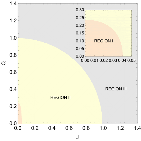
In Region I, the curve of the temperature with respect to the entropy can be divided into three branches, dubbed as small black hole, medium black hole and large black hole, as shown in the upper left panel of FIG. 3. The thermodynamic stability based on the heat capacity can be read off from slopes of $T$-$S$ curves, i.e., the positive/negative slope corresponds to stable/unstable phase. Therefore, the small/medium/large black hole is thermodynamically stable/unstable/stable. In a canonical ensemble where the angular momentum $J$ and the charge $Q$ are fixed, the Helmholtz free energy, defined as $F=E-TS$ is used to investigate phase transitions. We first write the free energy as a function of $S$, $J$ and $Q$: $F(S,J,Q)$ and then plot it as a function of $T(S,J,Q)$ while regarding $S$ as the variable parameter in the lower left panel of FIG. 3. At a low temperature, there is only a small black hole, which is thermodynamically stable. As the temperature increases, a first-order phase transition occurs from the small black hole to the large black hole. After the phase transition, the small black hole becomes a metastable phase, and the large black hole becomes the most stable phase.

In Region II, there is only one branch in the $T$-$S$ curve, as shown in the upper right panel of FIG. 3. The branch has a positive slope, indicating a thermodynamically stable phase in this region, which is dubbed as single phase. The free energy against the temperature of the single phase is displayed in the lower right panel of FIG. 3, which shows that there is no phase transition in Region II. In Region III, there is no black hole solution, and thus it is a non-physical region.

In addition, we discuss two reduced cases, i.e., a RN black hole in a cavity and a Kerr black hole in a cavity. And we will show that these black holes have similar phase structures in a cavity. Thermodynamic quantities of a RN black hole in a cavity can be obtained from those of a Kerr-Newman by making the angular momentum vanishing,

	$\displaystyle E$	$\displaystyle=r_{B}-r_{B}\left(1+\frac{Q^{2}}{r_{B}^{2}}-\frac{\pi^{1/2}Q^{2}}{S^{1/2}r_{B}}-\frac{S^{1/2}}{\pi^{1/2}r_{B}}\right)^{1/2},$		(31)
	$\displaystyle T$	$\displaystyle=\frac{1}{4\pi^{1/2}S^{1/2}}\left(1-\frac{\pi Q^{2}}{S}\right)\left(1+\frac{Q^{2}}{r_{B}^{2}}-\frac{\pi^{1/2}Q^{2}}{S^{1/2}r_{B}}-\frac{S^{1/2}}{\pi^{1/2}r_{B}}\right)^{-1/2},$
	$\displaystyle\Phi$	$\displaystyle=\left(\frac{\pi^{1/2}Q}{S^{1/2}}-\frac{Q}{r_{B}}\right)\left(1+\frac{Q^{2}}{r_{B}^{2}}-\frac{\pi^{1/2}Q^{2}}{S^{1/2}r_{B}}-\frac{S^{1/2}}{\pi^{1/2}r_{B}}\right)^{-1/2},$
	$\displaystyle F$	$\displaystyle=r_{B}-r_{B}\left(1+\frac{Q^{2}}{r_{B}^{2}}-\frac{\pi^{1/2}Q^{2}}{S^{1/2}r_{B}}-\frac{S^{1/2}}{\pi^{1/2}r_{B}}\right)^{1/2}$
		$\displaystyle-\frac{S^{1/2}}{4\pi^{1/2}}\left(1-\frac{\pi Q^{2}}{S}\right)\left(1+\frac{Q^{2}}{r_{B}^{2}}-\frac{\pi^{1/2}Q^{2}}{S^{1/2}r_{B}}-\frac{S^{1/2}}{\pi^{1/2}r_{B}}\right)^{-1/2}.$

These results are consistent with previous studies Braden:1990hw; Wang:2020hjw. The free energy $F$ as functions of the temperature $T$ with fixed charges can show similar swallow tail behaviors as the one of a Kerr-Newman black hole in a cavity, as shown in upper panels of FIG. 4. When $Q<Q_{c}$, where $Q_{c}$ is the critical value of the charge, there are three different phases. The small black hole goes through a first-order phase transition and converts to the large black hole as $T$ increases. When $Q>Q_{c}$, there is only one single phase, and no phase transition occurs.

Similarly, thermodynamic quantities of a Kerr black hole in a cavity can be obtained by constraining the charge $Q=0$ from a Kerr-Newman black hole. These quantities are too complex to be presented here, but we have verified that they are also consistent with previous research Dehghani:2001af. The $F$-$T$ curves of the Kerr black hole in a cavity also show similar swallowtail behavior, as shown in lower panels of FIG. 4. When $J<J_{c}$, where $J_{c}$ is the critical value of the angular momentum, there are also three branches, corresponding three phases in the thermodynamic system. As $T$ increases, there is a small-to-large black hole phase transition. When $J>J_{c}$, there is only a single phase with no phase transition occurring.

In this section, we study microstructures of these black holes in a cavity with the help of the thermodynamic geometry method. Before discussing some concrete details, we first make a brief review on the thermodynamic geometry of a general thermodynamic system. The Ruppeiner metric is defined as Ruppeiner:1995zz

$$g^{R}_{\alpha\beta}=-\frac{\partial^{2}S}{\partial x^{\alpha}\partial x^{\beta}},$$

(32)

where $S$ is the entropy, and $x^{\alpha}=\left(U,V,...\right)$ are extensive variables. The first law of thermodynamics can be written as

$$dS=\frac{1}{T}dU+\frac{P}{T}dV.$$

(33)

According to the definition of the Ruppeiner metric, the line element is

$$ds^{2}=g_{\alpha\beta}^{R}dx^{\alpha}dx^{\beta}=\frac{1}{T}dTdS-\frac{1}{T}dPdV.$$

(34)

The line element can be simplified to a diagonal form by choosing $S$ and $P$ as independent thermodynamic coordinates,

	$\displaystyle ds^{2}$	$\displaystyle=\frac{1}{T}\left[\left(\frac{\partial T}{\partial S}\right)_{P}dS+\left(\frac{\partial T}{\partial P}\right)_{S}dP\right]dS-\frac{1}{T}dP\left[\left(\frac{\partial V}{\partial S}\right)_{P}dS+\left(\frac{\partial V}{\partial P}\right)_{S}dP\right]$		(35)
		$\displaystyle=\frac{1}{T}\left(\frac{\partial T}{\partial S}\right)_{P}dS^{2}-\frac{1}{T}\left(\frac{\partial V}{\partial P}\right)_{S}dP^{2},$

where off-diagonal terms are eliminated by the Maxwell relation $\left(\frac{\partial T}{\partial P}\right)_{S}=\left(\frac{\partial V}{\partial S}\right)_{P}$. Having known the thermodynamic coordinates and the metric, we can construct a curvature scalar by using the definition of the Riemannian geometry, which is called the Ruppeiner invariant. A general form of the Rupppeiner invariant then reads

$$R_{G}=\frac{T}{2\left(\frac{\partial T}{\partial S}\right)^{2}\left(\frac{\partial V}{\partial P}\right)}\left[\left(\frac{\partial^{2}T}{\partial P^{2}}\right)\left(\frac{\partial^{2}T}{\partial S^{2}}\right)-\left(\frac{\partial^{2}V}{\partial S^{2}}\right)^{2}\right]-\frac{T}{2\left(\frac{\partial T}{\partial S}\right)\left(\frac{\partial V}{\partial P}\right)^{2}}\left[\left(\frac{\partial^{2}V}{\partial S^{2}}\right)\left(\frac{\partial^{2}V}{\partial P^{2}}\right)-\left(\frac{\partial^{2}T}{\partial P^{2}}\right)^{2}\right],$$

(36)

which, apparently has been written as a function of $S$ and $P$, and this will be very helpful for our next discussions. Interestingly, the Ruppeiner invariant has an empirical conclusion: The positive/negative curvature scalar reflects the repulsive/attractive interaction of the microsystem, which implies that we can get some information about microscopic interactions of black holes by computing the Ruppeiner invariant. In the following part of this paper, we first discuss two simplified cases, that is, a RN black hole in a cavity and a Kerr black hole in a cavity. Although the thermodynamic geometry of the former case has been studied in Wang:2019cax, we think it deserves to review this result here and compare it with the Kerr and Kerr-Newman cases.

In this work, we mainly studied the thermodynamic, phase transition and the thermodynamic geometry of a Kerr-Newman black hole in a cavity as well as a RN black hole in a cavity and a Kerr black hole in a cavity, and made a comparison between them. In order to derive the quasi-local energy of a Kerr-Newman black hole in a cavity from the Hamiltonian, we resorted to a counterterm prescription, which had succeeded in defining the quasi-local energy of a Kerr spacetime in previous researches. According to the quasi-local energy, we derived thermodynamic quantities and constructed the first law of thermodynamics of the black hole.

Using the thermodynamic quantities defined above, we further analyzed the phase transition of the black hole in a cavity. It shows that there are three regions in the angular momentum-charge plane, as shown in FIG. 2. In Region I, the black hole will go through a first-order phase transition as the temperature increases. In Region II, there is a single phase that is globally thermodynamically stable, and no phase transition occurs. In Region III, there is no black hole solution, which means that it is a non-physical region. The $T$-$S$ and $F$-$T$ curves of the black hole in Region I and Region II are shown in FIG. 3. We concluded that the phase structure of a Kerr-Newman black hole in a cavity can show extensive similarities to the one in AdS spacetime.

The thermodynamic geometry is a helpful tool to probe microstructures of black holes. As a preparation, we first calculated the Ruppeiner invariant of a RN black hole and a Kerr black hole in a cavity. Our results show that, microstructures of the charged black hole and the rotating black hole show great differences. For a RN black hole, the microscopic interaction is dominated by an attractive interaction in the small black hole phase and the large black phase. In the single phase region, the type of the dominating interaction is determined by concrete values of the charge and the temperature, as shown in the left panel of FIG. 7. For a Kerr black hole, attractive and repulsive interactions can both exist in these three phases. When the black hole is both rotating and charged, we choosed different thermodynamic variables $x^{\alpha}$ to investigate its microstructures in different ensembles. Phase diagrams with fixed angular momentum $J$ and fixed charge $Q$ are both exhibited in FIG. 8. The microstructure of a Kerr-Newman black hole in a cavity depends on thermodynamic variables $x^{\alpha}$ that we choose. When we choose $x^{\alpha}=(U,\Phi)$, the black hole exhibits microscopic interactions that are somewhat more similar to a RN black hole, and when we choose $x^{\alpha}=(U,\Omega)$, the black hole exhibits microscopic interactions more similar to a Kerr black hole. These results indicate that microstructures of black holes in a cavity are very sensitive to the selection of thermodynamic variables and their states.

We are grateful to Yihe Cao, Qi Xu and Jiayi Wu for useful discussions and valuable comments. This work is supported by NSFC (Grant No.12147207 and 12105031).

References

- (1) James W. York, Jr. Black hole thermodynamics and the Euclidean Einstein action. Phys. Rev. D, 33:2092–2099, 1986. doi:10.1103/PhysRevD.33.2092.
- (2) S. W. Hawking and Don N. Page. Thermodynamics of Black Holes in anti-De Sitter Space. Commun. Math. Phys., 87:577, 1983. doi:10.1007/BF01208266.
- (3) J. David Brown and James W. York, Jr. Quasilocal energy and conserved charges derived from the gravitational action. Phys. Rev. D, 47:1407–1419, 1993. arXiv:gr-qc/9209012, doi:10.1103/PhysRevD.47.1407.
- (4) J. David Brown, J. Creighton, and Robert B. Mann. Temperature, energy and heat capacity of asymptotically anti-de Sitter black holes. Phys. Rev. D, 50:6394–6403, 1994. arXiv:gr-qc/9405007, doi:10.1103/PhysRevD.50.6394.
- (5) Harry W. Braden, J. David Brown, Bernard F. Whiting, and James W. York, Jr. Charged black hole in a grand canonical ensemble. Phys. Rev. D, 42:3376–3385, 1990. doi:10.1103/PhysRevD.42.3376.
- (6) Steven Carlip and S. Vaidya. Phase transitions and critical behavior for charged black holes. Class. Quant. Grav., 20:3827–3838, 2003. arXiv:gr-qc/0306054, doi:10.1088/0264-9381/20/16/319.
- (7) Andrew P. Lundgren. Charged black hole in a canonical ensemble. Phys. Rev. D, 77:044014, 2008. arXiv:gr-qc/0612119, doi:10.1103/PhysRevD.77.044014.
- (8) Peng Wang, Houwen Wu, and Haitang Yang. Thermodynamics and Phase Transition of a Nonlinear Electrodynamics Black Hole in a Cavity. JHEP, 07:002, 2019. arXiv:1901.06216, doi:10.1007/JHEP07(2019)002.
- (9) Kangkai Liang, Peng Wang, Houwen Wu, and Mingtao Yang. Phase structures and transitions of Born–Infeld black holes in a grand canonical ensemble. Eur. Phys. J. C, 80(3):187, 2020. arXiv:1907.00799, doi:10.1140/epjc/s10052-020-7750-z.
- (10) Peng Wang, Haitang Yang, and Shuxuan Ying. Thermodynamics and phase transition of a Gauss-Bonnet black hole in a cavity. Phys. Rev. D, 101(6):064045, 2020. arXiv:1909.01275, doi:10.1103/PhysRevD.101.064045.
- (11) Yuchen Huang, Hongmei Jing, Jun Tao, and Feiyu Yao. Phase structures and transitions of quintessence surrounding RN black holes in a grand canonical ensemble. Chin. Phys. C, 45(7):075101, 2021. arXiv:2104.12617, doi:10.1088/1674-1137/abf6c4.
- (12) Feiyu Yao. Scalarized Einstein–Maxwell-scalar black holes in a cavity. Eur. Phys. J. C, 81(11):1009, 2021. arXiv:2107.12039, doi:10.1140/epjc/s10052-021-09793-3.
- (13) Yuchen Huang and Jun Tao. Thermodynamics and phase transition of BTZ black hole in a cavity. Nucl. Phys. B, 982:115881, 2022. arXiv:2112.13249, doi:10.1016/j.nuclphysb.2022.115881.
- (14) Peng Wang, Houwen Wu, Haitang Yang, and Feiyu Yao. Extended Phase Space Thermodynamics for Black Holes in a Cavity. JHEP, 09:154, 2020. arXiv:2006.14349, doi:10.1007/JHEP09(2020)154.
- (15) F. Weinhold. Metric geometry of equilibrium thermodynamics. J. Chem. Phys. , 63(6):2479–2483, September 1975. doi:10.1063/1.431689.
- (16) George Ruppeiner. Riemannian geometry in thermodynamic fluctuation theory. Rev. Mod. Phys., 67:605–659, 1995. [Erratum: Rev.Mod.Phys. 68, 313–313 (1996)]. doi:10.1103/RevModPhys.67.605.
- (17) George Ruppeiner. Thermodynamics: A riemannian geometric model. Phys. Rev. A, 20:1608–1613, Oct 1979. URL: https://link.aps.org/doi/10.1103/PhysRevA.20.1608, doi:10.1103/PhysRevA.20.1608.
- (18) George Ruppeiner and Christopher Davis. Thermodynamic curvature of the multicomponent ideal gas. Phys. Rev. A, 41:2200–2202, Feb 1990. URL: https://link.aps.org/doi/10.1103/PhysRevA.41.2200, doi:10.1103/PhysRevA.41.2200.
- (19) H. Janyszek and R. Mrugal/a. Riemannian geometry and the thermodynamics of model magnetic systems. Phys. Rev. A, 39:6515–6523, Jun 1989. URL: https://link.aps.org/doi/10.1103/PhysRevA.39.6515, doi:10.1103/PhysRevA.39.6515.
- (20) H. Janyszek and R. Mrugaa. Riemannian geometry and stability of ideal quantum gases. Journal of Physics A Mathematical General, 23(4):467–476, February 1990. doi:10.1088/0305-4470/23/4/016.
- (21) George Ruppeiner. Application of riemannian geometry to the thermodynamics of a simple fluctuating magnetic system. Phys. Rev. A, 24:488–492, Jul 1981. URL: https://link.aps.org/doi/10.1103/PhysRevA.24.488, doi:10.1103/PhysRevA.24.488.
- (22) Sergio Ferrara, Gary W. Gibbons, and Renata Kallosh. Black holes and critical points in moduli space. Nucl. Phys. B, 500:75–93, 1997. arXiv:hep-th/9702103, doi:10.1016/S0550-3213(97)00324-6.
- (23) Rong-Gen Cai and Jin-Ho Cho. Thermodynamic curvature of the BTZ black hole. Phys. Rev. D, 60:067502, 1999. arXiv:hep-th/9803261, doi:10.1103/PhysRevD.60.067502.
- (24) Jan E. Aman, Ingemar Bengtsson, and Narit Pidokrajt. Geometry of black hole thermodynamics. Gen. Rel. Grav., 35:1733, 2003. arXiv:gr-qc/0304015, doi:10.1023/A:1026058111582.
- (25) Jian-yong Shen, Rong-Gen Cai, Bin Wang, and Ru-Keng Su. Thermodynamic geometry and critical behavior of black holes. Int. J. Mod. Phys. A, 22:11–27, 2007. arXiv:gr-qc/0512035, doi:10.1142/S0217751X07034064.
- (26) Jan E. Aman and Narit Pidokrajt. Geometry of higher-dimensional black hole thermodynamics. Phys. Rev. D, 73:024017, 2006. arXiv:hep-th/0510139, doi:10.1103/PhysRevD.73.024017.
- (27) Tapobrata Sarkar, Gautam Sengupta, and Bhupendra Nath Tiwari. On the thermodynamic geometry of BTZ black holes. JHEP, 11:015, 2006. arXiv:hep-th/0606084, doi:10.1088/1126-6708/2006/11/015.
- (28) Hernando Quevedo and Alberto Sanchez. Geometrothermodynamics of asymptotically de Sitter black holes. JHEP, 09:034, 2008. arXiv:0805.3003, doi:10.1088/1126-6708/2008/09/034.
- (29) George Ruppeiner. Thermodynamic curvature and phase transitions in Kerr-Newman black holes. Phys. Rev. D, 78:024016, 2008. arXiv:0802.1326, doi:10.1103/PhysRevD.78.024016.
- (30) Rabin Banerjee, Sujoy Kumar Modak, and Saurav Samanta. Second Order Phase Transition and Thermodynamic Geometry in Kerr-AdS Black Hole. Phys. Rev. D, 84:064024, 2011. arXiv:1005.4832, doi:10.1103/PhysRevD.84.064024.
- (31) Rabin Banerjee, Sumit Ghosh, and Dibakar Roychowdhury. New type of phase transition in Reissner Nordström–AdS black hole and its thermodynamic geometry. Phys. Lett. B, 696:156–162, 2011. arXiv:1008.2644, doi:10.1016/j.physletb.2010.12.010.
- (32) Chao Niu, Yu Tian, and Xiao-Ning Wu. Critical Phenomena and Thermodynamic Geometry of RN-AdS Black Holes. Phys. Rev. D, 85:024017, 2012. arXiv:1104.3066, doi:10.1103/PhysRevD.85.024017.
- (33) Jia-Lin Zhang, Rong-Gen Cai, and Hongwei Yu. Phase transition and thermodynamical geometry of Reissner-Nordström-AdS black holes in extended phase space. Phys. Rev. D, 91(4):044028, 2015. arXiv:1502.01428, doi:10.1103/PhysRevD.91.044028.
- (34) Shao-Wen Wei and Yu-Xiao Liu. Insight into the Microscopic Structure of an AdS Black Hole from a Thermodynamical Phase Transition. Phys. Rev. Lett., 115(11):111302, 2015. [Erratum: Phys.Rev.Lett. 116, 169903 (2016)]. arXiv:1502.00386, doi:10.1103/PhysRevLett.115.111302.
- (35) Shao-Wen Wei, Yu-Xiao Liu, and Robert B. Mann. Ruppeiner Geometry, Phase Transitions, and the Microstructure of Charged AdS Black Holes. Phys. Rev. D, 100(12):124033, 2019. arXiv:1909.03887, doi:10.1103/PhysRevD.100.124033.
- (36) Shao-Wen Wei, Yu-Xiao Liu, and Robert B. Mann. Repulsive Interactions and Universal Properties of Charged Anti–de Sitter Black Hole Microstructures. Phys. Rev. Lett., 123(7):071103, 2019. arXiv:1906.10840, doi:10.1103/PhysRevLett.123.071103.
- (37) Shao-Wen Wei and Yu-Xiao Liu. Extended thermodynamics and microstructures of four-dimensional charged Gauss-Bonnet black hole in AdS space. Phys. Rev. D, 101(10):104018, 2020. arXiv:2003.14275, doi:10.1103/PhysRevD.101.104018.
- (38) Shao-Wen Wei and Yu-Xiao Liu. General thermodynamic geometry approach for rotating Kerr-anti–de Sitter black holes. Phys. Rev. D, 104(8):084087, 2021. arXiv:2106.06704, doi:10.1103/PhysRevD.104.084087.
- (39) Peng Wang, Houwen Wu, and Haitang Yang. Thermodynamic Geometry of AdS Black Holes and Black Holes in a Cavity. Eur. Phys. J. C, 80(3):216, 2020. arXiv:1910.07874, doi:10.1140/epjc/s10052-020-7776-2.
- (40) Peng Wang and Feiyu Yao. Thermodynamic geometry of black holes enclosed by a cavity in extended phase space. Nucl. Phys. B, 976:115715, 2022. arXiv:2107.14640, doi:10.1016/j.nuclphysb.2022.115715.
- (41) E T. Newman, R. Couch, K. Chinnapared, A. Exton, A. Prakash, and R. Torrence. Metric of a Rotating, Charged Mass. J. Math. Phys., 6:918–919, 1965. doi:10.1063/1.1704351.
- (42) Juan Martin Maldacena. The Large N limit of superconformal field theories and supergravity. Adv. Theor. Math. Phys., 2:231–252, 1998. arXiv:hep-th/9711200, doi:10.1023/A:1026654312961.
- (43) Edward Witten. Anti-de Sitter space and holography. Adv. Theor. Math. Phys., 2:253–291, 1998. arXiv:hep-th/9802150, doi:10.4310/ATMP.1998.v2.n2.a2.
- (44) Marco M. Caldarelli, Guido Cognola, and Dietmar Klemm. Thermodynamics of Kerr-Newman-AdS black holes and conformal field theories. Class. Quant. Grav., 17:399–420, 2000. arXiv:hep-th/9908022, doi:10.1088/0264-9381/17/2/310.
- (45) P. C. W. Davies. Thermodynamic Phase Transitions of Kerr-Newman Black Holes in De Sitter Space. Class. Quant. Grav., 6:1909, 1989. doi:10.1088/0264-9381/6/12/018.
- (46) Anurag Sahay, Tapobrata Sarkar, and Gautam Sengupta. Thermodynamic Geometry and Phase Transitions in Kerr-Newman-AdS Black Holes. JHEP, 04:118, 2010. arXiv:1002.2538, doi:10.1007/JHEP04(2010)118.
- (47) J. A. R. Cembranos, A. de la Cruz-Dombriz, and P. Jimeno Romero. Kerr-Newman black holes in theories. Int. J. Geom. Meth. Mod. Phys., 11:1450001, 2014. arXiv:1109.4519, doi:10.1142/S0219887814500017.
- (48) Peng Cheng, Shao-Wen Wei, and Yu-Xiao Liu. Critical phenomena in the extended phase space of Kerr-Newman-AdS black holes. Phys. Rev. D, 94:024025, 2016. arXiv:1603.08694, doi:10.1103/PhysRevD.94.024025.
- (49) Tamás S. Biró, Viktor G. Czinner, Hideo Iguchi, and Péter Ván. Volume dependent extension of Kerr-Newman black hole thermodynamics. Phys. Lett. B, 803:135344, 2020. arXiv:1912.04547, doi:10.1016/j.physletb.2020.135344.
- (50) H. García-Compeán, V. S. Manko, and C. J. Ramírez-Valdez. Thermodynamics of two aligned Kerr-Newman black holes. Phys. Rev. D, 103(10):104001, 2021. arXiv:2008.01213, doi:10.1103/PhysRevD.103.104001.
- (51) Larry Smarr. Surface Geometry of Charged Rotating Black Holes. Phys. Rev. D, 7:289–295, 1973. doi:10.1103/PhysRevD.7.289.
- (52) Erik A. Martinez. Quasilocal energy for a Kerr black hole. Phys. Rev. D, 50:4920–4928, 1994. arXiv:gr-qc/9405033, doi:10.1103/PhysRevD.50.4920.
- (53) Per Kraus, Finn Larsen, and Ruud Siebelink. The gravitational action in asymptotically AdS and flat space-times. Nucl. Phys. B, 563:259–278, 1999. arXiv:hep-th/9906127, doi:10.1016/S0550-3213(99)00549-0.
- (54) Robert B. Mann. Misner string entropy. Phys. Rev. D, 60:104047, 1999. arXiv:hep-th/9903229, doi:10.1103/PhysRevD.60.104047.
- (55) Vijay Balasubramanian and Per Kraus. A Stress tensor for Anti-de Sitter gravity. Commun. Math. Phys., 208:413–428, 1999. arXiv:hep-th/9902121, doi:10.1007/s002200050764.
- (56) Stephen R. Lau. Light cone reference for total gravitational energy. Phys. Rev. D, 60:104034, 1999. arXiv:gr-qc/9903038, doi:10.1103/PhysRevD.60.104034.
- (57) M. H. Dehghani and Robert B. Mann. Quasilocal thermodynamics of Kerr and Kerr - anti-de Sitter space-times and the AdS / CFT correspondence. Phys. Rev. D, 64:044003, 2001. arXiv:hep-th/0102001, doi:10.1103/PhysRevD.64.044003.
- (58) M. H. Dehghani. Quasilocal thermodynamics of Kerr-de Sitter space-times and the AdS / CFT correspondence. Phys. Rev. D, 65:104030, 2002. arXiv:hep-th/0201128, doi:10.1103/PhysRevD.65.104030.
- (59) M. H. Dehghani and H. KhajehAzad. Thermodynamics of Kerr-Newman de Sitter black hole and dS / CFT correspondence. Can. J. Phys., 81:1363, 2003. arXiv:hep-th/0209203, doi:10.1139/p03-110.
- (60) K. C. K. Chan, J. D. E. Creighton, and Robert B. Mann. Conserved masses in GHS Einstein and string black holes and consistent thermodynamics. Phys. Rev. D, 54:3892–3899, 1996. arXiv:gr-qc/9604055, doi:10.1103/PhysRevD.54.3892.
- (61) Eric Poisson. A relativist’s toolkit: the mathematics of black-hole mechanics. Cambridge university press, 2004.
- (62) Laszlo B. Szabados. Quasi-Local Energy-Momentum and Angular Momentum in GR: A Review Article. Living Rev. Rel., 7:4, 2004. doi:10.12942/lrr-2004-4.