An interval-valued recursive estimation framework for linearly parameterized systems

Laurent Bako, Seydi Ndiaye, Eric Blanco Email: laurent.bako@ec-lyon.fr,eric.blanco@ec-lyon.fr Address: Univ Lyon, Ecole Centrale Lyon, INSA Lyon, Université Claude Bernard Lyon 1, CNRS, Ampère, UMR 5005, 69130 Ecully, France

Abstract

This paper proposes a recursive interval-valued estimation framework for identifying the parameters of linearly parameterized systems which may be slowly time-varying. It is assumed that the model error (which may consist in measurement noise or model mismatch or both) is unknown but lies at each time instant in a known interval. In this context, the proposed method relies on bounding the error generated by a given reference point-valued recursive estimator, for example, the well-known recursive least squares algorithm. We discuss the trade-off between computational complexity and tightness of the estimated parametric interval.

Keywords:

adaptive estimation, interval-valued estimator, …

1 Introduction

In system identification, the estimation problem refers to the task of finding the parameters of a given parametrized model family in such a way that the resulting model matches (in some sense) a set of data. The main challenge with this task is most presumably how to deal with the uncertainty affecting the data with regards to the assumed model structure (e.g., in the form of model error or measurement noise). To hope for good estimates when the uncertainty is not negligible, it is important to model somehow the uncertainty. Probabilistic distributions are probably the most common models for describing uncertainties in many engineering fields. Such a modelling, when accurate, can lead to the design of better estimation schemes. A problem however is that a fine probabilistic modeling of the uncertainty may require a strong prior knowledge of the process being modelled. While such a reliable knowledge is rarely available, probabilistic models of the uncertainty may be severely wrong hence damaging the performance of the estimator. An alternative approach to the probabilistic one is to assume that the uncertain variables (e.g., the noise component) of the model, although unknown, live in bounded and predefined sets. This corresponds to the so-called set-membership representation of the uncertainty. In this latter setting the underlying idea of the parameter estimator design is to characterize the entire set of parameters which, through the induced models, are consistent with the data samples and the uncertainty sets. The literature of system identification abounds in such set-memberships approaches, see e.g., [11, 13, 8, 12, 5, 18, 19]. Various predefined geometrical forms can be considered for representing the parameter sets but we restrict our attention here to the case of intervals [8, 14]. Assuming that the model error (uncertainty) takes values in a known sequence of intervals, one can estimate intervals containing all the parameters which are consistent with the data, the model and its uncertainty. Among the existing methods which have tackled this question we can cite [10, 17] for batch mode of estimation and [15, 7] for recursive (online) mode of learning.

In this paper, we consider the problem of deriving a recursive interval-valued estimator for linearly parameterized models subject to a bounded uncertainty. The data model is assumed to be linear with respect to the parameters (although the input-output map may indeed be nonlinear). Then, under the assumption that the model error sequence is only known to lie in some interval bounds, we first construct a tight interval-valued estimator based on the error generated by the recursive least squares (RLS) algorithm [6, 16, 4]. However, this (tight) interval-valued estimator suffers from a level of computational complexity which is not affordable in practice when the estimation horizon grows towards infinity. We therefore turn to a family of approximate implementations whose complexity can be calibrated in function of the desired level of performance (measured here in term of tightness of the interval-valued estimate). That is, the proposed family of estimators offer the user the possibility to tie the size of the desired interval-valued estimate to the available computational resources. The proposed estimation framework applies to both stationary systems and slowly time-varying ones.
Closely related works to the current paper are the ones reported in [15] and [7]. The former solves at each time a linear program on a sliding window of constant length. The latter bounds the error generated by a bank of RLS identifiers. The current paper proposes a complementary development of this latter idea by considering a more general framework with regards to the model error representation. Moreover, our design method appears to be more systematic as it leads to a family of parametrizable interval-valued estimators. Also, it applies to both time-invariant and time-varying models with bounded change rate. In particular, it is shown in the time-invariant case that by applying an appropriate intersection operation, the size of the estimate is guaranteed to decrease monotonically.

Outline

Section 2 states the problem of recursive interval-valued estimation and outlines some necessary preliminaries on interval set-membership representation of uncertainty. Our method for designing interval-valued estimators relies on the error generated by a reference point-valued recursive estimator. Hence, Section 3 discusses one possible candidate for such a reference point-valued estimator, the recursive least squares (RLS) estimator with exponential forgetting factor. In Section 4, we present the main estimator and its variants. In Section 5, we consider the more general estimation setting where the to-be-estimated model is no longer constant but slowly time-varying. Section 6 reports some simulation results to illustrate and analyze the performance of the proposed estimation framework. Finally, Section 7 presents some conclusions.

Notation

$\mathbb{R}$ (resp. $\mathbb{R}_{+}$ ) is the set of real (resp. nonnegative real) numbers; $\mathbb{Z}$ (resp. $\mathbb{Z}_{+}$ ) is the set of (resp. nonnegative) integers. For a real number $x$ , $|x|$ will refer to the absolute value of $x$ . For $x=[\begin{matrix}x_{1}&\cdots&x_{n}\end{matrix}]^{\top}\in\mathbb{R}^{n}$ , $\left\|x\right\|_{p}$ will denote the $p$ -norm of $x$ defined by $\left\|x\right\|_{p}=(|x_{1}|^{p}+\cdots+|x_{n}|^{p})^{1/p}$ , for $p\geq 1$ . In particular for $p=\infty$ , $\left\|x\right\|_{\infty}=\max_{i=1,\ldots,n}\left|x_{i}\right|$ . For a matrix $A\in\mathbb{R}^{n\times m}$ , $\left\|A\right\|_{F}$ is the Frobenius norm of $A$ defined by $\left\|A\right\|_{F}=\tr(A^{\top}A)^{1/2}$ (with $\tr$ referring to the trace of a matrix).

If $A=[a_{ij}]$ and $B=[b_{ij}]$ are real matrices of the same dimensions, the notation $A\leq B$ will be understood as an elementwise inequality on the entries, i.e., $a_{ij}\leq b_{ij}$ for all $(i,j)$ . $|A|$ corresponds to the matrix $[|a_{ij}|]$ obtained by taking the absolute value of each entry of $A$ . In case $A$ and $B$ are real square matrices, $A\succeq B$ (resp. $A\succ B$ ) means that $A-B$ is positive semi-definite (resp. positive definite). $I_{n}$ will denote the identity matrix of dimension $n$ .

2 Problem statement

We consider a linearly parameterized¹¹ 1 Note that the considered system may indeed be nonlinear in term of input-output relation. For example, $x(t)$ may be of the form $x(t)=\phi(z(t))$ with $\phi$ being a known nonlinear map and $z(t)$ is formed from measurements. discrete-time dynamic system defined by

y(t)=x(t)^{\top}\theta^{\circ}+v(t),

(1)

where $y(t)\in\mathbb{R}$ is the measured output at the discrete time $t\in\mathbb{Z}_{+}$ , $x(t)\in\mathbb{R}^{n}$ is the (known) regressor and $v(t)\in\mathbb{R}$ denotes an (unknown) noise component or a modeling error. The regressor $x(t)$ may, among other possibilities, assume a structure of the form

\displaystyle x(t)=\left[y(t-1)\>\cdots\>y(t-n_{a})\>u(t)^{\top}\>u(t-1)^{\top}\>\cdots\>u(t-n_{b})^{\top}\right]^{\top}

where $u(t)\in\mathbb{R}^{n_{u}}$ is the input of the system and the integers $n_{a}$ and $n_{b}$ are the model orders. $\theta^{\circ}\in\mathbb{R}^{n}$ in (1) is an unknown constant parameter vector which is to be estimated from data. The problem we consider in this paper is the following: given data points $\left\{\left(y(k),x(k)\right)\right\}_{k=1}^{t}$ generated by the system (1) up to time $t$ , we want to infer an estimate of the parameter vector $\theta^{\circ}$ . However, since the sequence $\left\{v(t)\right\}$ is unknown here we can hardly hope for an exact recovery of $\theta^{\circ}$ . Hence we consider the scenario where $v(t)$ is componentwise bounded for all $t\in\mathbb{Z}_{+}$ with known bounds and setup as our objective to characterize a set-valued estimate which is guaranteed to contain $\theta^{\circ}$ while being consistent with the observed data.

Assumption 1.

There exist (known) bounded sequences $\left\{(\underline{v}(t),\overline{v}(t))\right\}$ such that the noise sequence $\left\{v(t)\right\}$ in (1) satisfies $\underline{v}(t)\leq v(t)\leq\overline{v}(t)$ for all $t\in\mathbb{Z}_{+}$ .

2.1 Some preliminaries on interval representation

Consider two vectors $\underline{x}$ and $\overline{x}$ in $\mathbb{R}^{n}$ such that $\underline{x}\leq\overline{x}$ with the inequality holding componentwise. An interval $\mathopen{[}\underline{x},\overline{x}\mathclose{]}$ of $\mathbb{R}^{n}$ is the subset of $\mathbb{R}^{n}$ defined by

\mathopen{[}\underline{x},\overline{x}\mathclose{]}=\big\{x\in\mathbb{R}^{n}:\underline{x}\leq x\leq\overline{x}\big\}.

(2)

An interval $\mathopen{[}\underline{x},\overline{x}\mathclose{]}$ of $\mathbb{R}^{n}$ can be equivalently represented by

\mathscr{I}(c_{x},r_{x})\triangleq\big\{c_{x}+\diag\big(r_{x}\big)\alpha:\alpha\in\mathbb{R}^{n},\>\left\|\alpha\right\|_{\infty}\leq 1\big\}

(3)

where

c_{x}=\dfrac{\overline{x}+\underline{x}}{2},\quad r_{x}=\dfrac{\overline{x}-\underline{x}}{2}

(4)

The notation $\diag(v)$ for a vector $v\in\mathbb{R}^{n}$ refers to the diagonal matrix whose diagonal elements are the entries of $v$ . We will call the so-defined $c_{x}$ the center or mid-point of the interval $\mathopen{[}\underline{x},\overline{x}\mathclose{]}$ and $r_{x}$ its radius (a half of the width). To sum up, the interval set can be equivalently represented by the pairs $(\underline{x},\overline{x})\in\mathbb{R}^{n}\times\mathbb{R}^{n}$ and $(c_{x},r_{x})\in\mathbb{R}^{n}\times\mathbb{R}_{+}^{n}$ so that $\mathopen{[}\underline{x},\overline{x}\mathclose{]}=\mathscr{I}(c_{x},r_{x})$ . Finally, it will be useful to keep in mind for the rest of the paper that $\underline{x}=c_{x}-r_{x}$ and $\overline{x}=c_{x}+r_{x}$ .

Definition 1 (Parametric interval estimator).

Consider the system (1) under Assumption 1 and let $V^{t}=\big((\underline{v}(0),\overline{v}(0)),\ldots,(\underline{v}(t),\overline{v}(t))\big)$ and $Y^{t}=\big(y(1),\ldots,y(t)\big)$ . Consider a dynamical system defined by

		$\displaystyle\underline{\theta}(t)=F_{t}\big(V^{t},Y^{t},\underline{\theta}(0),\overline{\theta}(0)\big)$		(5)
		$\displaystyle\overline{\theta}(t)=G_{t}\big(V^{t},Y^{t},\underline{\theta}(0),\overline{\theta}(0)\big)$		(5)

where $F_{t}$ and $G_{t}$ are some functions indexed by time, $(\underline{\theta}(t),\overline{\theta}(t))$ denote the output (or the state) of the system for any $t\in\mathbb{Z}_{+}$ . The system (5) is called a (parametric) interval-valued estimator for the parameter vector $\theta^{\circ}$ of system (1) if:

(a)

$\underline{\theta}(t)\leq\theta^{\circ}\leq\overline{\theta}(t)$ for all $t\in\mathbb{Z}_{+}$ , whenever $\underline{\theta}(0)\leq\theta^{\circ}\leq\overline{\theta}(0)$
(b)

(5) is Bounded Input-Bounded Output (BIBO) stable i.e., if the signals $v$ and $y$ and the initial state $(\underline{\theta}(0),\overline{\theta}(0))$ are all bounded then so is $(\underline{\theta},\overline{\theta})$ .

Now we recall from [2, 3] a lemma that will play a central role in the design of interval-valued estimators.

Lemma 1.

Let $M\in\mathbb{R}^{n\times m}$ and $(\underline{z},\overline{z})\in\mathbb{R}^{m}\times\mathbb{R}^{m}$ such that $\underline{z}\leq\overline{z}$ . Consider the set $\mathcal{I}$ defined by $\mathcal{I}=\big\{Mz:\underline{z}\leq z\leq\overline{z}\big\}$ . Define the vectors $(c,r)$ by

		$\displaystyle c=Mc_{z}$		(6)
		$\displaystyle r=\left\|M\right\|r_{z},$		(6)

with $c_{z}=(\overline{z}+\underline{z})/2$ and $r_{z}=(\overline{z}-\underline{z})/2$ .
Then $\mathopen{[}c-r,c+r\mathclose{]}$ is the tightest interval containing $\mathcal{I}$ .

We now state formally the estimation problem.

Problem

Given the data $\left(y(k),x(k)\right)_{1\leq k\leq t}$ generated by system (1) up to an arbitrary time $t\in\mathbb{Z}_{+}$ , the uncertainty bounds $\left\{(\underline{v}(t),\overline{v}(t))\right\}_{1\leq k\leq t}$ on the noise sequence as defined in Assumption 1 and a prior (initial) interval set $\mathscr{I}(c_{\theta}(0),r_{\theta}(0))$ containing the true parameter vector $\theta^{\circ}$ from (1), we are interested in finding an interval-valued estimate of the form $\mathscr{I}(c_{\theta}(t),r_{\theta}(t))\subset\mathbb{R}^{n}$ (in the sense of Definition 1), of the parameter vector $\theta^{\circ}$ in (1) which is consistent with data. Moreover, it is desirable that the estimate $(c_{\theta}(t),r_{\theta}(t))$ at time $t$ be obtained by a simple update mechanism from the measurements $(x(t),y(t),\underline{v}(t),\overline{v}(t))$ at time $t$ and a finite number $m$ of past estimates $(c_{\theta}(t-i),r_{\theta}(t-i))$ , $i=1,\ldots,m$ .

We will describe in Section 4 a framework for deriving a solution to this problem.
Our method for constructing a recursive set-valued estimator requires three ingredients: (a) a reference adaptive point-valued identifier; (b) a characterization of the stability of the associated error dynamics ; (c) an appropriate mechanism for deducing the set-valued estimate from the point-valued one. Many recursive identifiers may be suitable for the role (a) mentioned above. Here however we choose to discuss only the RLS algorithm.

3 A reference adaptive identifier

For the purpose of designing the recursive interval-valued estimator as stated above, we first study a reference adaptive point-valued identifier.

3.1 Recursive least squares (RLS)

A candidate adaptive identifier for point (a) above is the exponentially weighted recursive least squares (RLS) algorithm which returns a point-valued estimate $\theta(t)$ of $\theta^{\circ}$ , selected at each time $t$ to be the minimizing point of an objective function $\theta\mapsto V_{t}(\theta)$ ,

\theta(t)=\argmin_{\theta\in\mathbb{R}^{n}}V_{t}(\theta),

(7)

with $V_{t}(\theta)$ defined by

V_{t}(\theta)=\dfrac{1}{2}\sum_{k=1}^{t}\lambda^{t-k}(y(t)-x(t)^{\top}\theta)^{2}+\dfrac{\lambda^{t}}{2}\big(\theta-\theta_{0}\big)^{\top}P_{0}^{-1}\big(\theta-\theta_{0}\big).

(8)

In Eq. (8), $\theta_{0}$ refers to a prior guess for the parameter vector, $P_{0}\succ 0$ is a symmetric positive-definite weighting matrix reflecting the uncertainty related to the guess $\theta_{0}$ , and $\lambda\in\mathopen{]}0,1\mathclose{[}$ is a forgetting factor which intends to downweight the information contained in the oldest data with respect to time $t$ .

Note that the objective function in (8) is continuous, coercive and strictly convex, hence implying that the minimizer in (7) exists and is unique. It can be shown that there exists a sequence of symmetric matrices²² 2 Indeed we have $P(t)=\left[\sum_{k=1}^{t}\lambda^{t-k}x(t)x(t)^{\top}+\lambda^{t}P_{0}^{-1}\right]^{-1}$ so that $P^{-1}(t)=\lambda P^{-1}(t-1)+x(t)x(t)^{\top}$ . $\left\{P(t)\right\}$ such that the solution $\theta(t)$ to the optimization problem (7) can be recursively expressed as [6]:

		$\displaystyle\theta(t)=\theta(t-1)+q(t)(y(t)-x(t)^{\top}\theta(t-1))$		(9)
		$\displaystyle q(t)=\dfrac{P(t-1)x(t)}{\lambda+x(t)^{\top}P(t-1)x(t)}$		(10)
		$\displaystyle P(t)=\dfrac{1}{\lambda}\big(P(t-1)-q(t)x(t)^{\top}P(t-1)\big)$		(11)

where $\theta(0)=\theta_{0}$ , $P(0)=P_{0}$ . Eqs (9)-(11) define the well-known recursive least squares (point-valued) identifier with exponential forgetting factor [9].

For the purpose of the analysis to be presented in the sequel, define the parametric error $\tilde{\theta}(t)=\theta(t)-\theta^{\circ}$ . Then it follows from the system equation (1) and the $\theta$ -update equation (9) that the error has the following dynamics

\tilde{\theta}(t)=A(t)\tilde{\theta}(t-1)+q(t)v(t),

(12)

with $A(t)=I_{n}-q(t)x(t)^{\top}$ . Eq. (12) together with (10)-(11) represents a dynamic system with input $\left\{v(t)\right\}$ and state $\{\tilde{\theta}(t)\}$ . For future use in the paper, we can further express $\tilde{\theta}(t)$ in function of the initial error $\tilde{\theta}(0)$ and the noise sequence $\left\{v(k)\right\}_{1\leq k\leq t}$ up to time $t$ ,

\tilde{\theta}(t)=\Phi(t,0)\tilde{\theta}(0)+\sum_{j=1}^{t}\Phi(t,j)q(j)v(j),

(13)

where $\Phi$ is the state transition matrix defined by

\Phi(t,t_{0})=\left\{\begin{array}[]{lll}I_{n}&&t=t_{0}\\ A(t)\cdots A(t_{0}+1)&&t>t_{0}\end{array}\right.

(14)

An interesting property of the state transition matrix is that for any triplet $(t,t_{1},t_{0})$ of nonnegative integers satisfying $t\geq t_{1}\geq t_{0}$ ,

\Phi(t,t_{0})=\Phi(t,t_{1})\Phi(t_{1},t_{0}).

(15)

Now we recall the stability concept which is of interest in the following developments. For this purpose, consider the homogenous part of system (12) (i.e., the one obtained when the input $v$ satisfies $v\equiv 0$ ), which we may generically describe by

\xi(t)=A(t)\xi(t-1),\quad\xi(0)=\xi_{0}

(16)

where $A:\mathbb{Z}_{+}\rightarrow\mathbb{R}^{n\times n}$ is a matrix-valued function and $\xi(t)\in\mathbb{R}^{n}$ is the state of the system (16) at time $t\in\mathbb{Z}_{+}$ . For any $(t,t_{0})\in\mathbb{Z}_{+}$ with $t\geq t_{0}$ , $\xi(t)$ can be related to $\xi(t_{0})$ by $\xi(t)=\Phi(t,t_{0})\xi(t_{0}).$ Using the generic LTV system (16), we now define the notion of exponential stability.

Definition 2.

The LTV system (16) is said to be exponentially stable if there exist some constants $\gamma>0$ and $\rho\in\mathopen{[}0,1\mathclose{[}$ such that

\left\|\xi(t)\right\|_{2}\leq\gamma\rho^{t-t_{0}}\left\|\xi(t_{0})\right\|_{2}

(17)

for all $(t,t_{0})\in\mathbb{Z}_{+}$ such that $t\geq t_{0}$ . Indeed (17) is equivalent to $\left\|\Phi(t,t_{0})\right\|_{2}\leq\gamma\rho^{t-t_{0}}$ .

Finally, note that the non-homogenous system (12) is stable in the BIBO sense if (16) is (exponentially) stable and the gain sequence $\left\{q(t)\right\}$ is bounded. We will see in the next section that such a property is guaranteed for the error system (12) provided that the regressor $\left\{x(t)\right\}$ from the system (1) is bounded and enjoys some richness condition.

3.2 A stability property for the RLS

We first recall a definition of the concept of (uniform) persistence of excitation [9].

Definition 3.

A vector-valued sequence $\left\{x(t)\right\}\subset\mathbb{R}^{n}$ is said to be persistently exciting (PE) if there exist some strictly positive constants $\alpha$ and $\beta$ (called excitation levels) and a time horizon $T$ such that

\alpha I_{n}\preceq\sum_{k=t+1}^{t+T}x(k)x(k)^{\top}\preceq\beta I_{n}\quad\forall t\in\mathbb{Z}_{+}

(18)

The lower bound of (18) requires that the matrix of regressor $X_{t}\triangleq[\begin{matrix}x(t+1)&\cdots&x(t+T)\end{matrix}]$ be full rank on any time horizon of length $T$ . Additionally, the smallest eigenvalue of $X_{t}X_{t}^{\top}$ must be larger than a minimum level $\alpha>0$ . The upper bound in (18) expresses uniform boundedness of the sequence $\left\{x(t)\right\}$ .

Lemma 2.

Consider the RLS algorithm (9)-(11) under the assumptions that $P(0)\succ 0$ and $\lambda\in\mathopen{]}0,1\mathclose{[}$ . Then the matrices $P(t)$ defined by (11) are invertible for all $t\in\mathbb{Z}_{+}$ and the sequence $\left\{P^{-1}(t)\right\}$ of their inverses satisfy

P^{-1}(t)=\lambda P^{-1}(t-1)+x(t)x(t)^{\top}.

(19)

Moreover, if $\left\{x(t)\right\}$ is PE in the sense of Definition 3 with horizon $T$ and excitation levels $(\alpha,\beta)$ , then $\left\{P^{-1}(t)\right\}$ is uniformly bounded as follows

\gamma_{1}I_{n}\preceq P^{-1}(t)\preceq\gamma_{2}I_{n}\quad\forall t\geq 0

(20)

with

		$\displaystyle\gamma_{1}=\min\left(\delta_{1},\alpha\lambda^{2T-1}\right)$		(21)
		$\displaystyle\gamma_{2}=\max\big(\delta_{2},\lambda^{T}\sigma_{\max}(P^{-1}(0))+\beta\dfrac{2-\lambda}{1-\lambda}\big)$		(22)

and $\delta_{1}=\min_{t=0,\ldots,T-1}\sigma_{\min}[P^{-1}(t)]$ , $\delta_{2}=\max_{t=0,\ldots,T-1}\sigma_{\max}[P^{-1}(t)]$ , $\sigma_{\min}[\cdot]$ and $\sigma_{\max}[\cdot]$ standing for the minimum and maximum eigenvalues respectively.

A proof of this lemma can be found in [1].

Next we derive an input-to-state-stability (ISS) property for the error dynamics (12) subject to (10)-(11).

Theorem 1.

Consider the RLS algorithm applied to the data generated by system (1). If the regressor sequence $\left\{x(t)\right\}$ is PE, then

\big\|\tilde{\theta}(t)\big\|_{2}^{2}\leq\dfrac{1}{\gamma_{1}}\Big[\lambda^{t}\sigma_{\max}[P^{-1}(0)]\big\|\tilde{\theta}(0)\big\|_{2}^{2}+\sum_{k=1}^{t}\lambda^{t-k}v(k)^{2}\Big]

(23)

where $\tilde{\theta}(t)=\theta(t)-\theta^{\circ}$ is the parametric estimation error at time $t$ and $\gamma_{1}$ is any positive number satisfying (20).

Proof.

Let $V(t)=\tilde{\theta}(t)^{\top}P^{-1}(t)\tilde{\theta}(t)$ . By subtracting the true parameter vector $\theta^{\circ}$ from each side of (9) and invoking the equation of the data-generating system (1), it is easy to see that $\tilde{\theta}(t)=\tilde{\theta}(t-1)+q(t)\varepsilon(t)$ , where $\varepsilon(t)=y(t)-x(t)^{\top}\hat{\theta}(t-1)=v(t)-x(t)^{\top}\tilde{\theta}(t-1)$ . On the other hand, we know from Lemma 2 that $\left\{P^{-1}(t)\right\}$ obeys the recursive relation (19). Now by direct algebraic calculations it can be seen that

	$\displaystyle V(t)$	$\displaystyle=\big(\tilde{\theta}(t-1)+q(t)\varepsilon(t)\big)^{\top}\big(\lambda P^{-1}(t-1)+x(t)x(t)^{\top}\big)\times\ldots$
		$\displaystyle\ldots\times\big(\tilde{\theta}(t-1)+q(t)\varepsilon(t)\big)$
		$\displaystyle=\lambda V(t-1)+2\lambda\tilde{\theta}(t-1)^{\top}P^{-1}(t-1)q(t)\varepsilon(t)$
		$\displaystyle+2(x(t)^{\top}\tilde{\theta}(t-1))(x(t)^{\top}q(t))\varepsilon(t)+(x(t)^{\top}\tilde{\theta}(t-1))^{2}$
		$\displaystyle+\lambda q(t)^{\top}P^{-1}(t-1)q(t)\varepsilon(t)^{2}+(x(t)^{\top}q(t))^{2}\varepsilon(t)^{2}$

Note now that by posing $s(t)=\lambda+x(t)^{\top}P(t-1)x(t)$ , we have

		$\displaystyle q(t)^{\top}P^{-1}(t-1)q(t)=\dfrac{1}{s(t)}-\dfrac{\lambda}{s(t)^{2}}$
		$\displaystyle x(t)^{\top}q(t)=1-\dfrac{\lambda}{s(t)}$
		$\displaystyle P^{-1}(t-1)q(t)=\dfrac{x(t)}{s(t)}$

Substituting these formulas in the above expression of $V(t)$ gives

V(t)=\lambda V(t-1)-\dfrac{\lambda}{s(t)}\varepsilon(t)^{2}+v(t)^{2}.

It follows that $V(t)\leq\lambda V(t-1)+v(t)^{2}.$ Iterating this last equation and invoking the property (20) of $\left\{P^{-1}(t)\right\}$ yields

\gamma_{1}\big\|\tilde{\theta}(t)\big\|_{2}^{2}\leq V(t)\leq\lambda^{t}V(0)+\sum_{k=1}^{t}\lambda^{t-k}v(k)^{2}

which, by using the fact that $P^{-1}(0)\preceq\sigma_{\max}[P^{-1}(0)]I_{n}$ , implies that

\gamma_{1}\big\|\tilde{\theta}(t)\big\|_{2}^{2}\leq\lambda^{t}\sigma_{\max}[P^{-1}(0)]\big\|\tilde{\theta}(0)\big\|_{2}^{2}+\sum_{k=1}^{t}\lambda^{t-k}v(k)^{2}.

Hence the claim of the theorem is established. ∎

Corollary 1.

Under the conditions of Theorem 1, if the noise $v$ of model (1) is identically equal to zero, then

\big\|\tilde{\theta}(t)\big\|_{2}\leq\left(\dfrac{\lambda^{t}\sigma_{\max}[P^{-1}(0)]}{\gamma_{1}}\right)^{1/2}\big\|\tilde{\theta}(0)\big\|_{2}

(24)

that is, the sequence $\left\{\theta(t)\right\}$ generated by the RLS algorithm converges to $\theta^{\circ}$ exponentially fast regardless of the initial point $\theta(0)$ .

Lemma 3.

Consider the state transition matrix-valued function $\Phi$ defined in (14) from the RLS error system (12). If the regressor sequence $\left\{x(t)\right\}\subset\mathbb{R}^{n}$ is PE, then there exist constant real positive numbers $\gamma_{1}$ and $\gamma_{2}$ such that for all $(t,t_{0})$ obeying $t\geq t_{0}$ ,

\left\|\Phi(t,t_{0})\right\|_{F}\leq c\rho^{t-t_{0}}

(25)

where $c=(n\gamma_{2}\gamma_{1}^{-1})^{1/2}$ and $\rho=\lambda^{1/2}$ , $\lambda$ being the forgetting factor of the RLS algorithm.

Proof.

Consider the error system (12) under the assumption that the noise sequence $\left\{v(t)\right\}$ is equal to zero. Then for any $(t,t_{0})$ such that $t\geq t_{0}$ , we have $\tilde{\theta}(t)=\Phi(t,t_{0})\tilde{\theta}(t_{0})$ . Moreover, Corollary 1 can be applied by replacing the time origin for an arbitrary $t_{0}\in\mathbb{Z}_{+}$ such that $t\geq t_{0}\geq 0$ . This gives

\big\|\tilde{\theta}(t)\big\|_{2}\leq\left(\dfrac{\lambda^{t-t_{0}}\sigma_{\max}[P^{-1}(t_{0})]}{\gamma_{1}}\right)^{1/2}\big\|\tilde{\theta}(t_{0})\big\|_{2}

for any value of $\tilde{\theta}(t_{0})\in\mathbb{R}^{n}$ . Since the PE condition holds here for $\left\{x(t)\right\}$ , we know by Lemma 2 that there exists a constant number $\gamma_{2}>0$ such that $\sigma_{\max}[P^{-1}(t_{0})]\leq\gamma_{2}$ (see Eq. (20)). We can hence write

\big\|\tilde{\theta}(t)\big\|_{2}\leq\left(\dfrac{\gamma_{2}}{\gamma_{1}}\right)^{1/2}\rho^{t-t_{0}}\big\|\tilde{\theta}(t_{0})\big\|_{2}.

This implies that

\left\|\Phi(t,t_{0})\right\|_{2}=\sup_{\tilde{\theta}(t_{0})\neq 0}\dfrac{\big\|\Phi(t,t_{0})\tilde{\theta}(t_{0})\big\|_{2}}{\big\|\tilde{\theta}(t_{0})\big\|_{2}}\leq\left(\dfrac{\gamma_{2}}{\gamma_{1}}\right)^{1/2}\rho^{t-t_{0}}.

Finally, the result follows by recalling that
$\left\|\Phi(t,t_{0})\right\|_{F}\leq\sqrt{n}\left\|\Phi(t,t_{0})\right\|_{2}$ . ∎

4 Interval-valued estimator

In this section we present the main contributions of the paper concerning the development of an adaptive interval-valued parametric estimator. As explained at the end of Section 2, our method relies on the error sequence generated by a point-value adaptive estimator. Considering the special case of the RLS, we obtain the error dynamics expressed in (13) which is directly related to the noise. Applying Lemma 1 to this equation gives an interval estimate of the error $\tilde{\theta}(t)=\hat{\theta}(t)-\theta^{\circ}$ , which can then be modified to get an estimate of $\theta^{\circ}$ .

4.1 Derivation of an interval-valued estimator

Assume now that we are given a recursive point-valued estimator (say the RLS algorithm dicussed earlier) generating a sequence of estimates $\left\{\theta(t)\right\}$ for $\theta^{\circ}$ in (1). To derive an interval-valued estimator for $\theta^{\circ}$ , we first find an interval-valued estimate for the error $\tilde{\theta}(t)$ defined in (12). We do so by applying Lemma 1 to (13) which, for convenience, can be rewritten as $\tilde{\theta}(t)=M(t)z(t)$ with

		$\displaystyle M(t)=\begin{bmatrix}\Phi(t,0)&\Phi(t,1)q(1)&\cdots&\Phi(t,t)q(t)\end{bmatrix}$
		$\displaystyle z(t)=\begin{bmatrix}\tilde{\theta}(0)^{\top}&v(1)&\cdots&v(t)\end{bmatrix}^{\top}.$

We hence obtain immediately from Lemma 1 that the smallest interval set containing the parametric error $\tilde{\theta}(t)$ can be expressed in term of its center-radius pair $(c_{\tilde{\theta}},r_{\tilde{\theta}})$ given by

		$\displaystyle c_{\tilde{\theta}}(t)=\Phi(t,0)c_{\tilde{\theta}}(0)+\sum_{j=1}^{t}\Phi(t,j)q(j)c_{v}(j)$		(26)
		$\displaystyle r_{\tilde{\theta}}(t)=\|\Phi(t,0)\|r_{\tilde{\theta}}(0)+\sum_{j=1}^{t}\|\Phi(t,j)q(j)\|r_{v}(j)$		(27)

where $(c_{v},r_{v})$ is the pair of signals defining the intervals of the noise sequence $\left\{v(t)\right\}$ and $c_{\tilde{\theta}}(0)=c_{\theta}(0)-\theta^{\circ}$ and $r_{\tilde{\theta}}(0)=r_{\theta}(0)$ . Recalling now that $\theta^{\circ}=\theta(t)-\tilde{\theta}(t)$ , an interval-valued estimate of the $\theta^{\circ}$ can be obtained as proposed in the following proposition.

Proposition 1.

\left\{\begin{aligned} &c_{\theta}(t)=\theta(t)-c_{\tilde{\theta}}(t)\\ &r_{\theta}(t)=r_{\tilde{\theta}}(t)\end{aligned}\right.

(28)

with $(c_{\tilde{\theta}}(t),r_{\tilde{\theta}}(t))$ as in (26)-(27), defines an interval estimator for the parameter vector $\theta^{\circ}$ .

Proof.

To begin with, let us recall that $\theta^{\circ}=\theta(t)-\tilde{\theta}(t)$ and (26)-(27) is such that $\tilde{\theta}(t)\in\mathopen{[}c_{\tilde{\theta}}(t)-r_{\tilde{\theta}}(t),c_{\tilde{\theta}}(t)+r_{\tilde{\theta}}(t)\mathclose{]}$ for all $t\in\mathbb{Z}_{+}$ . It follows, as an immediate consequence, that $\theta^{\circ}\in\mathopen{[}c_{\theta}(t)-r_{\theta}(t),c_{\theta}(t)+r_{\theta}(t)\mathclose{]}$ with $(c_{\theta},r_{\theta})$ defined as in (28). To reach the conclusion of the proposition, it remains to prove that the dynamical systems (operators) $(c_{\theta}(0),c_{v})\mapsto c_{\theta}$ and $(r_{\theta}(0),r_{v})\mapsto r_{\theta}$ are BIBO stable. By relying on (26)-(27), it is immediate to see that, under the PE condition, both properties follow indeed from (25) which in turn is a consequence of Theorem 1. ∎

4.2 Computational aspects

Implementing numerically the estimator (28) requires computing $(c_{\tilde{\theta}}(t),r_{\tilde{\theta}}(t))$ defined in (26)-(27) for any time $t$ . A problem however is that these convolutional formulas become infeasible in practice when $t$ grows towards infinity. Therefore it is desirable to find an efficient implementation of this estimator for example, in the form of a one-step-ahead state-space recursive realization. In this perspective, note that $c_{\theta}(t)$ can be computed recursively through the following equation

c_{\theta}(t)=A(t)c_{\theta}(t-1)+q(t)\big(y(t)-c_{v}(t)\big).

(29)

Unfortunately, there is, in general, no simple recursive implementation for the interval radius $r_{\theta}$ as defined (27)-(28). Hence, a strategy would be to search for a more pessimistic estimate $r_{\theta}$ but which would be implementable. That is, the computational constraint introduces a dose of pessimism in the estimation, resulting in a less tight interval-valued estimate of $\theta^{\circ}$ . A possible solution is to replace $r_{\theta}$ with a truncated version $\hat{r}_{\theta,m}$ defined, for a given integer $m>0$ , by

\hat{r}_{\theta,m}(t)=\left\{\begin{array}[]{ll}\displaystyle\left|\Phi(t,0)\right|{r}_{\theta}(0)+\sum_{k=1}^{t}|\Phi(t,k)q(k)|r_{v}(k)\\ \mbox{ if }t=0,\ldots,m\\ \displaystyle\left|\Phi(t,t-m)\right|\hat{r}_{\theta,m}(t-m)+\sum_{k=t-m+1}^{t}|\Phi(t,k)q(k)|r_{v}(k),\\ \mbox{ if }t>m\end{array}\right.

(30)

Intuitively $\hat{r}_{\theta,m}$ is all the smaller as $m$ is large. On the other hand the computational complexity grows with $m$ . Note that in the extreme case where $m=t$ , we get $\hat{r}_{\theta,m}(t)=r_{\theta}(t)$ for all $t\in\mathbb{Z}_{+}$ . The simplest version (but also the most pessimistic) of the family (30) of estimates is obtained for $m=1$ ,

\hat{r}_{\theta,1}(t)=\left|A(t)\right|\hat{r}_{\theta,1}(t-1)+|q(t)|r_{v}(t)

(31)

However, as we will see shortly, such an estimate is unlikely to satisfy the BIBO condition of Definition 1. As a consequence it will not qualify in general as an interval-valued estimator

The result below formally shows that for any time $t$ , the interval $\mathscr{I}(c_{\theta}(t,r_{\theta}(t))$ is included in $\mathscr{I}(c_{\theta}(t),\hat{r}_{\theta,m}(t))$ .

Lemma 4.

Consider the interval radii $r_{\theta}(t)$ and $\hat{r}_{\theta,m}(t)$ defined in (27) and (30) respectively. For any fixed integer $m$ , it holds that $r_{\theta}(t)\leq\hat{r}_{\theta,m}(t)$ for all $t\in\mathbb{Z}_{+}$ .

Proof.

We start by observing that $\hat{r}_{\theta,m}(t)=r_{\theta}(t)$ for $t=0,\ldots,m$ . Hence the inequality is true for $t=0,\ldots,m$ . If $t>m$ , write $t=\alpha(t)m+\beta(t)$ for some positive integers $(\alpha(t),\beta(t))$ such that $0\leq\beta(t)<m$ . By iterating the second equation of (30), we ultimately get

	$\displaystyle\hat{r}_{\theta,m}(t)=$	$\displaystyle\Big(\prod_{\ell=1}^{\alpha(t)}\Big\|\Phi\big(t-(\ell-1)m,t-\ell m\big)\Big\|\Big)\hat{r}_{\theta,m}(\beta(t))$
		$\displaystyle+\sum_{j=1}^{\alpha(t)}\>\sum_{k=t-jm+1}^{t-(j-1)m}\>\Big(\prod_{\ell=1}^{j-1}\Big\|\Phi\big(t-(\ell-1)m,t-\ell m\big)\Big\|\Big)\times\ldots$
		$\displaystyle\ldots\times\Big\|\Phi\big(t-(j-1)m,k\big)q(k)\Big\|r_{v}(k)$

Moreover, since $\beta(t)=t-\alpha(t)m$ satisfies $0\leq\beta(t)<m$ , by the definition (30) of $\hat{r}_{\theta,m}(t)$ we know that

\hat{r}_{\theta,m}(\beta(t))=\left|\Phi(t-\alpha(t)m,0)\right|{r}_{\theta}(0)+\sum_{k=1}^{t-\alpha(t)m}|\Phi(t-\alpha(t)m,k)q(k)|r_{v}(k).

Plugging this in the above expression yields

$\displaystyle\hat{r}_{\theta,m}(t)=$	$\displaystyle\Big(\prod_{\ell=1}^{\alpha(t)+1}\Big\|\Phi\big(\kappa(t,\ell-1),\kappa(t,\ell)\big)\Big\|\Big){r}_{\theta}(0)$	(32)
	$\displaystyle+\sum_{j=1}^{\alpha(t)+1}\>\sum_{\kappa(t,j)+1}^{\kappa(t,j-1)}\>\Big(\prod_{\ell=1}^{j-1}\Big\|\Phi\big(\kappa(t,\ell-1),\kappa(t,\ell)\big)\Big\|\Big)\times\ldots$
	$\displaystyle\ldots\times\Big\|\Phi\big(\kappa(t,j-1),k\big)q(k)\Big\|r_{v}(k)$

where $\kappa(t,j)=\max(t-jm,0)$ . Using the property $|A||B|\geq|AB|$ , we observe, for example, that the matrix in the first term of (32) can be bounded as follows

		$\displaystyle\prod_{\ell=1}^{\alpha(t)+1}\Big\|\Phi\big(\kappa(t,\ell-1),\kappa(t,\ell)\big)\Big\|$
		$\displaystyle=\Big(\prod_{i=1}^{\alpha(t)}\Big\|\Phi\big(t-(i-1)m,t-im\big)\Big\|\Big)\left\|\Phi(t-\alpha(t)m,0)\right\|$
		$\displaystyle\geq\Big\|\Phi\big(t,t-m\big)\Phi\big(t-m,t-2m\big)\cdots\Phi\big(t-\alpha(t)m,0\big)\Big\|$
		$\displaystyle=\big\|\Phi\big(t,0\big)\big\|,$

where the last equality follows from the property (15) of the state transition matrix. Applying this property to the whole expression of $\hat{r}_{\theta,m}(t)$ above leads to

	$\displaystyle\hat{r}_{\theta,m}(t)$	$\displaystyle\geq\big\|\Phi\big(t,0\big)\big\|r_{\theta}(0)+\sum_{j=1}^{\alpha(t)}\>\sum_{k=t-jm+1}^{t-(j-1)m}\>\big\|\Phi\big(t,k\big)q(k)\big\|r_{v}(k)$
		$\displaystyle+\sum_{k=1}^{t-\alpha(t)m}\|\Phi(t,k)q(k)\|r_{v}(k)$
		$\displaystyle=\big\|\Phi\big(t,0\big)\big\|r_{\theta}(0)+\sum_{k=1}^{t}\>\big\|\Phi\big(t,k\big)q(k)\big\|r_{v}(k)$
		$\displaystyle=r_{\theta}(t)$

This concludes the proof. ∎

Theorem 2.

Consider the system (1) and assume that the regressor sequence $\left\{x(t)\right\}$ is PE in the sense of Definition 3 and that the noise $\left\{v(t)\right\}$ is bounded and admits an interval representation $(c_{v}(t),r_{v}(t))$ . Then there exists a number $m^{\star}>0$ such that for all $m\geq m^{\star}$ , $\big(c_{\theta}(t),\hat{r}_{\theta,m}(t)\big)$ defined in (28) and (30) constitutes an interval estimator for the parameter vector $\theta^{\circ}$ .

Proof.

By Lemma 4, we know that $r_{\theta}(t)\leq\hat{r}_{\theta,m}(t)$ . Hence it is immediate by Proposition 1 that $\theta^{\circ}\in\mathopen{[}c_{\theta}(t)-\hat{r}_{\theta,m}(t),c_{\theta}(t)+\hat{r}_{\theta,m}(t)\mathclose{]}\>\forall t\in\mathbb{Z}_{+}.$ We just need to establish the second condition of Definition 1. More precisely, we need to show that the sequence of intervals $\mathopen{[}c_{\theta}(t)-\hat{r}_{\theta,m}(t),c_{\theta}(t)+\hat{r}_{\theta,m}(t)\mathclose{]}$ is bounded. For this purpose we will show that the systems $(c_{\theta}(0),c_{v})\mapsto c_{\theta}$ and $(r_{\theta}(0),r_{v})\mapsto\hat{r}_{\theta,m}$ are stable.

Boundedness of $\left\{c_{\theta}(t)\right\}$ . Recall that a state-space realization of $c_{\theta}$ is given in (29). Relying on this equation, it is clear that $(c_{\theta}(0),c_{v})\mapsto c_{\theta}$ is BIBO state if and only if $(\tilde{\theta}(0),v)\mapsto\tilde{\theta}$ defined in (12) is BIBO stable. As already shown in the proof of Theorem 1, the PE condition suffices to guarantee that $\tilde{\theta}$ is bounded whenever $(\tilde{\theta}(0),v)$ is bounded. We hence conclude that $(c_{\theta}(0),c_{v})\mapsto c_{\theta}$ is BIBO.

Boundedness of $\left\{\hat{r}_{\theta,m}(t)\right\}$ . We will rely on formula (32). Taking the Frobenius norm of $\hat{r}_{\theta,m}(t)$ and applying the submultiplicativity property of the Frobenius norm and the fact that $\left\||A|\right\|_{F}=\left\|A\right\|_{F}$ (i.e., Frobenius norm of $A$ equals Frobenius norm of $|A|$ ) for any matrix $A$ , we can write

	$\displaystyle\left\\|\hat{r}_{\theta,m}(t)\right\\|_{2}$	$\displaystyle\leq\Big(\prod_{i=1}^{\alpha(t)+1}\Big\\|\Phi\big(\kappa(t,i-1),\kappa(t,i)\big)\Big\\|_{F}\Big)\left\\|{r}_{\theta}(0)\right\\|_{2}$
		$\displaystyle+\sum_{j=1}^{\alpha(t)+1}\!\!\sum_{k=\kappa(t,j)+1}^{\kappa(t,j-1)}\>\Big(\prod_{\ell=1}^{j-1}\Big\\|\Phi\big(\kappa(t,\ell-1),\kappa(t,\ell)\big)\Big\\|_{F}\Big)\times\ldots$
		$\displaystyle\ldots\times\Big\\|\Phi\big(\kappa(t,j-1),k\big)\Big\\|_{F}\left\\|q(k)\right\\|_{2}\left\\|r_{v}(k)\right\\|_{2}$

Here, we have used the fact that $\left\|x\right\|_{F}=\left\|x\right\|_{2}$ for any vector $x$ . Since the PE condition holds, it follows from the analysis of Section 3 (See Eq. (25)) that the transition matrix $\Phi$ satisfies $\left\|\Phi(t,t_{0})\right\|_{F}\leq c\rho^{t-t_{0}}$ with the constants $c>0$ and $\rho$ being defined as in (25). Applying this in the above inequality gives

	$\displaystyle\left\\|\hat{r}_{\theta,m}(t)\right\\|_{2}$	$\displaystyle\leq(c\rho^{m})^{\alpha(t)}(c\rho^{t-\alpha(t)m})\left\\|{r}_{\theta}(0)\right\\|_{2}$
		$\displaystyle+\sum_{j=1}^{\alpha(t)}\>\sum_{k=t-jm+1}^{t-(j-1)m}(c\rho^{m})^{j-1}(c\rho^{t-(j-1)m-k})\left\\|q(k)\right\\|_{2}\left\\|r_{v}(k)\right\\|_{2}$
		$\displaystyle+\sum_{k=1}^{t-\alpha(t)m}(c\rho^{m})^{\alpha(t)}(c\rho^{t-\alpha(t)m-k})\left\\|q(k)\right\\|_{2}\left\\|r_{v}(k)\right\\|_{2}$

Under the PE condition of $\left\{x(t)\right\}$ , we know by Lemma 2 that $\left\{P(t)\right\}$ is uniformly bounded as $1/\gamma_{2}I_{n}\preceq P(t)\preceq 1/\gamma_{1}I_{n}$ for all $t$ . From this, it is easy to see that the vector $q(t)$ defined in (10) satisfies

\left\|q(k)\right\|_{2}\leq\dfrac{1/\gamma_{1}\sup_{t}\left\|x(t)\right\|_{2}}{\lambda+1/\gamma_{2}\inf_{t}\left\|x(t)\right\|_{2}^{2}}.

(33)

This implies that $\left\{q(t)\right\}$ is upper-bounded. On the other hand, $r_{v}$ is bounded by assumption. Let therefore consider the bounds $\eta_{q}=\sup_{k\in\mathbb{Z}_{+}}\left\|q(k)\right\|_{2}$ and $\eta_{v}=\sup_{k\in\mathbb{Z}_{+}}\left\|r_{v}(k)\right\|_{2}$ . Using these notations and proceeding from above gives

	$\displaystyle\left\\|\hat{r}_{\theta,m}(t)\right\\|_{2}\leq(c\rho^{m})^{\alpha(t)}c\left\\|{r}_{\theta}(0)\right\\|_{2}$	$\displaystyle+c\eta_{q}\eta_{v}\dfrac{1-\rho^{m}}{1-\rho}\dfrac{1-(c\rho^{m})^{\alpha(t)}}{1-c\rho^{m}}$
		$\displaystyle+c\eta_{q}\eta_{v}(c\rho^{m})^{\alpha(t)}\dfrac{1-\rho^{t-\alpha(t)m}}{1-\rho}$

This inequality can be refined as

	$\displaystyle\left\\|\hat{r}_{\theta,m}(t)\right\\|_{2}\leq$	$\displaystyle(c\rho^{m})^{\alpha(t)}c\left\\|{r}_{\theta}(0)\right\\|_{2}$		(34)
		$\displaystyle+\dfrac{c\eta_{q}\eta_{v}}{1-\rho}\left[\dfrac{1-\rho^{m}}{1-c\rho^{m}}+(c\rho^{m})^{\alpha(t)}(1-\rho^{m-1})\right].$		(34)

Note that³³ 3 $\lfloor\cdot\rfloor$ refers to the floor function (integer part). $\alpha(t)=\left\lfloor t/m\right\rfloor\rightarrow+\infty$ as $t\rightarrow+\infty$ . Hence, if $c\rho^{m}<1$ , that is, if $m>m^{\star}\triangleq-\dfrac{\ln(c)}{\ln(r)}$ , then the sequence $\left\{\hat{r}_{\theta,m}(t)\right\}$ is bounded. ∎

A candidate for the constant $c$ is the one expressed in (25). By making use of it, a full expression of $m^{\star}$ can be obtained as

m^{\star}=-\dfrac{\ln\left(n\gamma_{2}\gamma_{1}^{-1}\right)}{\ln(\lambda)}

(35)

This suggests that the richer the regressor sequence $\left\{x(t)\right\}$ (that is, the smaller the ratio $\gamma_{1}/\gamma_{2}$ ), the smaller the threshold $m^{\star}$ will be. Note indeed that $\gamma_{1}$ and $\gamma_{2}$ depend not only on the data sequence $\left\{x(t)\right\}$ but also on the forgetting factor $\lambda$ and the initial weighting matrix $P^{-1}(0)$ . A few further comments can be made concerning the behavior of $\hat{r}_{\theta,m}$ . First, note that an asymptotic bound on the estimated interval radius can be derived as follows

\limsup_{t\rightarrow+\infty}\left\|\hat{r}_{\theta,m}(t)\right\|_{2}\leq\dfrac{c\eta_{q}\eta_{v}}{1-\rho}\dfrac{1-\rho^{m}}{1-c\rho^{m}}.

(36)

Then we see that as the truncation order $m$ grows, the asymptotic bound on $\hat{r}_{\theta,m}(t)$ gets closer to $b_{\infty}^{\star}\triangleq c\eta_{q}\eta_{v}/(1-\rho)$ . By invoking Eq. (33) it is immediate to see that if we let $h_{\min}=\inf_{t}\left\|x(t)\right\|_{2}$ and $h_{\max}=\sup_{t}\left\|x(t)\right\|_{2}$ , then $\eta_{q}\leq\frac{\gamma_{2}}{\gamma_{1}}\frac{h_{\max}}{h_{\min}^{2}+\lambda\gamma_{2}}$ which, by using the expressions of $c$ and $\rho$ given in (25), implies that

b_{\infty}^{\star}\leq\dfrac{\eta_{v}n^{1/2}}{1-\lambda^{1/2}}\left(\dfrac{\gamma_{2}}{\gamma_{1}}\right)^{3/2}\dfrac{h_{\max}}{h_{\min}^{2}+\lambda\gamma_{2}}.

(37)

What this shows is that the influencing parameters of the bound $b_{\infty}^{\star}$ originates from three sources: (i) the parameters measuring richness of the learning data: $\gamma_{1},\gamma_{2},h_{\min},h_{\max}$ ; (ii) the design parameters of the estimator: $\lambda$ , $P^{-1}(0)$ ; (iii) the magnitude $\eta_{v}$ of the uncertainty associated with the mathematical representation (1) of the data.

4.3 Further improvements

Due to the presence of noise in the data, the size of the interval estimates $(c_{\theta},r_{\theta})$ or $(c_{\theta},\hat{r}_{\theta,m})$ discussed above may oscillate over time instead of decreasing monotonically (See Figure 1 for a visual illustration of this phenomenon). This behavior is undesirable in practice and should be mitigated as much as possible. For this purpose, we discuss here a simple recursive intersection operation for removing such possible non monotonic trend of the interval-valued estimate for the estimators proposed in the previous sections. To this end, consider a pair $(\underline{\xi},\overline{\xi}):\mathbb{Z}_{+}\rightarrow\mathbb{R}^{n}\times\mathbb{R}^{n}$ such that the to-be-estimated parameter vector $\theta^{\circ}$ lies in $\mathopen{[}\underline{\xi}(t),\overline{\xi}(t)\mathclose{]}$ for all $t$ . Define the pair of vector-valued functions $(\underline{\theta},\overline{\theta}):\mathbb{Z}_{+}\rightarrow\mathbb{R}^{n}\times\mathbb{R}^{n}$ such that $\theta^{\circ}\in\mathopen{[}\underline{\theta}(0),\overline{\theta}(0)\mathclose{]}$ and for all $t\geq 1$ ,

		$\displaystyle\underline{\theta}(t)=\max\big(\underline{\theta}(t-1),\underline{\xi}(t)\big)$		(38)
		$\displaystyle\overline{\theta}(t)=\min\big(\overline{\theta}(t-1),\overline{\xi}(t)\big),$		(39)

where the minimum/maximum operators apply componentwise, i.e., when $x$ and $y$ are vectors of the same dimension, $\min(x,y)$ refers to the vector whose entries are given by $\min(x_{i},y_{i})$ . We will call $(\underline{\xi},\overline{\xi})$ the input of the dynamic system (38)-(39) and $(\underline{\theta},\overline{\theta})$ its state. In fact (38)-(39) is equivalent to $\mathopen{[}\underline{\theta}(t),\overline{\theta}(t)\mathclose{]}=\mathopen{[}\underline{\theta}(t-1),\overline{\theta}(t-1)\mathclose{]}\cap\mathopen{[}\underline{\xi}(t),\overline{\xi}(t)\mathclose{]}$ .

We now state some basic properties of the estimator (38)-(39).

Lemma 5.

Assume $\underline{\theta}(0)\leq\overline{\theta}(0)$ and $\underline{\xi}(t)\leq\overline{\xi}(t)$ for all $t$ . Then the following facts are true:

1.

Boundedness: $\underline{\theta}(0)\leq\underline{\theta}(t)\leq\overline{\theta}(t)\leq\overline{\theta}(0)$ $\forall t\geq 0$
2.

Monotonically decreasing widths: $\mathopen{[}\underline{\theta}(t),\overline{\theta}(t)\mathclose{]}\subset\mathopen{[}\underline{\theta}(k),\overline{\theta}(k)\mathclose{]}$ $\forall(k,t)$ such that $k\leq t$ .

Convergence: The sequences $\left\{\underline{\theta}(t)\right\}$ and $\left\{\overline{\theta}(t)\right\}$ converge to $\underline{\theta}^{*}$ and $\overline{\theta}^{*}$ respectively with

		$\displaystyle\underline{\theta}^{*}\triangleq\max\big(\underline{\theta}(0),\max_{t}\underline{\xi}(t)\big)$
		$\displaystyle\overline{\theta}^{*}\triangleq\min\big(\overline{\theta}(0),\min_{t}\overline{\xi}(t)\big)$

If $\max_{t}\underline{\xi}(t)\leq\underline{\theta}(0)$ and $\min_{t}\overline{\xi}(t)\leq\overline{\theta}(0)$ , then the input sequence $\left\{\underline{\xi}(t),\overline{\xi}(t)\right\}$ does not bring any information since in this case $\underline{\theta}(t)=\underline{\theta}(0)$ and $\overline{\theta}(t)=\overline{\theta}(0)$ for all $t$ .

4.

If $\theta^{\circ}\in\mathopen{[}\underline{\theta}(0),\overline{\theta}(0)\mathclose{]}\cap\mathopen{[}\underline{\xi}(t),\overline{\xi}(t)\mathclose{]}$ for all $t$ , then
$\theta^{\circ}\in\bigcap_{t=0}^{\infty}\mathopen{[}\underline{\theta}(t),\overline{\theta}(t)\mathclose{]}$ .

Proof.

The facts 1, 2 and 4 are quite immediate. To see why fact 3 holds, note that $\left\{\underline{\theta}(t)\right\}$ is (componentwise) nondecreasing and upper-bounded while $\left\{\overline{\theta}(t)\right\}$ is nonincreasing and lower-bounded. Hence by the monotone convergence theorem, both sequences are convergent and their limits are the maximal element $\underline{\theta}^{*}$ and minimal element $\overline{\theta}^{*}$ of the respective sequences as expressed above. ∎

Remark 1.

In virtue of the properties stated in Lemma 5, the estimator in (38)-(39) is naturally robust to potential outliers in the sequence $\left\{(\underline{v}(t),\overline{v}(t))\right\}$ of bounds on the equation errors in (1).

5 Application to a time-varying system

We now consider the case where the true parameter vector $\theta^{\circ}$ in (1) is no longer constant but may be time varying with a limited rate of change. Let us pose

\theta^{\circ}(t)=\theta^{\circ}(t-1)+\delta(t),

(40)

where $\left\{\delta(t)\right\}$ is unknown but assumed to be bounded in an interval. More precisely, we assume that we know a sequence $\left\{\mathscr{I}(c_{\delta}(t),r_{\delta}(t))\right\}$ of intervals such that $\delta(t)\in\mathscr{I}(c_{\delta}(t),r_{\delta}(t))$ for all $t\in\mathbb{Z}_{+}$ . Let us still use the notation $\tilde{\theta}(t)$ to refer to the parametric error now defined by $\tilde{\theta}(t)=\theta(t)-\theta^{\circ}(t)$ with $\theta(t)$ generated as in (9) from the data. It can then be shown that the error dynamics take the form

\tilde{\theta}(t)=A(t)\tilde{\theta}(t-1)+B(t)\bar{v}(t)

(41)

with $A(t)=I_{n}-q(t)x(t)^{\top}$ as in (12) and

		$\displaystyle B(t)=[\begin{matrix}q(t)&-A(t)\end{matrix}]$		(42)
		$\displaystyle\bar{v}(t)=[\begin{matrix}v(t)&\delta(t)^{\top}\end{matrix}]^{\top}$		(42)

Note in passing that one recovers the error dynamics (12) from (41) when $\delta(t)=0$ for all $t$ , that is, when $\theta^{\circ}(t)$ is assumed constant. Now an interval representation of $\bar{v}(t)$ in (41) is given by

\left\{\begin{aligned} &c_{\bar{v}}(t)=[\begin{matrix}c_{v}(t)&c_{\delta}(t)\end{matrix}]^{\top}\\ &r_{\bar{v}}(t)=[\begin{matrix}r_{v}(t)&r_{\delta}(t)\end{matrix}]^{\top}.\end{aligned}\right.

(43)

The relation (41) is key for deriving an interval-valued estimator. In effect, by relying on it and following the preceding discussions, it is easy to obtain, under the PE condition, an interval-valued estimator for the vector-valued sequence $\left\{\theta^{\circ}(t)\right\}$ . More precisely, the complete form of the estimator is $\mathscr{I}(c^{\prime}_{\theta}(t),r^{\prime}_{\theta}(t))=\mathopen{[}c^{\prime}_{\theta}(t)-r^{\prime}_{\theta}(t),c^{\prime}_{\theta}(t)+r^{\prime}_{\theta}(t)\mathclose{]}$ , with center $c^{\prime}_{\theta}$ defined by the state-space equation

c^{\prime}_{\theta}(t)=A(t)c^{\prime}_{\theta}(t-1)+q(t)\big(y(t)-c_{v}(t)\big)+A(t)c_{\delta}(t),

(44)

$c^{\prime}_{\theta}(0)=c_{\theta}(0)$ , and radius $r^{\prime}_{\theta}$ given in convolution form by

r^{\prime}_{\theta}(t)=|\Phi(t,0)|r_{\theta}(0)+\sum_{j=1}^{t}|\Phi(t,j)B(j)|r_{\bar{v}}(j).

(45)

Recall that in (44), $\left\{\theta(t)\right\}$ still refers to the sequence generated by the point-valued RLS identifier (9)-(11). Likewise, $\Phi$ is the RLS transition matrix expressed in (14). As to the truncated form of the estimator, it now admits the expression $\mathscr{I}(c^{\prime}_{\theta}(t),\hat{r}^{\prime}_{\theta,m}(t))=\mathopen{[}c^{\prime}_{\theta}(t)-\hat{r}^{\prime}_{\theta,m}(t),c^{\prime}_{\theta}(t)+\hat{r}^{\prime}_{\theta,m}(t)\mathclose{]}$ with $c^{\prime}_{\theta}$ as in (44) and $\hat{r}_{\theta,m}(t)$ defined by

\hat{r}^{\prime}_{\theta,m}(t)=\left\{\begin{array}[]{ll}\displaystyle\left|\Phi(t,0)\right|{r}_{\theta}(0)+\sum_{k=1}^{t}|\Phi(t,k)B(k)|r_{\bar{v}}(k),\\ \mbox{ if }t=0,\ldots,m\\ \displaystyle\left|\Phi(t,t-m)\right|\hat{r}^{\prime}_{\theta,m}(t-m)+\sum_{k=t-m+1}^{t}|\Phi(t,k)B(k)|r_{\bar{v}}(k),\\ \mbox{ if }t>m\end{array}\right.

(46)

Finally, let us remark that it is possible, similarly as in Section 4.3, to derive improved versions of the above interval-valued estimators for the case of time-varying systems. For this purpose, consider any pair $(\underline{\xi},\overline{\xi})$ of functions such that $\underline{\xi}(t)\leq\overline{\xi}(t)$ and $\theta^{\circ}(t)\in\mathopen{[}\underline{\xi}(t),\overline{\xi}(t)\mathclose{]}$ for all $t\geq 0$ . Then by letting $(\underline{p},\overline{p})$ be defined by

		$\displaystyle\underline{p}(t)=\max\big(\underline{p}(t-1)+\underline{\delta}(t),\underline{\xi}(t)\big)$		(47)
		$\displaystyle\overline{p}(t)=\min\big(\overline{p}(t-1)+\overline{\delta}(t),\overline{\xi}(t)\big),$		(48)

with $\underline{\delta}(t)=c_{\delta}(t)-r_{\delta}(t)$ and $\overline{\delta}(t)=c_{\delta}(t)+r_{\delta}(t)$ , it holds that $\theta^{\circ}(t)\in\mathopen{[}\underline{p}(t),\overline{p}(t)\mathclose{]}$ for all $t\geq 0$ provided that $\theta^{\circ}(0)\in\mathopen{[}\underline{p}(0),\overline{p}(0)\mathclose{]}$ . Moreover, $(\underline{p},\overline{p})$ is bounded provided that $(\underline{\xi},\overline{\xi})$ is bounded. Of course the inputs $(\underline{\xi},\overline{\xi})$ of (47)-(48) can be taken to be any of the estimates $\big(c^{\prime}_{\theta}-r^{\prime}_{\theta},c^{\prime}_{\theta}-r^{\prime}_{\theta}\big)$ in (44)-(45) or $\big(c^{\prime}_{\theta}-\hat{r}^{\prime}_{\theta,m},c^{\prime}_{\theta}-\hat{r}^{\prime}_{\theta,m}\big)$ with $\hat{r}^{\prime}_{\theta,m}$ defined in (46).

6 Some simulation results

6.1 Linear Time Invariant system

To illustrate the performance of the proposed estimators, we first consider a dynamical LTI system described by a model of the form (1) where $\theta^{\circ}=[\begin{matrix}-1.40&0.75&0.60&-0.10\end{matrix}]^{\top}\in\mathbb{R}^{4}$ and $x(t)=[\begin{matrix}-y(t-1)&-y(t-2)&u(t-1)&u(t-2)\end{matrix}]^{\top}\in\mathbb{R}^{4}$ with the input $\left\{u(t)\right\}$ being generated as the realization of a zero-mean white Gaussian noise with unit variance. As to the noise sequence $\left\{v(t)\right\}$ , it is uniformly sampled from an interval of the form $\mathopen{[}-a,a\mathclose{]}$ with $a=0.2$ . In these conditions, we consider an estimation horizon of length $N=200$ data points and compute the interval-valued parameter estimates described in (28). The initial parameter set $\mathscr{I}(c_{\theta}(0),r_{\theta}(0))$ is selected such that $c_{\theta}(0)=0$ and $r_{\theta}(0)=\alpha_{0}\bm{1}_{n}$ with $\alpha_{0}=4$ and $n=4$ here and $\bm{1}_{n}$ being a $n$ -dimensional vector of ones. The reference RLS algorithm (9)-(11) is run with initial value $\theta(0)=0$ , covariance matrix $P(0)=10^{3}I_{4}$ and forgetting factor $\lambda=0.99$ .

Evaluations of the preliminary estimators

Considering the truncated estimates (29)-(30), we start by recalling that, as established by Theorem 2, there is a minimum value of the horizon $m$ beyond which boundedness of the estimate can be hoped for. With the experimental setting described above, a minimal such value is empirically found to be about $10$ for most realizations of the input-output data.

Figure 1 below presents the interval-valued parameter estimates for this example when applying the estimators described (29)-(30) for $m\in\left\{20,50,N\right\}$ . Note that the case $m=N$ with $N$ being the entire estimation horizon generated an interval radius $\hat{r}_{\theta,m}$ such that $\hat{r}_{\theta,m}=r_{\theta}$ (See Eq. (28)). The results confirm that the estimate $\mathscr{I}(c_{\theta}(t),r_{\theta}(t))$ defined in (28) is tighter than the truncated forms $\mathscr{I}(c_{\theta}(t),\hat{r}_{\theta,m}(t))$ for $m<N$ . Moreover, the larger the truncation horizon $m$ , the tighter $\mathscr{I}(c_{\theta}(t),\hat{r}_{\theta,m}(t))$ .

Refer to caption — Figure 1: Interval-valued parameter estimates for the first entry of $\theta^{\circ}$ (averaged over $100$ independent runs). Truncated estimates $(c_{\theta},\hat{r}_{\theta,m})$ with $\hat{r}_{\theta,m}$ as in (30) for $m=20$ (dotted red), $m=50$ (dashed magenta), $m=N$ (solid blue) and the true (constant) parameter $\theta^{\circ}$ (solid green).

Monotonically improved estimators

To illustrate the benefit of the monotonic operators proposed in Section 4.3, we apply them to the three previous estimators, that is, the estimates are now computed by using $(c_{\theta},\hat{r}_{\theta,m})$ as input in Eqs (38)-(39), with $m\in\left\{10,N\right\}$ . Again recall that $\hat{r}_{\theta,N}=r_{\theta}$ . The associated results are plotted in Figure 2. As argued before, we can see that the obtained estimates are smoother and tighter compared to those of Figure 1. Moreover, they effectively generate intervals with monotonically decreasing (nonincreasing) widths. For comparison purpose, we have also represented estimates⁴⁴ 4 Note that no line is visible in the time interval $[0,20]$ because the first $20$ samples are used here to initialize the algorithm. obtained by the method described in [7]. As it turns out, our estimator gives tighter estimates. We will see in the next paragraph that more tightness can be gained by using a smaller forgetting factor $\lambda$ .

Influence of the RLS forgetting factor

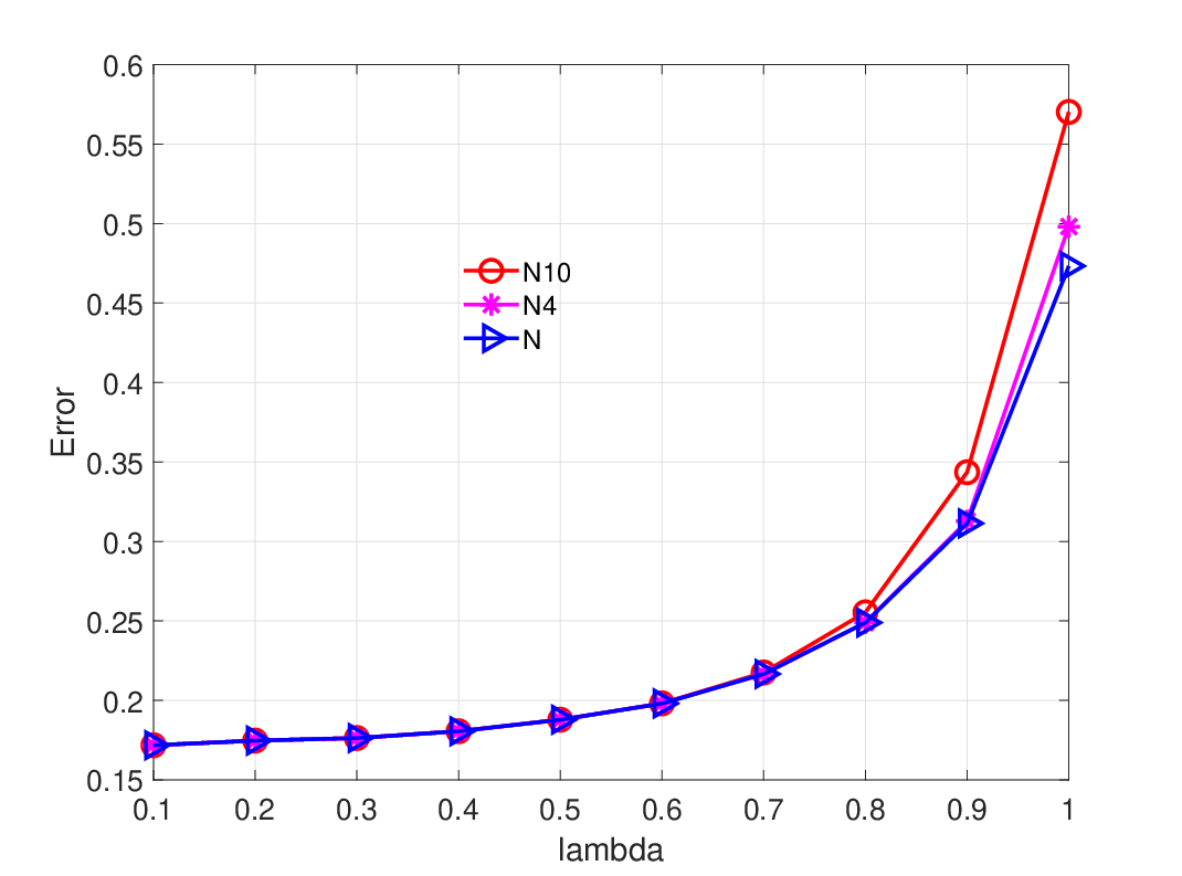
As can be intuitively guessed, the performance of the proposed interval-valued estimators depends on the properties of the RLS reference identifier which in turn are determined by the richness of the data and the user-defined parameters such as $P(0)$ and $\lambda$ . In particular, it is interesting to study the impact of the forgetting factor $\lambda\in\mathopen{]}0,1\mathclose{]}$ . In general, for point-valued estimation, such a parameter is selected, to be close to $1$ in order to smooth the trajectories of $\theta$ in (9). In contrast, the recursive interval-valued estimator (38)-(39) tends to perform better when $\lambda$ is small. To see this consider Figure 3 where we have plotted the final interval width $\overline{\theta}(N)-\underline{\theta}(N)$ achieved by the estimator (38)-(39). Again only the estimates related to the first component of the parameter vector are represented. We consider the estimator (38)-(39) with $\underline{\xi}=c_{\theta}-\hat{r}_{\theta,m}$ and $\overline{\xi}=c_{\theta}+\hat{r}_{\theta,m}$ as defined in (28) and (30) for $m\in\left\{20,50,N\right\}$ . The results are indeed averages over $100$ independent simulations. What this reveals is that the estimator’s asymptotic performance depends on the forgetting factor in the sense that the width of the estimated interval is all the smaller as the forgetting factor $\lambda$ is small. This behavior can be explained by the fact that a small $\lambda$ in the RLS may cause the estimates $(c_{\theta},\hat{r}_{\theta,m})$ to fluctuate substantially hence favoring the event that the associated interval jumps occasionally to a small value. We can further observe that for small values of the forgetting factor (e.g., $\lambda\leq 0.6$ in Figure 3), all truncation orders $m$ tend to perform equally well. This suggests an important feature of the proposed estimation framework for practical implementation: provided the exciting input $\left\{u(t)\right\}$ is sufficiently rich and $\lambda$ is then taken small enough, the computational complexity of the estimators can be reduced to the minimum by selecting a small truncation horizon $m$ .

6.2 Linear Time Varying system

We now consider a model of the form (1) where the parameter vector $\theta^{\circ}$ is time-varying with dynamics defined as in (40) where it is assumed that $\delta(t)$ belongs to an interval given by $c_{\delta}(t)=0$ and $r_{\delta}(t)=[\begin{matrix}0.10&0.05&0.04&0.01\end{matrix}]^{\top}$ for all $t$ . For the simulation, we generate a sequence $\left\{\delta(t)\right\}$ in this interval such that $\delta(t)=r_{\delta}(t)\sin(2\pi t/30)$ . The other settings remain the same as previously defined in the beginning of Section 6 except the forgetting factor which is now set to $0.1$ (recall that as discussed earlier, the estimate is tighter when $\lambda$ is small). Consider applying the estimator (47)-(48) with inputs $\underline{\xi}=c_{\theta}-\hat{r}_{\theta,m}$ and $\overline{\xi}=c_{\theta}+\hat{r}_{\theta,m}$ as defined in (28) and (30) for $m\in\left\{5,N\right\}$ . The outcome of this experiment is depicted in Figure 4. For a value of $\lambda$ as small as $0.1$ , the estimated interval appears to be very tight. Moreover, all values of the truncation horizon $m$ give almost the same performance in this case.

7 Conclusion

In this paper, we have presented a recursive interval-valued estimation framework for the identification of linearly parametrized models. The main idea of the method is to carefully bound the error generated by a certain reference adaptive algorithm, for example the recursive least squares. However the smallest interval-valued estimator we discussed turns out to be computationally costly to implement in an online scenario. We therefore turn to an alternative family of (over)-estimators which exhibits a trade-off between the achievable performance of and the price to pay for it in computational load. Two cases have been studied: one where the to-be-estimated parameter vector is constant and a more general situation where it is possibly time-varying. In the first case, we further show that the estimated interval size can be made monotonically decreasing. In the second, this monotonic property cannot be systematically achieved (as this depends on the change rate of the parameters) but the width of the estimated interval can be made very small by an appropriate design of the reference point-value identifier. For example, we have observed in simulation that when the reference identifier is the RLS algorithm, the performance of the estimator improves if the forgetting factor is small.
Future work may concern the extension of the proposed interval-valued estimation framework to systems whose models are nonlinear in the parameters.

References

[1] L. Bako. Adaptive identification of linear systems subject to gross errors. Automatica, 67:192–199, 2016.
[2] L. Bako and V. Andrieu. Interval-valued estimation for discrete-time linear systems: application to switched systems. https://arxiv.org/abs/1912.10770, 2018.
[3] L. Bako and V. Andrieu. Interval-valued state estimation for linear systems: the tightest estimator and its relaxations. Automatica, 106:168–177, 2019.
[4] S. Brüggemann and R. R. Bitmead. Exponential convergence of recursive least squares with forgetting factor for multiple-output systems. Automatica, 124:109389, 2021.
[5] L. Chisci, A. Garulli, A. Vicino, and G. Zappa. Block recursive parallelotopic bounding in set membership identification. Automatica, 34:15–22, 1998.
[6] G. C. Goodwin and K. S. Sin. Adaptive Filtering Prediction and Control. Dover Publications Inc., Mineola, New York, 2009.
[7] P.-O. Gutman. Online parameter interval estimation using recursive least squares. International Journal of Adaptive Control and Signal Processing, 8:61–72, 1994.
[8] L. Jaulin, M. Kieffer, O. Didrit, and E. Walter. Applied interval analysis. Springer, London, 2001.
[9] R. M. Johnstone, C. R. Johnson Jr, R. R. Bitmead, and B. D. Anderson. Exponential convergence of recursive least squares with exponential forgetting factor. Systems & Control Letters, 2:77–82, 1982.
[10] M. Kieffer and E. Walter. Interval analysis for guaranteed non-linear parameter and state estimation. Mathematical and Computer Modelling of Dynamical Systems, 11:171–181, 2005.
[11] M. Lauricella and L. Fagiano. Set membership identification of linear systems with guaranteed simulation accuracy. IEEE Transactions on Automatic Control, 65:5189–5204, 2020.
[12] M. Milanese, J. Norton, H. Piet-Lahanier, and E. W. (Eds). Bounding approaches to system identification. Springer Science & Business Media, 2013.
[13] M. Milanese and C. Novara. Unified set membership theory for identification, prediction and filtering of nonlinear systems. Automatica, 47:2141–2151, 2011.
[14] R. E. Moore, R. B. Kearfott, and M. J. Cloud. Introduction to Interval Analysis. SIAM, 2009.
[15] X. F. Sun, H. Y. Zhang, and Y. Z. Fan. Recursive dual-linear-programming approach for parameter-uncertainty-interval estimation., 150(3), 303-310. IEE Proceedings-Control Theory and Applications, 150:303–310, 2003.
[16] G. Tao. Adaptive control design and analysis. John Wiley & Sons, 2003.
[17] E. van Kampen, Q. Chu, and J. Mulder. Interval analysis as a system identification tool. In Advances in Aerospace Guidance, Navigation and Control, Springer, Berlin, Heidelberg, pages 333–343, 2011.
[18] A. Vicino and G. Zappa. Sequential approximation of feasible parameter sets for identification with set membership uncertainty. IEEE Transactions on Automatic Control, 41:774 –785, 1996.
[19] E. Walter and H. Piet-Lahanier. Recursive robust minimax estimation for models linear in their parameters. IFAC Proceedings Volumes, 25:215–220, 1992.

	$\displaystyle\hat{r}_{\theta,m}(t)=$	$\displaystyle\Big(\prod_{\ell=1}^{\alpha(t)}\Big\|\Phi\big(t-(\ell-1)m,t-\ell m\big)\Big\|\Big)\hat{r}_{\theta,m}(\beta(t))$
		$\displaystyle+\sum_{j=1}^{\alpha(t)}\>\sum_{k=t-jm+1}^{t-(j-1)m}\>\Big(\prod_{\ell=1}^{j-1}\Big\|\Phi\big(t-(\ell-1)m,t-\ell m\big)\Big\|\Big)\times\ldots$
		$\displaystyle\ldots\times\Big\|\Phi\big(t-(j-1)m,k\big)q(k)\Big\|r_{v}(k)$

$\displaystyle\hat{r}_{\theta,m}(t)=$	$\displaystyle\Big(\prod_{\ell=1}^{\alpha(t)+1}\Big\|\Phi\big(\kappa(t,\ell-1),\kappa(t,\ell)\big)\Big\|\Big){r}_{\theta}(0)$	(32)
	$\displaystyle+\sum_{j=1}^{\alpha(t)+1}\>\sum_{\kappa(t,j)+1}^{\kappa(t,j-1)}\>\Big(\prod_{\ell=1}^{j-1}\Big\|\Phi\big(\kappa(t,\ell-1),\kappa(t,\ell)\big)\Big\|\Big)\times\ldots$
	$\displaystyle\ldots\times\Big\|\Phi\big(\kappa(t,j-1),k\big)q(k)\Big\|r_{v}(k)$

		$\displaystyle\prod_{\ell=1}^{\alpha(t)+1}\Big\|\Phi\big(\kappa(t,\ell-1),\kappa(t,\ell)\big)\Big\|$
		$\displaystyle=\Big(\prod_{i=1}^{\alpha(t)}\Big\|\Phi\big(t-(i-1)m,t-im\big)\Big\|\Big)\left\|\Phi(t-\alpha(t)m,0)\right\|$
		$\displaystyle\geq\Big\|\Phi\big(t,t-m\big)\Phi\big(t-m,t-2m\big)\cdots\Phi\big(t-\alpha(t)m,0\big)\Big\|$
		$\displaystyle=\big\|\Phi\big(t,0\big)\big\|,$

	$\displaystyle\hat{r}_{\theta,m}(t)$	$\displaystyle\geq\big\|\Phi\big(t,0\big)\big\|r_{\theta}(0)+\sum_{j=1}^{\alpha(t)}\>\sum_{k=t-jm+1}^{t-(j-1)m}\>\big\|\Phi\big(t,k\big)q(k)\big\|r_{v}(k)$
		$\displaystyle+\sum_{k=1}^{t-\alpha(t)m}\|\Phi(t,k)q(k)\|r_{v}(k)$
		$\displaystyle=\big\|\Phi\big(t,0\big)\big\|r_{\theta}(0)+\sum_{k=1}^{t}\>\big\|\Phi\big(t,k\big)q(k)\big\|r_{v}(k)$
		$\displaystyle=r_{\theta}(t)$

	$\displaystyle\left\\|\hat{r}_{\theta,m}(t)\right\\|_{2}$	$\displaystyle\leq\Big(\prod_{i=1}^{\alpha(t)+1}\Big\\|\Phi\big(\kappa(t,i-1),\kappa(t,i)\big)\Big\\|_{F}\Big)\left\\|{r}_{\theta}(0)\right\\|_{2}$
		$\displaystyle+\sum_{j=1}^{\alpha(t)+1}\!\!\sum_{k=\kappa(t,j)+1}^{\kappa(t,j-1)}\>\Big(\prod_{\ell=1}^{j-1}\Big\\|\Phi\big(\kappa(t,\ell-1),\kappa(t,\ell)\big)\Big\\|_{F}\Big)\times\ldots$
		$\displaystyle\ldots\times\Big\\|\Phi\big(\kappa(t,j-1),k\big)\Big\\|_{F}\left\\|q(k)\right\\|_{2}\left\\|r_{v}(k)\right\\|_{2}$