Excitations in the higher lattice gauge theory model for topological phases III: the (3+1)-dimensional case
Abstract
In this, the third paper in our series describing the excitations of the higher lattice gauge theory model for topological phases, we will examine the 3+1d case in detail. We will explicitly construct the ribbon and membrane operators which create the topological excitations, and use these creation operators to find the pattern of condensation and confinement. We also use these operators to find the braiding relations of the excitations, and to construct charge measurement operators which project to states of definite topological charge.
I Introduction
Over the past decade, there has been significant consideration given to topological phases in 3+1d, in addition to the 1+1d and 2+1d cases that have been more heavily studied in the past. So far, results for 3+1d topological phases range from the construction of classes of commuting projector models Walker and Wang 2012; Wan et al. 2015; Williamson and Wang 2017; Bullivant et al. 2017 to a potential classification of the bosonic phases in the absence of symmetry Lan et al. 2018; Lan and Wen 2019. 3+1d phases are intriguing for several reasons. Firstly, we live in a 3+1d world, and so there is a natural interest in studying such phases. Secondly, the properties of 3+1d topological phases are quite different from their 2+1d cousins. Unlike their 2+1d counterparts, point-like particles in 3+1d are not expected to have non-trivial braiding with each-other (outside of the usual bosonic and fermionic cases) Doplicher et al. 1971; Doplicher et al. 1974. However, in these higher-dimensional phases there exist loop-like excitations with non-trivial loop-braiding properties, so that exchange processes involving the loop-like excitations can result in a non-trivial transformation for the state of the system. Unfortunately, at present there are few examples of toy models where these loop-like excitations are constructed explicitly and the properties of the excitations (both point-like and loop-like) are studied in more depth. In this series of papers, we study one such toy model Bullivant et al. 2017, based on higher lattice gauge theory Pfeiffer 2003; Baez and Huerta 2010; Gukov and Kapustin 2013; Kapustin and Thorngren 2014; Kapustin and Thorngren 2017; Bullivant et al. 2017, and aim to provide a detailed description of the excitations, and the conserved topological charge which they carry.
As we have already seen in Refs. Huxford and Simon 2023a; Huxford and Simon 2023b, the Hamiltonian model for topological phases based on higher lattice gauge theory Bullivant et al. 2017 hosts rich physics, including non-trivial loop braiding (in the 3+1d case), condensation and confinement. In Ref. Huxford and Simon 2023a, we gave a brief qualitative description of these features, while in Ref. Huxford and Simon 2023b we examined the 2+1d model. Now we will give a more explicit and mathematically detailed treatment of the 3+1d model, with full proofs presented in the Supplemental Material. Our approach focuses heavily on the so-called ribbon and membrane operators, which produce (as well as move and annihilate) the point-like and loop-like excitations of the model respectively. Because loops are extended objects, they sweep through a surface as they move, rather than just a line as point particles would. Therefore, to produce and move loop excitations we need an operator that is defined across a general membrane rather than a line or ribbon. The ribbon and membrane operators can be used to find the braiding statistics Kitaev 2003; Levin and Wen 2005 of the excitations, while closed ribbon and membrane operators can be used to measure topological charge Bombin and Martin-Delgado 2008. In addition, certain properties of the excitations, such as whether they are confined or not, can be obtained directly from these operators. In this paper, we therefore aim to provide and justify the mathematical forms of the ribbon and membrane operators, and demonstrate how we can extract all of the previously mentioned information about the excitations from them.
I.1 Structure of this paper
In this paper, we will consider the 3+1d model in various cases (a summary of these cases is presented in Section II, along with a brief reminder of the Hamiltonian model). For each case we define the membrane operators and find the effects of braiding in turn, before moving on to the next case. In Sections III and IV we consider the case where one of the maps describing the model, , is trivial (Case 1 from Table 1). In Section III we construct the ribbon and membrane operators for the theory and discuss the pattern of condensation and confinement exhibited by the excitations that they produce. In Section IV we use these operators to work out the braiding properties of these excitations, which involves passing loop or point particles through loops. In Sections V and VI we repeat the construction of ribbon operators and the braiding for another special case, called the fake-flat case (Case 3 from Table 1), while in Sections VII and VIII we repeat it for another special case (Case 2 from Table 1), which generalizes the trivial case.
Having found the membrane operators and effects of braiding, in Section IX we move on to consider the topological charges of the model. These topological charges are conserved quantities carried by the excitations of the model. In 2+1d, to measure the topological charge in a spatial region, we simply put an operator on the boundary of that region. This boundary will be topologically equivalent to a circle (or multiple circles). However, in 3+1d there are more topologically distinct surfaces which can enclose our regions of interest. We can use these different surfaces to measure the loop-like and point-like charge carried by the excitations. Using a sphere as our surface of measurement, we can determine the point-like charge contained within the sphere. We present the corresponding charge measurement operators in Section IX.1, and also find the charge carried by some simple excitations. However, to measure loop-like charge we need some surface with non-contractible loops. An important example is the torus, which we look at in some detail in Section IX.2. We compare the number of topological charges that we can measure with the torus to the ground state degeneracy of the 3-torus and find that they are equivalent, in the broad cases that we look at, as previously reported in Ref. Bullivant and Delcamp 2020. Finally, in Section X, we summarize our results and propose further avenues of research based on this work.
In the Supplemental Material, we present the proofs of our results that were too lengthy to include in the main text. We demonstrate the commutation relation between the energy terms and the ribbon and membrane operators in Section S-I (using some results from the 2+1d case discussed in Ref. Huxford and Simon 2023b). Then in Section S-II we demonstrate that the non-confined ribbon and membrane operators are topological, meaning that we can deform them through unexcited regions of space without affecting their action, provided that we keep the locations of any excitations they produce fixed. In Section S-III, we show that some of the magnetic loop excitations are condensed, and can be produced by operators only acting near the excitations (meaning that they cannot carry loop-like topological charge). Next, in Section S-IV we find the braiding relations of the various excitations by explicitly calculating the appropriate commutation relations between the membrane and ribbon operators. Finally, in Section S-V we construct the measurement operators for topological charge and demonstrate that they are projectors.
II Summary of the model
In this section we will remind the reader of the Hamiltonian model we are studying, the higher lattice gauge theory model introduced in Ref. Bullivant et al. 2017. We hope that this will provide a convenient place for the reader to refer back to for definitions of the various terms in the Hamiltonian, along with several useful identities.
We are considering the model defined on a 3d lattice, representing the spatial degrees of freedom, with a Hamiltonian controlling the time evolution. The edges of the lattice are directed, while the plaquettes have a circulation and a base-point (a privileged vertex which we can think of as the start of the circulation). The edges are labeled by elements of a group , and the plaquettes are labeled by elements of a second group, . These groups are part of a crossed module, which consists of the two groups and two maps, and . Here is a group homomorphism from to , while is a group homomorphism from to the automorphisms on . That is, for each element , is a group isomorphism from to itself (so for , is an element of ). These maps satisfy two additional constraints, called the Peiffer conditions Pfeiffer 2003; Baez 2002; Bullivant et al. 2017:
| (1) | ||||
| (2) |
The Hamiltonian is given by a sum of projectors, with terms for the vertices, edges, plaquettes and blobs (3-cells) of the lattice Bullivant et al. 2017:
| (3) |
The vertex terms are a sum of vertex transforms, and can be thought of as projecting to states that are 1-gauge invariant. That is
where the vertex transforms have the algebra , which implies that . This ensures that the ground states (which are eigenstates of with eigenvalue one) are invariant under the vertex transforms:
As for the specific action of the vertex transforms, they act on the edges adjacent to the vertex, as well as any plaquette whose base-point is that vertex. For an edge (initially labeled by ) or plaquette (initially labeled by ), we have
| (4) |
Similarly, the edge term is a sum of edge transforms (2-gauge transforms)
which satisfy a similar algebra to the vertex transforms: . This ensures that individual edge transforms can be absorbed into the corresponding edge term, and into the ground state: and . An edge transform applied on an edge acts on the label of edge itself, as well as the labels of the adjacent plaquettes:
| (5) |
Here is the source of edge , which is the vertex attached to that points away from (with the vertex on the other end of being called the target). is the path element for the path from the base-point of plaquette to this source, running around the plaquette and aligned with the plaquette. On the other hand is the path element for the path around the plaquette from to , but this time anti-aligned with the plaquette.
The next energy term is the plaquette term, , which enforces so-called fake-flatness. This is similar to the plaquette term from Kitaev’s Quantum Double model, in that it restricts which labels the boundary of a plaquette can have. Unlike the term from the Quantum Double model however, the plaquette term in higher lattice gauge theory relates the label of the boundary to the surface label of the plaquette itself, rather than requiring the boundary label to be trivial as for the Quantum Double model. For a plaquette whose boundary (starting at the base-point and aligned with the circulation of the plaquette) has path label , and whose surface label is , the plaquette term acts as
| (6) |
A plaquette which satisfies this Kronecker delta is called fake-flat, and a surface made from fake-flat plaquettes is also called fake-flat. Such a fake-flat surface will satisfy a similar condition on its surface and boundary labels. As we showed in Ref. Huxford and Simon 2023b, for a surface whose constituent plaquettes satisfy fake-flatness, the overall surface element will satisfy
where is the group element associated to the boundary of and the total surface element is constructed by combining individual surface elements, as explained in Ref. Bullivant et al. 2017 and as we will summarize shortly. Note that this fake-flatness condition enables the presence of closed paths with non-trivial label in the ground state (indeed such closed paths are created by the edge transforms), indicating that some magnetic fluxes proliferate in the ground state and so are condensed.
The final energy term is the blob term, , which enforces that the surface element of the boundary of the blob (calculated from the plaquettes on that blob using the rules for combining surfaces explained in Ref. Bullivant et al. 2017, which we will describe shortly) is equal to the identity element . That is
| (7) |
for blob with surface element .
A key idea in the higher lattice gauge theory model is that we can compose edges into paths and plaquettes into surfaces, with composite objects appearing throughout the description of the model as well as in the ribbon and membrane operators. We will therefore briefly review the rules for this kind of combination. First, consider composing edges into paths. If two edges (or more general paths) lie end-to-end, then we can combine them into one path, with a group label given by the product of the elements for the two edges. Then to combine multiple edges into a path, we take a product of all of the constituent edge labels, with the first edge on the path appearing on the left of the product. If one or more of the edges points against the path (for example, the edges labeled by and in Figure 1), then we include the edge label in the path element with an inverse.
Next consider composition of plaquettes, or more generally surfaces. Surfaces have both an orientation and a privileged vertex, called the base-point, which we can view as the start of the circulation. We represent this by drawing a circulating arrow in the plaquette which connects to the boundary at the base-point, as illustrated in Figure 2. When we combine two adjacent plaquettes, we must ensure that the base-points and orientations of the plaquettes both agree. If they do, as in the example shown in Figure 2, we can combine the plaquettes into a single surface whose label is a product of the two plaquettes. Contrary to the case of paths, the plaquette appearing first in the circulation is represented in the rightmost position of the product.
While this simple procedure works if the base-points and orientations of the two plaquettes agree, we will often want to combine adjacent plaquettes for which this is not the case (similar to how we want to combine edges into paths even if their orientations are not all aligned). In this case, we need a procedure for changing the base-point and orientation of a plaquette, and describing the label the plaquette would have with this new decoration. As described in Ref. Huxford and Simon 2023a, we can reverse the orientation of a plaquette (while keeping its base-point fixed) by inverting its group label, as shown in Figure 3. If we want to move the base-point along a path , as shown in Figure 4, then we must act on that plaquette element with , so that the plaquette label goes from to . When moving the base-point in this way, we can either move it along the boundary of the plaquette, as shown in the bottom-left of Figure 4, or we can move it away from the boundary, as shown in the top-right of Figure 4. Combining these two procedures, we see that the general formula for the label of a composite surface is
| (8) |
where the are the constituent plaquettes; is the original base-point of plaquette ; is the base-point of the combined surface; and is 1 if the circulation of plaquette matches the surface and otherwise. Note that this formula hides certain complexities, such as the order of the product and the precise definition of the paths , but often we care about situations where these details do not matter (for example if is Abelian the order does not matter, and if the surface is also fake-flat then the paths only need to be defined up to deformation).
One useful way of checking whether we have correctly composed two surfaces it to examine the boundary of the combined surface. The boundary of a surface made by composing two other surfaces is the product of the two individual boundaries, once we have ensured that the orientations and base-points of the two surfaces agree. This product of the boundaries follows from the rules for composing paths given previously. As an example, consider Figure 5. The boundary of the left surface () in the top image is (note that the boundary starts at the base-point and follows the orientation of the plaquette), while the boundary of the right surface () is . Here represents an edge, rather than an edge label. The boundary of the combined surface is therefore . This is the path shown in red in the upper image of Figure 5. We can simplify this path by removing the section , to give the boundary shown in the lower image. This rule for combining boundaries ensures that the total surface satisfies fake-flatness, if the two constituent surfaces do. If the surface label of surface (for or 2) is , and the boundary bd has label , then the surface satisfies fake-flatness when
and the surface satisfies fake-flatness when
The combined surface has label and boundary label (note the opposite order of composition for the paths and surfaces). If the two constituent surfaces satisfy fake-flatness, then the combined surface label satisfies
so the total surface satisfies a fake-flatness condition, as we claimed earlier.
Next, we want to remind the reader of the various special cases in which we consider the model. In the most general case of the model, the projectors in the Hamiltonian (specifically the edge and blob terms) no longer commute Bullivant et al. 2017. Furthermore, there are inconsistencies with regards changing the branching structure of the lattice (reversing the orientation of edges or plaquettes, or moving the base-points of plaquettes around), as we showed in the Appendix of Ref. Huxford and Simon 2023a. This only occurs when is non-trivial and there are fake-flatness violations (i.e., plaquette excitations), so the ground state space is always well-defined. This may be similar to how the plaquette terms in the string-net model become poorly defined when neighbouring vertex terms are not satisfied and are usually set to zero in such cases Levin and Wen 2005. Regardless, these inconsistencies make it difficult to define the plaquette excitations, which form flux tubes. We therefore consider the higher lattice gauge theory model in various special cases that remove these inconsistencies, or at least make them more manageable. In the first such special case (Case 1 in Table 1), we take the map to be trivial, so that each map is the identity map ( for all and ). This leads to a model very similar in character to a 3+1d version of Kitaev’s Quantum Double model, but with some additional excitations (and with condensation and confinement). Because of the Peiffer conditions, taking this form for enforces that be an Abelian group and maps onto the centre of . In the second special case (Case 2 in Table 1), we instead take these properties as our starting point, allowing to be general, subject to the constraint that is Abelian and maps to the centre of . In the final case (Case 3 in Table 1), we do not place any conditions on our crossed module, but instead restrict the Hilbert space to only include fake-flat states (states where all of the plaquette terms are satisfied). This prevents any inconsistencies, but means that some of the excitations are missing.
| Full | ||||
| Case | Hilbert | |||
| Space | ||||
| 1 | Abelian | Trivial | centre() | Yes |
| 2 | Abelian | General | centre() | Yes |
| 3 | General | General | General | No |
We mentioned that when is trivial, the higher lattice gauge theory model becomes similar to a 3+1d version of Kitaev’s quantum double model, i.e., to regular lattice gauge theory. Indeed, there are two subcases where the model is equivalent to lattice gauge theory. The first of these is when the group is the trivial group and so maps to the identity of . In this case, the blob and edge energy terms become trivial, while the vertex and plaquette terms become the corresponding lattice gauge theory terms. This directly gives the lattice gauge theory Hilbert space and Hamiltonian. The other limit is where the group is trivial (which also implies that maps to the identity element, because only has one element). In this case, the vertex and plaquette terms become trivial. Under a change of basis from group elements of to irreps of , the remaining energy terms become the lattice gauge theory terms on the dual lattice, where the group is the group of irreps of . Specifically, the blob energy term of higher lattice gauge theory becomes the vertex term of lattice gauge theory, while the edge term becomes the plaquette term. More generally, if both groups and are non-trivial, but is trivial and maps to the identity of , we can see that each of the energy terms given in Equations 4-7 only affects the variables corresponding to one group. This means that these variables decouple and we can think of higher lattice gauge theory as two decoupled lattice gauge theory models in this case. This also helps us to interpret more general cases of the model. If we change to map to a larger subgroup, the two lattice gauge theories interact and produce condensation and confinement, as we will discuss later.
III Ribbon and membrane operators in the trivial case
Firstly, we consider Case 1 from Table 1, the case where is trivial (), which enforces that is Abelian.
III.1 Electric excitations
The first type of excitation to consider is the electric excitations. The ribbon operators that produce the electric excitations in 3+1d have the same form as the ones for the 2+1d case that we considered in Ref. Huxford and Simon 2023b. That is, an electric ribbon operator measures the group element of a path and assigns a weight depending on the measured group element. As we claimed in Ref. Huxford and Simon 2023a, an electric ribbon operator applied on a path has the form
| (9) |
where is an arbitrary set of coefficients for each group element and different choices for these coefficients describe different operators in a space of ribbon operators. A useful basis for this space has basis operators that are labeled by irreps of the group and the matrix indices for that irrep. These basis electric ribbon operators have the form
| (10) |
where is an irrep of , is the associated matrix representation of element , and and are the matrix indices. As we proved in Ref. Huxford and Simon 2023b (in the 2+1d case, although the proof also holds for 3+1d), the operators labeled by non-trivial irreps excite the vertices at the ends of the path, whereas the operator labeled by the trivial irrep is the identity operator (which of course does not create any excitations). In addition, just as in the 2+1d case discussed in Ref. Huxford and Simon 2023b, the irreps that have non-trivial restriction to the image of label confined excitations. The electric ribbon operators labeled by such irreps cause the edges along the path to be excited, so the excitations produced at the ends of the ribbon are confined.
III.2 Magnetic excitations
Unlike the electric excitations, the magnetic excitations in 3+1d are significantly different from their counterparts in 2+1d. Whereas in 2+1d the magnetic excitations are point particles that are produced in pairs by a ribbon operator (as we described in Ref. Huxford and Simon 2023b), in 3+1d the elementary magnetic excitation is a “flux tube” at the boundary of a membrane. That is, the magnetic excitations are loop-like. We can see that the magnetic excitations must be loop-like by trying to excite a single plaquette. We try changing the value of a single edge belonging to that plaquette. However, as shown in Figure 6, in 3+1d each edge belongs to multiple plaquettes (as opposed to two plaquettes when there are only two spatial dimensions). Therefore, changing the label of an edge excites all of the plaquettes around that edge. We can then put one of these plaquettes back into a lower energy state by changing the label of another edge on that plaquette, but this in turn excites all of the other plaquettes attached to that edge (see the second image in Figure 6). We see that these excited plaquettes lie on a closed loop that pierces their centres, as shown by the blue loops in Figure 6. This is made more clear by considering changing more edges. Instead of changing edges along a line, we consider changing edges across some surface (such as the four edges shown in the third image of Figure 6, which lie on a square). Changing these edges excites the plaquettes on the boundary of that surface, much as the ribbon operators in 2+1d excite particles at the ends of some path.

The fact that we produce a loop excitation by changing edges across a surface rather than just along a path indicates that our creation operator is a membrane operator. While we have given a rough idea of the action of the membrane operator in the above discussion, we will now be more specific. In order to define the operator that produces a magnetic excitation, we must specify the region (the “membrane”) that this operator acts on. First we specify a membrane that passes through the centres of plaquettes and cuts through edges. The edges cut by the membrane (“cut edges”) are acted on by the operator, as shown in Figure 7. This membrane is called the dual membrane, and is analogous to the dual path for the magnetic ribbon operator in 2+1d. In addition to the dual membrane, we must specify a “direct membrane”. The cut edges terminate on this membrane. That is, the direct membrane contains one vertex at the end of each of the cut edges, as shown in Figure 7 (in special cases, with tightly folded membranes, both ends may be on the direct membrane and an edge may be cut twice by the dual membrane). We must also specify a set of paths to the vertices on the direct membrane. These paths go from a common start-point to the base of each cut edge (that is, to the vertex that lies on the direct membrane). We call this common start-point of the paths the start-point of the membrane or of the membrane operator. These features of the membrane operator are illustrated in Figure 7.
The fact that we specify two membranes as part of the magnetic membrane operator indicates that our “membrane operator” really acts on a “thickened” membrane, much as the ribbon operators in 2+1d can be considered as acting on thickened strings, that is on ribbons (i.e., their support has some finite thickness). Regardless, we will continue to refer to these operators as membrane operators. This unfortunately means that our use of the term membrane is somewhat ambiguous. Sometimes we mean a “thickened membrane” and sometimes just an unthickened membrane. Generally we try to use membrane to refer to the region on which our membrane operators act, whether those regions are thickened or otherwise. If we want to refer to a surface that may not be part of a membrane operator, we will call this a surface. If we want to refer to part of a thickened membrane, we will use the terms direct and dual membranes.
Having specified these features of the membrane, we can now describe the action of the magnetic membrane operator. The membrane operator acts on the edges cut by the dual membrane, in a way that depends on the direct membrane and the paths we defined. This is analogous to how the action of the magnetic ribbon operator in the 2+1d case depends on a direct path and a dual path (see Ref. Huxford and Simon 2023b). The membrane operator is labeled by a group element , but the label of each cut edge is left-multiplied by or right-multiplied by the inverse, where is the group element associated to the path specified from the start-point to the vertex on the direct membrane that is attached to the cut edge . Whether left-multiplication or right-multiplication by the inverse is used depends on the orientation of the edge. The edge label is left-multiplied if the edge points away from the direct membrane (as with the example edge in Figure 7) and is right-multiplied by the inverse element if it points towards the membrane. That is, the action of the membrane operator on an edge with initial label is given by
| (11) |
The only difference compared to the action of the magnetic ribbon operator in 2+1d is that the operator acts on a general membrane, rather than just a ribbon. In particular, this means that instead of having a direct path along a ribbon, we have multiple paths across a membrane. For a given edge , there are many potential choices for the path from the start-point to the edge. However, the action of the membrane operator is unaffected by deforming any of these paths over a region satisfying fake-flatness. This is because deforming the path in this way only changes the path element by an element in . This factor of is in the centre of and so it does not affect the expression , which just gains a factor of and a factor of which can be moved together and cancelled.

Now that we have described the action of the membrane operator, we can discuss which of the energy terms are excited by the membrane operator. Firstly, note that if the membrane operator is labeled by then the membrane operator is just the identity operator and so will not excite any of the energy terms. From now on we will assume that we are talking about a membrane operator labeled by some non-trivial element of . In this case the membrane operator excites the “boundary plaquettes”, which are plaquettes where only one edge on the plaquette is changed by the membrane operator (rather than two for the “bulk” plaquettes). These boundary plaquettes lie around the perimeter of the membrane (they are the red plaquettes in Figure 7) and we can construct a closed path around the boundary of the dual membrane which passes through these plaquettes.
In addition to these plaquettes, the magnetic membrane operator may also excite the privileged start-point vertex that we defined previously, just as we saw in the 2+1d case for the magnetic ribbon operator in Ref. Huxford and Simon 2023b. In order for the magnetic membrane operator to produce an eigenstate of this vertex energy term when acting on an initially unexcited region, we need to construct a linear combination of the magnetic membrane operators labeled by elements of . If the coefficients for this linear combination are a function of conjugacy class (that is we have an equal sum over all elements of the conjugacy class), the vertex is not excited. On the other hand, if the coefficients within each conjugacy class sum to zero, then the vertex is excited. In any other case (such as when we do not take a superposition of our operators), the start-point is neither definitely excited nor definitely unexcited, because we do not produce an energy eigenstate. While in Figure 7 the start-point is next to the loop-like excitation (at the edge of the membrane), the start-point can be displaced any distance from the excited loop (or even away from the membrane). The position of the start-point can be interpreted in terms of the picture of the ribbon and membrane operators creating and moving excitations. We can think of the membrane as corresponding to the process where we nucleate a loop at the start-point and then grow and move the loop along the membrane to its final position. The fact that the start-point may be excited far from the loop suggests that it can be treated as an additional particle. Therefore, when we produce a loop, we may also have to produce a point-particle. This is similar to how point-like charges must be produced in pairs in order to conserve topological charge. Indeed we will see in Section IX.1 that some loop-like excitations carry a non-trivial “point-like” conserved charge, which must be balanced by the charge carried by the additional excitation at the start-point.
The magnetic membrane operator described above is a creation operator for our flux tube, which runs around the perimeter of the membrane. The membrane operator creates a flux tube (and its associated vertex excitation) from the vacuum. Another relevant operator is the one that moves an existing flux tube to a new position. The movement operator can be thought of as an ordinary membrane operator, but with an additional hole whose boundary fits the loop that we wish to move. To see that this is a movement operator, consider splitting a creation operator into two parts, an inner part, which is another creation operator, and an outer part applied on a membrane equivalent to a tube or annulus, as shown in Figure 8. We know that the overall membrane operator produces and moves an excitation to the boundary of the outer part, while the inner part produces and moves an excitation to the boundary of the inner part. Because the overall membrane operator is a combination of the inner membrane operator and outer membrane operator, this means that the outer membrane operator must take the excitation from the boundary of the inner part and move it to the boundary of the outer part, to match the action of the total membrane operator.
For instance, consider the example shown in Figure 8. In this figure, the yellow membranes indicate the membrane on which the operator is applied (so that if we zoomed in we would see the structure from Figure 7). The yellow spheres are the start-points for the membranes (note that they are all in the same position). The opaque tori indicate the excitations they create. The two membranes on the right are displaced horizontally to indicate an order in which operators are applied, rather than spatial displacement. On the left-hand side of the Figure, we have an operator that simply creates and moves an excitation to the final position (indicated by the red torus). We can split this operator into the two operators shown on the right-hand side. The rightmost operator on the right-hand side is the inner part of the original membrane operator and so is another flux creation operator. Therefore, this operator also creates an excitation and moves it to its boundary, the lower red torus. In order for this decomposition of operators to agree with the total operator on the left-hand side, we see that the middle operator, which represents the outer part of the original membrane operator, must move an excitation from the lower position (the yellow torus) to the final position (the red torus). While in this context the outer membrane operator moves an existing excitation, we can also apply it when there are no existing excitations. In this case the operator instead creates two opposite fluxes at the two ends of the operator. We therefore do not need to distinguish between movement and creation operators, because the movement operators are also creation operators, although they create multiple loop-like excitations.

More generally, we can put many holes in the membrane to produce many loop excitations. Indeed, we can think of the membrane operator that we originally defined as a closed, topologically spherical membrane with a single hole in it. Then the excited loops (or single loop in the ordinary case) are at the boundaries of these holes. A topologically spherical membrane operator would produce no excitations. Indeed, as we prove in Section S-II.4 in the Supplemental Material, such a spherical membrane operator will act trivially if it is contractible and encloses no other excitations.
When producing an excitation in a given location, there are many choices for the position of the membrane. This is because the excitation is produced at the boundary of the membrane and many different membranes share the same boundary. However, the membrane operator is topological in the following sense. We can freely deform the membrane on which the operator is applied through the lattice, while keeping the positions of any excitations produced by the operator fixed, as long as we do not deform the membrane over any existing excitations. When we do this, the action of the membrane operator is preserved. That is, given an initial state and a magnetic membrane operators applied on a membrane , if we can deform the membrane into a new membrane without crossing any excitations in , or moving the excitations produced by , then we have . This means that, like the ribbons in 2+1d, the membrane is invisible when acting on the ground state; it does not matter precisely where we put the membrane. However, when we act on a state that already has excitations, the position may matter. Indeed this fact is vital when considering braiding and leads to the non-trivial braiding relations that we will see in Section IV.
It is not just the magnetic membrane operators that have this property under deformation, but all of the non-confined membrane and ribbon operators, as we will prove in Section S-II in the Supplemental Material. We therefore call the non-confined ribbon and membrane operators topological. However, in reality this topological nature is a combined property of the ground state and the operators, because we can only freely deform the membranes over a space that does not contain any excitations.
Having obtained the membrane operators, we can find their algebra, which can give us the fusion rules for the excitations (although to formally obtain the fusion rules we should organise our excitations according to their topological charge first). Just as in 2+1d, two magnetic operators applied on the same space combine by multiplication of their flux labels. The precise way in which this occurs depends on the position of the start-point of the common membrane . We may have , but we could also have if the paths from the start-point to the membrane themselves intersect with the dual membrane. This is because in this case the action of the membrane operator affects the path labels that determine the action of (see Equation 11), leading to the membrane operator instead acting like . We also note that, just as we described for the -valued membrane operators in 2+1d in Ref. Huxford and Simon 2023b (see Section III D), we can have partial fusion of the excitations. In this case the two magnetic membrane operators share part of their membrane and boundary, but the membranes are not completely identical (i.e., we have some instead of ), which can lead to only sections of the excited strings merging.
As well as fusion, loop excitations have another important relationship between the different excitations. We can flip the orientation of a loop excitation and ask what the resulting label should be in terms of an unflipped loop. By flip the loop, we mean that we turn the loop over during its motion using its membrane operator. Then we determine what membrane operator would produce an equivalent flux tube by producing a loop without flipping it over during its motion. An example of the relevant membranes is shown in Figure 9. In the case of the magnetic excitations, flipping the loop over gives a loop labeled by the inverse of the original label. This indicates that to specify a flux, the orientation of the flux tube is important. This is a feature not seen in point-particles and highlights that measuring the topological charge of a loop excitation is not as simple as it is for point excitations.

III.3 -valued loop excitations
Magnetic excitations are not the only loop-like excitations that we find in this model. In Ref. Huxford and Simon 2023b, we showed that in 2+1d we could have loop-like excitations that arise when our group is non-trivial, which we called -valued loop excitations. These excitations persist in the 3+1d case, and the membrane operators that produce these excitations in 3+1d are very similar to the operators in 2+1d. Just as in 2+1d, the membrane operator measures the surface label of some membrane and assigns a weight depending on the value measured. It is convenient to consider a basis for this space of membrane operators where the weights are given by the irreducible representations of the group . That is, we can define basis operators
| (12) |
where is an irrep of and is the phase representing the element . Note that the irreps of are 1D because is Abelian when is trivial. Then any of these operators that are labeled by non-trivial representations produce a loop of excited edges on the boundary of the membrane, whereas the operator labeled by the trivial irrep is the identity operator. We can fuse these excitations, with the resulting label being given by the product of the irreps under the multiplication for irreps and of .
Unlike in 2+1d, there are many different membranes that have the same boundary and so produce a loop excitation in the same location. However, much like the magnetic membrane operators, the -valued membrane operators are topological, meaning that we can deform the membrane without changing the action of the membrane operator. For the -valued membrane the topological nature is relatively intuitive and derives from the fact that closed, contractible surfaces are forced to have trivial label in the ground state by the blob condition in the Hamiltonian. The -valued membrane measures the value of some surface. Given two such surfaces with the same boundary, we can consider the difference between their labels by inverting the orientation of one surface and combining it with the other surface by gluing the surfaces along their common boundary. If the two surfaces can be deformed into one-another, this gluing procedure produces a contractible closed surface that encloses no excitations. However, in the ground state such a surface must have trivial label, due to the blob energy terms. Therefore, the two original surfaces must have the same label and so the two original operators give the same result. This is shown in Figure 10. In the leftmost diagram we have one surface, the boundary of which is our loop excitation. This surface is labeled by . In the next diagram, we have another surface with the same boundary, labeled by . We can invert this surface, reversing its orientation and changing the label from to as shown in the third picture. Then we can glue these surfaces together to obtain a sphere labeled by . However, this resulting surface is contractible, so its label must be if it encloses no excitations. Therefore, . This indicates that the two different surfaces have the same label. From this, we see that deforming the surface, without crossing an excitation, does not affect the action of the membrane operator.
III.4 Blob excitations
In addition to the three types of excitation we have considered so far (and which we already saw in the 2+1d case discussed in Ref. Huxford and Simon 2023b), we have a fourth simple excitation in 3+1d, called the blob excitation (or 2-flux excitation). The blob excitations correspond to violations of the 2-flatness of blobs, also called 3-cells (i.e., to violations of the blob energy terms). As we described in Ref. Huxford and Simon 2023a (in Section III B), we can consider creating two blob excitations by changing a chain of plaquettes along a dual path in the lattice. The blob energy term forces the total surface label around the blob (which is a certain product of surface elements around the blob) to be when the blob is unexcited. Then to excite a blob the naive thing to do is to multiply a single plaquette by some group element, for example. However, each plaquette belongs to two adjacent blobs, both of which will be excited by changing the plaquette, as is shown in Figure 11. We can correct the 2-holonomy of one of these blobs by changing the label of another plaquette on that blob, but this excites yet another blob, as shown in Figure 11. We can repeat this process with another plaquette, this only moves one of the blob excitations around. That is, by changing the labels of a series of plaquettes appropriately, we can produce a pair of blob excitations and move one of these excitations along a path. This is exactly the behaviour we expect of a ribbon operator.

Having discussed the rough idea behind the blob ribbon operator, we will now be somewhat more precise about the action of the operator. Each blob ribbon operator is labeled by an element of , for example . We must also specify a (dual) path for the blob ribbon operator to act on. We denote the blob ribbon operator labeled by and acting on the path by . The path passes between the centres of blobs, much as a path on the lattice passes from one vertex to the next. Because the path travels between blobs, the path will pierce plaquettes and it is these pierced plaquettes that the operator will act on. The operator does so by multiplication of the plaquette label by if the orientation of the plaquette is aligned with the direction of the ribbon and if it is aligned with the ribbon, where we use the right-hand rule to convert the clockwise or anticlockwise circulation of the plaquette into a direction in order to compare it with the orientation of the ribbon. An example of the action of the blob ribbon operator is illustrated in Figure 12. This action excites the blob in which the ribbon originates and the blob in which it terminates. If the label of the operator is in then these two blob terms are the only excited energy terms. However, if is not in the kernel the plaquettes pierced by the ribbon are also excited, so the particles produced are confined (there is an energy cost that increases with the length of the ribbon). The plaquettes are excited because the plaquette operator checks that the image under of the plaquette element matches the path around the plaquette. Therefore, multiplying the plaquette label by an element with non-trivial (i.e., an element outside the kernel of ) will cause this plaquette condition to be violated.

Much like the other operators we have considered so far, blob ribbon operators can be combined by applying one after the other on the same path. This process leads to fusion of the simple excitations produced by the operators. The excitations fuse in a similar way to the magnetic ones: the ribbon algebra is given by .
Before we move on to summarize the excitations, it is worth mentioning that the blob excitations in 3+1d replace the single-plaquette excitations from 2+1d. Recall from Ref. Huxford and Simon 2023b that we create the single-plaquette excitations by multiplying a plaquette label by an element of . Because there are no blobs to excite in 2+1d (where the lattice is two-dimensional) this creates no excitations other than the plaquette. However, in 3+1d such an action produces blob excitations, as we saw from the action of the blob ribbon operator.
III.5 Condensation and confinement
In Refs. Huxford and Simon 2023a and Huxford and Simon 2023b, we described a type of transition between different higher lattice gauge theory models called condensation-confinement transitions. During this transition, some particle types become confined, so that it costs energy to separate a confined particle from its antiparticle, and others become “condensed”. A condensed excitation can be produced locally and so carries trivial topological charge in the condensed phase. We can consider a model with no confinement where . Note that in this uncondensed model, with both and trivial, the two gauge groups ( and ) decouple and the model can be treated as a tensor product of two independent lattice gauge theories, as we discussed in Section II. Then changing this so that it maps onto a non-trivial subgroup of , while keeping the groups and constant, results in certain topological charges condensing. In particular, the magnetic excitations labeled by and the -valued loop excitations that are labeled by trivial irreps of the kernel become condensed. To see what we mean by this, consider the -valued membrane operators, which have the form
If the membrane satisfies fake-flatness, the surface label of the membrane is related to the label of its boundary through . Then, if the coefficients are only a function of , and so are not sensitive to the kernel of , we can write the membrane operator (when acting on a fake-flat state) as
where the are representative elements from the cosets of in and because the coefficient is not sensitive to factors in the kernel. Then
where . This is just an electric ribbon operator applied on the boundary of and so is local to the excitation produced by the membrane operator. Rather than local in the usual sense of being restricted to a small spatial region, we mean that the operator only acts near the excitation. We see that the excitation produced by the membrane operator can be produced locally and so is condensed. That is, the -valued membrane operators which are not sensitive to the kernel of produce condensed excitations. When we consider the irrep basis for the membrane operators, the operators labeled by irreps with trivial restriction to the kernel correspond to condensed excitations. For the magnetic excitations, it is the fluxes with label in that are condensed. It is slightly more complicated to show directly that the membrane operators associated to these condensed excitations are equivalent to local operators, so we postpone this proof until Section S-III of the Supplemental Material. However, as we discussed in Section II, the plaquette terms allow for closed paths with label in in the ground state rather than just closed paths with trivial label and these non-trivial paths are created by the edge transforms. Therefore, it is no surprise that fluxes with label in should be condensed. We note that this condensation of fluxes is similar to that for a related field theory model used to discuss condensation and confinement in regular gauge theory Gukov and Kapustin 2013, where fluxes in the subgroup (equivalent to ) are condensed. This reinforces the connection between the higher lattice gauge theory model and (partially) condensed lattice gauge theory
As these magnetic and -valued loops condense, some of the point-like particles in the model become confined. As we showed in Section S-I A of the Supplemental Material of Ref. Huxford and Simon 2023b (with the proof being the same for the 2+1d and 3+1d cases), the confined electric ribbon operators are those for which for all . This means that a basis ribbon operator, given by
for irrep of and matrix indices and , is confined if has a non-trivial restriction to the subgroup of . Similar to the condensation of fluxes, this confinement is equivalent to that in Ref. Gukov and Kapustin 2013, where the electric operators are confined if they are sensitive to factors in a subgroup (which is equivalent to here). So far, this pattern of condensation and confinement is analogous to the 2+1d case described in Ref. Huxford and Simon 2023b, but in the 3+1d case we have an extra type of excitation, the blob excitation. As we discussed in the previous subsection, the blob excitations with label outside the kernel of are also confined, because the corresponding ribbon operators multiply the plaquette labels of the plaquettes pierced by the ribbon by a factor which breaks the fake-flatness condition. These confined blob excitations are important when discussing the condensation of the magnetic excitations. The magnetic condensation is slightly different when there are three spatial dimensions compared to the case where there are only two, because the magnetic excitations in 3+1d are loops. Rather than being equivalent to strictly local (i.e., unextended) operators when acting on the ground state, the magnetic membrane operator is instead equivalent to a (confined) blob excitation operator acting on a path that runs around the boundary of the magnetic membrane. This blob ribbon operator is not local in the usual sense, given that the operator is linearly extended, but it is instead local to the excitation. This is analogous to how the condensed -valued membrane operators act equivalently to (confined) electric ribbon operators applied around the boundary of the membrane.
III.6 Summary of excitations
Given the large number of excitations that we have seen so far, it may be useful to briefly summarize them. The simple excitations and their confinement and condensation properties for the case described above are summarized in Figure 13.

IV Braiding in the trivial case
Now that we have obtained the membrane and ribbon operators that produce the various excitations of our theory, we can use these operators to obtain the braiding relations of the excitations. We find that the non-trivial braiding is between the magnetic flux tubes and the electric charges; between the flux tubes and other flux tubes (though this is only non-trivial if is non-Abelian); and between the blob excitations and -valued loops. We will describe all of these in more detail in the following sections. First, we will look at the relations involving the magnetic fluxes and electric charges. To describe this braiding, it is convenient to separately consider the cases where is Abelian and non-Abelian, starting with the Abelian case.
IV.1 Abelian case
IV.1.1 Flux-charge braiding
The first non-trivial braiding that we consider is the braiding involving our magnetic fluxes and electric charges. Recall that the magnetic fluxes are loop-like particles, whereas the electric charges are point-like. Because of this, the appropriate braiding between these two types of particle is to pass the electric charge through the loop and back around to its original position, as shown in Figure 14. It is also possible to pass the electric charge around the loop (without passing through), just as if the loop were a point particle, but this process is found to be trivial in this model. Indeed, generally we find that in the higher lattice gauge theory model, any braiding where one particle (loop-like or otherwise) is moved around another particle (but not through a loop-particle) is trivial. This is because such an operation can always be performed by membrane (and ribbon) operators which never intersect and so commute. This means that each excitation is oblivious to the presence of the other and so the motion has the same result as moving through the vacuum.
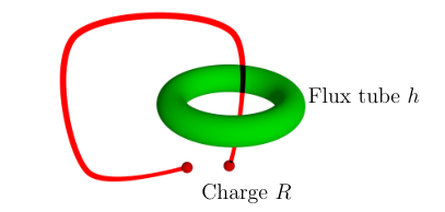
Now that we have discussed what the relevant braiding move is, we need to find how the excitations transform under such a move. The braiding relation is conveniently calculated by considering a commutation of operators as follows. Consider starting with a state that has no excitations and then applying a magnetic membrane operator that produces a flux tube. Then consider acting with an electric string operator to produce a pair of electric charges and move one along the path of the string, with this path passing through the loop excitation. In this case the electric excitation has undergone the braiding move we described earlier. We want to compare this situation to a similar one in which the electric excitation has not braided with the loop excitation. To do so, consider reversing the order of operators that we apply. Instead of first acting with the magnetic membrane and then with the electric string operator, we first apply the electric operator. This produces a pair of electric excitations and moves one of them along the ribbon. However, there is no magnetic excitation present at this stage, so no braiding occurs. Then we act with the magnetic membrane to produce our flux tube. In this situation, the excitations end up in the same location as when we applied the operators in the original order, but no braiding has occurred. Comparing these two situations therefore gives us the braiding relation. This means that to describe the braiding, we just need to find the relationship between the two possible orderings of the operators. That is, we need to calculate the commutation relations of the magnetic membrane operator and the electric ribbon operator.
In the case where is Abelian, it is simple to calculate the commutation relation described above. Let the path of the electric ribbon operator be and consider a magnetic membrane operator applied on a membrane which intersects with the path . The path intersects with the membrane at some edge in . The label of the path up to edge is not affected by the magnetic membrane, because it does not intersect with it. We denote this part of the path by . The path after , which we call , is similarly unaffected. However, the label of the edge itself is multiplied by either or , depending on the relative orientation of the edge and the membrane. Then the total path is the composition of , the edge and , which we write as (if the edge points along the path, otherwise ). This means that the path label operator satisfies the following commutation relation with the magnetic membrane operator:
where the inverse depends on the orientation of the membrane. Because we are looking at the case where is Abelian, we can extract the factor to the front of the path operator and combine the sections of path to obtain
Now consider an electric ribbon operator, which has the form
where is an arbitrary set of coefficients. This ribbon operator then satisfies the commutation relation
| (13) |
with the magnetic membrane operator. This relation is simplified when we consider an electric ribbon operator whose coefficients are described by an irrep of . As discussed in Section III.1, the electric ribbon operators labeled by irreps of form a basis for the space of electric ribbon operators, and so we can decompose any electric ribbon operator into a sum of such irrep-labeled ribbon operators. When is Abelian, all of the irreps are 1D, and so the basis ribbon operator labeled by irrep is given by
where is the representation of element in the irrep, and is a phase because the irreps are 1D when is Abelian. Substituting this into Equation 13, we see that the electric ribbon operator labeled by an irrep and the magnetic membrane operator satisfy the commutation relation
| (14) |
This is the same as the unbraided version , except that we have gained a phase of or . Therefore, under braiding the state obtains a simple phase (or the inverse) and so the braiding is Abelian. The phase is if the electric ribbon’s path meets the direct membrane before the dual membrane, and the inverse otherwise, as we show in Section S-IV.1.1 of the Supplemental Material. Note that this is the same result that we would expect for conventional discrete gauge theory (see, e.g., Refs. Bais 1980; Bucher et al. 1992 and our discussion of how this relates to higher gauge theory in Section II of Ref. Huxford and Simon 2023a).
IV.1.2 Flux-flux braiding
Just as a point particle can be braided with a loop-like excitation in two ways, so can two loops be braided in multiple ways. The allowed patterns of motion can be built from two types of movement. Firstly, we can move the loops around each-other (in the same way as we can move two point particles around each-other), which we call permutation. Secondly, we can pull a loop through another loop (or over it, which is equivalent to pulling the second loop through the first), just as we saw when braiding point particles with loops. These two moves are shown in Figure 15. In this figure, in each case the red loop is moved, with the path of its motion being represented by the yellow membrane. The arrows indicate the direction of motion. In this model, the permutation move is trivial in that it is the same regardless of whether the green loop is present or not. This is because the motion can be performed by membrane operators acting on membranes that never intersect. Then because the membranes do not intersect, the membrane operators commute. Even if we choose to use membrane operators that do intersect, as in Figure 16, the membranes can be deformed so that they do not intersect, by using the topological property of membrane operators. In the example shown in Figure 16, a loop (shown as a small red torus in the figure) is moved along a surface (indicated by the red surface attached to the loop) that intersects twice with a green membrane. Although the red loop intersects the green membrane, the red loop does not pass through the larger green loop excitation created by this green membrane. This motion is performed by an operator placed on the red surface. The red and green membranes can be deformed so that one goes around the other, using the topological property of the membrane operators. Then because the membranes do not intersect (and indeed can be deformed so that they never come close), the corresponding membrane operators commute and so permutation is trivial. This is also true for permutation involving non-confined point particles or the -valued loops: in 3+1d the permutation can be performed by ribbon or membrane operators which do not intersect.


As we did with the flux-charge braiding, we can express the braiding relation between two loops in terms of the commutation relation between creation operators. The flux tubes are created and moved by membrane operators, so the appropriate commutation relation is between two membrane operators, as indicated in Figure 17. In the Abelian case, the two magnetic membrane operators commute, and so the loop braiding between two magnetic fluxes is trivial. This is because in this case, the magnetic membrane operator simply multiplies each cut edge by the label of the magnetic operator. This is in contrast to the non-Abelian case, where the action of the membrane operator on each edge depends on the value of the path from the start-point to that edge. This means that, in the Abelian case, the two membrane operators only share support when their membranes cut some of the same edges, so that the two membrane operators directly change the same edge label. Even then, the action on a shared edge is the same regardless of the order in which the operators act. Consider the action of two membrane operators and on such a shared edge (i.e., one cut by the dual membranes of both operators). If we first act with the membrane operator labeled by and then by the operator labeled by , the edge label goes from to (possibly with inverses on or , depending on the relative orientation of the membranes and the edge). On the other hand, when acts first on the edge, followed by , the total effect on the edge label is given by . This is the same as (because is Abelian), so the two membrane operators commute and the braiding is trivial.
IV.2 Non-Abelian case
IV.2.1 Flux-charge braiding
In the case where is non-Abelian, the braiding relations between the magnetic fluxes and electric charges are a little more complex, although they still match our expectations from conventional gauge theory (see, e.g., Refs. Bais 1980; Bucher et al. 1992 and our discussion in Section II of Ref. Huxford and Simon 2023a). Recall from the Abelian case that the electric string operator fails to commute with the magnetic membrane operator because the latter operator changes the label of one (or possibly more) of the edges along the path of the electric ribbon. In the Abelian case, the action on the path element was simple. The affected edge was multiplied by a fixed element or the inverse, and this factor could be brought to the front of the product of group elements that make up the path element, so that the entire path element was also multiplied by or the inverse. In the non-Abelian case, this is no longer true. Firstly, any changes to the edge cannot simply be extracted to the front of the path element by commutation. Secondly, the action of the membrane on the individual edge that is changed is more complex, depending on the path from the start-point of the magnetic membrane to the affected edge. This means that, rather than multiply the affected edge label by a fixed element , we multiply the label by an element within the conjugacy class of , with this element depending on the path element from the start-point of the membrane to the edge. However, this path element depends on the state that we act on, and even in the ground state the element is not generally fixed (the ground state is made of a superposition of states with different values of this path element) and so we must leave this path element as an operator. Therefore, the braiding relation is not generally well defined. To illustrate this idea, consider performing exactly the same braiding as in the Abelian case, by passing an electric ribbon operator through a magnetic membrane operator. Again we split the path of the electric ribbon into the path before the intersection; the edge along which the ribbon and membrane intersect; and the path after the intersection. Of these parts, only the group element assigned to the edge is affected. For now, assume that the edge points along the path , so that . If this path passes through the direct membrane of the magnetic membrane operator before the dual membrane (i.e., for a particular choice of relative orientation of ribbon and membrane), we have that
where is the path from the start-point of the membrane to the crossing point and we have assumed that the ribbon is aligned so that the path reaches the direct membrane of the magnetic membrane operator before the dual membrane. Then for the entire path element, we have that
If we had taken edge to point against the path, we would have a similar result, because the edge element would appear with an inverse in the path element, but the edge element would be right-multiplied by the inverse factor by the membrane operator, so we would obtain
We can combine these cases by introducing , where is 1 if the edge and path align and otherwise. Then we have
By inserting the identity in the form , we can write the commutation relation as
| (15) |
This is similar to the commutation relation from the Abelian case, except that the path element gains a factor of
instead of simply . This factor is an operator and has no definite value in general, so the effect on the electric excitation depends on which configuration within the ground state we consider and we cannot extract a definite braiding relation. However, there is one special case where we can obtain a definite braiding relation. When the electric string starts at the start-point of the magnetic membrane, then the path sections and start and end at the same points as each-other. Provided that these path sections can be deformed into one-another without crossing over any excitations, the fake-flatness condition imposed by the plaquette energy terms ensures that up to a potential factor of for some . Such factors of do not affect
because is in the centre of , so the factor of and from and cancel. Therefore,
| (16) |
This relation then gives us a simple braiding relation in the “same-site” (or same start-point) case. Note that we gave this braiding relation for a particular choice of relative orientation for the ribbon and membrane operator, and if we reversed this relative orientation then the element would instead be multiplied by (as we show in Section S-IV.1.1 in the Supplemental Material). This braiding relation is a simple extension of the Abelian case. Having said that, the non-Abelian nature of the group does still have some relevance when we use our irrep basis for the electric operators. Recall that the electric excitations are labeled by irreps of the group , combined with matrix indices for the irrep. When is Abelian, these representations are 1D and we need not worry about matrix indices. However, when is non-Abelian some of these irreps are not 1D. We can look at the effect of braiding on an electric ribbon labeled by a representation and its indices, for which we find that:
| (17) |
We see from Equation 17 that the braiding mixes electric ribbon operators labeled by different matrix indices but the same representation. The fact that the representation is left invariant suggests that the representations label the purely electric topological sectors, given that braiding cannot mix different sectors.
The importance of the start-points of the membrane and ribbon operators when it comes to braiding can be interpreted in terms of gauge theory. Just as we discussed for the 2+1d case in Ref. Huxford and Simon 2023b, the start-point of the magnetic membrane can be seen as a unique point in that the flux tube produced by the magnetic membrane operator has a definite flux label with respect to this point even within the conjugacy class. When we give a flux tube a flux label, we must specify the path with respect to which we measure this flux. The path must link with the flux tube, but smoothly deforming the path should not change the flux label measured (where by smoothly deform, we mean pulling through the space represented by the lattice to another position on the lattice). An exception to this is the start-point of the path. Moving this start-point can change the flux label that we would assign to the flux tube (see, e.g., Ref. Alford et al. 1992). Suppose that the flux label measured with respect to a particular start-point is . Then if we measure the flux label of the flux tube starting from a different point, the result is related to by conjugation by a path element for a path between the two start-points. In our model this path element is not usually well-defined, because the energy eigenstates are usually linear combinations of states with different group elements assigned to the path. We say that the path element is generally operator valued. Therefore, the flux tube does not generally have definite flux with respect to points other than the start-point (with an exception if the flux label is in the centre of ). This non-definite flux is reflected in the flux-flux braiding. This idea is explained more clearly in the context of field theory in Ref. Alford et al. 1992.
A second interpretation of the start-point dependent fusion comes from anyon theory. We only have definite fusion in the case where the membrane operators share a start-point. Then, as in the 2+1d case, we may expect that we only have definite braiding when the fusion channel is definite: that is, when the operators involved have a common start-point.
IV.2.2 Flux-flux braiding
As with the flux-charge braiding, the general result of braiding two magnetic fluxes is more complicated when is non-Abelian. However, as with the flux-charge braiding, there is a special case with simple braiding relations, when the two magnetic membrane operators have the same start-point. This makes sense if we think of the base-point as the point of definite flux, because we only expect a definite braiding result if the two flux tubes have definite flux when measured with respect to the same point.
We consider the case where one flux tube (which we will call the inner loop) is passed through another loop (which we call the outer loop). The inner loop takes the role of the red loop in the left diagram of Figure 15. Then in the same start-point case the label of the inner loop is conjugated by the label of the outer loop, while the label of the outer loop is unchanged. That is, if the label of the inner membrane operator is and the outer membrane operator is labeled by , under braiding the label of the excitation from the inner membrane becomes and the label of the outer membrane is unchanged. The simplest way to obtain this braiding relation is to use the topological nature of the operators. We can freely deform the membranes, as long as they do not cross an excitation and no excitations are moved in doing so. We can therefore pull the membrane that produces the inner loop fully through the other membrane (as there are no excitations within the membrane itself). However, when we do this we must keep the start-point fixed (because it may be excited), so the start-point is not moved through the outer membrane. However, recall that the action of the magnetic membrane operator depends on a set of paths from the start-point to the edges being changed by the membrane operator. As we deform the membrane, the start of these paths (the start-point) is fixed, while the ends are pulled through the outer membrane (if these ends were not already on the other side of the membrane). Therefore, all of these paths intersect the outer membrane. This means that the group elements of these paths will be changed by the action of the outer membrane operator, which will in turn affect the action of the inner membrane operator. To see how the inner membrane operator changes under the commutation relation we need to know how the labels of these paths are affected.
As an example, consider Figure 18. In the left side of the figure we have the membranes in their original position, with the red membrane nucleating a loop at the common start-point and moving the red loop through the green one. To calculate the commutation relation, we deform the red membrane so that it is entirely pulled through the green membrane, as in the right side of Figure 18. However, when we deform a membrane we must keep any excitations fixed, including the potentially excited start-point. Therefore, the start-point is fixed. This means that the paths from the start-point to the red membrane, like the example path to the red membrane in the right-hand side of the figure, pass through the green membrane and so can be affected by the green membrane operator. This is significant because these paths determine the action of the membrane operator, as explained in Section III.2. An edge cut by the dual membrane of the magnetic membrane operator has its edge label multiplied by a factor (or the inverse), where is the vertex on the direct membrane that is attached to . These factors have the form , where each path now intersects with the green membrane operator . We must therefore find the commutation relation of such a path label operator with the membrane operator.
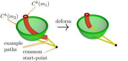
We already saw how a magnetic membrane operator affects the label of paths that pierce the membrane when we looked at the charge flux-braiding. From the charge braiding calculation we know that the label of a path that starts at the common start-point and intersects the outer membrane changes from to , where is the label of the outer membrane operator being intersected (see Equation 16). As discussed previously, this path element appears in the action of the other (inner) membrane operator. If the inner membrane has label , the membrane operator acts on an edge cut by the membrane by multiplying the edge label by , where is the path from the start-point to that edge. Under commutation with the outer membrane, when changes to , this action becomes multiplication by , which is equivalent to the action of an unbraided membrane of label . Therefore, we see that the label of one of the flux tubes is conjugated by braiding. As we expect, the conjugacy class of the flux is invariant under braiding, but the flux element within the conjugacy class can be changed.
It is worth noting that if we had not deformed one membrane to pull it entirely through the other, some of the paths from the start-point would not pierce the other membrane and so would be unaffected by the commutation relation. This means that the action of the membrane in the region from the start-point to the intersection of the membrane is unaltered. This reflects the fact that a membrane operator moves the loop excitation associated to it. Before the intersection, the membrane operator is moving the excitation before it has braided, so its label is the original label of the loop. After the intersection, braiding has occurred and so the label of the membrane (and the excitation) has changed. The precise point at which braiding has occurred is somewhat arbitrary in an anyon theory (although we can guarantee whether braiding has occurred if the excitations start and end in the same position). Similarly the choice of location for the membranes is somewhat arbitrary when the membrane operators act on the ground state because we can deform the membranes without affecting their action, and so we can change the location where the membrane operators intersect by deforming the membranes. This reflects the freedom in considering at which point during the motion the braiding transformation is applied (although if the excitations start and end in the same position, then the membrane operators will definitely intersect if braiding occurs, regardless of how we deform the membranes).
Having obtained the braiding relation, it is useful to consider how braiding affects a linear combination of magnetic membrane operators with label within a certain conjugacy class, such as . If the magnetic membrane operator is an equal superposition of operators labeled by each element of a conjugacy class, then the conjugation of the labels by the braiding only permutes the labels within the conjugacy class, which has no effect when the coefficient for each element is the same. Therefore, the overall membrane operator transforms trivially under braiding. For a general superposition, the conjugation (and so permutation of the labels) does affect the operator and so the braiding is non-trivial. These conditions match the conditions for the start-point of the membrane operator to be unexcited or excited. A magnetic operator with an unexcited start-point is an equal superposition of magnetic operators with labels within a conjugacy class, and so is unaffected by braiding through other magnetic excitations. On the other hand, a magnetic operator with an excited start-point will transform non-trivially when it braids through some other magnetic excitations. This is because, if the start-point is excited, the magnetic excitation carries a point-like charge, which enables it to braid non-trivially with other magnetic excitations when passed through them. Note that the same condition does not hold for the outer membrane operator, which can affect the inner membrane operator even if it does not have an excited start-point. This is because we can shrink the inner loop to a point before braiding it without affecting the braiding relation, whereas the loop-like character of the outer loop is essential for the braiding.
It is important to note that the precise form of the braiding relation depends on the orientation of the loops involved. Flipping a magnetic excitation is equivalent to changing its label from to . Therefore, if we were to flip the orientation of the outer membrane from our earlier calculation, then the label of the inner membrane would change from to under braiding rather than changing to . Flipping the orientation of the inner one does not change the expression, because the transformation is the same when we invert both sides: . Therefore, if the orientation of both loops is flipped, the braiding transformation is
| (18) |
IV.2.3 Linking
In addition to the non-trivial loop-loop braiding, there is another feature of loop excitations not present for point excitations. Two loop excitations may be linked. In this case, depending on the labels of the two excitations, there may be an energetically costly “linking string” that joins the two loops. This situation is indicated in Figure 19. As we show in Section S-IV.1.4 in the Supplemental Material, this linking string is present between two linked magnetic excitations when their labels do not commute. If the two loops are labeled by and and their membranes have the same start-point, then the two loops are linked by a string with a label similar to . The exact label depends on the relative orientations of the two loops and which path we choose to use to define the flux of the linking string (so or could appear with an inverse in the label of the linking string, or the label could be conjugated by or ).

This linking string indicates that there is an obstruction to pushing the two loops through one-another and so pushing them through results in an energetically costly linking string. One way of viewing this is that the two strings are unable to pass through each-other. Therefore, instead of the loops being pushed through each-other, one is deformed to accommodate the other, as shown in Figure 20. In Figure 20, part of one of the loops envelops the other one and folds back on itself, as seen in the bottom-right of the figure (this becomes the pink string in the lower-left of the figure). We can consider this part of the two loops as the linking string. It is possible to work out the flux label of the linking string from this picture by writing a path that links with the thin section as a combination of the paths defining our two original fluxes (recall from Section IV.2.1 that a flux tube is defined along with a path linking with that flux tube, which measures the flux value). A more complete argument for this (in terms of generic fluxes, rather than in terms of this specific model) is given in Ref. Alford et al. 1992.
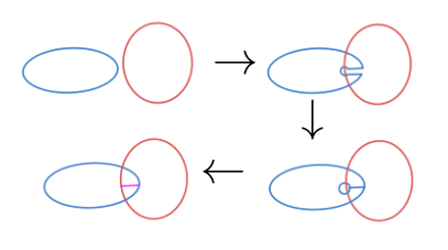
The presence of the linking string indicates that further relative motion of the two loops is non-trivial, because such motion will move the string (the position of which can be detected through the energy terms). For example, we can consider rotating one of the loops by a full rotation. This would be a trivial motion if the loops were unlinked. However, when the loops are linked the linking string will follow this rotation, as shown in Figure 21, indicating that the motion is non-trivial. In order to implement this rotation, we make the direct membrane paths (the paths that we defined when constructing the membrane operator) spiral outwards, wrapping around the linking (blue) loop. If we wanted to write the label of these paths in terms of the label of an unwrapped path, we would gain a factor that accounts for the flux of the blue loop. This in turn affects the action of the membrane operator, changing the effective label of parts of the membrane operator by conjugation by the flux of the blue loop.

IV.2.4 Three-loop braiding
It has become clear Wang and Levin 2014; Jiang et al. 2014 that when considering loops, the simple case where two loops pass through each-other (two-loop braiding, shown in the left side of Figure 15) that we have described so far does not fully describe the general topological properties of loops. A more general example of braiding is where two loops pass through each-other while both loops are linked to a third loop (see Figure 22). This is known as three-loop Wang and Levin 2014 or necklace braiding Bullivant et al. 2020.
In this model however, the result of three-loop braiding is similar to that of the ordinary braiding. The only difference is that the two loops may also drag linking strings with the third loop. This is shown in Figure 22. The transformation of the loop labels is otherwise the same as in the ordinary case. One exception is that the linking string of two magnetic excitations can cancel the confining string of a confined blob excitation (provided that the labels of the linking string and blob excitation agree, as described in Section S-IV.1.4 in the Supplemental Material), which enables those blob excitations to move and braid freely while attached to a linked flux, which they would not normally be able to do.
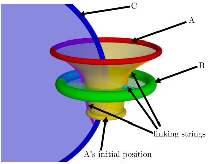
IV.3 Loop-blob braiding
So far we have considered the excitations that are described by the group . The final non-trivial braiding is between the two types of excitation that are associated to the group , the -valued loops and blob excitations. In this case it is easy to find the braiding relations by looking at the effect of the blob ribbon operator on the surface measured by the operator that produces the loop. We consider a situation where the blob excitation passes through the loop excitation. To implement this situation on our lattice, we apply both an -valued membrane operator and a blob ribbon operator whose path intersects with that membrane, as shown in Figure 23.

In order to compute the braiding relation, we compare the situation where we first create the loop and then push the blob through, thus performing the braiding move, with the one where we push the blob through empty space before producing the loop. The relevant commutation relation is shown in Figure 24.
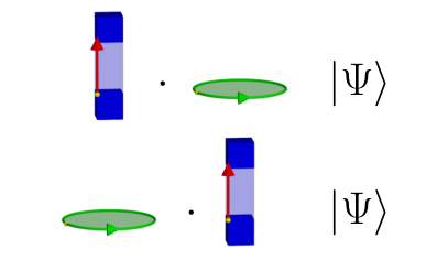
As we saw in Section III.4, the blob ribbon operator with label multiplies the labels of the plaquettes pierced by its path by or , depending on the relative orientation of the plaquette and ribbon. This action is not sensitive to the presence of the -valued loop excitation and so the blob ribbon operator is unaffected by the commutation. On the other hand, the membrane operator for the loop excitation is affected by the action of the blob ribbon operator. Recall that the -valued membrane operator measures the surface element of the membrane on which it is applied. This surface element, , is a product of the elements of individual plaquettes: , where the accounts for the relative orientation of the surface and plaquette. We defined the blob ribbon operator to intersect the membrane, and so it will affect the label of one of the plaquettes in this product. If the blob ribbon operator pierces the membrane through a plaquette , then the label of that plaquette is multiplied by or , depending on the relative orientation of the plaquette and the ribbon. This in turn means that the contribution of the plaquette to the surface will be multiplied by or , depending on the relative orientation of the membrane and the ribbon. The orientation of the membrane matters rather than that of the plaquette, because the in the expression for the surface label accounts for the relative orientation of plaquette and membrane (if the plaquette is anti-aligned with the membrane, the inverse in converts a factor of from the ribbon operator into if the orientation of the ribbon opposes the plaquette but matches the membrane, or vice-versa if the orientation of the ribbon matches the plaquette but opposes the membrane). If the orientation of the membrane matches the orientation of the blob ribbon operator, will be multiplied by . This indicates that in this case. Then, considering the basis operator for our space of -valued membrane operators labeled by an irrep of (as defined in Equation 12), the commutation relation with the blob ribbon operator is given by
where we used the fact that is Abelian to take as a 1D irrep and separate into and . Therefore,
| (19) |
Having the -valued membrane operator on the left of the product (and the blob ribbon operator on the right) corresponds to the unbraided case (because in this case the blob excitation moved before the loop excitation is present), so the braiding of our two excitations results in accumulating a phase of . A similar argument holds in the case where the membrane operator and blob ribbon operator are anti-aligned, except that we should replace by its inverse.
It is worth noting that the blob excitations with label not in the kernel of (that is the confined blob excitations, as we saw in Section III.4) braid non-trivially with the condensed -valued loop excitations (those with trivial representation of the kernel), while those with label in the kernel braid trivially with them. This is because the condensed -valued loop excitations have trivial representation of the kernel: for in the kernel. Therefore, the phase gained is 1 when a condensed loop braids with an unconfined blob (which carries a label in the kernel). This matches our expectation that only the confined excitations can braid non-trivially with the condensed excitations.
IV.4 Summary of braiding when is trivial
For convenience, we summarize the excitations that braid non-trivially with each-other in Table 2. We can see that the excitations split into two sets. The electric and magnetic excitations (the excitations corresponding to the group ) braid non-trivially with each-other and the blob and -valued loop excitations (the excitations corresponding to ) braid non-trivially with each-other, but there is no non-trivial braiding between the two sets.
| Non-Trivial | Magnetic | -valued | ||
| Braiding? | Electric | flux | Blob | loop |
| Electric | ✗ | ✓ | ✗ | ✗ |
| Magnetic | ||||
| flux | ✓ | ✓ | ✗ | ✗ |
| Blob | ✗ | ✗ | ✗ | ✓ |
| -valued | ||||
| loop | ✗ | ✗ | ✓ | ✗ |
V Ribbon and membrane operators in the fake-flat case
Now that we have considered the first of our special cases, where is trivial, we move on to another of our special cases (Case 3). We consider the case where our groups and , as well as our maps and , are completely general, but we restrict our Hilbert space to only allow fake-flat configurations. Many of the features of the excitations are common between the two cases, so we will examine the differences between them rather than repeating our previous discussion entirely.
V.1 Electric excitations
The electric excitations are unchanged by taking non-trivial. Just as in the trivial case, we measure the value of a path and assign a weight according to the value of the path. This creates two point-like excitations at the ends of the path. The operators are best labeled by irreps of the group , with non-trivial irreps giving the excitations and the trivial irrep giving the identity operator. The excitations labeled by irreps with a non-trivial restriction to the image of are confined.
V.2 -valued loop excitations
Next we consider the -valued loop excitations, which are produced by membrane operators that measure the surface label of a membrane:
Here is the surface label of the membrane and the are a general set of coefficients. This operator has the same form as the corresponding operator for the trivial case. However, there is a slight difference when we consider our irrep basis for the space of -valued membrane operators (see Equation 12 for the trivial case). Because our group may now be non-Abelian, the irreps are generally not 1D. This means that our basis for the -valued membrane operators must include the matrix indices for those irreps, so that our general basis operator takes the form
| (20) |
where is an irrep of , and and are the matrix indices.
In addition to this slight difference in the presentation of the basis operators, we also have some physical differences compared to the trivial case. When is non-trivial, whenever we measure a surface we must specify a base-point with respect to which we measure that surface label Bullivant et al. 2017. Because the membrane operator for the -valued loop excitations involves measuring a surface, we must specify a base-point for the measurement. We call that base-point the start-point of our membrane operator. Similarly to the start-point of the magnetic membrane operator, this start-point may be excited by the action of the -valued membrane operator. Recall from Section II that a vertex transform at the base-point of a surface affects the value of that surface, with taking the surface label from to . This means that the vertex term (which is made of a sum of vertex transforms) at the start-point of our membrane operator may not commute with our membrane operator, which may result in the vertex being excited (while the other vertex terms are still left unexcited). Whether the start-point vertex is excited or not depends on whether the coefficients of are a function of the -classes of , where two elements and are in the same -class if there exists a such that (this is an equivalence relation). If the coefficient for each element is equal to the coefficient for each element related by the action, such as , then the start-point is not excited. On the other hand, if for each -class the coefficients for the elements within that -class sum to zero, then the start-point is excited. We note that the irrep basis given in Equation 20 does not provide a good description for this phenomenon, because the coefficients given by the matrix elements of an irrep do not transform in a particular way under an action, and this action can even cause mixing between irreps. Generally, to get membrane operators which either definitely excite the start-point or definitely leave it unexcited, we must consider linear combinations of the basis operators given in Equation 20.
In addition to the start-point, we also need to be careful when determining the boundary of the surface, which supports the loop-like excitation. The boundary of the surface always starts and ends at the start-point of the membrane operator, because this start-point is the base-point of the surface. This means that if we nucleate a loop-like excitation at the start-point and then try to move it away from the start-point, part of the boundary still connects to the start-point, as shown in Figure 25. This section of the boundary is attached to the start-point and the edges in this section appear twice in the boundary, with opposite orientation each time (see Section S-I C in the Supplemental Material of Ref. Huxford and Simon 2023b for more details about the boundary of surfaces), just like a whiskering path of the type considered in Section I D of Ref. Huxford and Simon 2023a (also shown in Figure 4). For this reason, we will refer to such a section of boundary as a whiskered section. As we showed in Section S-I C of the Supplemental Material of Ref. Huxford and Simon 2023b, the edges along such sections of boundary may be excited if is non-Abelian (whereas if is Abelian these edges are never excited). Whether these edges are excited by a particular membrane operator or not depends on the coefficients associated to that membrane operator. For an -valued membrane operator
with a general set of coefficients , the edges on the whiskered section of boundary are left unexcited if the coefficients are a function of conjugacy class, so that for all . For example, if the coefficients are given by the characters of an irrep of (which are invariant under conjugation), then the edges will be unexcited. On the other hand, the edges will be excited if the coefficients within each conjugacy class sum to zero. One important thing to note is that if the start-point is not excited, then the edges from the start-point to the loop are not excited either (as we may expect, because the start-point becomes unimportant when it is unexcited). To see this, we note that if the start-point is unexcited, then the coefficients of the membrane operator are invariant under the action: for all and . In particular, this means that the coefficients are invariant under an action of the form for any : . However, because of the Peiffer condition Equation 2, . That is, the action from an element in is equivalent to conjugation. Therefore, if the coefficient is invariant under any action, it is also invariant under conjugation, and so if the start-point is unexcited then so are any edges on the whiskered section of the boundary.

This idea that there may be a string of excited edges from the start-point to the loop-like excitation is significant for the behaviour of the excitation. If the edges are not excited then it indicates that we can move the loop-like excitation created by the membrane operator without dragging any excitations from the start-point. That is, the excitation is not confined. On the other hand, if the edges are excited then we cannot move the loop-like excitation away from the start-point without incurring an energy cost. This means that the excitation is confined. However, note that the additional energy cost is associated to a confining string which connects the loop to the start-point. This additional energy does not depend on the size of the loop itself. As we discuss in Section IX.1 (although we do not consider the fake-flat case in that section, we would expect a similar result), the loop-like excitations of this model can also carry point-like charge (which is balanced by the charge carried by the start-point). The fact that the confining energy cost depends on the separation of the loop and start-point (rather than the area of the membrane enclosed by the loop) suggests that it is the point-like charge that is confined, rather than the loop-like charge. This is further supported by the fact that the membrane operators that do not produce an excitation at the start-point never produce confined loop-like excitations.
V.3 Blob excitations
The blob excitations are changed significantly by taking non-trivial and enforcing fake-flatness at the level of the Hilbert space. Firstly, as we saw in Section III.4, in the trivial case some of the blob ribbon operators excite the plaquettes along their length (and would still do so when we take to be non-trivial). These confined ribbon operators must be thrown out in the fake-flat case because they violate fake-flatness. This means that the labels of the blob ribbon operators are restricted to lie in the kernel of . Secondly, the action of each blob ribbon operator is more complicated. In addition to the path between the centres of blobs, we must specify a path on the lattice from a privileged vertex, called the start-point of the operator, to the base-points of each affected plaquette. We call this path the direct path, and call the original path (which pierces the affected plaquettes) the dual path. We can either have a single direct path that runs through each of these base-points (so that the path to each base-point is an extension of the path to the previous base-point), or instead have a set of paths, one for each pierced plaquette. Now instead of simply multiplying the plaquette labels by or , the blob ribbon operator left-multiplies the label of each plaquette pierced by the dual path by or right-multiplies the plaquette elements by the inverse, where is the path from the start-point of the ribbon operator to the base-point of the affected plaquette and is the corresponding group element. As in the trivial case, whether the element or its inverse are used depends on the orientation of the plaquette with respect to the dual path of the blob ribbon operator, with the inverse used if the plaquette aligns with the dual path. A simple example of this action is shown in Figure 26.

The way the direct path affects the action of the blob ribbon operator is similar to how the direct path affects the action of the magnetic ribbon in 2+1d (as we saw in Ref. Huxford and Simon 2023b), except that instead of conjugation by the path element we have this action. If we were allowed blob ribbon operators labeled by a general element of (rather than just an element in the kernel of ), the precise path chosen for this direct path would be significant. This is because when we deform a path over a fake-flat surface, while keeping the start and end points fixed, the path label is altered by a factor of the form for some . When is general, this additional factor of causes a non-trivial difference in expressions of the form , such as those which appear in the action of the blob ribbon operator. Specifically, from the Peiffer conditions (Equations 1 and 2 in Section II) we have . However, when we restrict the element labeling the blob ribbon operator to be in the kernel of , we also ensure that is in the centre of the group . To see that elements in the kernel of are also in the centre of , we again use the Peiffer conditions. Given that is an element of the kernel of , the second Peiffer condition (Equation 2) tells us that
That is, elements in the kernel must commute with all elements of . We also note that if is an element of the kernel, then so is for any . This is because , from the first Peiffer condition (Equation 1). Therefore, for any element in the kernel of , is also in the kernel of and so is in the centre of . This means that in our earlier expression, is equal to when is in the kernel, and so the additional factor of from deforming the path is irrelevant, at least when we act on states that obey fake-flatness. Therefore, when we restrict our blob excitations to the non-confined ones, which are labeled by elements of the kernel of , the precise choice of paths from the start-point to the base-points of the affected plaquettes does not matter. This insensitivity to the path is only for smooth deformation over fake-flat regions, so if the lattice supports non-contractible cycles then different choices of path may give different actions for the ribbon operator, with these different actions being equivalent to taking different labels for all or part of the ribbon operator.
Much as we saw with the magnetic excitation in 2+1d, this dependence of the action of the blob ribbon operator on the value of (sections of) the direct path may lead to the blob ribbon operator exciting the start-point of the operator. This is because vertex transforms at the start-point can affect the path label of the direct path. As we show in Section S-I.2.2 of the Supplemental Material, the start-point vertex is not excited if the ribbon operator is an equal superposition of all the ribbon operators labeled by elements in an -class (the sets of elements related by the action), but is excited if the coefficients for the elements in each -class sum to zero.
V.4 Condensation and confinement
In Section III.5, we discussed the pattern of confinement and condensation exhibited by the excitations of the higher lattice gauge theory model when is trivial. In addition, we explained that for any pair of groups and that form a valid crossed module with trivial, there is a family of crossed modules (and so lattice models) differentiated from each-other by different maps (assuming that the two groups can support different homomorphisms ). In each family, the model described by the crossed module for which maps only to the identity of is an “uncondensed model” where there is no condensation or confinement present. Then the transition to other models described by the same groups and (but different ) is a condensation-confinement transition. When is non-trivial, however, the picture is less clear. This is because, given a model described by an arbitrary crossed module, we cannot necessarily construct a corresponding uncondensed model. To see this, consider a generic crossed module . Now suppose that is a non-Abelian group. This means that there are some pairs of elements such that . From the Peiffer condition Equation 2 (see Section II), this means that for this pair. However, there is condensation and confinement when is not the trivial group (as we discussed in the trivial case in Section III.5 and will describe in the fake-flat case later in this section). If there were an “uncondensed” model with , then from the non-Abelian nature of the group implies that . However, this is incompatible with the definition of as a group homomorphism from to endomorphisms on (see Section II), because this definition means that the identity element should be mapped to the identity map on . Therefore, there is no such crossed module and so no “uncondensed” model corresponding to the pair of groups and . Because the Hilbert space is fixed by the lattice and the groups and , for a model described by a general crossed module there does not seem to be a corresponding uncondensed model with the same Hilbert space (at least not in the space of higher lattice gauge theory models, though there may well be another model giving the “uncondensed” phase). This means that we are unable to describe the general model in terms of a condensation-confinement transition in this work. However, we can still describe the pattern of confinement (i.e., which excitations cost energy to separate from their antiparticle) and condensation (i.e., which operators act equivalently to “local” operators on the ground state), which we aim to do briefly in this section.
The first excitations to consider are the electric excitations, some of which are confined due to their ribbon operators exciting the edge terms along the ribbon. These excitations have the same pattern of confinement as in the trivial case considered in Section III.5. Namely, the confined electric ribbon operators have coefficients which satisfy for all and the unconfined ribbon operators have coefficients which satisfy for all and (while general ribbon operators can be split into contributions from the two cases and leave the edges along the ribbon in a superposition of excited and unexcited states).
We next consider the blob excitations. Some of these, namely those created by blob ribbon operators with label outside the kernel of , would be confined, but because the mechanism for this confinement is the violation of the plaquette terms that enforce fake-flatness, these ribbon operators must be excluded from the fake-flat model.
So far, this pattern of confinement is the same as for the trivial case described in Section III.5. However, unlike in that case, some of the -valued loops are also confined, as we described in Section V.2. That is, the -valued membrane operators
whose coefficients are sensitive to conjugation (i.e., does not equal for some pair ) may produce an excited string (in addition to the loop excitation itself) as the loop is moved away from the start-point of the membrane. In particular, if the coefficients satisfy for each , then the string is definitely excited (whereas the string is definitely not excited if for all ). As we noted in Section V.2, this confinement appears to correspond to confinement of the point-like charge carried by the loop excitation, rather than of the loop-like charge, because the confinement energy does not depend on the area of the loop, and the confinement can only occur when the start-point of the membrane is excited (an excited start-point seems to indicate the presence of a non-trivial point-like charge, as we are able to show in Section IX.1.1 for the less general case where maps to the centre of and is Abelian).
Next we consider the pattern of condensation evident in the model in this fake-flat case (Case 3 from Table 1). By this, we mean that we want to look at which excitations can be produced by operators that are local to the excitation itself. That is, condensed point-like excitations can be produced by operators that act only on a few degrees of freedom near the excitations, and condensed loop-like excitations can be produced by operators near the loops (which have linear extent, so the operators need not be local in the traditional sense). Because we are unable to construct the magnetic excitations when we restrict to fake-flatness, the only condensed excitations remaining are -valued loop excitations. Just as in the trivial case, the condensed -valued loop excitations are those that are produced by membrane operators which are not sensitive to surface elements in the kernel of . This is because if the membrane operator is only sensitive to (i.e., is not sensitive to the kernel of ), then it has the same action as an electric ribbon operator measuring the boundary label (whereas a membrane operator sensitive to the kernel of can resolve information not obtainable from the boundary path element).
One interesting fact about this pattern of condensation is that it can coexist with the confinement of the -valued loop excitations. Recall that the condition for the -valued loop excitation to be confined is that for all . This is not mutually exclusive with the condition that the excitation is condensed ( for any and ). For example, consider a crossed module of the form , for which the two groups and are the same, with being the identity map, while maps to conjugation (i.e., ). In this case, the only element of the kernel of is the identity element . Therefore, any -valued membrane operator will satisfy the condensation condition (i.e., any coefficients satisfy for all in the kernel of , because can only be the identity element). This means that any coefficients satisfying the confinement condition for this crossed module will also trivially satisfy the condensation condition. How can it be that an excitation is simultaneously confined and condensed? This is because, as we discussed previously in this section, it is the point-like charge carried by the excitation that is confined. On the other hand, the way we have defined condensation means that the condensation must be of the loop-like charge: we have shown that the loop excitation can be produced by an operator local to the excitation (which has linear extent), but this does not mean that the point-like charge can be produced locally in a point-like sense (i.e., with support only on a few degrees of freedom). This fact demonstrates that in future study of condensation and confinement in 3+1d, we must be careful to consider what exactly we mean by condensation or confinement, and which charges (not just excitations) undergo condensation.
VI Braiding in the fake-flat case
Next we discuss the braiding relations in this special case, Case 3 from Table 1, in which we restrict to fake-flat configurations. The fact that we are unable to include the magnetic excitations (because they violate fake-flatness) means that the braiding relations are rather simple. Indeed, the only remaining non-trivial braiding is between the -valued loop excitations and the blob excitations. Just as in the 2+1d case considered in Ref. Huxford and Simon 2023b, however, the signatures of the magnetic excitations are still present in the ground states of manifolds with non-contractible cycles, which can have labels outside of . Before we discuss the braiding proper, we will briefly describe how the excitations transform as they are moved around such non-contractible cycles.
VI.1 Moving excitations around non-contractible cycles
The first type of excitation that we wish to consider moving around a non-contractible cycle is the electric excitation. The transformation obtained by moving an electric excitation around such a cycle is the same in the 3+1d case as in the 2+1d case considered in Ref. Huxford and Simon 2023b. Namely, if we compare an electric ribbon operator applied on a path to one that is applied on the path obtained by concatenating the original path with a non-contractible closed path is
| (21) |
where is the electric ribbon operator labeled by irrep of and matrix indices and . We see that there is mixing between different electric ribbon operators labeled by the same irrep , with this mixing controlled by the matrix representing the path element in irrep . The path element is an operator, and the ground states are not typically eigenstates of this operator even for closed paths .

In a similar way, we can find how the -valued loop-like excitations transform as they are moved around a non-contractible cycle. In order to do so, we compare -valued membrane operators applied on two membranes and which are the same except that is whiskered around the non-contractible cycle . This is because the membrane operators are topological, and so a membrane travelling around the cycle can be deformed by shrinking the section of the membrane around the cycle down to nothing, so that only a whiskering path remains, as shown in Figure 27. Then the -valued membrane operator applied on this whiskered membrane is given by
where is the irrep of labeling the membrane operator (and and are the matrix indices labeling the operator). The surface element can be written in terms of the surface element of the unwhiskered membrane using the rules for whiskering surfaces given in Ref. Bullivant et al. 2017. We have
where is the closed cycle, which is also the path between the start-points of the two membranes. Then we have
| (22) |
The matrix can be considered as the matrix representation for element in a new irrep, . Therefore, we see that moving the -valued loop excitation around the path mixes the irreps related by this action. We say that irreps related by the action of for some belong to the same -Rep class of irreps.
The final type of excitation to consider passing around a non-contractible cycle is the blob excitation. Recall from Section V.3 that the action of a blob ribbon operator on a plaquette pierced by the ribbon is (choosing the plaquette to be aligned with for simplicity)
Taking the path to be , where is a closed non-contractible cycle, we can write this action as
which is the same as the action of a blob ribbon operator that does not wrap around the cycle (so that the path is just ) except with replaced by . Note that here we have taken the direct path of the ribbon operator to wrap around the non-contractible cycle, but not the dual path. If we also let the dual path wrap around the cycle then the plaquettes pierced by obtain two factors acting on the plaquette label, one from the ribbon before it wraps the cycle (corresponding to the label ) and one from the ribbon after it wraps the cycle (corresponding to the label as above).
VI.2 Loop-blob braiding
Compared to the loop-blob braiding that we saw in Section IV.3, the loop-blob braiding in this special case is slightly more complicated. This is because the action of the ribbon and membrane operators involved now depends on the values of various paths on the lattice. For example, as we saw in Section V.3, the blob ribbon operator multiplies plaquette elements by a group element which depends on the label of a path. This label is really an operator, because the value of the path label depends on what state we are acting on. In particular, the ground state does not have a definite value of this label, instead being made up of a linear combination of states with different path labels. Because of this, we may expect that the braiding does not generally give us a definite result and that the braiding relation may depend on such operator-valued labels. However, as with the braiding of the flux tubes that we saw in Section IV.2.2, the braiding relations are simple for particular cases where the start-points of the operators match. Therefore, we are most interested in these same start-point commutation relations. To understand these, it will be useful to first discuss the interpretation of the blob and loop excitations in 2-gauge theory.
Similar to lattice gauge theory, it is useful to consider the gauge invariants of higher lattice gauge theory, which can be built from quantities associated to closed loops and surfaces Bullivant et al. 2017. In addition to the “1-flux” of loops, which is also present in ordinary gauge theory, we have the “2-flux” or 2-holonomy of closed surfaces. The 2-flux itself, described by an element of , is not a gauge-invariant quantity. However, the 2-flux of a closed surface is only changed within certain equivalence classes of elements by the gauge transforms Bullivant et al. 2017 (as we will see for tori and spheres in Sections S-V.2 and S-V.4 in the Supplemental Material), and so these classes in are gauge-invariant, with the identity element in particular belonging to a class of its own. This means that the 2-flux is still a useful quantity. In this model, the blob excitations are associated to non-trivial 2-flux on a surface enclosing the blob excitation. The boundary of the excited blob is itself a surface with non-trivial 2-flux, because an excited blob by definition has a non-trivial surface label on its boundary. To measure this 2-flux, we must pass a loop over the closed surface whose 2-flux we wish to measure. When we measure the 2-flux, we must specify the base-point with respect to which we measure the 2-flux. The choice of base-point is equivalent to a gauge choice, so choosing a different base-point can give a different element for the 2-flux, within the same -class (i.e., the new element is related to the old one by a action). Once we have chosen the base-point, our measurement loop must be nucleated at that base-point before being passed over the surface, as shown in Figure 28. In this model, the -valued loop excitations measure 2-flux, as we can see from the fact that the corresponding measurement operators assign a weight to each possible surface label.

This idea about measuring a 2-flux has important ramifications for our braiding. We have seen that the blob excitations are non-trivial 2-fluxes and the -valued loop excitations measure surface elements, so these loop excitations can measure the 2-flux of the blob excitations. This is why there is non-trivial braiding between these two types of excitation. When we compare the situation where the loop excitation is passed over the blob to the situation where it is not (i.e., we compare the braided case to the unbraided case), we measure the 2-flux of the blob excitation. However, the blob ribbon operator produces excitations that have definite 2-flux only with respect to the start-point of the blob ribbon operator. Similarly, the -valued loop measures 2-flux with respect to the start-point of the membrane operator that creates the loop excitation. Therefore, we expect a definite braiding relation when the start-point for our blob ribbon operator matches the start-point for our -valued loop membrane operator. Note that when is trivial, the start-points lose meaning (we do not need a direct path for the blob ribbon operators and the surface does not need a base-point for the -valued loop) and the loop can be nucleated at any point before being passed over the blob excitation (rather than at the specified start-point of the blob ribbon operator). This is why the braiding is simple when is trivial (as discussed in Section IV.3) and it is not necessary to fix the positions of the start-points in that case.
While we have discussed braiding of the blobs and the loops so far in terms of passing the loop over the blob, we can equally move the blob excitation through the loop instead. These are equivalent, but it is slightly easier to calculate the latter situation. The relevant commutation relation to calculate this braiding relation is shown in Figure 24. Again, we must ensure that the start-points of each operator are in the same location.
The result of this same-site braiding, where we pass a ribbon operator through an -valued membrane operator , is then
as illustrated in Figure 29 (and proven in Section S-IV.2 in the Supplemental Material). The operators for each label form a basis for our space of -valued membrane operators, but we want to consider the commutation of one of the basis operators labeled by an irrep of instead. We have that
| (23) |
If is a 1D representation the braiding therefore results in the accumulation of a phase of . If is higher-dimensional, then it would seem that there is mixing between the different matrix indices. However, recall from Section V.3 that in order to ensure fake-flatness we restricted the label of the blob ribbon operators to be in the kernel of and therefore the centre of . The matrix representation of an element of the centre is a scalar multiple of the identity from Schur’s Lemma, so we can write (where the index could be replaced with any index). This means that the braiding relation 23 simplifies to
| (24) |
so again we only accumulate a phase (this matrix element must be a phase because the matrix is diagonal and unitary, and in fact the matrix element can be used to define an irrep of the kernel of ).
We see that the braiding relation between the -valued loops and blob excitations is similar to the result we found for the braiding of magnetic fluxes and charges that we discussed in Section IV.2.1, except that in this case the irrep labels the loop-like, rather than point-like, excitation.
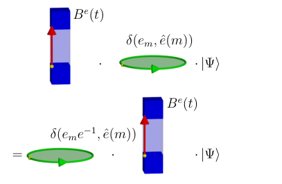
VI.3 Summary of braiding in the fake-flat case
In Table 3, we summarize the braiding in the fake-flat case by indicating which excitations can braid non-trivially. Note that when we enforce fake-flatness on the level of the Hilbert space, there are no magnetic excitations, although we can still have non-trivial flux labels around non-contractible loops on manifolds that are not simply connected (e.g., the 3-torus).
| Non-Trivial | -valued | Around | ||
| Braiding? | Electric | Blob | loop | handle |
| Electric | ✗ | ✗ | ✗ | ✓ |
| Blob | ✗ | ✗ | ✓ | ✓ |
| -valued | ||||
| loop | ✗ | ✓ | ✗ | ✓ |
VII Ribbon and membrane operators in the case where centre() and is Abelian
So far, we have examined the excitations of the higher lattice gauge theory model in two cases. Firstly, we looked at the case where is trivial, where we can find all of the excitations of the model. However, in this case the membrane operators corresponding to the 2-gauge field (labeled by the group ) are simple, and produce no excitations at the start-point of the corresponding operators. Secondly, we looked at the case where is general, but where we restrict our Hilbert space to the fake-flat subspace, thus having to exclude the magnetic excitations. This gave us more interesting excitations from our 2-gauge field, allowing the -valued membrane operators and blob ribbon operators to produce additional excitations at the start-points of the operators. However, excluding the magnetic excitations removes the interesting features from the 1-gauge field excitations. In the following sections, we consider a generalization of the trivial case, which will allow us to keep all of the excitations while also gaining many of the features from the general case. This means that we will be able to see how the magnetic excitation interacts with the more general 2-gauge excitations. We consider the case where is Abelian and maps onto the centre of (Case 2 in Table 1). Note that this case includes the trivial case as a sub-case, so this is a strict generalization of the situation considered in Sections III and IV.
In this case, many of the features of the general crossed module (but fake-flat) case are preserved, despite our restrictions on the crossed module. The electric, -valued loop and blob excitation creation operators are all the same as in the general crossed module (but fake-flat) case (see Section V), except that we also allow blob ribbon operators with labels outside the kernel of and the irreps that label the basis -valued membrane operators are 1D. Because of this, we will not describe the operators that produce these excitations again. On the other hand, we can include excitations analogous to the magnetic excitations from the trivial case. The membrane operators that produce these magnetic excitations are significantly altered from the trivial case that we considered in Section III.2, however. This alteration of the membrane operators is necessary to ensure that each membrane operator commutes with the various energy terms, apart from those near the boundary of the membrane. The magnetic membrane operators affect the edge labels in the same way as in the trivial case, but they also affect the plaquette labels near the membrane. Recall that to specify our magnetic membrane we had to define a dual membrane, with the operator changing the labels of the edges cut by the dual membrane, and a direct membrane, with paths on the direct membrane controlling how the cut edges were changed (see Figure 7). As well as edges, the dual membrane cuts through the plaquettes between these edges (such as the vertical plaquettes in Figure 30). In this new case, the magnetic membrane operator changes the label of the “cut” plaquettes if their base-points lie on the direct membrane. We say that plaquettes whose base-points lie on the direct membrane are based on the direct membrane. The action of the operator on these plaquettes depends on paths on the direct lattice, in a similar way to the action on the edges. Given a cut plaquette based on the direct membrane, the action of the membrane operator on the plaquette depends on the label of a path from the start-point of the membrane to the base-point of the plaquette. An example of this type of path is shown in Figure 30. We denote the group element assigned to the path between the start-point and the base-point of plaquette by , where is the privileged start-point of the membrane operator and is the base-point of the plaquette . If is cut by the dual membrane and based on the direct membrane, then its label is changed from to . As we mentioned previously, the magnetic membrane operator only acts on a cut plaquette in this way if the plaquette is based on the direct membrane. That is, if the plaquette has its base-point away from the direct membrane, then the label of the plaquette is not affected by this action. It may seem arbitrary that the plaquette label is only changed in this way if its base-point is on the direct membrane. However, this is analogous to the action of vertex transforms, which only affect plaquettes that are based at the vertex on which we apply the transform (except instead of only affecting surfaces based at the vertex, the membrane operator affects surfaces based on that surface). Indeed, we demonstrate that closed magnetic membrane operators are closely related to the vertex transforms in Sections S-II.4 and S-II.5 of the Supplemental Material.

The action on the plaquettes is not the only additional feature to the magnetic membrane operator in this new special case. Changing some of the edge labels by multiplication and plaquette labels by this action leaves the blob conditions for blobs cut by the dual membrane unsatisfied (recall that the blob condition enforces that the total surface label of the blob is trivial). To correct this and ensure that the membrane operator commutes with the blob energy terms near the bulk of the membrane, blob ribbon operators (of the type considered in Section V.3) are added to the membrane operator. For every plaquette that is entirely on the direct membrane (not cut by the dual membrane, but instead lying flat on the direct membrane), we have one such blob ribbon operator associated to that plaquette. We call the associated plaquette the base plaquette for that blob ribbon operator. The blob ribbon operators all start at the same privileged blob, which we call blob 0 and must define when specifying the magnetic membrane operator. The blob ribbon operators end at the blob that is connected to the base plaquette and cut by the dual membrane, as shown in Figure 31. The label of this blob ribbon operator, for a base plaquette on the direct membrane and with orientation away from the dual membrane (downwards in Figure 31, as shown in Figure 32), is given by , where is the label of the base plaquette and is the base-point of the plaquette. If the plaquette has the opposite orientation, we must invert the label in this expression. After incorporating this additional action for the magnetic membrane operator, we write the total magnetic membrane operator (denoted by , where indicates that it is the total operator) as
| (25) |
where blob is the blob attached to base plaquette and cut by the dual membrane (note, however, that the same blob may be attached to multiple base plaquettes). In Equation 25, performs the action of the membrane operator on the edges and the action on the plaquettes, while the operators are the added blob ribbon operators (see Section V.3 for a description of blob ribbon operators).


Even with these modifications, the magnetic membrane operator still excites more energy terms than in the trivial case (i.e., more than just the boundary plaquettes and potentially the start-point vertex). Firstly, the privileged blob, blob 0, is not generally left in an energy eigenstate. This is because the blob ribbon operators that we added to the magnetic membrane all originate in this blob and so change the surface label of the blob, from in the ground state to , where is the total surface label of the direct membrane. is an operator, which means that blob 0 is not generally left in an energy eigenstate. Secondly, the edges around the boundary of the direct membrane are potentially excited. This is because the labels of the added blob ribbon operators depend on the labels of the plaquettes on our direct membrane. Edges in the bulk of the membrane are attached to two plaquettes on the membrane and so the edge transform affects the blob ribbon operators associated with both plaquettes. These effects on the labels of the two ribbon operators (together with a contribution from the edge transform on the plaquettes cut by the dual membrane) cancel out, so that the edge transform commutes with the membrane operator, as we show in Section S-I.4.3. On the other hand, edges on the boundary of the membrane are only attached to one plaquette on the membrane, so there is no such cancellation. These boundary edges are therefore not generally left in an energy eigenstate.
VII.1 Condensation and confinement
In the previously considered trivial (see Section III.5) and fake-flat cases (see Section V), we saw that many of the excitations are confined, meaning that it costs energy to separate a pair of excitations, in addition to the energy required to produce the pair. We also found that other particle types are condensed, meaning that they can be produced by local operators (local to the excitation, in the sense discussed in Section III.5) and so carry trivial topological charge. The pattern of condensation and confinement in the Centre() case is the same as in the trivial case discussed in Section III.5. The blob excitations with label not in the kernel of are confined, as are the electric excitations labeled by irreps of that have non-trivial restriction to the subgroup of . On the other hand, the condensed excitations are the magnetic excitations with label in the image of and the -valued loops that are labeled by irreps of which are trivial on the kernel of . These properties, along with the other properties of the excitations in this case, are summarised in Figure 33.
VIII Braiding in the case where centre() and is Abelian
Now that we have described the membrane and ribbon operators that produce our excitations, we can consider the braiding relations of these excitations. Any braiding not involving the magnetic excitations is the same as in the fake-flat case described in Section VI. Namely, there is non-trivial braiding between the blob excitations and the -valued loops, with the same start-point braiding resulting in an accumulation of phase. The result is a phase, rather than the more general transformation given in Equation 23 for the case considered in Section VI.2, because the irreps of are 1D when is Abelian.
Unlike for the fake-flat case, we can find the magnetic excitations and so describe their braiding relations. However, rather than using the magnetic membrane operator directly, it is convenient when considering braiding to combine the magnetic membrane operator with an -valued membrane operator. We multiply the magnetic membrane operator by an -valued membrane operator such as , acting before the magnetic membrane operator. That is, we construct membrane operators of the form , which we denote by . We note that combining the magnetic membrane operator with this -valued membrane operator in this way does not excite regions of the lattice not already excited by the magnetic membrane operator, because both membrane operators only cause excitations near the boundary of the membrane, and possibly at blob 0 and the start-point of the membrane. We will shortly explain why we perform this combination of membrane operators (in essence, it gives the loop-like excitation a well-defined 2-flux), but before we discuss this we shall consider the combination of the membrane operators in more detail.
In order to combine the magnetic and -valued membrane operators, there are some details that we must specify. The first of these is the relative orientation of the two membrane operators. We take the orientation of the -valued membrane operator to point away from the dual membrane of the magnetic membrane operator. The second detail is more subtle. In addition to combining this -valued membrane operator with the magnetic membrane operator, we move blob 0 and the start-point of the membrane operator so that they are displaced slightly away from the membrane itself, as shown in Figure 34. We do this because the -valued membrane may cause an excitation at the start-point, which would prevent us from using the topological nature of the magnetic membrane operator to deform the membrane. It is not necessary to move blob 0 in this way, but it will be convenient when considering topological charge to have a clear separation between the point-like excitations (blob 0 and the start-point) and the loop-like excitation at the boundary of the membrane. A third detail is our convention for the overall orientation of the total membrane operator. Because we have displaced the start-point away from the membrane in a particular direction, it is sensible to define the orientation of the membrane to be consistent with this displacement. That is we imagine that the loop excitation is nucleated at the start-point and moves away from the start-point along the membrane. Therefore, the loop excitation would be oriented downwards in Figure 34, matching the orientation of the -valued membrane operator.

Having considered these details about the combined membrane operator, we now explain why this combination was useful. As we mentioned in Section VII, the action of the magnetic membrane operator generally causes the privileged blob, blob 0, of the membrane to acquire a non-trivial 2-flux (non-trivial surface label). However, this surface label is given in terms of an operator (the surface label of the membrane itself) and so is not well-defined. Including the -valued membrane operator ensures that the 2-flux of the privileged blob 0 after the action of the magnetic membrane operator is well-defined. Giving blob 0 a definite 2-flux is significant because we expect the loop-like excitation to also carry a non-trivial 2-flux to balance the 2-flux of blob 0, and we expect the value of this 2-flux to be important in braiding relations. As we show in Section S-IV.3 of the Supplemental Material, the surface label of blob 0 after the action of the combined membrane operator (with displaced start-point, which does affect the label) is given by . As we show in Section S-IV.3 (see Equation S105), the 2-flux of the loop excitation labeled by and is given by
| (26) |
which is the inverse of the 2-flux carried by blob 0. Due to the fact that the excitations produced by this combined membrane operator carry both ordinary magnetic flux and this 2-flux, we call the combined membrane operator a “higher-flux membrane operator” and call the excitations higher-flux excitations. If we wish to instead consider the original magnetic membrane operator (without the attached -valued membrane operator), we can simply sum over each value of , because this gives us a complete sum of projectors . That is and so
| (27) |
Having constructed this higher-flux membrane operator, we can now use it to find the braiding relations involving the higher-flux excitations. Because the action of the higher-flux membrane operator on the edges is the same as that of the magnetic membrane operator from the trivial case, the braiding relation between the magnetic and electric excitations is the same as in that case (which is described in Section IV). However, as we will see shortly, the braiding between the higher-flux loop excitation and the other excitations is significantly altered. In particular, because the higher-flux excitations can carry a non-trivial 2-flux, we expect non-trivial braiding relations with the -valued loops, which measure 2-flux.
VIII.1 Braiding of the higher-flux excitations with blob excitations
The first braiding relation we examine is between the higher-flux excitations and the blob excitations. We consider a blob ribbon operator , applied on a ribbon , piercing the membrane of a higher-flux membrane operator , applied on a membrane . The ribbon intersects the membrane at a plaquette , as shown in Figure 35. Note that the orientation of the operators is significant. We first look at the case where the blob ribbon operator pierces the direct membrane of the magnetic membrane operator before the dual membrane. If the membrane is oriented downwards, as in Figure 35 (note that the point-like excitation is above the loop) then the ribbon is oriented upwards (at the point of intersection at least).

We have seen in previous cases that braiding is frequently well defined only when the start-points of the membrane and ribbon operators match. However, we shall first examine the general case where the start-points are arbitrary. As usual, we can relate the braiding relation to a commutation relation between the two operators. We compare the case where the magnetic membrane is produced first, and then the blob excitation moved through it, to the reverse case. We find that, as demonstrated in Section S-IV.3.1 in the Supplemental Material,
| (28) |
In this expression, we note that the original ribbon operator is split into two parts, on ribbons and , which transform differently under the braiding. Here starts at the original origin of ribbon and ends at blob 0 of the membrane (corresponding to the part of the ribbon before the intersection with the membrane, except that it is diverted to end at blob 0 of ), while starts at blob 0 and ends at the original end of ribbon (corresponding to the part of the ribbon after the intersection), as shown in Figure 36. We therefore see that, under commutation, the ribbon is diverted to pass through blob 0 of the membrane, and after passing through this blob it changes label from to .

The fact that the label of the blob ribbon operator before the intersection is unaffected by the commutation relation is perhaps unsurprising, because this part of the operator corresponds to the motion of the blob excitation before it braids with the magnetic excitation and so before it has undergone its transformation. This can be seen from the fact that the blob ribbon operator actually creates two excitations and the one which is not moved should not be affected by the other one moving through the loop excitation. Another thing to note is that, as long as the blob ribbon operator is not confined, we can deform the ribbons of the blob ribbon operators without changing their action, as long as we keep the end-points fixed. Because of this, it doesn’t matter at which plaquette our magnetic membrane and blob ribbon operators intersect.
In addition to the transformation undergone by the blob ribbon operator, the label of the higher-flux excitation changes from to . This transformation of the -label of the membrane operator is simply the standard braiding relation between a blob excitation and an -valued membrane, as we saw in Section VI. We note that this result and the other results given in this section, are proven fully in Section S-IV.3.1 in the Supplemental Material.
If we give the magnetic membrane operator and the blob ribbon operator the same start-point, the braiding relation that we explained above simplifies and we are able to remove the operator from the relation. We move the start-points together, without moving them through the higher-flux membrane (which would alter the commutation relations found so far). In this case the blob label goes from before the braiding to afterwards (at least in the part after the intersection) and the label of the higher-flux membrane operator goes from beforehand to . If we had used the opposite orientation, obtained by reversing the direction of the blob ribbon operator, instead the blob label becomes and the membrane label becomes . Again, this result is proven in Section S-IV.3.1 of the Supplemental Material.
If we want to consider the braiding of the original magnetic excitation, produced by the membrane operator , we simply need to sum over the -valued label of the higher-flux membrane operator. Then we have, from Equation 28
| (29) |
from which we see that the magnetic excitation is unchanged by the braiding, whereas the blob excitation is affected in the same way as in the braiding with the higher-flux excitation.
VIII.2 Braiding with other higher-flux excitations
Next, we consider the braiding between two higher-flux excitations. As we described in Section IV.1.2, there are two kinds of braiding for loops. The first, which we call permutation, involves moving two loops around each-other without passing through one another. The other, which we term braiding, involves passing one though the other. As we discussed in Section IV.1.2, the permutation move is trivial in this model. Therefore, we just consider the braiding move. In this motion, shown in Figure 37, one of the magnetic loop excitations (indicated by a small red ring) is moved along the red surface and through another loop (indicated by a large green loop attached to a large green surface). To calculate the braiding relation we apply membrane operators on these surfaces and examine the commutation relations between the membrane operators.

We define the membrane operators as indicated in Figure 37, but then we use the topological nature of the magnetic membrane operators to pull through (as we did in the trivial case in Section IV.2.2), while keeping the start-point and blob 0 fixed. In Section S-IV.3.2 in the Supplemental Material, we show that this leads to the commutation relation
| (30) |
where is the path element for the path between the two start-points of the membranes and
| (31) |
To simplify the expression, we used to denote the label of the plaquette when we move its base-point to the start-point of . This quantity is equivalent to . Furthermore, we used to denote a blob ribbon operator that runs from blob 0 of to blob 0 of and to denote a blob ribbon operator running from blob 0 of to the blob on that is attached to plaquette . These blob ribbon operators may seem complicated, but the situation is analogous to the braiding of blob ribbon operators with the magnetic membranes. Each of the blob ribbon operators that we added to the magnetic membrane operator has a similar commutation relation with the magnetic membrane operator as an ordinary blob ribbon operator. Namely, the blob ribbon operator splits into two parts, one that runs from blob 0 of to blob 0 of and one which runs from blob 0 of to the final destination of the original blob ribbon operator. The only difference from the ordinary blob ribbon operator braiding is that the label of the blob ribbon operator is an operator (depending on the label of a plaquette on ), which causes an additional apparent change to the label even for the part of the blob ribbon operator before the intersection. However, this does not reflect a real change to the blob ribbon operators before the intersection. This is because we can combine the blob ribbon operators that pass from blob 0 of to blob 0 of into a single blob ribbon operator, and use to fix its label in terms of instead of an operator. As shown in Section S-IV.3.2 in the Supplemental Material, this gives us
| (32) |
Now the section of blob ribbon operator between blob 0 of each membrane, which is the part of the ribbon operator before the intersection of the membranes, is labeled by . This is the same label as it would have if we combined the blob ribbons on these sections in the absence of the second higher flux membrane . That is, this part of the blob ribbon operator is unaffected by the braiding, as we may expect given that this section of ribbon operator is the part before the intersection of the membranes. We can contrast this with the sections of the blob ribbon operators after the intersection (which should be affected by the braiding) which have their labels changed from
to
We see that the only change is that we replace with . This matches how the label of the higher-flux membrane operator transforms under braiding (as we see from the operator in Equation 32). That is, the labels of the blob ribbon operators after the intersection (i.e., after braiding) are the labels we expect given the label of the magnetic part of the membrane operator after intersection.
Apart from this splitting of the blob ribbon operators at the intersection of the membranes, we see that the labels of the two membrane operators change (as we mentioned previously for ). We have that
As usual for our braiding, when the start-points of the operators are not the same, we have operators in our braiding relations. When we take the start-points to be the same, these relations simplify to
| (33) |
This removes any operators from the labels, so that we have definite braiding. Note that the transformation of the 1-flux labels ( and ) is the same as for the braiding of two magnetic excitations in the -trivial case, as given in Equation 18 in Section IV.2.2, replacing with (that equation in particular because we used the specific orientation of the loops also used to find that equation). However, the expression for the change of the labels is not so easy to interpret. It is easier to understand these results if we change variables, from the surface labels of the membranes to the 2-fluxes possessed by the loop-like excitations, as we discussed at the start of Section VIII. The 2-flux of the loop excitation, , is related to the -flux label, , and the surface label of the membrane operator by . Therefore, we define
Then, from our braiding relations in Eqs. 33, under braiding these 2-fluxes transform according to
| (34) |
This means that the product of the two fluxes transforms as
under the braiding, which indicates that the product of these 2-fluxes is conserved.
Putting this together, we can see that the 1-fluxes and 2-fluxes of the loop-like excitations transform as
under braiding, where the fact that one loop is moved past the other during the braiding is represented by swapping the order of their labels in the brackets.
We also wish to work out the inverse transformation, which describes the reversed braiding process. Denoting the result of the forwards transformations as primed versions, we have from Eqs. 34:
The inverse transformation is therefore
| (35) |
This matches the braiding proposed in Ref. Bullivant et al. 2019 for higher gauge theory based on discussions of the loop braid group. It is important to note that the braiding depends on the result of fusing the two excitations. Given two loops with 1-flux and 2-flux given by for the first loop and for the second loop, there are many possible fusion products. The fact that the products of 1-fluxes (swapping the order after braiding to account for the swapping of loop positions) and of 2-fluxes are conserved indicates that these are the total 1-flux and 2-flux of the combined loops, and so we have obtained the braiding when they fuse to give the labels . We could equally have considered the braiding in a different situation, such as when the start-points of the two operators are in different positions, for which the loops and fuse to give different total quantum numbers than .
As we did when considering the braiding of the higher-flux with the blob excitation, we can also consider the braiding of our original magnetic excitation, before we pinned an additional -valued loop to it. As described by Equation 27, we can obtain the original magnetic membrane operators from the higher-flux membrane operators by summing over all possible elements of for the label. That is, we consider
Using Equation 30, we see that this gives us
Then we have
because summing over gives us an equal sum over all Kronecker deltas , regardless of the actual value of . This gives us
We can similarly use the sum over to remove the other Kronecker delta. We have
because runs over all . This gives us the final result
| (36) |
Then looking at the effect of braiding on the -valued label, we see that the result is simply conjugation of one of the magnetic flux labels by the other. The labels of the blob ribbons corresponding to are also changed before and after the intersection of the two membranes. Just as we discussed for the higher-flux membrane operators earlier in this section, the label after the intersection reflects the change to the label of the membrane operator applied on , while the change to the label before the intersection is only an apparent change due to the operator label.
VIII.3 Braiding with -valued loops
The final braiding relation to consider is the braiding between these higher-flux excitations and the -valued loops. We can obtain this relation from the calculation for two higher-flux membrane operators in the previous section, because the -valued loops are simply higher-flux excitations with trivial -label. We therefore simply need to take the special case of that calculation when one of the elements is . Rather than repeating the full equations, we will only present the results in the same-start-point braiding case.
First we consider the case where the red excitation shown in Figure 37 is a higher-flux excitation, produced by a membrane operator , while the green excitation is a pure -valued loop, labeled by . In this case the label of the -valued loop transforms as under the braiding, while the labels of the magnetic membrane operator are unaffected by the braiding. When we change to consider our irrep basis for the -valued loops (given in Equation 12) this transformation gives us a phase of
| (37) |
where is the irrep of labeling the -valued loop. Note that if we consider the ordinary magnetic excitation by averaging over , the braiding relation is different for each value of , so the different terms in the sum accumulate different transformations. This is part of the reason why it was necessary to consider the higher-flux membrane instead of the magnetic one in the first place. The result of this different transformation for the different -labels is that, even if the excitation is initially an ordinary magnetic excitation, with an equal superposition of the different -labels, it will not necessarily remain so after braiding, instead becoming an uneven superposition of the different higher-flux excitations, with labels coupled to the state of the -valued loop.
Now we consider the opposite case where the -valued loop passes through the magnetic one. In this case, the red excitation from Figure 37 is a pure -valued loop excitation produced by the membrane operator , while the green excitation is a higher-flux loop excitation produced by the membrane operator . In this case the label of the -valued loop transforms as under the braiding, while the labels of the higher-flux operator are again unaffected by the braiding move. In our irrep basis for the -valued membrane operators, this transformation actually changes the irrep labeling the membrane operator to a different irrep in the same -Rep class of irreps (where two irreps of , and , are in the same -Rep class if there exists a such that for all ). This suggests that the irreps of are not by themselves good labels for the topological charge, because the irreps are not invariant under braiding, and instead the -Rep classes should be important (although the condensation further affects the topological charge). However, as we see in Section IX.1.1, the point-like charge of the loop-like excitations actually depends on how the coefficients of the membrane operator transforms under the action, and so this topological charge has some dependence on quantities within the class as well. We will discuss the topological charge in more detail in Section IX.
VIII.4 Summary of braiding in this case
Table 4 summarizes which types of excitation can have non-trivial braiding relations in the case where is Abelian and maps to the centre of , where non-trivial braiding between the types of excitation is indicated by ticks. Note that the higher-flux excitations have potentially non-trivial braiding relations with every class of excitation.
| Non-Trivial | Higher- | -valued | ||
| Braiding? | Electric | flux | Blob | loop |
| Electric | ✗ | ✓ | ✗ | ✗ |
| Higher- | ||||
| flux | ✓ | ✓ | ✓ | ✓ |
| Blob | ✗ | ✓ | ✗ | ✓ |
| -valued | ||||
| loop | ✗ | ✓ | ✓ | ✗ |
IX Topological charge
In Ref. Huxford and Simon 2023a we explained the concept of topological charge and in Ref. Huxford and Simon 2023b we presented a detailed construction of the measurement operators for topological charge in the 2+1d case. To briefly restate our explanation from Ref. Huxford and Simon 2023a, topological charge is a quantity that is conserved, so that the only way to change the topological charge in a region is to apply an operator that connects this region to the rest of our lattice. Further conditions are imposed on the topological charge relevant to our model by requiring that the ground state is the topological vacuum. There is a significant difference between the 2+1d and 3+1d cases, however. Whereas we consider the topological charge in regions isomorphic to disks (or unions and differences of disks, like annuli) when there are only two spatial dimensions, there are more topologically distinct regions to consider when there are three spatial dimensions. For example, we have both topological balls and solid tori. The charge in these regions should be measured by operators on the surfaces of the regions, i.e., on spheres and tori. This variety of regions is related to our excitations. We have both point-like and loop-like excitations, both of which should carry topological charge. While we expect point-like charges to be fully measured by spheres, the sphere has no features that would allow it to distinguish between a loop and a point. On the other hand, a torus has handles which can link with a loop-like excitation and we expect this to allow the torus to distinguish between point particles and loops. We therefore expect that the loop excitations should carry a charge that is not measured by the sphere (in addition to some charge that can be measured by the sphere). Therefore, we need to include the toroidal measurement surfaces as well.
In order to measure the topological charge held within or without a particular surface, we follow a similar procedure to the one used for the 2+1d case in Ref. Huxford and Simon 2023b, except that the boundary for our region is a surface rather than a path. We take our surface of interest and apply every closed membrane or ribbon operator that we can on this surface, before considering only the sums of these operators that will commute with the Hamiltonian. Combinations of ribbon and membrane operators can produce any linear operator on the Hilbert space. This is because we can consider ribbon and membrane operators that act only on a single edge or plaquette. An electric ribbon operator acting on a single edge can measure any value for that edge, while a magnetic membrane operator acting only on a single edge can multiply that edge by any group label. Together these allow us to freely control the label of any edge. Similarly an -valued membrane operator can measure the label of a single plaquette and a blob ribbon operator can multiply its label by any value. Combinations of these operators can therefore control the label of every edge and plaquette in the lattice. However, when we restrict to operators that commute with the Hamiltonian, we are left only with closed ribbon and membrane operators. This restriction of commuting with the Hamiltonian is because our measurement operator should not by itself produce or move topological charge.
We consider this process of measuring the charge for sphere-like and torus-like surfaces. Theoretically, we could do the same for an arbitrary surface. However, because the simple excitations of the model are either point-like or loop-like, it does not appear necessary to consider the charge measured by higher-genus surfaces. Nevertheless, this may not be the case and it would be interesting to construct the higher-genus measurement operators, but we leave this for future study. One subtlety with measuring a loop-like excitation is that, because the loops are extended, the excitations may pierce the measurement surface and not be wholly contained within or without the surface. As an example, consider the situation shown in Figure 38. As part of the measurement procedure, we must choose closed paths on which to measure any magnetic flux enclosed by the torus. However, in the presence of excitations on the surface itself, two choices of loops to measure on (for example, the blue or yellow paths in the figure) would give different results. This is because different loops may or may not link with the excitation (the thicker red torus). Because both choices are supposed to measure the charge within the torus (the partially transparent green torus), this leads to a contradiction. If we want to measure the charge held within a surface without knowing what excitations are present and where they are, this presents a difficulty. Therefore, we include in our charge measurement operators a projector to the space where the surface has no excitations. This sidesteps the above issue, but it does mean that we cannot measure the charge of confined excitations (which always cause excitations on a surface enclosing them) using this procedure.

IX.1 Topological charge within a sphere in the case where centre() and is Abelian
Before we look at the charge measured by a torus, which is sensitive to both loop-like and point-like charge, we will first examine the charge measured by a sphere. We will do this in the case where is Abelian and maps onto the centre of (Case 2 in Table 1), which includes the trivial case (Case 1 in Table 1) as a sub-case. Because a sphere has no non-contractible cycles, the sphere should only be sensitive to point-like charge. Nonetheless, the sphere charge is interesting, not only because it lets us look at the properties of point particles, but because loop excitations also possess point-like charge. As we explained in the previous section, to measure the charge within a sphere we first project to the case where there are no excitations on the measurement surface. Then we consider which independent closed ribbon and membrane operators we can apply on this surface.
While it may seem that we can independently apply ribbon operators around any closed loop on the surface of the sphere, this is not the case. Any ribbon operators are either topological or confined (or can be written as a linear combination of ribbon operators of the two types), as we show in Section S-II in the Supplemental Material. If a ribbon operator is confined, then applying it leads to excitations on the measurement surface, which we do not allow. On the other hand, if a ribbon operator is topological, then because all closed paths on the sphere are contractible on the spherical surface (and we do not allow excitations on the surface), the ribbon can be contracted to nothing without affecting the action of the ribbon operator. This means that applying a closed topological ribbon operator on the surface of the sphere is equivalent to applying the identity operator (at least in the subspace on which we apply measurement operators). Therefore, any ribbon operators that we are allowed to apply (the non-confined ones) act trivially.
This leaves us only with the membrane operators and , where is the total magnetic membrane operator defined in Section VII (see Eq. 25) and is the -valued membrane operator . We consider applying these two operators over the sphere. Although we apply both operators on the same sphere, when we define the membrane for each operator to act on we need to define a start-point for the membrane. It would seem that we could choose the start-points of the membranes to be different for the two membrane operators, giving us many potential measurement operators. However, this is not the case because of the requirement that the total measurement operator commute with the energy terms on the sphere. As we have discussed previously, and prove in Section S-I.4.3 in the Supplemental Material for this work and Section S-I C in the Supplemental Material for Ref. Huxford and Simon 2023b, both the magnetic membrane operator and -valued membrane operator commute with the vertex transforms except those at the start-points. If the two operators have different start-points, then each must individually commute with their specific start-point vertex transform (rather than their combination having to commute with a mutual start-point transform). However, when a membrane operator commutes with the start-point vertex transforms, the start-point of the operator becomes arbitrary. That is, if the start-point is not excited we can move the start-point without affecting the action of the membrane operator, because parallel transport of a vertex is equivalent to applying a vertex transform (see Section S-I.4.4 in the Supplemental Material for a proof of this for the magnetic membrane operator and Section S-I C in the Supplemental Material of Ref. Huxford and Simon 2023b for a proof for the -valued membrane operator). This means that we can move the start-points to be in the same location anyway, without affecting the action of the two membrane operators. Therefore, without loss of generality, we can consider the two start-points of the membrane operators to be in the same location.
The most general operator we can apply is a linear combination of terms with the form for different labels and , where is the spherical membrane that we are measuring the charge within. We might also consider products that include multiples of one or more of the two types of operators, such as . However, because the two types of operator commute, we can always collect the separate instances of each type of operator, to give us terms like . Then we can use the algebra of the membrane operators to combine them, which just gives us for the above example. This is just an example of a linear combination of terms of the form , so we only need consider such terms. We take the membrane to be oriented inwards to match the orientation of the surface label of the direct membrane used in . Taking the opposite orientation would be equivalent to using instead of . We also do not displace blob 0 and the start-point of and from the membrane, contrary to the approach used in Section VIII when considering the braiding of the higher-flux excitations. This choice does not matter, because the fact that we enforce the start-point and blob 0 to be unexcited by the combined action of the measurement operator means that we can freely move the start-point and blob 0 around without affecting the total action of the measurement operator. Moving the start-point is equivalent to applying a vertex transform at the start-point, which is trivial when the start-point is unexcited, and we show in Section S-I.4.5 of the Supplemental Material that moving blob 0 is trivial when that blob is unexcited.
Having found that the operator we apply must have the form , where are a set of coefficients, we next have to find which coefficients lead to the operator commuting with the energy terms on the sphere. In Section S-V.4 of the Supplemental Material, we show that requiring commutation with the energy terms leads to two types of restrictions for the coefficients. Some of these restrictions enforce that the coefficient must be zero for certain labels (i.e., certain pairs of label for are disallowed), while other conditions mean that the coefficients of two pairs and must be the same (i.e., ). As a shorthand, we write for two pairs that are subject to this latter type of restriction (must have equal coefficients). Then the restrictions that we find are
| (38) | ||||
| (39) | ||||
| (40) | ||||
| and | ||||
| (41) | ||||
The two equivalence relations and together form the equivalence relation , where any pairs of labels and related by must have equal coefficients. We can write explicitly as
| (42) |
for each and (i.e., is in the same equivalence class as if there exists any and such that ). Given all of these conditions for our measurement operators, we can construct a basis for the space of allowed measurement operators. As we show in Section S-V.4 of the Supplemental Material, one such basis is given by a set of operators labeled by two objects. The first object, , is a -class of the kernel of . A -class of the kernel is a subset of the kernel consisting of elements related by the equivalence relation if there exists a such that . It is convenient to pick a representative element for each such class . Then we define the centralizer of the class as . The second object that labels our basis operators is a class within this centralizer, this time described by the equivalence relation
| (43) |
for any elements and . Note that this equivalence relation is similar to , in that it gives the same form of relation, but only for elements (for which ) rather than general elements . The basis operator corresponding to a particular -class of the kernel and equivalence class (defined by Equation 43) of the associated centralizer is
where is a set of elements of that move us between the elements of the -class , so that each element has a unique such that . As we show in Section S-V.4 of the Supplemental Material, any element can be uniquely decomposed as a product of an element of and an element of . We can use this basis of operators to construct the projectors to definite topological charge within the sphere. These projectors are given by
| (44) |
where is an irrep of the quotient group with dimension and is the set of classes in the centralizer defined by the equivalence relation Equation 43. Note that the character of irrep is independent of the element (because characters are a function of conjugacy class, and being an irrep of the quotient group means that it is also insensitive to factors of from Equation 43). In Section S-V.4 of the Supplemental Material we prove that the operators defined by Equation 44 are indeed projectors and are orthogonal and complete in our space.
IX.1.1 The point-like charge of simple excitations
Having worked out the projectors for the charges, it will be instructive to use them to check the topological charge of some of our simple excitations (those produced by single ribbon or membrane operators). To do this we try enclosing these charges with our measurement operators.
We first consider measuring the charge of an electric excitation at the end-point of a ribbon operator. To do this, we first need to create our electric excitation, by applying an electric ribbon operator to our ground state. Considering a ribbon operator labeled by irrep of and matrix indices and , we obtain the state

Next we want to measure this charge, by applying a measurement operator, as shown in Figure 39. Therefore, we want to calculate
The operator commutes with , so we can commute all the way to the right, so that it acts directly on the ground state. Then we have
because is a sphere, and any contractible sphere in the ground state must have a surface label of due to the blob energy terms. We can write as (using the fact that the identity is invariant under the action and so is the only element of its -class). Therefore, we find that the result of measurement is zero unless the class that we are trying to measure is the trivial one. This is as we expect, because the electric excitations do not possess non-trivial 2-flux.
Having found that the class must be trivial for a non-zero result, we can also simplify the other mathematical objects appearing in the projector. When , we have that , which implies that and the quotient group is simply . In addition, the set is the trivial group containing just the identity element, so we may drop the sum over . Then the result of our measurement is
Then we just need to find the commutation relation between and . The calculation of this is analogous to the calculation performed to find the braiding relation between the electric and magnetic excitations (see Section IV.2.1), except that we have the opposite orientation of the magnetic membrane operator. We find that
where is shorthand for , the path element for the path from the start-point of to the start-point of . We also have that because the sphere is contractible and the operator is topological (so that we can deform the operator to nothing). Using these results in our previous expression gives
We then rewrite as and replace the sum over the dummy index with a sum of . Noting that the character is a function of conjugacy class, so that , we then see that
We now want to use the orthogonality relations for irreps of a group to simplify this. There is a slight complication in that is an irrep of whereas is an irrep of . However, induces a representation of defined by , where is the coset which belongs to. Therefore, each matrix from is copied times in . Given that is an irrep of , must also be irreducible (as a representation of ). This is because the same matrices appear in the two representations and , so if cannot be reduced to a block diagonal form then neither can . Then we can use instead of and apply the standard irrep orthogonality relations to obtain
| (45) |
We see that the final result of applying the measurement operator is that we recover our original electric operator acting on the ground state, multiplied by . This indicates that the charge of the excitation is . If the irrep corresponds to a confined excitation, none of our measurement operators will give a non-zero result, because derives from an irrep of the quotient group, and so cannot have a non-trivial restriction to the image of . This is a result of our requirement that we project out the states that have excitations on the measurement membrane itself, which naturally precludes the measurement of any confined excitations.
We can similarly check the charge of a blob excitation. We expect that the corresponding charge will be labeled by a non-trivial class , because this class is associated to the 2-flux measured by the measurement operator. We may think that because the blob excitation can have an excited vertex, in addition to the excited blob, that this means that the representation labeling the charge should be non-trivial, just like with the electric excitation. However, we will see that the vertex excitation does not in this case result in a non-trivial representation. We measure the topological charge of the blob excitation at the start of the path of a blob ribbon operator, as indicated in Figure 40. We choose to measure the charge of the excitation at the start of the ribbon, rather than the end as we did with the electric excitation, because this will highlight the fact that the excited vertex enclosed by the measurement surface does not lead to a non-trivial representation .

We consider measuring the charge of a blob excitation produced by the blob ribbon operator
where is the -class containing , which is defined by
| (46) |
In order to measure the charge, we apply a measurement operator on the state produced by acting with the blob ribbon operator on the ground state. That is, we examine a state
| (47) |
where is a set of coefficients that we keep general, so that we can show that the topological charge does not depend on the coefficients within the -class, only on the class itself.
From a calculation analogous to the one for braiding between higher-flux excitations and blob excitations in Section VIII.1, we know that
| (48) |
where all of the blob ribbon operators have the same start-point as and is shorthand for the path element . Then, because the membrane is contractible, its surface element must be the identity in the ground state. Therefore, we have
| (49) |
Substituting the relations from Equations 48 and 49 into Equation 47, we have
| (50) |
where we used the Kronecker delta to rewrite the label of the second blob ribbon operator in terms of . But then is an element of , so . This means that . Then the Kronecker delta enforces that so that
Substituting this into Equation 50, we see that the result of our measurement is
We see that the labels of the two sections of the blob ribbon operator are the same, and so we can recombine them into a single ribbon operator applied on the original ribbon, . We then have
Next, note that if the Kronecker delta
is satisfied, then and must be in the same -class (they are related by the action of ), and so we can extract from the Kronecker delta to obtain
In addition, the dummy variable now only appears in the expression
However, provided that and are in the same -class (as enforced by ), there is precisely one value of that satisfies , and so we can remove the sum over along with the Kronecker delta, to obtain
Next, we wish to use orthogonality of characters to find the irrep . To do so, we note that the character of the trivial irrep is one for all elements, and so
The index appears only in this expression, and so we can use orthogonality of characters to write
| (51) |
This expression is just our original blob ribbon operator acting on the ground state, multiplied by . This indicates that our blob excitation has charge . Note that because our measurement operator only runs over classes in the kernel of , if the blob ribbon operator is confined we will always get zero when we act with our measurement operator. We also note that the representation is always the trivial representation, regardless of which set of coefficients we have. This means that, as we stated earlier, even if the coefficients are such that the blob ribbon operator excites the start-point vertex, this is not reflected in the charge of the excitation. The idea that the extra vertex excitation on an object may not correspond to an additional charge is something that is familiar from Kitaev’s Quantum Double model in 2+1d Kitaev 2003; Komar and Landon-Cardinal 2017.
We previously mentioned that the loop-like excitations of this model may also carry a point-like topological charge that can be measured by the spherical measurement operators. As an example, consider the -valued loop excitations (we also examine the higher-flux excitations, but this is left to Section S-V.4.1 in the Supplemental Material due to the increased mathematical complexity of the calculation). We wish to measure the topological charge of such a loop excitation using our spherical measurement operator, as shown in Figure 41. Note that if the start-point were inside the measurement sphere, the entire membrane operator would be wholly within the sphere (or could be deformed to be within the sphere), so the membrane operator would commute with any measurement operator applied on that sphere. Therefore, the measurement operator would just measure the charge of the ground state, i.e., the vacuum charge. This means that the combined point-like charge of the start-point and the loop excitation is trivial, and so any point-like charge carried by the loop must be balanced by a charge belonging to the start-point.
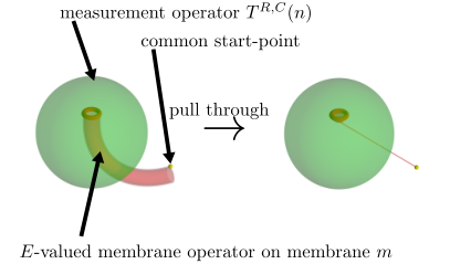
In order to find the charge of the loop-like excitation, we want to calculate
To do so, we must first evaluate
where and are stand-ins for any label that can appear for the individual operators in our measurement operators. Firstly, we note that commutes with , because both are diagonal in the configuration basis (the basis where each edge is labeled by an element of and each plaquette is labeled by an element of ). On the other hand does not commute with the magnetic membrane operator . We can see this by writing the surface element in terms of the constituent plaquettes, as
where is the label of plaquette and we have assumed each plaquette aligns with (otherwise we must replace the plaquette label with the inverse). We see that this depends on the group element associated to the path from the start-point of the membrane to the base-point of the plaquette. This path passes through the membrane and so is affected by the magnetic membrane operator. As we prove in Section S-IV.1.1 of the Supplemental Material (see Equation S72), such a path element satisfies the commutation relation
Defining
this leads to the surface label satisfying the commutation relation
so that
Then if we take the start-points of and to be the same (which has no effect on the result, because the start-point of the measurement operator can be changed without affecting the measurement operator), this becomes
where in the last line we used the fact that the contractible closed surface must have trivial label in the ground state, while the magnetic membrane operator applied on acts trivially on the ground state (again, because is closed and contractible). We can then use this result to evaluate the action of the measurement operator, to obtain
Then enforces that and so, just as with the calculation for the charge of the electric excitation, the groups involved in the projector simplify greatly. , the group of elements in which stabilise , becomes the whole group when . This also means that the sum over representatives becomes trivial, with being the only element. This gives us
| (52) |
Examining the term in brackets, , we see that treating as a coefficient for will result in this coefficient being decomposed into irreps of , describing the way in which the group acts on the coefficients by the action. Only the contribution from survives, due to orthogonality of characters, meaning that the measurement only gives a non-zero result if the coefficients contain the irrep . Therefore, the -valued loop can have a non-trivial spherical topological charge labeled by a representation of , depending on the choice of coefficients. If the coefficients are invariant under the action, so that for all and , then the term in brackets is zero unless is the trivial irrep, because must only contain the trivial irrep of . We note that this is the same condition for the start-point to be unexcited, as discussed in Section V.2, and so if the start-point is not excited then there is no point-like charge for the loop (this is to be expected, because if the start-point is not excited then it should not carry a charge to be balanced by the loop). However, if in general, then there will be some contribution from a non-trivial irrep. In particular, if for all (which is the condition for the start-point to definitely be excited, as proven in Section S-I C of the Supplemental Material for Ref. Huxford and Simon 2023b) then the contribution from the trivial irrep is proportional to
and so there is no contribution from the trivial charge measurement operator. This means that the point-like charge is definitely non-trivial if the start-point is excited.
IX.2 Topological charge within a torus
Now we consider measuring the topological charge using a toroidal surface. To do this, we first choose such a surface to measure on. Then we project onto the space where the surface has no excitations on it, so that we only measure the charge if no objects intersect the surface itself. This is to avoid the case where a loop excitation is only partially inside the measurement surface, because then we cannot unambiguously define the charge within the torus, as explained earlier in Section IX. A torus will allow us to measure both loop-like and point-like charge. One important thing to note is that the excitations that we measure need not lie inside the torus itself. Indeed we measure the loop-like charge of loop excitations that link with one of the cycles of the torus. For the meridian of the torus, those excitations will live inside the torus. However, the excitations that link with the longitude will be outside of the torus. This means that the torus surface can actually measure link-like excitations, made from loops outside the torus linking with those inside, rather than just loop-like excitations.
The topological charges measured by the torus are more numerous and mathematically complicated to derive than those measured by the sphere. We therefore first consider the case where is trivial (Case 1 from Table 1) as an introduction. As illustrated in Figure 42, we represent the torus surface as a rectangle with opposite sides identified. These sides are then one particular choice for the two independent cycles of the torus. We will choose to apply any membrane operators on this rectangle with the boundary at the cycles, before closing the rectangle by gluing the opposite edges. This leaves “seams” at the two cycles, which may have special properties because the action of the membrane operators on either side of the seam may not match. We can understand this by imagining taking a membrane operator applied on a rectangle and folding it up to glue the opposite edges together. There is no guarantee that a membrane operator acts the same on opposite sides of the rectangle, and this disparity may remain when we glue the sides together. We will see that this leads to additional joining conditions required to prevent additional excitations being present at these seams.
To find the measurement operators, we have to first project onto the case where the surface itself is not excited, then we see what degrees of freedom are left over. After projecting onto all of the plaquettes on the surface being flat, these two cycles of the torus are still left undetermined. We therefore apply two closed electric operators and , where and are the two cycles of the torus. We also apply a closed membrane operator on the torus, with the glued boundary of this torus being .
Requiring fake-flatness on the torus (this requirement follows from the plaquette terms) leads to the following constraint on the surface label of the torus and the labels and of the two cycles:
Together with the other conditions that we will discuss in this section, we prove this constraint in Section S-V.1 in the Supplemental Material. We can use the fact that is trivial to rewrite this constraint in a simpler way. When is trivial, conjugating an element by any element is trivial, because for all and . Then defining , we can write the above constraint in various ways. For example, we have
where in the fourth line we used one of the Peiffer conditions (Equation 1 in Section II) and in the last line we used the fact that is trivial. We can also write the condition as
| (53) |
Next we apply our magnetic membrane operator . Because we already projected to the subspace where the torus satisfies fake-flatness, some of the details of the operator are arbitrary; in particular the set of paths on the direct membrane, which affect the action on the edges, can be freely chosen, as long as these paths do not cross the seams of the membrane (we take this convention because two choices of path that differ by a non-contractible cycle may give different results and this gives us a consistent way of choosing the paths).
Finally, we apply blob ribbon operators around the cycles, so that our measurement operator so far is given by
In principle we could put closed blob ribbon operators anywhere on the membrane, rather than just on the cycles and . However, any blob ribbon operators with label in the kernel of can be freely deformed on the surface without affecting the action of the ribbon operators, because these operators are topological and there are no edge excitations on the surface (edge excitations in particular are relevant, because we deform blob ribbon operators by applying edge transforms, which are trivial when the edges are unexcited). This means that any such blob ribbon operator that does not wrap around a non-contractible cycle may be contracted into nothing, while an operator that does wrap around a non-contractible cycle on the torus may be deformed to wrap around the chosen cycles and (if the ribbon operator wraps both cycles, or wraps one multiple times, we split it into multiple ribbon operators on the cycles). This is not true for the other blob ribbon operators (those with label outside the kernel), because they are confined and so are not topological. Instead we find that this confinement leads to their position being fixed and their labels being restricted (as described in Section S-V.1 of the Supplemental Material), in order not to create any excitations. This is because the magnetic membrane operator may create plaquette excitations on the seams of the torus, but these excitations can be removed if the confined blob ribbon operators lie along the seam and have appropriate labels to cancel the effect of the magnetic membrane operator. We cannot place confined ribbon operators elsewhere (away from these seams) without producing new excitations. The appropriate labels for blob ribbon operators and , applied around the cycles and respectively, satisfy
| (54) | ||||
| (55) |
So far we have restricted the labels by requiring that our operator does not violate the plaquette conditions. However, we also need the combined operator to commute with the vertex and edge transforms on the surface so that the operator does not create vertex and edge excitations. This forces us to use linear combinations of operators with different labels. In particular, we show in Section S-V.1 of the Supplemental Material that we need an equal sum of the operators with sets of labels in certain equivalence classes. If two sets of labels must appear with equal coefficients in the linear combination, we denote this with an equivalence relation. We find the relations
| (56) | ||||
| (57) | ||||
| (58) | ||||
| (59) |
These conditions show a striking resemblance to the relations that appear in the calculation of the ground state degeneracy of the 3-torus in Ref. Bullivant et al. 2017 and indeed they map perfectly onto them in the trivial case. This indicates that the number of topological charges we can measure within a 2-torus is the same as the ground state degeneracy of the 3-torus in the -trivial case, as found more generally in Ref. Bullivant and Delcamp 2020.
We can repeat this calculation for the special case (Case 2 from Table 1) where we only enforce that is Abelian and centre(). Following the same argument as for the previous case (with full proofs given in Section S-V.2 in the Supplemental Material), we obtain the restrictions
| (60) | ||||
| (61) | ||||
| (62) | ||||
| (63) |
together with the equivalence relations
| (64) | ||||
| (65) | ||||
| (66) | ||||
| and | ||||
| (67) | ||||
These restrictions can again be mapped onto the ground state conditions given in Ref. Bullivant et al. 2017, as we demonstrate in Section S-V.2 in the Supplemental Material. This indicates that again there are the same number of ground states on the 3-torus as there are charges that can be measured by the 2-torus. We note that this relationship between the ground state degeneracy on the manifold and the charge sectors measured by the surface (with in this case being the 2-torus and being the 3-torus) is something we may expect for a TQFT Atiyah 1988.
We can use these conditions for the measurement operators to produce a set of projection operators that span the space of allowed measurement operators, just as we did for the spherical topological charge. Each such projector then corresponds to a particular value of topological charge. We find that these projectors are labeled by certain mathematical objects that were used by Bullivant et al. Bullivant and Delcamp 2020 when examining the ground states of the HLGT model. Specifically, each projector is labeled by a class of a particular space (to be described shortly) and an irrep of a particular group. To define these objects, we must follow some of the workings from Ref. Bullivant and Delcamp 2020. We note that some of our notation is slightly different from that paper, in order to match notation that we have previously used (and that was used in Ref. Bullivant et al. 2017). To understand , we must first define boundary -colourings. These are sets of three elements , where and . If this set satisfies , it is called a boundary -colouring Bullivant and Delcamp 2020. These sets are then divided into classes, by the equivalence relation Bullivant and Delcamp 2020
| (68) |
for each and . Then the label of the projector is one of these classes. The elements in are denoted by and is called the representative element of the class ( is an index that runs from 1 to the size of the class ) Bullivant and Delcamp 2020.
Expressions similar to the right-hand side of Equation 68 will appear frequently in this section, so we introduce some shorthand from Ref. Bullivant and Delcamp 2020, defining
| (69) |
where and are elements of and is an element of . We also introduce the notation from Ref. Bullivant and Delcamp 2020 that
| (70) |
where , and are elements of and and are elements of . Then using this notation, Equation 68 can be written as
| (71) |
In addition to the boundary -colourings, Bullivant et al. introduce sets of three elements , where and , with these sets of elements being called “bulk -colourings” Bullivant and Delcamp 2020. These colourings are also divided into classes, this time using an equivalence relation that depends on the boundary colouring. The equivalence relation is Bullivant and Delcamp 2020
for each . The corresponding set of equivalence classes is denoted by . Then for a class in the set , the elements in are denoted by
for The element is called the representative element for this class. A subset of these classes form a group called the stabiliser group of the class , Bullivant and Delcamp 2020:
where and the subscript in is to remind us that belongs to (and is interchangeable with the subscript ). The product for this group is defined so that the product of two classes and , , is the equivalence class in whose representative element is
The label of a projector to definite topological charge is an irrep of this stabilizer group.
Using the objects that we have discussed so far, we can finally define our projectors. First we define our product of individual membrane and ribbon operators:
| (72) |
Then we take appropriate linear combinations to construct the projector labeled by and :
In this expression, is the class in with representative element
where the and elements are defined as representatives which satisfy
and (that is the and move us around in the class to get from element to the representative element labeled by 1). In Section S-V.3 of the Supplemental Material we perform the lengthy algebraic task of proving that the operators labeled by the objects and form an orthogonal and complete set of projectors, indicating that the topological charges that we can measure with the torus are appropriately labeled by a class of boundary -colourings and an irrep of the corresponding stabiliser group.
X Conclusion
In this work, we have discussed in detail the features of the higher lattice gauge theory model in 3+1d. We started by constructing the ribbon and membrane operators which create the simple excitations of the model. We found that there were two categories of excitation, those best labeled by objects related to the group and those best labeled by objects related to the other group, . The former type of excitation, consisting of point-like electric excitations and loop-like magnetic flux tubes, are analogous to the excitations we expect from ordinary lattice gauge theory. The other type, consisting of point-like 2-gauge fluxes and loop-like 2-gauge charges, are related to properties of the surfaces of the lattice, instead of paths. We then considered the braiding properties of these excitations. When the map , defined as part of the crossed module, is trivial, these two types of excitations form separate sectors that do not have non-trivial braiding between them (only within each sector). However, when is non-trivial (although we had to restrict to the case where is Abelian and maps to the centre of ) some magnetic excitations acquire a 2-flux and can braid non-trivially with all other types of excitation. This is reflected in the fact the membrane operator that produces the magnetic excitation must be modified to depend on the surface elements of the lattice.
Another feature that we looked at was the condensation of certain excitations, and the accompanying confinement of others. We found that this was controlled by the map , with no condensation or confinement when maps only to the identity element (at least in the case where is Abelian). By altering while keeping the groups fixed, we introduce condensation for some of the loop-like (magnetic and -valued loop) excitations while causing some of the point-like (electric and blob) excitations to become confined. This can be thought of as a condensation-confinement transition, where the confined excitations are those that had non-trivial braiding with the condensed excitations. We also looked at the topological charge carried by the excitations, by constructing projectors to definite topological charge. The available charges depend on the surface of measurement, and we constructed the projectors for a spherical and toroidal surface. Similar to results found in Ref. Bullivant and Delcamp 2020, we found that the charges measured by the 2-torus surface matched the ground state degeneracy on the 3-torus. We saw that these 2-torus surfaces generally measured links, rather than simple loop-like excitations, suggesting that the number of inequivalent link-like excitations is equal to the ground state degeneracy.
In Ref. Huxford and Simon 2023a, we already mentioned several potential avenues of interest for further study based on this work. Rather than repeat ourselves here, we would like to discuss one of these directions further. In this paper, we gave braiding relations in terms of the simple excitations produced by the membrane and ribbon operators. However, it would be useful to obtain the braiding relations and other properties in terms of the topological charge. To do so, it would first be necessary to find the fusion rules for the various topological charges. Because the topological charge depends on the measurement surface, we would need additional machinery to describe how different charges can fuse in a simple way. Once this has been done, we can consider a braiding process where the individual excitations are projected onto states of definite charge, and the overall system is similarly projected to definite total charge, in order to find the braiding relations satisfied by the charges (analogous to the approach used for 2+1d theories). In addition to better understanding this particular model, creating this machinery would give us a structure with which to study different models for topological phases in 3+1d and understand what properties we expect. We note that, as mentioned in Ref. Huxford and Simon 2023a, from some preliminary calculations we can see that different torus charges can only fuse if they have the same value of a certain “threading flux”, meaning that the quantum numbers passing through the two loops must be the same (for example if they are linked to the same excitation). When this threading flux is non-trivial, we are considering the fusion of two loop-like excitations while both are linked to another excitation. This means that the braiding of these charges would correspond to so-called “necklace braiding” Bullivant et al. 2020 (or three-loop braiding Wang and Levin 2014), meaning the braiding of two loops while linked to another. For general models this braiding can give different results compared to the usual two-loop braiding Wang and Levin 2014; Jiang et al. 2014. Therefore, having a structure in which to consider this process for generic 3+1d topological models would be most useful.
Related to this idea, it would also be useful to understand better where the higher lattice gauge theory models fit into the wider landscape of 3+1d topological phases. It is conjectured that all 3+1d bosonic topological phases with bosonic point-like particles can be realised by Dijkgraaf-Witten theories Lan et al. 2018. This implies that the higher lattice gauge theories should also be equivalent to lattice gauge theory, albeit with some additional non-topological content in the form of the condensed and confined excitations. It would be interesting to explicitly demonstrate this equivalence (or else disprove it), whether through a direct mapping or by considering the topological charges and other data as we described above and showing that they match between the two models. We have made some progress in this direction, but leave the results for future study.
Acknowledgements.
The authors would once again like to thank João Faria Martins and Alex Bullivant for helpful discussions about the higher lattice gauge theory model. We are also grateful to Paul Fendley for advice on the preparation of this series of papers. We acknowledge support from EPSRC Grant EP/S020527/1. Statement of compliance with EPSRC policy framework on research data: This publication is theoretical work that does not require supporting research data.References
- Walker and Wang (2012) K. Walker and Z. Wang, (3+1)-TQFTs and topological insulators, Front. Phys. 7, 150 (2012).
- Wan et al. (2015) Y. Wan, J. C. Wang, and H. He, Twisted gauge theory model of topological phases in three dimensions, Phys. Rev. B 92, 045101 (2015).
- Williamson and Wang (2017) D. J. Williamson and Z. Wang, Hamiltonian models for topological phases of matter in three spatial dimensions, Ann. Phys. (N. Y.) 377, 311 (2017).
- Bullivant et al. (2017) A. Bullivant, M. Calcada, Z. Kadar, P. Martin, and J. F. Martins, Topological phases from higher gauge symmetry in 3+1D, Phys. Rev. B 95, 155118 (2017).
- Lan et al. (2018) T. Lan, L. Kong, and X.-G. Wen, Classification of (3+1)D bosonic topological orders: The case when pointlike excitations are all bosons, Phys. Rev. X 8, 021074 (2018).
- Lan and Wen (2019) T. Lan and X.-G. Wen, Classification of 3 + 1D bosonic topological orders (II): The case when some pointlike excitations are fermions, Phys. Rev. X 9, 021005 (2019).
- Doplicher et al. (1971) S. Doplicher, R. Haag, and J. E. Roberts, Local observables and particle statistics I, Commun. Math. Phys. 23, 199 (1971).
- Doplicher et al. (1974) S. Doplicher, R. Haag, and J. E. Roberts, Local observables and particle statistics II, Commun. Math. Phys. 35, 49 (1974).
- Pfeiffer (2003) H. Pfeiffer, Higher gauge theory and a non-Abelian generalization of 2-form electrodynamics, Annals of Physics 308, 447 (2003), arXiv:hep-th/0304074 .
- Baez and Huerta (2010) J. C. Baez and J. Huerta, An invitation to higher gauge theory, General Relativity and Gravitation 43, 2335 (2010).
- Gukov and Kapustin (2013) S. Gukov and A. Kapustin, Topological quantum field theory, nonlocal operators, and gapped phases of gauge theories, arXiv:1307.4793 (2013), 1307.4793 .
- Kapustin and Thorngren (2014) A. Kapustin and R. Thorngren, Topological field theory on a lattice, discrete theta-angles and confinement, Adv. Theor. Math. Phys. 18, 1233 (2014), 1308.2926 .
- Kapustin and Thorngren (2017) A. Kapustin and R. Thorngren, Higher symmetry and gapped phases of gauge theories, in Algebra, Geometry, and Physics in the 21st Century (Springer International Publishing, Cham, 2017) pp. 177–202, 1309.4721 .
- Huxford and Simon (2023a) J. Huxford and S. H. Simon, Excitations in the higher lattice gauge theory model for topological phases I: Overview, Phys. Rev. B 108, 245132 (2023a).
- Huxford and Simon (2023b) J. Huxford and S. H. Simon, Excitations in the higher lattice gauge theory model for topological phases II: the (2+1)-dimensional case, Physical Review B 108, 245133 (2023b).
- Kitaev (2003) A. Y. Kitaev, Fault-tolerant quantum computation by anyons, Ann. Phys. (N. Y.) 303, 2 (2003).
- Levin and Wen (2005) M. Levin and X.-G. Wen, String-net condensation: A physical mechanism for topological phases, Phys. Rev. B 71, 045110 (2005).
- Bombin and Martin-Delgado (2008) H. Bombin and M. A. Martin-Delgado, A family of non-Abelian Kitaev models on a lattice: Topological condensation and confinement, Phys. Rev. B 78, 115421 (2008).
- Bullivant and Delcamp (2020) A. Bullivant and C. Delcamp, Excitations in strict 2-group higher gauge models of topological phases, JHEP 01 (1).
- Baez (2002) J. C. Baez, Higher Yang–Mills theory, arXiv:hep-th/0206130v2 (2002).
- Bais (1980) F. A. Bais, Flux metamorphosis, Nucl. Phys. B 170, 32 (1980).
- Bucher et al. (1992) M. Bucher, K.-M. Lee, and J. Preskill, On detecting discrete Cheshire charge, Nucl. Phys. B 386, 27 (1992).
- Alford et al. (1992) M. G. Alford, K.-M. Lee, J. March-Russell, and J. Preskill, Quantum field theory of non-abelian strings and vortices, Nucl. Phys. B 384, 251 (1992).
- Wang and Levin (2014) C. Wang and M. Levin, Braiding statistics of loop excitations in three dimensions, Phys. Rev. Lett. 113, 080403 (2014).
- Jiang et al. (2014) S. Jiang, A. Mesaros, and Y. Ran, Generalized modular transformations in 3+1D topologically ordered phases and triple linking invariant of loop braiding, Phys. Rev. X 4, 031048 (2014).
- Bullivant et al. (2020) A. Bullivant, A. Kimball, P. Martin, and E. C. Rowell, Representations of the necklace braid group: Topological and combinatorial approaches, Commun. Math. Phys. 375, 1223 (2020).
- Bullivant et al. (2019) A. Bullivant, J. F. Martins, and P. Martin, Representations of the loop braid group and Aharonov-Bohm like effects in discrete (3+1)-dimensional higher gauge theory, Advances in Theoretical and Mathematical Physics 23, 1685 (2019).
- Komar and Landon-Cardinal (2017) A. Komar and O. Landon-Cardinal, Anyons are not energy eigenspaces of quantum double Hamiltonians, Phys. Rev. B 96, 195150 (2017).
- Atiyah (1988) M. F. Atiyah, Topological quantum field theory, Publ. Math. IHÉS 68, 175 (1988).
Supplemental Material
S-I The energy of ribbon and membrane operators
In this section, we will demonstrate the commutation relations of the ribbon and membrane operators with the energy terms in the 3+1d case, building on our results for the 2+1d case in Ref. Huxford and Simon 2023b (see Section S-I in the Supplemental Material of that paper).
S-I.1 Electric ribbon operators and -valued membrane operators
The commutation relations for the electric ribbon operators and -valued membrane operators with the energy terms are the same in 3+1d as in 2+1d (in our proofs in Ref. Huxford and Simon 2023b the dimension did not affect any of our workings), except that in 3+1d we also have blob energy terms. These blob terms are diagonal in the configuration basis (where all edges and plaquettes are labelled by group elements of and respectively), as are the electric ribbon and -valued membrane operators. Therefore, the electric ribbon operators and -valued membrane operators commute with the blob energy terms.
S-I.2 Blob ribbon operators
S-I.2.1 trivial case
Next we will demonstrate the commutation relations of the blob ribbon operators with the energy terms. We will first consider the case where is trivial (Case 1 from Table 1 in Section II of the main text).
As explained in Section III.4 of the main text, the blob ribbon operator acts along a string that passes from blob to blob, cutting through plaquettes along the way. For a blob ribbon operator labelled by the group element , each plaquette passed through (pierced) by the ribbon is acted upon by pre-multiplication by or post-multiplication by , depending on the orientation of the plaquette. If the circulation of the plaquette is obtained by applying the right hand rule to the direction of the ribbon then we post-multiply by , but if it is obtained by using the anti-right hand rule we instead pre-multiply by , as is illustrated by the example given in Figure 12 in Section III.4 of the main text. Because is Abelian when is trivial, whether we pre-multiply or post-multiply is irrelevant, it only matters whether or is used. Nonetheless, we use this language to match the other ribbon operators.
We want to consider the commutation relations of the blob ribbon operator with the energy terms. First we consider the blob energy terms. Consider a blob of arbitrary shape in the middle of the ribbon, i.e., not one of the blobs that the ribbon originates or terminates in. Every time the ribbon enters the blob it must also exit the blob, since the ribbon does not originate or terminate in this blob. We therefore want to consider the combined effect of the blob ribbon entering and exiting the blob on the blob energy term. The blob energy term measures the total surface element of the boundary of the blob and checks that this element is the identity. The surface element of the blob, in the trivial case, is a product of the individual plaquette elements on the surface, with an inverse if the orientation of the plaquette is opposite to the outwards normal of the blob (and no inverse if the orientation matches the outwards normal). That is, the 2-holonomy of a blob is
where Bd is the boundary surface of the blob and the in this surface are the constituent plaquettes that make up the boundary. is a variable that is 1 or , depending on the orientation of the plaquette.
The ribbon enters the blob by piercing a plaquette, which we will call plaquette 1, and exits by piercing another plaquette, plaquette 2, as shown in Figure S1. Suppose that these plaquettes have surface labels and respectively, before the action of the ribbon operator. If the orientation of plaquette 1 matches the outwards normal of the surface, then it does not match the orientation of the ribbon (whose direction is inwards to the surface here), as indicated in Figure S1. Therefore, in this case appears with no inverse in and the plaquette label becomes under the action of the blob ribbon operator. On the other hand, if the orientation of plaquette 1 does not match the outwards normal then its label appears as in but transforms to under the action of the blob ribbon operator. Therefore, the term in becomes . We see that regardless of the orientation of the plaquette, the term corresponding to that plaquette in gains a factor of . Similarly we can consider plaquette 2. For this plaquette, the outwards normal of the blob matches the orientation of the ribbon. Therefore, if the orientation of plaquette 2 matches the outwards normal, it appears as in and becomes under the action of the ribbon operator. On the other hand if the orientation of the plaquette is in the opposite direction, it appears as in the blob 2-holonomy and gains a factor of under the ribbon operator. Either way the term in gains a factor of . This means that under the action of the blob ribbon operator the blob 2-holonomy transforms as
where we used the Abelian nature of to cancel the factors of and . From this we see that the blob 2-holonomy is left invariant by the action of the blob ribbon operator. So far we have only considered the case where each blob is passed through precisely once by the ribbon. However, if a blob is pierced more than twice, we can still pair up the times where the ribbon enters and exits the blob as above, and so is still left invariant. We have therefore shown that the blob ribbon operator commutes with the blob energy terms, except perhaps for the blobs in which the ribbon originates and terminates.
Next we will consider these final blob terms, corresponding to the blobs in which the ribbon originates or terminates. Whereas blobs in the middle of the ribbon are both entered and exited by the ribbon, the blob at the start of the ribbon is only exited by the ribbon (unless the ribbon doubles back and passes through this blob again in which case the pass-through does not affect the energy term, as discussed above). Therefore, the blob 2-holonomy only gains the transformation from the plaquette through which the ribbon exits the blob, which was called plaquette 2 in the previous considerations. This means that the 2-holonomy gains a factor of from the action of the blob ribbon operator. On the other hand, the blob in which the ribbon terminates is only entered by the ribbon and not exited by it, so we only gain the transformation corresponding to plaquette 1. Therefore, the two-holonomy transforms as . This indicates that, when the blob ribbon operator acts on the ground state, it excites the two blobs at the origin and terminus of the ribbon, as long as is not the identity element of group (if is the identity element, then the blob ribbon operator is the identity operator).
Next we consider the vertex energy terms, which are made of a sum of vertex transforms . When is trivial does not affect the plaquette labels or interact with them in any way; instead the vertex transform only acts on the edge labels. Conversely the blob ribbon operator does not interact with the edge labels in any way. Therefore, the vertex transforms commute with the blob ribbon operators.
The next energy terms that we consider are the edge transforms. An edge transform will act on plaquettes neighbouring the edge by pre-multiplying the plaquette label by or post-multiplying by in the trivial case. This means that the order in which we apply an edge transform and a blob ribbon operator could at most determine in which order a plaquette label is multiplied (e.g., or ). However, because the group is Abelian the order of multiplication is irrelevant and so the edge transforms commute with the blob ribbon operators.
The final energy terms to consider are the plaquette fake-flatness terms. Recall that the plaquette energy term measures the plaquette holonomy and checks if this is the identity element in . The blob ribbon operator does not affect the path label but it can affect the plaquette label . If the ribbon pierces the plaquette then becomes or . Therefore, the action of the blob ribbon operator on the plaquette holonomy is
Therefore, if the plaquette holonomy is invariant under the action of the blob ribbon operator, and so the plaquette is not excited by the ribbon operator. On the other hand, if is outside the kernel of then the plaquette holonomy is changed by the action of the blob ribbon operator and so the plaquette is excited by the action of the ribbon operator. In this latter case, every plaquette pierced by the ribbon is excited and so the blob excitations are confined.
S-I.2.2 Fake-flat case
Next we consider the case where our crossed module is general, but we restrict our Hilbert space to only include fake-flat configurations (Case 3 in Table 1 of the main text). In this case the blob ribbon operators must be modified, as we described in Section V.3 of the main text. Firstly, to avoid violating fake-flatness, we must restrict the label of the ribbon operator to satisfy ; that is we only consider elements of in the kernel of . Secondly, it is necessary to introduce a configuration dependent part to the action of the ribbon operator, so that the action depends on the states of the edges along the ribbon. Instead of simply multiplying the plaquette labels on the path by or the inverse, we must first specify a vertex as the start-point of the ribbon operator, which we label by . Then the action on a plaquette , with base-point , is to pre-multiply the plaquette label by (or post-multiply by the inverse), where is a path from the start-point of the ribbon to the base-point of . An example of this action is shown in Figure 26 in Section V.3 of the main text. Explicitly, for a blob ribbon operator acting on a plaquette pierced by the ribbon, we have
| (S1) |
The precise path chosen between the start-point and the base-point of each plaquette does not matter when we are considering fake-flat configurations. This is because, given two paths with the same start and end-points that can be smoothly deformed into one-another, the paths enclose a fake-flat surface and therefore have the same label up to some element (although this is not the case if the paths together wrap some non-contractible cycle on the manifold). This means that given two paths and with the same start and end-points, which enclose a fake-flat surface, we have for some . If we chose as the path from the start-point of the ribbon operator to the base-point of the plaquette, then the plaquette label gains a factor of . On the other hand, if we chose , then the plaquette label gains a factor of
where the last equality follows from the second Peiffer condition (Equation 2 in the main text). However, when the label of the blob ribbon operator is in the kernel of it is also in the centre of (and therefore so is ). This also follows from the second Peiffer condition, which implies that, for any element , . Then the factor gained from choosing as the path from the start-point of the ribbon to the base-point of the plaquette is just
which is the same result we would obtain from choosing instead. Therefore, it does not matter which of and is chosen for , as long as the paths can be deformed into one-another. We note that this is only true because the element is taken to be in the kernel of , and this restriction will be relevant throughout this section.
Now we consider the commutation relations between the blob ribbon operator and the energy terms. We will first check the plaquette terms, which we enforce on the level of the Hilbert space rather than as an energetic constraint. Recall that the plaquette term for a plaquette is , where for plaquette label . Under the action of the blob ribbon operator, becomes or (depending on the orientation of the plaquette). If is in the kernel of , then so is for all and so . Therefore, the action of the blob ribbon operator preserves fake-flatness. On the other hand, if is not in the kernel of then is not invariant under the action of the blob ribbon operator, and so fake-flatness is violated. This is why we must restrict to be in the kernel of when we consider the fake-flat case.
Next we consider the other energy terms, which we do implement as ordinary energetic constraints. We first consider the vertex transforms. Unlike in the trivial case, the vertex transforms can interact with the blob ribbon operator in a number of ways. Firstly, the vertex transforms can affect the path labels which appear in the action of the blob ribbon operators. Secondly, the vertex transforms can directly affect the same plaquette labels on which the blob ribbon operator acts. Consider the action of the blob ribbon operator on the plaquette (or plaquettes) pierced by the ribbon that has its base-point at a particular vertex . The action of the blob ribbon operator on this plaquette (or plaquettes) is to multiply the plaquette label by or the inverse. The only vertex transforms which can affect the path label are the transforms at the start-point and at , because these are the two ends of the path. In addition, the only vertex transform that can affect the plaquette label directly is the transform at the base-point of the plaquette, . Therefore, when considering the action of the ribbon operator on the plaquette or plaquettes based at , the only vertex transforms which can fail to commute with this action are the vertex transforms at and at . We will first consider the transform at , , where we first assume that is not also the start-point of the ribbon (we treat the case where these vertices are the same afterwards). This vertex transform changes the path label to . In addition, the action of this transform on the plaquette is to take to . Therefore
This means that the vertex transform at commutes with the action of the blob ribbon operator.
Next we consider the vertex transform at the start-point of the ribbon, , assuming that the base-point of the plaquette we are considering, , is not the start-point. In this case, the vertex transform at the start-point does not directly change the plaquette label, but does change the path element . In particular, the transform takes to . Therefore
This suggests that , because this is true for the action on all plaquettes pierced by the ribbon and not based at the start-point. However, we have not yet considered plaquettes attached to the start-point itself and this relation must hold for all plaquettes for it to be an operator relation (it also must hold for any plaquettes not affected by the blob ribbon operator, but this holds trivially). That is, we now need to look at plaquettes for which the base-point is also the start-point of the ribbon . For these plaquettes, the path is the trivial path (or at least is a closed path, with label in the image of from fake-flatness) and so is not changed by the vertex transform. However, the vertex transform directly affects the plaquettes that have as their base-point. Therefore
We see that the action of the two operators on such plaquettes obeys the same commutation relation as the action on plaquettes not based at the start-point. Therefore, the relation holds for all plaquettes, and so the operators satisfy the commutation relation
| (S2) |
This means that the start-point vertex may be excited by the blob ribbon operator, depending on which linear combination of the blob ribbon operators is taken. Consider a linear combination of the operators . Then
If for all in the kernel of , then we see that the vertex transform commutes with the ribbon operator. Because the vertex energy term is , this means that if for all and , then the ribbon operator commutes with the vertex transform at the start-point and so does not excite the vertex. On the other hand, consider applying the ribbon operator on the ground state, or some other state for which the start-point is not excited. Then consider
If this is zero it means that the ribbon operator excites the start-point (recall that is a projector with the zero eigenvalues corresponding to excited states). If the start-point is not excited in then . Therefore
where in the last line we used that . Then if , we have that and so the vertex is excited.
Having examined the commutation relation between the blob ribbon operator and the vertex transforms, we next consider the edge transforms. The edge transform affects both path elements and surface elements, so we must check that neither of these effects fail to commute with the action of the blob ribbon operator. An edge transform can affect the path label , by changing an edge label by . This means that if we act first with the edge transform and then the blob ribbon operator, instead of in the action of the ribbon operator we will have , where and represent the parts of the path element on either side of the edge. However, we will see that the edge transform does not affect the label . We have that from the Peiffer conditions (see Equation 2 in the main text). In addition the label of the blob ribbon operator is in the centre of , which also means that is in the centre as well (as discussed in Section V.3 of the main text). This means that we can cancel the factors of and and so the expression is unchanged by the edge transform. Therefore, the action of the edge transforms on the edge labels commutes with the blob ribbon operators. We still need to consider the action of the edge transforms on the surface labels however, because both the blob ribbon operators and edge transforms act on the surface labels. The edge transform multiplies the neighbouring surface labels by some , where is a path element as described in Section II of the main text. Similarly, the blob ribbon operator multiplies surface labels by some , where is again a path label as described at the beginning of this section. However, because is in the centre of , each is also in the centre of . This means that the order in which we apply the multiplication from the blob ribbon operator and edge transform is irrelevant, because the factors commute. Therefore, the edge transforms (and so the edge energy terms, which are linear combinations of the edge transforms) commute with the blob ribbon operator.
The final energy terms to consider are the blob energy terms. Just as in the trivial case, we will consider the effect of the blob ribbon entering a blob on the blob 2-holonomy and show that this effect cancels with the effect of the ribbon leaving the blob. Therefore, only the blobs in which the ribbon originates or terminates (the blobs which have an imbalance between the ribbon entering and leaving the blob, in the simplest case only entering or leaving the blob) will be excited by the action of the blob ribbon operator. To see this, consider the blob 2-holonomy of a blob . This is given by
where is the base-point for the blob (which one is chosen does not matter). Note that, while the product over plaquettes should be taken in a specific order and the paths appearing must also be chosen appropriately (the order and precise paths must follow the rules for combining surfaces that we summarized in Section II), we will not need to specify these details for this argument. The are or depending on the orientation of the plaquette , as discussed in the trivial case in Section S-I.2.1. When the blob ribbon operator enters the blob, it multiplies one plaquette by . By the same argument as for the trivial case in Section S-I.2.1, while the plaquette can be multiplied by or the inverse, the term is always multiplied by (because the orientation of the plaquette relative to the blob normal is opposite to the orientation with respect to the blob ribbon). Therefore, the term for the plaquette pierced by the blob ribbon when it enters the blob becomes
Because is in the centre of (due to being in the kernel of ), the precise path appearing in an expression does not matter (or rather, any two paths and that can be deformed into one-another over a fake-flat surface will give the same result, as described in Section V.3 of the main text). Therefore, we can write without needing to worry about the precise choice of path in each case. In addition, because is in the centre of , we can extract the factor to the front of the product in . Putting these ideas together, the transformation of from the ribbon entering the blob is
| (S3) |
Next we consider the effect of the ribbon leaving the blob on the blob 2-holonomy. Just as the ribbon entering the blob has the effect of multiplying one term by , the ribbon exiting the blob multiplies one by (because the orientation of the blob’s normal matches the orientation of the ribbon in the place that the ribbon exits the blob). Just as before, we can extract this factor to the left and write to find that the effect of the ribbon leaving the blob is
| (S4) |
We see that the effects of the blob ribbon entering and exiting a blob on the blob’s 2-holonomy cancel, so the blob ribbon operator does not excite the blob energy terms for blobs in the middle of the ribbon. On the other hand, for the blobs at the origin and terminus of the ribbon there is no such cancellation, so the ribbon operator excites the blob energy terms.
S-I.2.3 The case where centre() and is Abelian
The final case that we consider is where the group is Abelian and the map from to maps on to the centre of (Case 2 in Table 1 of the main text). In this case, we can define the blob ribbon operators with any label from , rather than just from the kernel of . The blob ribbon operators are defined in the same way as in the fake-flat case considered in the previous section: when acting on a plaquette based at , the blob ribbon operator acts on the plaquette label as
| (S5) |
We want to consider the commutation relations of the ribbon operator with the energy terms. The commutation relations mostly follow from our arguments in the previous section. First we consider the plaquette term. If the label of the blob ribbon operator is not in the kernel of , then the blob ribbon operator will change the of all plaquettes through which it passes and so will excite the plaquettes, as described in the previous section. Unlike in the previous section, we do not need to throw out the ribbon operators which violate fake-flatness, because we allow fake-flatness violations in our Hilbert space. Instead, the ribbon operators which excite the plaquette terms create confined blob excitations, because there is an energy cost associated to the length of the ribbon used to create them.
Note that, while some ribbon operators excite the plaquette terms, they only break fake-flatness by an element for some (because they change the plaquette surface label and not the edge labels around the plaquette). This is significant, because it means that two paths that enclose a surface where fake-flatness is violated in such a way only differ in label by some element on top of the factor expected from deformation over the surface. In the case we are considering, an extra element of in a path label does not affect certain expressions. In particular a factor of in a path element does not affect (from , using Abelian) or (from , using the fact that maps in to the centre of ). Because of this, such violations of fake-flatness do not affect the composition of surfaces (which relies on fake-flatness in order to be invariant under changing the branching structure) and so do not obstruct the sensible definition of blob energy terms (which rely on composing plaquettes into the surface of the blob) in the region of the ribbon.
For the other energy terms, the commutation relations with the blob ribbon operator are exactly as we considered in Section S-I.2.2. We can follow that argument precisely, except without the requirement that the label of the blob ribbon operator be in the kernel of , because we only used the fact that the label was in the centre of in the previous argument (and when is Abelian this is true for all ). That is, the blob ribbon operator commutes with all edge transforms, all vertex transforms except potentially the one at the start-point of the ribbon and each blob energy term except the ones for the blobs in which the ribbon originates or terminates. The commutation relation of a blob ribbon operator with a vertex transform as the start-point of is the same as Equation S2:
| (S6) |
Similarly the transformation of the 2-holonomy of a blob entered by the ribbon is
| (S7) |
which is the same as Equation S3, while the transformation of a blob exited by the ribbon is
| (S8) |
which is the same as Equation S4. These two transformations cancel for a blob which is both entered and exited by the ribbon (i.e., that is passed through by the ribbon).
We have therefore shown that the blob ribbon operator excites the blobs at the origin and terminus of the ribbon. In addition the blob ribbon operator excites the plaquettes pierced by the ribbon if is outside the kernel of . Finally the start-point of the ribbon may be excited, depending on which linear combination is considered. Note, however, that we have assumed that the state on which we act with the blob ribbon operator satisfies fake-flatness in the region on which we apply the ribbon (for example when considering the blob conditions along the ribbon). If it does not, the ribbon may cause some additional excitations.
S-I.2.4 Fusion of blob ribbon operators
We can combine two blob ribbon operators that are applied on the same ribbon (which means they must have the same start-point) into a single ribbon operator. Consider the action of two blob ribbon operators, and , on a plaquette pierced by the ribbon . We have
This holds for all plaquettes , so it gives us the operator relation
| (S9) |
S-I.2.5 Reversing the orientation of the dual path
When defining the blob ribbon operator in the preceding sections, we used the concept of a dual path. The plaquettes in the lattice which are pierced by the dual path are acted on by the blob ribbon operator. The relative orientation of the dual path and the plaquette determines the action of the blob ribbon operator on the plaquette. It is therefore useful to see what happens when we invert the orientation of this dual path. Given a plaquette pierced by a blob ribbon operator the action of the blob ribbon operator on the plaquette is
Now consider what happens when we reverse the orientation of the dual path, to produce a new ribbon . A blob ribbon operator applied on this ribbon acts on the plaquette as
If we write this in terms of the orientation of the original ribbon, , this becomes
Then we can use the fact that we only consider blob ribbon operators whose labels lie in the centre of (either because is Abelian, or because we restrict to the fake-flat case when is non-Abelian), to rewrite this as
Comparing this to the action of , we see that
That is, the new ribbon operator acts in the same way on the plaquette as a blob ribbon operator on the original ribbon but with inverted label. This holds for all plaquettes , so we can write this as an operator relation:
| (S10) |
If we invert this relation, we obtain
| (S11) |
That is, the ribbon operator is unchanged if we simultaneously invert its label and the orientation of its dual path. In other words, we can invert the orientation of the dual path of a blob ribbon operator by inverting the label of the blob ribbon operator, without affecting the action of the ribbon operator. Note that we have not changed the direct path of the ribbon operator, so now the first plaquette affected by the reversed ribbon operator is at the end of the direct path.
S-I.2.6 Moving the start-point of a blob ribbon operator
When is non-trivial, the action of the blob ribbon operator on a plaquette depends on a path from a special vertex, called the start-point of the ribbon operator, to the base-point of the plaquette being acted on. It is worth considering what happens to the ribbon operator when we change this start-point. Consider a blob ribbon operator acting on a ribbon , whose start-point is . We then move the start-point to a new position, , while keeping the dual path of the ribbon fixed (i.e, the ribbon operator still acts on the same plaquettes), as shown in Figure S2. Let the initial blob ribbon operator be , while the final ribbon operator is . The action of the original ribbon operator on a plaquette pierced by the ribbon is
where is the base-point of the plaquette .
Similarly the action of the new ribbon operator on the same plaquette is
If we moved the start-point along the path when we changed the start-point, then we can write the path as . Therefore, denoting the label of path by , we have
Substituting this into the action of , we see that
We see that the ribbon operator acts on plaquette in the same way as . This holds for all plaquettes (recall that and have the same dual path and so the corresponding ribbon operators act on all the same plaquettes). Therefore, we can write that
| (S12) |
We have seen that moving the start-point of a blob ribbon operator, while keeping the label constant, changes how the operator acts. We can also change the start-point and simultaneously change the label of the operator, in order to keep the action of the operator fixed. That is, we can describe the same blob ribbon operator in different ways by choosing different start-points and taking appropriate labels for each (this is analogous to a choice of basis). For an initial blob ribbon operator , we wish to find the label of blob ribbon operator such that . To do this, we just need to invert Equation S12. We therefore see that
| (S13) |
Note that the label of the blob ribbon operator includes the path label , so the ribbon operator label is actually an operator. This reflects the idea that the 2-flux produced by the blob ribbon operator is well-defined with respect a particular start-point ( in this case), but not with respect other start-points (a fact that is important when we consider braiding).
When considering Equation S12, we can see a great similarity with Equation S6, which describes the commutation relation between the blob ribbon operator and the vertex transform at the start-point. Indeed the transformation of the blob ribbon operator when we move the start-point along a path of label is the same as the transformation when we apply the vertex transform . This reflects the idea that we discussed in Ref. Huxford and Simon 2023a, that applying the vertex transform on a vertex is equivalent to parallel transporting that vertex along a path of label . For this reason, a blob ribbon operator that commutes with the vertex energy term at the start-point is also unaffected by moving its start-point. Mathematically, this occurs because a blob ribbon operator that commutes with the start-point vertex transform has the form , and so any additional action on the label can be absorbed into the sum over .
S-I.2.7 Concatenation of blob ribbon operators
In the previous section, we described the procedure by which we move the start-point of a blob ribbon operator. In this section, we will describe one reason we may wish to do this: the joining of two ribbons together into a longer one. Consider two blob ribbon operators and , whose dual paths connect together so that they form an unbroken path through a series of plaquettes, as shown in Figure S3. We may wonder whether these two ribbon operators can be written as a single ribbon operator acting on the combined path. This may be true, but the two blob ribbon operators must satisfy certain conditions for this to be the case.
Suppose that the product of the two blob ribbon operators can be written as a single blob ribbon operator , whose dual path is the concatenation of the dual paths of the other two ribbon operators. Then the action of must agree with the action of on the plaquettes pierced by and with the action of on the plaquettes pierced by . The action of on a plaquette pierced by is
If the plaquette is pierced by , then the action of on is
where we used the fact that and have the same orientation to write the two cases in terms of the orientation of instead of . We see that these actions are the same if the labels satisfy
If we choose the start-point of to be the same as the start-point of , then this condition becomes , so the total ribbon operator must be . We now wish to see when the action of the other ribbon operator, , agrees with the action of on the other section of path. The action of on a plaquette pierced by is
This agrees with the action of when the labels satisfy
where . If the paths and are the same, or can be deformed into one-another over a fake-flat surface, then the condition becomes . A necessary condition for this is that the start-points of the two ribbons are the same (if the region is not fake-flat, or there are non-contractible cycles, then we must take further care that the direct paths of the two ribbons are compatible). On the other hand, if the start-points are different, then we can move the start-point of to match the start-point of , and then the labels must match. To see this, we can write
We then note that is the label we must give the blob ribbon operator when we change its start-point from to , if we wish to keep the action of the blob ribbon operator constant (see Equation S13). Then the condition
can be written as
which implies that . That is, the label of the two blob ribbon operators that we wish to combine must match, once we move the start-points of the ribbon operators to the same position.
S-I.3 Magnetic membrane operators in the trivial case
In this section we derive the commutation relations of the magnetic membrane operator with the energy terms, in the case where is trivial. Recall from Section III.2 of the main text that the magnetic membrane is characterised by two membranes: the dual membrane and the direct membrane. These are illustrated in Figure 7 in Section III.2. The dual membrane intersects a set of edges and it is these edges that are acted on by the membrane operator. The direct membrane contains a set of vertices at one end of each of these edges. The action of the magnetic membrane operator on each edge depends on the path element for the path from a privileged start-point to the vertex in the direct membrane attached to the edge in question. The action of a magnetic membrane operator on an edge element of an edge cut by the dual membrane is to either pre-multiply the edge element by or post-multiply it by the inverse, where is the relevant path element from the start-point of the membrane, , to the vertex that lies on the direct membrane and is attached to edge . If the edge points away from the vertex (i.e., away from the direct membrane) then it is pre-multiplied by , and if it instead points towards the vertex (towards the direct membrane) the edge element is instead post-multiplied by . We can summarize this action on an edge cut by the dual membrane as
| (S14) |
Now we want to consider the commutation relations of this operator with the energy terms. We start by considering the vertex transforms. Just as in the 2+1d case considered in Ref. Huxford and Simon 2023b (see Section S-I B in the Supplemental Material for that paper), the vertex transforms may interact with the magnetic membrane operator in two ways. The first way is by directly affecting the edges whose labels are changed by the magnetic membrane operator: the edges that are cut by the dual membrane. An edge label is affected by vertex transforms at the two ends of the edge, so these transforms may fail to commute with the magnetic membrane operator. The second way in which a vertex transform may fail to commute with the membrane operator is if the vertex transform affects the path labels that appear in the action of the magnetic membrane operator on an edge (see Equation S14). As we proved in Section S-I A of the Supplemental Material for Ref. Huxford and Simon 2023b, a vertex transform affects the labels of paths that start or end at that vertex, so we must consider the vertex transforms at the start-point of the membrane, , and the vertex for each edge cut by the dual membrane. We note that because the vertex is attached to the edge , a vertex transform at also directly affects the label of the edge .
Considering these two ways in which the vertex transforms can interact with the magnetic membrane operator, we see that there are three classes of vertex to consider. The first is the set of vertices which are attached to edges that are cut by the dual membrane, but which do not lie on the direct membrane. The transforms on these vertices directly affect the labels of the edges cut by the dual membrane, but do not affect the path labels which appear in the action of the membrane operator. The second class of vertices is the set of vertices which both lie on the direct membrane and are attached to edges cut by the dual membrane, except the start-point. The vertex transforms on these vertices directly affect the edges cut by the dual membrane and also affect the path labels which appear in the action of the membrane operator. The final type of vertex is the start-point vertex itself, which can also directly affect some edges, and also acts on the path labels for every edge cut by the membrane (because all of the paths start at the start-point).
We start by considering the first class of vertices, those which do not lie on the direct membrane but are attached to edges cut by the dual membrane. Recall that each edge is attached to two vertices (the source and target of the edge), and for the edges intersected by the dual membrane one of these vertices lies on the direct membrane and one of them lies away from it (unless the membrane folds back on itself). However, the vertex transforms on the end of the edge not on the direct membrane will commute with the membrane operator. To see this, first note that the action of a vertex transform on an edge attached to the vertex is
That is, the vertex transform either left-multiplies the edge label by or right-multiplies it by , depending on the orientation of the edge. The membrane operator also left-multiplies the label of an edge cut by the membrane by some element or right-multiplies it by the inverse, depending on the orientation of the edge if the edge points towards the direct membrane. For the vertex attached to the edge but away from the direct membrane, if the edge points away from the direct membrane it points towards the vertex (and vice-versa). This means that, when the membrane operator right-multiplies the edge label by some element (because the edge points away from the membrane), the vertex transform left-multiplies it by another element (because the edge points towards the vertex), and vice-versa. Therefore, applying the magnetic membrane operator and then the vertex transform has the following action on the edge :
Because one of the operators right-multiplies the edge label while the other left-multiplies it (and the group elements involved are independent), the contributions from the two operators commute. This means that the vertex transforms away from the direct membrane commute with the magnetic membrane operator.
Next we consider vertex transforms on the vertices in the direct membrane, which can act on the same edges as the magnetic membrane operator and affect the path elements that appear in the action of the magnetic membrane operator. Just as we did for the ribbon in the 2+1d case in Ref. Huxford and Simon 2023b (see Section S-I B of the Supplemental Material), we group the edges that are cut by the dual membrane according to which vertex in the direct membrane they are attached to. We do this because edges attached to the same vertex are acted on by the membrane operator in a similar way. The action on these edges depends on a path element , so we want to consider which vertex transforms can change this path element. Recall that the only vertex transforms that affect a path label are the transforms at the start and end of the path. The start of this path is the start-point of the membrane, which is the same point for each path that we will consider (the start-point is a property of the membrane, independent of which vertex we consider). On the other hand, the end of this path is , the vertex for which we are considering the attached edges, as shown in Figure S4. We therefore only need to consider the vertex transforms on these two vertices, starting with the ones at .
We will see that the vertex transforms at commute with the magnetic membrane operator, in exactly the same way that the analogous vertex transform commutes with the magnetic ribbon operator in the 2+1d case. The fact that we have three spatial dimensions rather than two makes no difference, because we do not need to worry about the geometry when considering the edges attached to a particular vertex. Nonetheless, we sketch the proof again here. We consider the situation where we apply the magnetic membrane operator followed by vertex transform on the vertex and compare this to the case where we apply the operators in the opposite order.
We call the edges which are affected by both the magnetic membrane operator and the vertex transform (i.e., the edges attached to the vertex which are also cut by the dual membrane, which are the bright red edges in Figure S4) the shared edges. The other edges attached to the vertex are only affected by the vertex transform, so the action on these edges is the same regardless of the order in which we apply the operators. For a shared edge , with label , acting first with the magnetic membrane operator and then with the vertex transform gives
On the other hand, if we act with the operators in the opposite order takes the path element to before the membrane operator acts (because the vertex is at the end of the path), so that we have
The combined action of the two operators is the same for either order, so the action of this vertex transform commutes with the action of the magnetic membrane operator on the edges attached to these vertices. Since the vertex transform does not affect any other edges that are cut by the membrane operator, or affect any path labels which appear in the magnetic membrane operator (other than the ones terminating at ), this means that the vertex transform commutes with the magnetic membrane operator.
The final vertex transform to consider is the one at the privileged start-point of the membrane, . Just like in the 2+1d case, the vertex transform takes all of the path labels that appear in the action of the membrane operator to (as shown in Section S-I A of the Supplemental Material for Ref. Huxford and Simon 2023b) and so takes the factor to . This holds for all vertices except for the start-point itself. This means that when acting on an edge attached to a vertex that is not the start-point, we have
which suggests that . However, for this commutation relation to hold it needs to be true for the action on every edge, including the edges attached to the start-point itself. For such an edge, initially labelled by , we have
Therefore, the relation holds for every edge, meaning that we have the operator relation
| (S15) |
Because the vertex transform at the start-point does not commute with the membrane operator, when we take linear combinations of the membrane operators with label in the conjugacy class of , the start-point may be excited, just as in the 2+1d case examined in Ref. Huxford and Simon 2023b (specifically, it is not excited if the coefficients of the linear combination are a function of conjugacy class, and is excited if the coefficients within the conjugacy class sum to zero).
Next we consider the edge transforms, which can seemingly interact with the magnetic membrane operator in two ways. Firstly, they change the value of a path element appearing in the membrane operator if the edge on which we apply the transform lies on that path. However, just as we saw in the 2+1d case in Ref. Huxford and Simon 2023b (see Section S-I B of the Supplemental Material), while the edge transforms can affect the value of a path element, they always leave invariant when is trivial. This is because gains a factor of for some from the edge transform, and gains a factor of . However, when is trivial factors in are in the centre of , so the two factors of and can be commuted together and cancelled. The second way in which we may think that the edge transforms and magnetic membrane operator could interfere is by the transforms acting on the same edges that have their labels changed by the magnetic membrane operators (those edges cut by the dual membrane). However, the edge transforms on the edges cut by the dual membrane only change these edge labels by an element , which is again in the centre of and so commutes with the factors added by the magnetic membrane operator. Therefore, all edge transforms commute with the magnetic membrane operators.
Now consider the plaquette energy terms. The plaquettes that may be affected are those where some of the edges on the plaquette are cut by the dual membrane of the membrane operator. We divide such plaquettes into two classes. Firstly, we have the plaquettes which are pierced by the boundary of the dual membrane (the plaquettes which we claimed were excited by the membrane operator in Section III.2 of the main text). For these plaquettes, only one edge is cut by the dual membrane (assuming the dual membrane does not fold in on itself and cut the same plaquettes or edges multiple times, as in the case shown in Figure S6). We refer to such plaquettes as boundary plaquettes. Secondly, we have the internal plaquettes, where the dual membrane cuts through two edges. We will see that the effect of the membrane operator on these two edges cancels in the expression for the plaquette holonomy and thus leaves the plaquette energy term unaffected. Consider such an internal plaquette cut by the membrane, with two edges affected by the membrane operator, as shown in Figure S5. We are free to choose the base-point and orientation of the plaquette without affecting the energy term (as we showed in the Appendix of Ref. Huxford and Simon 2023a), so the plaquette in the figure is generic. The plaquette holonomy is then given by
Under the action of the magnetic membrane operator , this becomes
Note that the path is a closed loop. As long as this closed loop forms the boundary of a fake-flat surface (before we apply the transform), we know that for some from the fake-flatness condition. This means that . Making this substitution in the expression for the plaquette holonomy above gives
Then using the fact that elements of are in the centre of , we can cancel the factors of and its inverse, to obtain
from which we see that the plaquette holonomy is simply conjugated by an element by the action of the membrane operator. Conjugation preserves the identity element, so the magnetic membrane operator does not excite this internal plaquette. This means that the magnetic membrane operator can only excite the boundary plaquettes.
For these boundary plaquettes, only one edge on the plaquette is affected by the membrane operator, and so the plaquette holonomy only gains one factor of or the inverse, meaning that there is no cancellation and the plaquette is excited unless . In particular, the plaquette holonomy becomes
| (S16) |
or
depending on which edge on the plaquette is cut by the membrane operator and the orientation of the plaquette.
We should note that our argument that the internal plaquettes are not excited by the membrane operator relies on the path enclosing a fake-flat surface. If this is not the case (for example, if these paths enclose an excited plaquette, created by another magnetic excitation) then the plaquette may be excited by the membrane operator. We already discussed some such cases in Section IV.2.3 of the main text, where we consider the case where two magnetic flux tubes link together, and we will examine this linking phenomenon in more detail in Section S-IV.1.4. In using Figure S5, we also implicitly made some assumptions about the shape of the membrane, in particular that it does not fold over and cut the same plaquette more than once. An example of a case where the membrane does cut the same plaquette more than once is shown in Figure S6. However, we do not need to make such an assumption. These cases can be dealt with by separately considering each instance where the membrane cuts through the plaquette and then treating each instance in the way we have previously in this section (by pairing the edges cut each time the membrane passes through the plaquette and noting that the effect of such a pair on the plaquette holonomy cancels).
The final energy terms to consider are the blob energy terms. When is trivial the blob energy term only acts on the plaquette labels, which are not affected by the magnetic membrane operator. This means that the blob energy term commutes with the magnetic membrane operator. Combining this with our previous results for the commutation relations between the magnetic membrane operator and the energy terms, we see that the membrane operator only excites the boundary plaquettes around the membrane (the plaquettes pierced by the boundary of the dual membrane) and potentially the start-point vertex (depending on which linear combination of magnetic membrane operators we take).
S-I.3.1 Changing the start-point
We have seen that the action of the magnetic membrane operator depends on our choice for a privileged vertex, which we called the start-point. The action of the magnetic membrane operator on an edge cut by the dual membrane is given by
which depends on the start-point through the path element . It is therefore interesting to consider what happens when we change this start-point. Imagine moving the start-point from to a new position, , along a path . We denote the membrane with this new start-point by . The action of the membrane operator on an edge cut by the dual membrane is then
When we move the start-point along , we drag all of the paths with the start-point, so that the new paths are . This means that the path element can be written as . Substituting this into the action of , we see that
where in the last line we wrote the action in terms of a membrane operator on the original membrane (with original start-point ). This holds for the action on all edges , so we can write this in terms of the operators as
| (S17) |
We see that moving the start-point of the membrane operator is equivalent to changing the label of the operator, by conjugating the label by the path along which we move the start-point. Note the similarity with the transformation of the magnetic membrane operator under commutation with the vertex transform at the start-point, as described by Equation S15. Commutation with the vertex transform also conjugates the label of the magnetic membrane operator, in this case by the label of the vertex transform. As we discussed in Ref. Huxford and Simon 2023a, applying a vertex transform on a vertex is similar to parallel transporting that vertex along an edge labelled by , and so it is not surprising that moving the start-point of the membrane operator should have a similar effect to applying a vertex transform at the start-point. This also means that a magnetic membrane operator that is invariant under the vertex transforms (i.e., a magnetic membrane operator that produces no excitation at the start-point) is also invariant under a process by which we move the start-point.
So far, we have considered moving the start-point of the membrane operator while keeping its label fixed, and have seen how this changes the action of the membrane operator. Just as we did with the blob ribbon operators in Section S-I.2.6, it is also useful to consider how we can change the label as we move the start-point in order to keep the action of the membrane operator fixed. That is we want to find the label such that . To find , we use Equation S17 and invert the transformation implied by that equation, to obtain
| (S18) |
S-I.4 Magnetic membrane operators in the case where centre() and is Abelian
We now consider the magnetic excitations in the case where is Abelian and is in the centre of (Case 2 from Table 1 of the main text). Restricting the crossed module in this way allows us to simplify many expressions that we use throughout this section. Firstly, recall that the crossed module satisfies the Peiffer condition for all elements . When the group is Abelian, this relation simplifies to . This has important consequences when we consider expressions such as , where is a path element. Two paths, and , which can be deformed into one-another over a fake-flat surface differ in label only by some element . This is because the closed path is a closed path enclosing a fake-flat surface and so must have a label in . This means that, for any element , the two path elements satisfy . Therefore, whenever we have a path element acting on a surface label in this way, we can freely deform the path that we are considering without changing the result, as long as we only deform the path across a fake-flat surface. One consequence of this and the Abelian nature of is that the calculation of the 2-holonomy of a blob becomes simple. For a blob , based at a vertex , the blob 2-holonomy is given by
| (S19) |
where is if the plaquette’s orientation (determined using the right-hand rule) points outwards from the blob and is if the orientation points inwards. In the case of the most general crossed module, the order of the product and the choice of paths for each are important (and should follow the rules for combining surfaces that we summarized in Section II). However, because is Abelian, the order of multiplication is irrelevant. In addition, because we can deform the paths without affecting , the precise choice of path does not matter provided that the region around the blob satisfies fake-flatness.
Another useful result arises from the other Peiffer condition for all and . Because we have restricted our crossed module so that is within the centre of , this Peiffer condition implies that . This means that expressions of the form are in the kernel of for any and . Another consequence of this restriction on is that, given a path and an expression of the form , we can freely deform the path over a fake-flat region without changing the expression. This is because deforming the path over such a region just changes the path label by an element . Then, because is in the centre of , the contributions of this factor to cancels with its contribution to :
S-I.4.1 Definition of the magnetic membrane operator
Having considered some of the consequences of restricting the crossed module in this way, we can discuss the magnetic membrane operator in this case. In order to define the magnetic membrane operator, we define two operators. Firstly we introduce the operator . This operator acts on edge labels in the same way as the magnetic membrane operator from the trivial case (see Equation S14 in Section S-I.3), but also affects the surface labels of plaquettes that are cut by the dual membrane. For an unwhiskered plaquette that is cut by the dual membrane, the base-point of the plaquette either lies on the direct membrane or away from it, in which case it is separated from the direct membrane by the dual membrane. If a plaquette cut by the dual membrane of the operator has its base-point on the direct membrane of the membrane operator then the label of the plaquette goes from to , where is a path from the start-point of the membrane operator to the base-point of the plaquette. If the base-point of the plaquette is away from the direct membrane, so that the dual membrane lies between the base-point and the direct membrane, then it is not affected. That is, the action of on an unwhiskered plaquette cut by the dual membrane of is
| (S20) |
where is the base-point of plaquette . This action is reminiscent of the vertex transforms, which only affect the surface labels of plaquettes which are based at the vertex on which we apply the transform. Note that we specified an unwhiskered plaquette, meaning plaquettes that do not have sections of boundary that enclose no surface and can be removed by moving the start-point. If we consider a whiskered plaquette, then the base-point of the plaquette could lie anywhere, and in particular the base-point could be whiskered through the direct membrane (on the other side to the dual membrane), and so neither lie on the direct membrane nor are separated from the direct membrane by the dual membrane. We will not consider such plaquettes directly, but we can define the action of the magnetic membrane operator on such plaquettes indirectly by demanding that the action of the membrane operator be consistent with the “re-branching” procedure from Ref. Huxford and Simon 2023a where we move the base-point of a plaquette along path and simultaneously change its label from to (we will show in Section S-I.4.2 that the action of the magnetic membrane operator on unwhiskered plaquettes defined by Equation S20 is consistent with this procedure, but will not consider moving the base-point through the direct membrane).
Despite including this action on the plaquette labels, still does not have the desired commutation relations with the energy terms of our model. In particular, it would not commute with either the edge energy terms or the blob energy terms near the bulk of the membrane. Therefore, we must further modify the membrane operator to have the desired commutation relations. In order to construct the full operator, we must multiply by a series of blob ribbon operators, to produce the final magnetic membrane operator, which we denote by . Each of these blob ribbon operators acts along a ribbon that starts at the same blob, which we call blob 0. In the same way that we must specify the start-point of the membrane when we define , we must define this blob 0. It is convenient to choose blob 0 to be attached to the start-point, but this is not necessary. We have one blob ribbon operator for each plaquette on the direct membrane of the membrane operator. Each such plaquette is attached to a blob, which we call blob , which is cut through by the dual membrane. Then the ribbon for the ribbon operator associated to plaquette runs from blob 0 to blob , and the start-point for the direct path of each such ribbon is the start-point of the membrane. An example of such a ribbon operator, with the various feature needed to define it, is illustrated in Figure 31 in Section VII of the main text. The label of the blob ribbon operator associated to a plaquette , with base-point , is
| (S21) |
where is the label of the plaquette , and is if the orientation of the plaquette, determined using the right hand rule, points away from the dual membrane as shown in Figure S7 and is if the orientation is the opposite to that shown in Figure S7. We note that the label of these blob ribbon operators is in the kernel of because, as we discussed at the start of Section S-I.4, for any and when maps to the centre of . Therefore, . Including these blob ribbon operators, the total magnetic membrane operator is given by
| (S22) |
where is the base-point of plaquette and is shorthand for the ribbon that starts at blob 0 and terminates in blob , with start-point at the start-point of the membrane.
S-I.4.2 Consistency of the magnetic membrane operator with the re-branching procedures
Having defined our magnetic membrane operator we shall now consider commutation of the magnetic membrane operator with the energy terms. Due to the complexity of the magnetic membrane operator in the case where is non-trivial but maps to the centre of , it is inconvenient to consider every possible branching structure when examining the commutation relations between the energy terms and the edge transforms. However, we know from the Appendix of Ref. Huxford and Simon 2023a that the energy terms are invariant under various re-branching procedures, where we change certain features of the lattice, such as the orientations of edges and plaquettes, while simultaneously changing the labels on the lattice. In Ref. Huxford and Simon 2023a we explained that, if a membrane operator is also invariant under such procedures, we can check the commutation relations between the membrane operator and the energy terms with a particular choice of branching structure. The commutation relation would then hold for any choice of branching structure. Therefore, we wish to show that the magnetic membrane operator is indeed invariant under these procedures. That is, for each re-branching procedure from Ref. Huxford and Simon 2023a and magnetic membrane operator , we wish to show that .
The first procedure to consider is denoted by , where we flip the direction of an edge and simultaneously invert the label of that edge. Edge labels are relevant for the magnetic membrane operator in two ways. Firstly, the action of the membrane operator on various degrees of freedom depends on path labels (for example, through expressions such as ). However, we showed in the Appendix of Ref. Huxford and Simon 2023a that path labels are invariant under the action of , so will not affect the action of the magnetic membrane in this way. The second way in which could affect is by flipping one of the edges that are cut by the dual membrane and so are acted on directly by the magnetic membrane operator. Recall that the action of the membrane operator on such an edge , with label is
Therefore,
We therefore see that the action of the magnetic membrane operator is consistent with flipping edges. The next procedure to consider is the one where we flip the orientation of a plaquette, while simultaneously inverting its label. We denote this operation, acting on a plaquette , by . The magnetic membrane operator acts on the plaquette labels in three ways. Firstly, the labels of plaquettes in the direct membrane determines the label of the blob ribbon operators that we combine with to produce the full membrane operator, . Recall that the label of the blob ribbon operator corresponding to the plaquette in the direct membrane is
where is if the plaquette points “downwards”, away from the dual membrane. If the plaquette points upwards, is , which means that we must replace with its inverse in the expression for . Therefore, we can see that the label is constructed in such a way that it is invariant under the operation . Reversing the orientation of the plaquette means that we must swap with in the expression for . However, the procedure also directly inverts the label of the plaquette. These two effects cancel out, leaving unchanged when we apply .
The second way in which acts on plaquettes is through the action of the blob ribbon operators on the plaquettes pierced by the ribbon. Recall that the action of a blob ribbon operator on a plaquette pierced by the ribbon depends on the orientation of the plaquette (determined from the circulation of the plaquette using the right-hand rule) compared to the direction of the ribbon:
Therefore
from which we see that blob ribbon operators are invariant under . The third way in which the magnetic membrane operator interacts with the plaquettes is through the action of on plaquettes. Recall that the action of on a plaquette that is cut by the dual membrane is
This means that
from which we see that the action of is invariant under the plaquette flipping procedure. We have therefore shown that every part of is invariant under this procedure.
The final procedure to consider is the one where we move the base-point of a plaquette along a path , while simultaneously changing its label from to . We denote this operation by . We need to consider how this affects each of the ways that interacts with the plaquettes, just as we did when considering the operation . To do this, we will need to understand how the magnetic membrane operator affects path elements, because when we apply to move the base-point of the plaquette back after acting with the membrane operator, we need to know how the element is affected by the membrane operator. The membrane operator can affect any path which includes some of the edges cut by the dual membrane of the membrane operator. For example, consider a path which starts on the direct membrane and then passes through the dual membrane, as shown in Figure S8. The path element is , where edge is the edge on the path which is cut by the dual membrane, is the section of up to this edge, and is the section after the edge. affects this path by changing the edge element to , where is the vertex attached to edge that lies on the direct membrane (the orange vertex in Figure S8). Therefore, under the action of , the label becomes
| (S23) |
where is the start of path and the path is . However, the exact path does not matter if our initial state is fake-flat. This is because any path into which we can smoothly deform the path over a fake-flat region will have a label which differs from only by an element in . As discussed at the beginning of this section (Section S-I.4), such elements do not affect the expression when is in the centre of .
Next consider a path which starts away from the direct membrane and then ends on the direct membrane, as shown in Figure S9. In this case the path . This transforms under the membrane operator as
| (S24) |
Then note that , where is the end-point of . Therefore
| (S25) |
where only needs to be defined up to smooth deformations. Note that we can also re-write this result as
| (S26) |
which is similar to the transformation of the path that ends on the direct membrane, except that is replaced with . We can put these two transformations together to describe an arbitrary path which passes through the region cut by the dual membrane. Each time the path moves from the direct membrane out through the dual membrane, it gains a factor to the left and each time it passes through the dual membrane from the outside to reach the direct membrane it gains a factor to the left. Note that if a path passes through the dual membrane twice in opposite directions, these transformations cancel. When considering the transformation of a path, this allows us to ignore sections which can be deformed so that they do not cross the membrane at all, as shown in Figure S10. Instead we need to consider which side of the dual membrane the path starts on and which side it ends on (assuming the path does not go around the boundary of the dual membrane, but instead stays in the region near the bulk of the dual membrane like the paths we have considered so far).
Having considered how the magnetic membrane operator interacts with path elements, we can now consider how the base-point changing procedure interacts with the magnetic membrane operator. First consider how interacts with the label of the blob ribbon operator corresponding to plaquette . This label is given by
Moving the base-point of plaquette means that we must change (which is the original base-point of ) in the label for the vertex which is at the end of the path . When we move the base-point we also change the label to . When we apply these two effects, the label becomes
The path element is equal to , at least up to an element for some . This is because, depending on the precise choice of paths, may not be but can be deformed into it over a surface which will satisfy fake-flatness in the original state. Any additional factors of do not affect the expression , as we discussed at the beginning of this section (Section S-I.4). From this we see that does not affect the label of the blob ribbon operators in .
The next way in which can interact with the membrane operators is directly through the blob ribbon operators. Recall that the action of a blob ribbon operator on a plaquette pierced by the ribbon is
which depends on the base-point of the plaquette . Consider how this interacts with . We have
where (at least up to irrelevant factors in ), so that
That is, blob ribbon operators are invariant under the procedure of changing the base-point, provided that they act on a region which satisfies fake-flatness so that we do not need to worry about precisely defining the paths involved in each operator.
Finally, we need to consider how changing the base-point of a plaquette affects the action of on plaquettes cut by the dual membrane. This is interesting because the action only affects plaquettes whose base-point lie on the direct membrane. This may have seemed somewhat arbitrary, but we will now show that this action is invariant under the operation of changing the base-point. From Equation S20, the action on a plaquette cut by the dual membrane is
Due to the prevalence of expressions such as in the following argument, we define . If we change the base-point of plaquette with , then
When moves the base-point back to it is then important to keep track of how affected the path label for . If is on the membrane, then because it is the start of the path , the path label gains a factor to the left, as demonstrated in Equation S23. If is on the membrane, then because it is the end of the path , the path element gains a factor to the right, as demonstrated in Equation S25. Therefore
so the action of is invariant under . Note that we did not consider moving the base-point of the plaquette through the direct membrane (so that lies beneath the direct membrane in Figure S10), because we will not consider plaquettes that are whiskered through the direct membrane (but we could define the action of the magnetic membrane operator on such plaquettes to be consistent with the re-branching procedure, from which we would see that the action is similar to that for plaquettes based on the direct membrane). Combined with our previous results, this means that is invariant under , provided that the operator acts in a region that initially satisfies fake-flatness. We have already shown the invariance of this operator under the other re-branching procedures, so it is invariant under all such procedures. This means that, when considering the commutation of the magnetic membrane operator with the energy terms, we can freely choose a branching structure, and if the operators commute this for this branching structure then they will do so for all choices of the branching structure.
S-I.4.3 Commutation relations with energy terms
Having demonstrated that the magnetic membrane operator is invariant under changes to the branching structure of the lattice, we can now consider the commutation relations between the magnetic membrane operator and the energy terms. First we examine the plaquette energy terms. We separately consider the impact of and the added blob ribbon operators, starting with the ribbon operators. Note that the labels of the blob ribbon operators, given in Equation S21, satisfy for . Therefore, from our discussion at the beginning of Section S-I.4, . That is, the labels of the added blob ribbon operators are in the kernel of . The plaquette energy term of a plaquette only depends on the plaquette label through , which is unchanged by blob ribbon operators with label in the kernel. This means that the added blob ribbon operators commute with the plaquette term. Because of this, we need only consider the effect of on the plaquette term. This operator can affect the plaquette holonomy by changing the edges on the plaquette or by changing the plaquette label directly. The action of on the plaquette label at most takes it from label to a label of the form . However, from our discussion at the start of this section, for all . Therefore, the magnetic membrane operator does not affect at all. This means that the only way in which the magnetic membrane operator interacts with the plaquette energy terms is by changing the edge elements. However, the action of on the edge terms is the same as the operator from the trivial case. We can therefore follow the arguments for the trivial case that we considered in Section S-I.3. The more general that we use here does not affect any of the arguments from the trivial case and so we will not repeat the proof of the commutation relations here. The result is that the magnetic membrane operator only excites the plaquettes that are cut by the boundary of the dual membrane, as shown in Figure 7 in Section III.2 of the main text.
Next, we examine the blob energy terms. The blob terms that can be affected by the membrane operator are those for which edges or plaquettes on the boundary of the blob are affected by the magnetic membrane operator. That means that we must consider blobs that are cut by the bulk of the dual membrane (we refer to these as blobs in the thickened membrane) and blobs around the boundary of the membrane (those that are intersected by the boundary of the dual membrane), as shown in Figure S11, as well as any additional blobs affected by the added blob ribbon operators.
We will address the boundary blobs later. First we will consider blobs in the thickened membrane, other than the privileged 3-cell, blob 0. The impact of the magnetic membrane operator on such a blob can be split into contributions from the operator and the added blob ribbon operators. We’ll start by examining the effect of the blob ribbon operators. We know from Section S-I.2.2 that only blob ribbon operators where the ribbon starts or ends inside a blob change the 2-holonomy of the blob, . Any ribbon operators that pass through the blob but do not terminate inside the blob do not change the blob 2-holonomy. For the magnetic membrane operator, all of the added blob ribbon operators start at blob 0, which means that for a blob other than blob 0, we only need to consider ribbons that end inside the blob. From Equation S3 in Section S-I.2.2, we know that a blob ribbon operator with label terminating in a blob affects the blob 2-holonomy as follows:
where is the base-point from which we calculate the blob 2-holonomy and is the start-point of the ribbon operator. In the case of the blob ribbon operators added to the magnetic membrane operator, the label of the blob ribbon operator associated to plaquette is
assuming that is oriented away from the dual membrane, as shown in Figure S7. This ribbon terminates in the blob that is attached to plaquette and lies within the thickened membrane, as indicated in Figure 31 in Section VII of the main text. The effect of the ribbon operator on the blob 2-holonomy is therefore
where in the last step we used the fact that , at least up to irrelevant factors in that do not affect the action. Recalling our definition , we can write the change to the 2-holonomy more concisely as
| (S27) |
Note that a blob may have multiple plaquettes on its surface that lie on the direct membrane, which we call “base plaquettes”. Each of these base plaquettes has a blob ribbon operator associated to it and so the 2-holonomy of blob is affected as in Equation S27 above for each such plaquette. That is, the total action of the blob ribbon operators from on a blob is
| (S28) |
Now we consider the impact of the operator on the blob 2-holonomy. We can choose to calculate the 2-holonomy of the blob with any base-point without affecting the energy term, because changing the base-point of the blob only affects its 2-holonomy by an action (which leaves the identity element invariant). We therefore choose the base-point of the blob () to lie on the direct membrane. We now need to consider how affects the contribution of each plaquette to the blob 2-holonomy. To do so, we split the plaquettes on the blob into three types. Firstly we have the “base” plaquettes, which lie on the direct membrane, as illustrated in Figure S12. These are the same plaquettes that are associated to the blob ribbon operators we considered earlier. The labels of the base plaquettes are not affected by the action of the membrane operator, because they are not cut by the dual membrane. However, the contribution to the blob holonomy from a plaquette is , which depends on the group element associated to a path from the base-point of the blob to the base-point of the plaquette. Both the base-point of the blob and the base-point of the plaquette lie on the direct membrane, which suggests that the path between them is unchanged by the action of the magnetic membrane operator. The path between these two points must pass through the dual membrane an even number of times and so can be deformed into a path which does not pass through the dual membrane. As we explained earlier in this section, this means that the path is not affected by the magnetic membrane operator.
The next type of plaquette to consider are the “top” plaquettes, which are not on the direct membrane and are also not cut by the dual membrane, but are attached to blobs which are cut by the dual membrane. We call these the top plaquettes, because if the direct membrane is at the base of the blob then these plaquettes are at the top of the blob. Such plaquettes are separated from the direct membrane by the edges that are cut by the dual membrane, as shown in Figure S13. The action does not affect the plaquette labels for these plaquettes because they are not cut by the dual membrane. However, this does not mean that the contribution to the blob 2-holonomy from these plaquettes is unchanged by the action of the membrane operator. These plaquettes have their base-point separated from the base-point of the blob by the cut edges, so the path from to passes along the cut edges an odd number of times. Then we can determine how the path element is affected by the membrane operator from Equation S23. We have
Recalling our definition , we can write this action more concisely as
| (S29) |
The final type of plaquette to consider are the plaquettes that are cut by the dual membrane. The base-point of such a plaquette, , can either be on the direct membrane or be above it. If is above the membrane then the plaquette label is not directly affected by the membrane operator. Instead, just as for the top plaquettes, the change to the contribution to the blob 2-holonomy is from the changes to the path elements. The calculation for this is the same as the one above for the top plaquettes, so just as for the top plaquettes we have
| (S30) |
for the side plaquettes that have base-point above the direct membrane.
On the other hand, if is on the membrane then the path element is unaffected by the membrane operator (just as in the discussion of the base plaquettes), but instead the plaquette label itself is affected. We have that . Then
Comparing this to Equation S29 we see that the contribution from the side plaquettes transforms just like the contribution from the top plaquettes, even if the base-point of the side plaquette lies on the direct membrane. Only the base plaquettes transform differently (this is the reason why we have to add the blob ribbon operators whose labels depend on the base plaquettes). Therefore, under the action of the 2-holonomy of a blob, defined in Equation S19, transforms as
| (S31) |
Now we want to consider the total action of the membrane operator on the blob 2-holonomy. As previously defined in Equation S22, the total magnetic membrane operator is given by
from which we see that we must first act with a series of blob ribbon operators on the blob 2-holonomy, before acting with . Recalling that only the blob ribbon operators corresponding to the base of the blob contribute to the blob 2-holonomy, the total action on the blob 2-holonomy
is given by (using Equation S28)
| (S32) |
To calculate this, we must split up the contributions to the blob 2-holonomy from the base plaquettes and the side or top plaquettes, because these transform differently under the action of . Note that, although the additional contributions from the blob ribbon operators have labels that depend on the base plaquettes, the blob ribbon operators actually affect the labels of the side plaquettes through which they enter blob . This means that the contribution from the blob ribbon operators transform under like the side plaquettes (i.e., according to Equation S30). That is, acts on the contribution
from the blob ribbon operators as
| (S33) |
We can see that the last term in Equation S33 can be written as a product of elements of the form
Now consider the element of , . This can be written as
Substituting this into Equation S33, we obtain
| (S34) |
This tells us how acts on the extra contribution to the blob 2-holonomy from the blob ribbon operators in Equation S32. We also need to know the action of on the part of the last line of Equation S32. As discussed previously, this is given by Equation S31, which we can rewrite as:
| (S35) |
Substituting Equations S34 and S35 into Equation S32, we see that the total action of the magnetic membrane operator on the blob 2-holonomy is
| (S36) |
This action preserves the identity element (because , for all ), so the action of the membrane operator commutes with the blob energy terms (which check if the blob 2-holonomy is the identity) for these generic bulk blobs. We still need to check the blobs just outside the membrane and the special blob, blob 0. Consider blob 0 first, and assume for now that it is in the thickened membrane (we consider a case where it is displaced away from the thickened membrane in Section S-IV.3). The blob ribbon operators added to the magnetic membrane operator only leave this blob, they do not enter it. From Equation S4 in Section S-I.2.2, the effect of one of the blob ribbon operators on the 2-holonomy of blob 0 is (setting the base-point of blob 0, , to the start-point of the membrane )
| (S37) |
Now we want to consider the contribution from all of the blob ribbon operators. Any blob ribbon operator which leaves blob 0 will contribute to the change in 2-holonomy. All of the blob ribbon operators, apart from those corresponding to plaquettes in the base of blob 0 itself, will leave blob 0. Each plaquette is associated to a blob ribbon operator of label
(see Equation S21, where we have taken by taking all of the plaquettes to point away from the dual membrane). Therefore, under the action of the blob ribbon operators
where we inserted identity to complete the product to all plaquettes on the membrane, compensating with the inverse terms for the plaquettes on the base. Then noting that gives the total label of the membrane based at the , which we denote by , we have
Note that the term
is the same as the action of the ribbon operators on a generic blob given in Equation S28 (replacing with because the start-point of the blob is also the start-point of the membrane). Apart from the part, the action of the blob ribbon operators on blob 0 looks much like the action of the blob ribbon operators on any other blob in the thickened membrane. To complete the action of we must now act with and consider the effect on the 2-holonomy of the blob. Firstly, the term
transforms in the same way as for a generic blob:
and because this gives . Compared to a generic blob, however, we have the extra factor , which we need to consider. This extra factor comes from changes to the labels of the side plaquettes of blob 0 from the blob ribbon operators. Therefore, this part transforms under in the same way as the side plaquette labels for the other blobs that we have considered:
This means that the total transformation of the blob 2-holonomy for blob 0 is
| (S38) |
which gives if initially (i.e., if the blob is originally unexcited). From this we see that the action of the membrane operator may excite blob 0. However, the expression depends on the total surface label of the direct membrane, which is measured by an operator. Therefore, for a generic label for which there exists some such that , the state resulting from acting with the magnetic membrane operator on the ground state is not an eigenstate of the energy term at blob 0.
The final type of blob to consider are those around the boundary of the thickened membrane. However, some of the plaquettes on the surface of these blobs are excited by the action of the magnetic membrane operator and so do not satisfy fake-flatness. Because of this, these blob energy terms are not well-defined (as described in Ref. Bullivant et al. 2017, the blob terms are not gauge invariant when the plaquettes on the blob do not satisfy fake-flatness) and so we do not consider these blob terms further. Whether these blob terms are excited or not does not change the nature of the loop-like particle, because the blob terms are along the boundary of the membrane, where we already know that other excitations (the plaquette excitations) are produced by the membrane operator.
The next energy terms to consider are the vertex transforms. As usual, we will separately examine the commutation relations between the vertex transform and the additional blob ribbon operators and the commutation relation between the transform and . We have previously considered the commutation relations of vertex transforms with blob ribbon operators in Section S-I.2.2. However, there is an additional factor to consider for the blob ribbon operators that we added to the magnetic membrane operator. These blob ribbon operators have an operator as their label. That is, the blob ribbon operators are , where is an operator (its value depends on the label of a certain plaquette and path). Because of this, we need to consider how the vertex transform affects the label in addition to the usual commutation relations between vertex transforms and blob ribbon operators. First we want to consider when a vertex transform can affect the label. The label of the blob ribbon operator corresponding to plaquette , with base-point , is
where is the label the plaquette would have if it was based at (i.e., if we whiskered the plaquette so that it was based at the start-point). The label of a plaquette based at a vertex is only affected by vertex transforms at Bullivant et al. 2017. Therefore, the only vertex transform that can affect the label is the transform at the start-point. In addition, we know from Section S-I.2.2 that only the vertex transform at the start-point of a constant-labelled blob ribbon operator may fail to commute with the ribbon operator. Putting these facts together, we see that only the vertex transforms at the start-point may fail to commute with the blob ribbon operators that we included in the magnetic membrane operator. The effect of such a vertex transform on the label of the blob ribbon operator is
On the other hand, the commutation between the vertex transform and a constant-labelled blob ribbon operator is given by
as we saw in Equation S2 in Section S-I.2.2. To put these two factors together, consider acting with the blob ribbon operator and the vertex transform on a basis state where the plaquette has label and the path has the value . Then, denoting the operator-valued label of the blob ribbon operator by and the value this operator takes when acting on the state by , we see that
where the last line follows from the standard commutation relations for blob ribbon operators with a vertex transform at the start-point of the ribbon. We see that under commutation with the vertex transform, the label that appears in the blob ribbon operators becomes .
This conjugation of the label is the same transformation that the label of a magnetic operator undergoes under commutation with a vertex transform at the start-point in the trivial case, suggesting that the same transformation will hold for . To check this, we need to verify that the label of also transforms in the same way. We will first show that the vertex transform at the start-point is the only one that may fail to commute with . For the action of on the edge labels, this follows from the same reasoning that we gave in Section S-I.3 for the trivial case, which we will not repeat here. For the action on the plaquettes, which is given by
note that the only vertex transforms that may fail to commute are those applied at (which can directly affect and also affect the path ), and those applied at the start-point (which just affect the path element ), assuming for now that and are distinct. The vertex transform at the base-point of plaquette acts on as and on the path element as . Therefore,
so the vertex transform commutes with the action of the membrane operator on this plaquette, as we claimed.
Now consider the action of the vertex transform at the start-point. From the trivial case discussed in Section S-I.3, we know that for the action on the edges
as indicated by Equation S15. A similar result holds for the action on the plaquettes, as we will now see. First consider the case of a plaquette which is cut by the dual membrane and for which is not the start-point. Then the vertex transform takes the path element to , meaning that
If is also the base-point for the plaquette, then the action of the membrane operator on the plaquette is simply
because the path element is trivial, and so
Putting these results together with those for the action of on the edges, we see that
Combining this with the transformation of the blob ribbon operators under commutation with the vertex transform, we see that
| (S39) |
which is the same commutation relation as in the trivial case. Therefore, the magnetic membrane operator commutes with all vertex transforms except for those applied at the start-point of the membrane.
Finally we must consider the edge transforms, which make up the edge energy terms. As usual, we first consider which edge transforms share support with the membrane operator. The action of the edge transform on an edge and plaquette is given by Bullivant et al. 2017
| (S40) | ||||
| (S41) |
where and correspond to paths along the boundary of the plaquette from the base-point of the plaquette, , to the source of edge (with the overline indicating that the path is oriented against the plaquette). From this, we see that the edge transform has support on the edge on which we apply the transform (the labels of which are changed by a factor ), on plaquettes which are adjacent to the edge (which are changed by a factor of the form ), and on edges on the boundaries of those plaquettes (which determine the expression ). Meanwhile, the magnetic membrane has support on the direct membrane (both the plaquettes, which determine the labels of the added blob ribbon operators, and the edges, which determine various path elements) and on the edges and plaquettes cut by the dual membrane. This means that we need to consider all of the edge transforms in the thickened membrane. That is, we need to consider edge transforms on the edges in the direct membrane, edges that are cut by the dual membrane, and edges which are above the dual membrane but which are attached to plaquettes cut by the dual membrane. Examples of these are shown in Figures S16, S15 and S14 respectively.
First, we consider edges above the membrane, such as the one shown in Figure S14. Such edge transforms do not affect the label of the blob ribbon operators because they do not affect the base plaquettes or the path that determines the label of a blob ribbon operator. In addition, edge transforms commute with blob ribbon operators that have non-operator labels, as shown in Section S-I.2.2. Putting these factors together, the edge transforms on edges above the membrane commute with the added blob ribbon operators.
Next we must check that such an edge transform commutes with the action of . The edge transform does not change the path labels that appear in because these paths lie on the direct membrane, and even if it did change the paths, it would only be by an element in , which has no effect on terms such as or . However, this edge operator may affect one or more side plaquettes that are also potentially changed by . That is, the edge lies on one or more plaquettes which are cut by the dual membrane (such as the red one in Figure S14). In addition, may affect the path labels that appear in the action of the edge transform on one of these side plaquettes. Recall that changes the labels of plaquettes that are cut by the dual membrane and whose base-points are on the direct membrane. If the base-point of a cut plaquette is above the dual membrane then the plaquette label is not changed by . This means that we just need to worry about affecting the label of the path or that appears in the edge transform. However, because the edge is above the dual membrane, the vertex (which is the source of the edge) is also above the dual membrane. Given that both and or are above the dual membrane, then the path between the two vertices can always be deformed into one that lies entirely above the dual membrane (and so is not cut by it), meaning that the expression or that appears in the edge transform is not affected by the action of the membrane operator and so the edge transform commutes with the membrane operator. While we showed this for plaquettes whose base-points are above the dual membrane, the consistency of the membrane operator and edge transforms under the procedure where we move the base-point of plaquettes means that this must also hold for plaquettes whose base-points lie on the direct membrane (this can also be shown explicitly, but is left out here for the sake of brevity). Therefore, edge transforms applied on edges above the dual membrane commute with the magnetic membrane operator.
Next we want to consider the edge transforms on the edges cut by the dual membrane, excluding those on the boundary of the thickened membrane (due to the fact these act on non-fake-flat plaquettes). The same argument that we gave for the top edges shows that an edge transform on the cut edges commutes with the blob ribbon operators (the transforms do not affect the labels of the ribbon operators and also commute with constant-labelled blob ribbon operators), so we only need to consider the commutation relation with . Because we are considering an edge that is not on the boundary, every plaquette attached to the edge is cut by the dual membrane and so is affected by (either directly or through its edges).
Consider one of the plaquettes affected by the edge transform, such as the red one shown in Figure S15. We consider the case where, as in the figure, the edge on which we apply the edge transform points away from the direct membrane, so that its source lies on the direct membrane. In addition we assume that the base-point of the plaquette lies on the direct membrane. The fact that the edge energy term commutes even when the plaquette has a different branching structure will then be guaranteed by the invariance of the edge energy term (although not necessarily the individual edge transform, as we showed in the Appendix of Ref. Huxford and Simon 2023a) and the membrane operator under changes to the branching structure. Using the assumed branching structure, shown in Figure S15, with the definition of the edge transform from Equation S41 and the action of from Equation S20, we see that the combined action of the membrane operator and edge transform on the plaquette is
By comparison, if we apply the operators in the opposite order, the action of the two operators on the plaquette is
In order for this relation to hold for the operators, rather than just the action on one plaquette, it must be hold for each plaquette and also for the action on the edge. Because the relation does not include any quantities particular to the plaquette (such as ) it holds for all plaquettes adjacent to (with the assumed branching structure). It also holds for the action on the edge itself:
where the penultimate line follows from the Peiffer condition, Equation 1 from the main text. Therefore, the relation
holds for all states that satisfy fake-flatness in the region of the membrane. Then, considering the edge energy term we see that
This implies that , the total edge operator, commutes with the membrane operator when acting on a fake-flat state. The condition of requiring fake-flatness is necessary to ensure that the choice of paths in the various operators is always consistent.
Having considered edge transforms for edges above the membrane and edge transforms on the edges cut by the dual membrane, we now need to look at the edge operators for edges that lie on the direct membrane itself. Unlike the other two types of edge transform, these edge transforms can affect the labels of the blob ribbon operators, in addition to affecting the plaquettes cut by the dual membrane. We will first consider the effect on the labels of the blob ribbon operators, before considering the action on the plaquettes cut by the dual membrane. Recall that each blob ribbon operator in corresponds to a “base” plaquette on the direct membrane, and the label of the blob ribbon operator corresponding to the plaquette is (as stated in Equation S21)
An edge transform on the interior of the direct membrane affects the value of two such labels: those corresponding to the two plaquettes that lie on the direct membrane and are attached directly to the edge, as shown in Figure S16. That is, an edge transform on the direct membrane affects the labels of blob ribbon operators corresponding to plaquettes which are adjacent to the edge and therefore have labels which are affected by the edge transform. We may imagine that the edge transform could also change a label by changing the path variable that appears in the label . However, this is not the case because the edge transform can only change the path by an element of , which does not affect , as we discussed at the start of Section S-I.4. Therefore, we need to consider the direct effect of the edge transform on the labels of the base plaquettes, which determine the labels of the blob ribbon operators. For simplicity, we consider the case where the two affected plaquettes have the same base-point and where this base-point is the source of the edge on which we apply the edge transform (applying the re-branching procedures from the Appendix of Ref. Huxford and Simon 2023a if necessary to obtain this case).
Using the notation from Figure S16, the plaquette labels transform under the edge transform as and . Therefore, the labels and of the corresponding blob ribbon operators transform as
In Sections S-I.2.2 and S-I.2.3 we showed that edge transforms commute with ordinary blob ribbon operators, that is blob ribbon operators with constant (rather than operator) labels. Therefore, the non-commutativity of the blob ribbon operators and the edge transform comes only from the transformation of the blob ribbon labels. From this, we can deduce that the commutation relation between the set of blob ribbon operators in the magnetic membrane operator and the edge transform is
| (S42) |
where blob 1 and blob 2 are the blobs attached to the plaquettes labelled and respectively and we split off the extra part of the blob ribbon operators using the relation . From now on, the ribbons and of the extra blob ribbon operators resulting from the edge transform will be denoted by the shorthand (1) and (2) respectively. These ribbons are illustrated in Figure S17.
From the fact that the ribbons of the two additional blob ribbon operators both start at blob 0, and end on adjacent blobs, we see that the two ribbons almost connect with each-other. If the two blob ribbon operators did terminate in the same blob, then it would be possible to deform them so that they act on the same ribbon. In Section S-II.3, we show that the non-confined blob ribbon operators are topological, by which we mean that smoothly deforming the ribbon on which we apply the blob ribbon operator (while keeping the end-points fixed) does not affect its action on the ground state (or equivalently, a non-confined blob ribbon acting on a closed ribbon is trivial when acting on the ground state). This means that if the two blob ribbon operators terminated in the same blob, we could smoothly deform one ribbon into the other without affecting the action of the operators. Then, because the labels of the two blob ribbon operators are the inverse of each-other, they would cancel if they acted on the same ribbon. Because the ribbons do not terminate on the same blob this does not seem possible. However, note that the plaquettes that separate the two blobs at the ends of the two blob ribbon operators (the blue vertical plaquette in Figure S17) are attached directly to the edge on which we apply the transform (edge in Figure S17). This suggests that these plaquettes may be further affected by the edge transform. We will soon see that the commutation of with provides the last piece of ribbon to connect the two ribbon operators and thus allows us to join the ribbon operators into a single trivial ribbon operator (when acting on the ground state).
To that end, we now consider the commutation relation of the edge transform with . For simplicity, we again put the base-point of each affected plaquette in the same position, at the source of , and orient the plaquettes so that the edge has the same orientation as each plaquette, as shown in Figure S18. Then for the cut plaquettes in the figure, with labels , the combined action of the edge transform and on a plaquette , if we first apply the membrane operators, is:
whereas for the other order of operators we have
| (S43) |
On the other hand, doesn’t affect the plaquettes attached to edge that are not cut by the membrane (those plaquettes on or beneath the membrane), so the actions of the operators on these plaquettes commute. Because the commutation relation is different for the action on the different plaquettes, the commutation does not simply produce an edge transform of a different label as it has for some other commutation relations. This means that the membrane operator will not commute with the edge term even when we sum over the edge transforms to get the energy term . Instead, under commutation with we produce an extra action just on the cut plaquettes, as we claimed earlier. Now we must check if that action does indeed allow us to complete the trivial ribbon operator that we mentioned earlier.
The extra action of multiplication by is equivalent to the action of a blob ribbon operator passing through these plaquettes, with start-point at , with label , as illustrated in Figure S18. We wish to write this in terms of the action of a blob ribbon operator which has as its start-point, to match the other ribbon operators produced by the edge transform. This is because matching the start-points is a prerequisite for combining the blob ribbon operators, as explained in Section S-I.2.7. We saw in Section S-I.2.6 that we can move the start-point of the direct path of a blob ribbon operator without changing its dual path (the plaquettes it pierces) and without changing the action of the operator, if we change its label from to , where is the new start-point. In the case of the blob ribbon operator shown in Figure S18, we can change the start-point of the blob ribbon operator of label from to by changing its label from to
We denote the resulting ribbon, with start-point at and dual path passing through the plaquettes attached to edge by (see Figure S19). Notice that the label of the ribbon operator is , which is very similar to the label of the blob ribbon operators produced by the commutation of the edge transform with the blob ribbon operators (see Equation S42).
Having considered the commutation relations of the edge transforms with the added blob ribbon operators and with , we now combine these to consider the commutation of the edge transform with the whole membrane operator . Putting the commutation relation we just obtained for with the commutation relation for the blob ribbon operators (Equation S42), we have
| (S44) |
We notice that one of the extra blob ribbon operators is to the left of and the other two are to the right. We wish to group these operators together, so we need to commute the blob ribbon operator applied on past . We therefore need to know the commutation relation for this blob ribbon operators with . The blob ribbon operators in will commute with the blob ribbon operator on , because the blob ribbon operators do not affect each-others’ labels and blob ribbon operators otherwise commute when is Abelian (since two blob ribbon operators simply multiply plaquette labels by factors which will commute). On the other hand, will not commute with the blob ribbon operator on . This is because acts on each of the plaquettes cut by the dual membrane, which includes all of the plaquettes pierced by the dual path of the blob ribbon operator. The operator applies the map on the label of such a plaquette if the base-point of the plaquette is on the direct membrane. Even if the base-point of the plaquette is not on the direct membrane, the magnetic membrane operator will change the path label for the path from the start-point of the ribbon to the base-point of that plaquette, which will then affect the action of the blob ribbon operator. For simplicity we can use the re-branching procedures to put the base-point of every plaquette pierced by the blob ribbon operators onto the direct membrane, so that we do not need to consider the two cases separately. Then we have:
| (S45) |
While we have shown this relation while considering the ribbon , this commutation relation holds for any blob ribbon operator which shares a start-point with and acts entirely within the thickened membrane, including the blob ribbon operators that we included in itself. Because does not affect the operator label of the blob ribbon operator that we wish to commute past it, we can use Equation S45 to rewrite Equation S44 as
| (S46) |
We now want to combine the three blob ribbon operators on ribbons (1), (2) and (). The ribbons (1) and () have the same start-point (s.p) for the direct path, the same label and have dual paths that connect (i.e., that can be concatenated), as shown in Figure S20. Therefore, we can combine the two blob ribbon operators on these ribbons into one blob ribbon operator with the same label and applied on the ribbon () produced by concatenating the dual paths.
The blob ribbon operator on (2) has the inverse of the label of the other two ribbon operators. However, if we want to combine it with the other two, we also have to reverse the orientation of its dual path. We can swap the orientation of the dual path, while simultaneously inverting the label of the blob ribbon operator, without affecting its action, as discussed in Section S-I.2.5. Doing this swaps its label from to
where in the last line we used the fact that is Abelian. We see that this label matches the labels of the blob ribbon operators on and from Equation S46. Together with the fact that these three ribbons share a start-point and now have dual paths that lie end-to-end, this means that we can combine the blob ribbon operator on (2) with the other blob ribbon operators. The resulting ribbon is closed (as shown in Figure S21), and the blob ribbon operator has a label in the kernel of (and is therefore unconfined). This means that we can contract the closed ribbon into a trivial ribbon, as we show in Section S-II.3, as long as there are no excitations in the region enclosed by the ribbon operator. Therefore, commutes with the edge transforms for edges that lie in the direct membrane. Combining this with our previous results, we see that commutes with all of the edge transforms in the bulk of the membrane.
While we have considered all of the edges in the bulk of the membrane, we still need to consider edges on the boundary of the membrane. For edges that lie flat along the boundary of the direct membrane, we can use the reasoning from the case of edges in the bulk of the direct membrane. Because an edge on the boundary of the direct membrane only affects one plaquette in the direct membrane, it only affects the label of one of the blob ribbon operators in and so only produces one of the extra blob ribbon operators from the commutation relation in Equation S42. The commutation relation between the edge transform and still produces the ribbon operator along the short ribbon . This means that the commutation relation produces ribbon operators along and or and , but not along all three ribbons. Therefore, we cannot combine the ribbon operators into a closed ribbon. This means that the commutation of the edge transform with the membrane operator produces a non-trivial blob ribbon operator that travels from blob 0 past the edge on which we apply the edge transform, as shown in Figure S22. If the edge is anticlockwise on the direct membrane we have that
where the ribbon is shown in the left of Figure S22. On the other hand if the edge is clockwise on the direct membrane we have
where the ribbon is shown in the right of Figure S22. This result from the commutation relation means that the boundary edge terms neither commute with the membrane operator, nor are definitely excited by it.
In addition to the edge transforms on edges along the boundary of the direct membrane, we must consider the other edges on the boundary of the thickened membrane. Namely, we must consider the “upwards” edges on the boundary (those cut by the dual membrane and on the boundary of the thickened membrane). These edges are adjacent to plaquettes that violate fake-flatness by a general element of , so (as shown in the Appendix of Ref. Huxford and Simon 2023a) the edge transforms on such edges are not invariant under re-branching. We therefore cannot sensibly consider these edge transforms, except in special cases where the plaquettes are not excited. Such a special case can occur if we “close” the membrane so that the boundary meets itself, depending on whether the membrane encloses any excitations (for example we can close a rectangular membrane into a torus by folding it so that the opposite edges touch). We will see an example of this in Section S-V.2, where we consider using closed membrane operators to measure topological charge (we will see that there is a condition required for the boundary to join smoothly to itself with no resulting excitations).
Similarly, blobs on the boundary of the membrane are adjacent to excited plaquettes and so the corresponding blob energy terms will not be well-defined, in that whether they are excited may depend on the branching structure. We therefore ignore these energy terms in the same way. It would be possible to formalize these ideas by defining the energy terms for blobs and edges to always be zero if any adjacent plaquettes do not satisfy fake-flatness, in which case these energy terms for the boundary would be excited by the magnetic membrane operator. However, we did not feel this was necessary because it does not affect the regions that are excited by the operator, only which energy terms within that region are excited. Regardless of how we treat these ill-defined energy terms, it is still true that plaquette energy terms around the boundary of the membrane are excited by the membrane operator, which gives rise to a loop-like excitation. Making the other energy terms in this region definitely excited would not change this or other important properties of the excitation.
We have therefore shown that the magnetic membrane operator commutes with the energy terms in the bulk of the membrane in the case where is in the centre of and is Abelian. We also saw that, unless (in which case the membrane operator is the identity operator), the magnetic membrane operator excites the plaquettes around the boundary of the membrane. The violation of fake-flatness for these plaquettes causes other energy terms near the boundary to be ill-defined, though this does not affect the interpretation of the magnetic excitation as a loop-like one. Finally, the magnetic membrane operator may lead to excitations of the start-point of the membrane, as in the trivial case, and a blob, blob 0, that we specify when defining the membrane. The start-point and blob 0 can be chosen to be far from the boundary of the membrane and therefore far from the loop-like excitation produced by the membrane operator. We therefore see that the membrane operator may produce a point-like excitation in addition to the loop-like one, which suggests that the loop-like excitation itself must sometimes carry a point-like charge, in order to balance the charge of the point-like excitation. Indeed, we will see exactly this in Section S-V.4.1.
S-I.4.4 Changing the start-point
Just as in the trivial case, the action of the magnetic membrane operator depends on a privileged vertex, called the start-point of the membrane. In this section, we will consider what happens when we change that start-point, just as we did for the trivial case in Section S-I.3.1. In order to do this, we will individually consider how the different parts of the magnetic membrane operator transform under changes to the start-point. As we described in Section S-I.4.1, the total magnetic membrane operator is given by
| (S47) |
We will now consider the different parts of this operator in more detail, starting with . This operator acts on an edge that is cut by the dual membrane of the membrane operator according to
which is the same as the action of the magnetic membrane operator when is trivial. In Section S-I.3.1 we considered moving the start-point of a magnetic membrane operator in the trivial case. We found that moving the start-point from to a new position , with the resulting membrane denoted by , results in the following action on the edges
This will therefore also hold for the action of on the edges in this case (where is not necessarily trivial). We therefore have
In addition to acting on the edges cut by the dual membrane, also acts on the plaquettes that are cut by the dual membrane. The action of the operator on such a plaquette , with base-point , is
When we change the start-point from to , this becomes
| (S48) |
We then split the path into two sections, and in order to write . Substituting this into Equation S48 gives
We see that for the action on the plaquettes, just as for the action on the edges, the action of the operator with the new start-point is equivalent to the action of a operator of label with the old start-point. Because this holds for the action on both edges and plaquettes, we can write this as an operator relation:
| (S49) |
Next we consider the effect of moving the start-point on the blob ribbon operators that are part of . Each plaquette in the direct membrane is associated to a blob ribbon operator
where is if the plaquette is oriented away from the dual membrane and otherwise. is the ribbon whose direct path starts at the start-point of the membrane and whose dual path runs from blob 0 of the membrane to the blob that is attached to plaquette and cut by the dual membrane. When we move the start-point of the membrane, we keep blob 0 fixed and so do not change the dual path of the ribbon operators, but we do change the direct path. We denote the new ribbon produced by moving the start-point from to by . Then the new ribbon operator is
Now we write as to rewrite this blob ribbon operator as
In addition to the label changing due to the new start-point, the ribbon is different from . In Section S-I.2.6, we described how changing the start-point of a blob ribbon operator from to , and so changing the ribbon from to , affected the blob ribbon operator. We found that
In this case, we have , , and . Therefore, we can write the new blob ribbon operator associated to plaquette as
| (S50) |
which has the same label as the original blob ribbon operator, but with replaced by
Putting this together with Equations S47 and S49, we see that
| (S51) |
That is, moving the start-point of the magnetic membrane operator from to is equivalent to conjugating the label of the membrane operator by , just as we saw in the trivial case in Section S-I.3.1. We note that this transformation is equivalent to the result from commuting the membrane operator past a vertex transform of label at the start-point of the original magnetic membrane operator (see Equation S39). As we described in that section, this transformation is to be expected from the transformation of the membrane operator under vertex transforms at the start-point, because a vertex transform at the start-point is equivalent to parallel transport of the start-point. This means that if we take a linear combination of magnetic membrane operators that commutes with the vertex transforms (i.e., that doesn’t excite the start-point), then this linear combination will also be unaffected by changes to the start-point.
As we did for the blob ribbon operators and the magnetic membrane operator when is trivial, we wish to consider what transformation of the label of the membrane operator should accompany a change in start-point in order to keep the action of the membrane operator fixed. That is, we wish to find the label such that . From Equation S51, we find that
| (S52) |
S-I.4.5 Changing blob 0
In addition to the privileged vertex, the start-point, the magnetic membrane operator depends on a privileged blob, called blob 0. We will now consider how changing this blob affects the magnetic membrane operator. Unlike when we move the start-point of the membrane operator, the part of the membrane operator is unaffected when we change blob 0. The choice of blob 0 only affects the blob ribbon operators that are part of the membrane operator. As we described in Section S-I.4.1, the dual path of each blob ribbon operator in starts at blob 0. If we move blob 0 to a new position, we therefore add a section to the dual path that runs from the new position to the old one, as shown in Figure S23. For a plaquette , which is associated to a blob ribbon operator , moving blob 0 from position A to position B changes the blob ribbon operator to . Then we can split this new blob ribbon operator into two sections, one corresponding to the original dual path and one including the extra section between and , as shown in Figure S24. We can write this as
We now wish to repeat this process with each blob ribbon operator. The total magnetic membrane operator is given by
| (S53) |
Therefore, changing blob 0 from A to B changes the magnetic membrane operator to
| (S54) |
Because the ribbon is the same for each plaquette , we can combine the associated ribbon operators:
| (S55) |
Then we use the fact that , where is if the plaquette is oriented away from the dual membrane and otherwise, to write
However, is the total surface label of the direct membrane, . Therefore
This means that the product of blob ribbon operators from Equation S55 can be written as
Substituting this into Equation S54, we see that the total magnetic membrane operator is
| (S56) |
That is, changing blob 0 of the membrane is the same as introducing a new blob ribbon operator running between the two positions of blob 0. As we did when we considered changing the start-point, we also wish to consider how we can write the magnetic membrane operator in terms of an operator with a different blob 0, without changing the action of the operator. Inverting Equation S56, we see that
| (S57) |
We note that blob 0 is not excited by the membrane operator precisely when is trivial (see Equation S38), which is the same condition for the label of the extra blob ribbon operator in Equations S56 and S57 to be trivial. This makes sense, because if blob 0 is not excited then we may expect moving it to have no effect on the membrane operator. One particular case where this independence from the position of blob 0 occurs is when the membrane is closed, contractible and encloses no excitations, because then is the identity element .
S-II The topological nature of membrane and ribbon operators
An important property of the unconfined ribbon and membrane operators is that they are topological. By topological, we mean that we can deform the ribbon or membrane on which we apply these operators without changing their action on the ground state, provided that we keep the location of any excitations produced by the ribbon or membrane operator fixed. More generally, this holds for states other than the ground state provided that the region over which we deform the ribbon or membrane has no excitations. In this section we will prove that the ribbon and membrane operators that we have considered so far are topological in this sense, except for the ribbon operators corresponding to confined excitations. The ribbon operators corresponding to these confined excitations are not topological, as can be seen from the fact that they produce excitations along the length of the ribbon, the location of which can be detected through the energy terms.
S-II.1 Electric ribbon operators
The non-confined electric ribbon operators are topological due to the fake-flatness property of the ground state. When we deform the path on which we apply the ribbon operator through an unexcited region, the path element only picks up a factor in due to fake-flatness. The non-confined electric ribbon operators are precisely those which are insensitive to these factors, and so are unaffected by the deformation. We give a slightly more detailed explanation of this in Ref. Huxford and Simon 2023b, in Section S-II A of the Supplemental Material (while this is done in the context of the 2+1d model, the explanation holds in both 2+1d and 3+1d).
S-II.2 -valued membrane operators
We can show that the -valued membrane operators are topological using similar ideas to those we used for the electric ribbon operators. In fact, we described this in the main text in Section III.3. The -valued membrane operators measure the total 2-holonomy of a membrane, with a weight for each possible group element assigned to that surface. That is, an -valued membrane operator applied on a membrane has the form
where is a set of coefficients and is the surface label of membrane . Consider a membrane operator initially applied on a membrane , and imagine smoothly deforming the membrane into a second membrane . We do this by pulling the initial membrane across a solid, while keeping the boundary fixed. The surface label for the boundary of the solid swept by the membrane is , provided this solid contains no excitations, because the blob terms enforce that the surface label of the blobs in the region is the identity. The boundary of the solid is formed by gluing the initial membrane with the final membrane , but where the orientation of the final membrane is inverted. This indicates that the initial label of the membrane, and the final label, , satisfy , as shown in Figure S25. Therefore, . This means that the -valued membrane operator acts the same regardless whether it acts on the initial membrane or the final one. One subtlety about this is that we must keep the entire boundary fixed when deforming the membrane. As we discussed in Section S-I C of the Supplemental Material of Ref. Huxford and Simon 2023b, the boundary of the membrane may not match the naive boundary, especially if the start-point of the membrane is away from this naive boundary (in which case there are a series of edges connecting the start-point to the naive boundary which appear twice in the actual boundary with opposite direction). This can cause an extra line of excitations that must be kept fixed when deforming the membrane, at least if is non-Abelian (as we showed in Section S-I C of the Supplemental Material of Ref. Huxford and Simon 2023b however, if the edges are not excited then we can freely deform this section of boundary).
S-II.3 Blob ribbon operators
The next operators to consider are the blob ribbon operators. However, as with the electric ribbon operators, not all of the blob ribbon operators are topological, because some of them are instead confined (as we discussed at the beginning of Section S-II, confined operators cannot be topological). We therefore wish to show that the non-confined ribbon operators are topological. In order to prove this, we will proceed in two steps. First we will show that a (non-confined) blob ribbon operator applied on a closed ribbon is trivial, provided that we can contract that ribbon to nothing without the ribbon crossing any excitations. Then we will show that combining an open ribbon operator with a closed ribbon operator produces an open ribbon operator on a new ribbon obtained from the original by deformation, as shown in Figures S29 and S30. Because the actions of these closed ribbon operators are trivial on a state where they enclose no excitations, this means that the action of the open ribbon operator is the same before and after we deform the open ribbon. Therefore, the blob ribbon operator is topological.
The first step in this proof is to show that the non-confined closed blob ribbon operators act trivially on certain states. To do so, we will show that the closed ribbon operator acts in the same way as a series of edge transforms, which act trivially on states for which the edges are unexcited. In particular, we will show that the ribbon operator is equivalent to the action of edge transforms applied on edges cut by a surface whose boundary is the closed ribbon of the blob ribbon operator we wish to produce, as illustrated in Figure S26. There is an entire family of surfaces with the same boundary, but we can use any such surface as long as there are no excitations on the surface in the initial state. We choose one such surface and define a normal for that surface. Now consider acting on each edge cut by the surface with the edge transform labelled by , where is the source of the edge and is a privileged point which will become the start-point of the closed ribbon operator. is used if the direction of the edge matches the normal of the surface and is used if it is anti-aligned. We claim that this series of edge transforms will reproduce the action of a closed ribbon operator of label that runs anticlockwise around the boundary of the surface. In order to do so, we first wish to show that the series of edge transforms is invariant under the re-branching procedures described in the Appendix of Ref. Huxford and Simon 2023a. This will allow us to fix the orientations of all of the edges and the base-points of all of the plaquettes affected by the transforms, while guaranteeing that our results will hold for any such choice.
We showed in the Appendix of Ref. Huxford and Simon 2023a that the individual edge transforms are invariant under the procedures where we move the base-point of a plaquette or flip the orientation of a plaquette, but not under the procedure for which we flip the orientation of an edge (to make the edge transform invariant under the edge flip, we have to average over each edge transform to produce the edge energy term). In addition, none of the procedures for changing the branching structure affect the path element that appears in the label of the edge transforms, except for the edge flipping procedure which changes the position of the source. This means that the operator that we apply is invariant under our procedures for changing the branching structure, except potentially for the edge-flipping procedure. We showed in the Appendix of Ref. Huxford and Simon 2023a that the edge-flipping procedure on edge took an edge transform to . However, flipping the edge also swaps the position of the source with that of the target of the edge, , and changes whether we apply the edge transform labelled by or labelled by the inverse in our series of edge transforms. The inverse from flipping the edge will cancel with this inverse, so we just need to worry about the changing source. We have
This means that the configuration dependent edge transform that we apply is invariant under the edge flipping procedure, in addition to the other procedures for changing the branching structure. Therefore, we can freely pick a branching structure, and if our series of edge transforms reproduces the action of the blob ribbon operator on that branching structure then it will also do so for any choice of branching structure. For simplicity, we choose the sources of the edges cut by the membrane to lie on a second membrane which does not intersect the other membrane (analogous to the direct membrane of the magnetic membrane operators), as indicated in Figure S26.
Because we are concerned with the unconfined excitations, we are interested in the case where is in the kernel of (considering the case of a general element of leads to another interesting result, as we show in Section S-III.2). Expressions of the form are also in the kernel of . Any edge transform with a label in the kernel does not affect the label of the edge on which we apply it, only changing the labels of the plaquettes attached to the edge. This means that the series of edge transforms that we apply does not affect any edge labels, so we can just consider the effect of this series of edge transforms on the plaquettes. There are two types of plaquettes to consider. First we have the “internal” plaquettes, which are those plaquettes cut by the bulk of the membrane, for which two of the edges on the plaquette are cut by the membrane. Consider Figure S27, which shows such an internal plaquette, . Then the two edges on which we apply the edge transforms are and , where we have chosen the base-point of , to be the same as the source of , . The effect of the two edge transforms applied on edges and on the plaquette , with label is (using Equation 5 from the main text, which describes the action of the edge transform)
where the factor comes from the fact that the source of is distinct from , whereas there is no similar factor for because we chose the source of to coincide with . Then, we note that the two paths and enclose a surface between them (the purple surface in Figure S27). Therefore, these two paths differ only by a factor of , which does not affect an expression like . This implies that . This fact, together with the fact that is in the centre of , means that
from which we see that the actions of the two edge transforms on the plaquette cancel out.
Next consider a plaquette on the boundary of the membrane, such as the one shown in Figure S28. For such a plaquette, only one edge is cut by the membrane and so only one edge transform affects the plaquette. This means that we do not get cancellation of factors as we did for the internal plaquettes. Instead, using the notation from Figure S28, we see that
This action on a plaquette is the same as that of a blob ribbon operator of label and start-point piercing the plaquette by travelling anticlockwise around the membrane in Figure S26. This will hold for all boundary plaquettes, regardless of their location on the boundary, because we can always choose the plaquette to be oriented such that the edge cut by the membrane is aligned with the boundary of the plaquette (any such plaquette can be obtained by dragging the plaquette shown in Figure S28 around the boundary of the membrane to the desired position). This means that the net result of the series of edge transforms that we apply is the same as applying a blob ribbon operator of label on a ribbon that passes around the boundary of the membrane.
This shows that we can reproduce the effect of a closed blob ribbon operator using a series of configuration dependent edge transforms. Now we need to show that these edge transforms have no effect on a state with no excitations within the membrane. We already required that the region near the membrane satisfies fake-flatness, but now we will also assume that none of the edges we want to transform are excited. For such a state we can write the action of the edge transform on the state as
using the fact that is an eigenstate of with eigenvalue . Then, expanding the edge term gives us
We note that in the last line we used the fact that does not change the operator label in order to combine the two edge transforms. This fact is necessary for the algebraic manipulation because originally acted after , whereas when we combine them they act simultaneously, so we need the order of application not to affect the label . Then we have
This indicates that we can absorb such an edge transform into the state , despite the fact that its label is itself an operator (i.e., the label is configuration-dependent). Using this process, we can absorb each configuration-dependent gauge transform from our series of transforms into the state in turn. This shows that the series of edge transforms does not affect the state, and so neither do the closed blob ribbon operators. We have therefore shown that the closed blob ribbon operators with label in the kernel of act trivially on a state for which we can contract the ribbon operator without crossing any excitations. Next we will use this to show that we can deform open blob ribbon operators without affecting their action on certain states, by demonstrating that combining an open ribbon operator with a closed ribbon operator allows us to deform the open ribbon.
Consider applying a blob ribbon operator of label on an open ribbon (with start-point ). We then combine this with a closed ribbon operator with label whose ribbon is followed by a new section of ribbon which closes the ribbon, as shown in Figure S29. Both of the ribbon operators act on the section . Any plaquette that is pierced by both of the ribbon operators transforms as
where is if the plaquette’s orientation matches the orientation of the ribbon and is otherwise. Therefore, the combined action of the two ribbon operators is trivial for any plaquettes pierced by . Now consider the other section of ribbon, . Only the closed ribbon operator acts on plaquettes pierced by this section, so such a plaquette transforms as . This is the same as the action of a ribbon operator with label applied only on , although note that the start-point for the direct path of the ribbon is still the original start-point . This means that we can move the blob ribbon operator from to by applying a closed ribbon operator, as shown in Figure S29. Note, however, that is not simply a deformed version of , because it has the opposite orientation. In addition, the ribbon operator on has the inverse label . However, we showed in Section S-I.2.5 that we can reverse the orientation of a ribbon operator by inverting its label. Therefore, as shown in Figure S30, we have
where is the ribbon obtained from by reversing the orientation of its dual path (while keeping the start-point fixed). Note that the position of the direct path (or the individual paths which make up the direct path) only need to be defined up to deformation when the region on which we apply the operator satisfies fake-flatness.
We have therefore shown that , where is a closed ribbon and can be obtained from by deformation. This means that we can deform the original ribbon operator by applying a closed ribbon operator. Because the closed ribbon operators act trivially on states with no excitations in the region, this means that deforming the ribbon does not change the action of the ribbon operator and so the blob ribbon operators with label in the kernel of are topological.
S-II.4 Magnetic membrane operators in the trivial case
Next we consider the magnetic membrane operators, starting with the case where is trivial. We want to show that we can freely deform the membrane (by which we mean both the direct and dual membrane) of the magnetic membrane operator, without affecting its action under the conditions laid out at the start of Section S-II. Specifically, we want to show that we can deform the membrane as long as the deformation does not cause the membrane to cross any excitations and we keep the position of the excitations produced by the membrane operator fixed. Because the magnetic membrane operator produces excitations along the boundary of the membrane and may also produce an excitation at the start-point of the operator, it is necessary to keep both the boundary of the membrane and the start-point fixed as we deform the membrane.
We will prove that the magnetic membrane operators are topological in two steps, taking a similar approach to our proof for the blob ribbon operators in Section S-II.3. First we will show that magnetic membrane operators applied on closed and contractible membranes act trivially on states for which the membranes enclose no excitations. Then we will show that combining magnetic membrane operators on open membranes with a series of contractible closed membrane operators allows us to deform the open membrane operators. Because these contractible closed membrane operators have trivial action, the deformation therefore has no effect on the action of the open membrane operator and so the magnetic membrane operators are topological.
We begin by showing that the closed membrane operators act trivially when they enclose no excitations. Consider such a contractible closed membrane and a state which has no excitations enclosed by . We wish to show that
To do this we will show that the closed membrane operator can be written as a series of vertex transforms, just as we did for closed magnetic ribbon operators in 2+1d in Ref. Huxford and Simon 2023b (see Section S-II B in the Supplemental Material). We claim that the operator is equivalent to a product of vertex transforms on each of the vertices in the region enclosed by the dual membrane of :
where is the start-point of the membrane . The reason that this is useful is because vertex transforms have no effect on a state for which the vertex is unexcited. This is because, for an unexcited vertex , we can pull out a factor of from the state and then absorb the vertex transform into (see Section II), before reabsorbing into the state. By showing that the closed magnetic membrane operator is equivalent to a series of vertex transforms in the unexcited region enclosed by the membrane, we therefore show that the membrane operator acts trivially. We may be concerned that the vertex transforms involved have operator-valued labels (from the expressions ) and so it is not immediately obvious that these transforms can be absorbed into the vertex terms. However, in Section S-II B in the Supplemental Material of Ref. Huxford and Simon 2023b we showed that these types of vertex transforms (with the particular form of the label ) can still be absorbed into the vertex terms (and this proof did not rely on the lattice being two-dimensional).
We now need to prove that the closed membrane operator can indeed be written as a product of such vertex transforms. We claim that
| (S58) |
where is the region enclosed by the membrane (including vertices on the direct membrane itself) and is a path from the start-point of the membrane operator to the vertex in question (the precise path is not important because we are looking at the case where the region is initially fake-flat). An example of the membrane and the corresponding vertices on which we apply the transforms is shown in Figure S32. In Equation S58 we did not specify the order of the product, but we showed in Section S-II B of the Supplemental Material for Ref. Huxford and Simon 2023b (in the 2+1d case, but the same argument holds in this 3+1d case) that these vertex transforms commute, so we do not need to be more specific.
There are two types of edge to consider in order to show that the action of the vertex transforms matches that of the membrane operator. Firstly, we have edges that are internal to the solid . These are the edges for which both of the vertices that are attached to the edge are within the solid (the blue edges in Figure S32). These edges are not cut by the dual membrane and so are not affected by the membrane operator. In order for the vertex transforms to match the action of the membrane operator, the vertex transforms must similarly leave the edge labels of these internal edges unchanged. Each edge is only affected by the two vertex transforms on the two ends of the edge, the source and the target . Because both of these vertices are within the region for an internal edge, we apply vertex transforms on each of these vertices. Then under the action of the two vertex transforms, the label becomes
| (S59) |
We can use the same reasoning from the 2+1d case from Ref. Huxford and Simon 2023b to show that this expression is equal to . The path corresponding to the label is a closed path from the start-point to the edge, along the edge and back to the start-point. Because we require that the region contains no excitations, this closed path will enclose a fake-flat surface (from the plaquette energy terms). This means that the path element must belong to the image of . That is, for some element , we have . We can then use the fact that is in the centre of when is trivial to write , so that . Substituting this into Equation S59, we see that the edge label transforms according to
under the action of the vertex transforms. That is, the label of an internal edge is left invariant by the vertex transforms, just as it is left invariant by the action of the magnetic membrane operator.
The other edges to consider are those that are cut by the dual membrane of the magnetic membrane operator (the red edges in Figure S32) and so are acted on non-trivially by the membrane operator. These edges are the ones for which only one of the vertices attached to the edge lies within the region . This means that only one of the vertex transforms in our product of transforms affects the edge label (rather than two for the internal edges). Consider such an edge, edge , which initially has label . We denote the two ends of the edge by for the source of and for the target of . If is the vertex within , then the edge label is only affected by a vertex transform on (we do not apply one on ). The action of the vertex transform on the label of the edge is
Similarly if the vertex inside is instead the target of , then the edge label transforms as
under . This matches the action of the magnetic membrane operator (note that whichever vertex or is in the region is the vertex on the direct membrane that appears in the action of the membrane operator given in Equation 11 of the main text), so the series of vertex transforms does indeed reproduce the action of the magnetic membrane operator on all edges.
So far we have proven that the contractible closed magnetic membrane operator is equivalent to a product of configuration-dependent gauge transforms, which can be absorbed into the state, provided that the region enclosed by the membrane is unexcited. This in turn means that such membrane operators have no effect on states for which the membrane encloses no excitations. As an aside, this fact has interesting consequences for certain membrane operators. Recall that the open magnetic membrane operator could excite the start-point of the membrane and this would occur if we took certain sums of the operators. Consider a magnetic membrane operator that is a sum of membrane operators with label in a certain conjugacy class of : . If the coefficients sum to zero, then the start-point of the membrane operator is excited. In the case of the closed membrane operators however, we know that they act trivially on a state for which they enclose no excitations. Therefore, . This indicates that given a magnetic membrane operator with an excitation at the start-point, it is not possible to close the membrane without annihilating the state. This means that it is not possible to collapse the loop-like excitation. This is because the loop-like excitations produced by such a membrane operator carry a point-like charge, which must be balanced by the charge at the start-point, and so collapsing the loop would violate topological charge conservation. We consider the point-like charge of the magnetic excitations in more detail (for a more general case than trivial) in Section S-V.4.1.
Returning to our proof for the topological nature of the membrane operators, we have shown that the magnetic membranes acting on contractible closed membranes are trivial if they enclose no excitations. We now wish to use this result to show that the open membrane operators are topological. To do so we will show that applying contractible closed membrane operators allows us to deform the open ones. Suppose that we have a magnetic membrane operator of label acting on some (open) membrane . That is, we consider for some state . We want to relate this to the action of a membrane operator on some other membrane that shares its boundary and start-point with . Consider applying to another magnetic membrane operator, with label , on a closed membrane that includes the original membrane and which has the same start-point as , before we act with the operator . That is, we consider the state . Because the membrane includes , any edge which is cut by the dual membrane of is also cut by the dual membrane of . We consider the action of the two membrane operators on such an edge . Recall that the action of a magnetic membrane operator on an edge cut by the dual membrane of is
This suggests that when we apply the two membrane operators in sequence we have
so that the edge label is unchanged. There is something we must consider before we accept this result, however. When we act first with , it is possible that the path element may be affected by the membrane operator so that when we act with the path element that appears in the action of is different. This will occur if an edge affected by lies on the path , as shown in Figure S33 (it may occur if the start-point is not located on the direct membrane). However, even if this is the case, we can use Equation S25 from Section S-I.4, which shows how a path element for a path that cuts through the dual membrane and ends on the direct membrane is affected by the membrane operator, to see that the path element is changed according to (recall that the label of the membrane operator is , not ). This means that the term which appears in the action of will transform as
and so is unaffected by the action of . This means that, even if the path element is changed by the closed membrane operator, the effect of the magnetic membrane operator on the edge is not, and our original naive answer for the combined action of the membrane operators is correct. As such, the edge is indeed left invariant by the two membrane operators.
We have therefore shown that the edges cut by both dual membranes are left unchanged, as if no membrane acted on these edges. Because the membrane includes the entirety of , the only remaining part of the combined membrane operators is the action of on the edges that are cut by the dual membrane of but not by the dual membrane of . This is equivalent to the action of a single membrane operator on a new membrane, consisting of the parts of not in , with label , as shown in Figure S34. The resulting membrane operator is not a deformed version of the original however, because the label of the resulting membrane operator is rather than and the orientation of the membrane has swapped, as indicated in Figure S34. Because the action of the closed membrane operator is trivial this indicates that we can reverse the orientation of a magnetic membrane operator by inverting its label, without affecting its action. This is a useful result in its own right, but we can also use this to show that we can deform the membrane (without reversing its orientation). To do so we simply repeat the previous process on the inverted membrane operator, this time adding a closed membrane of label , whose membrane is the combination of (the desired final membrane) and the leftover membrane from the previous closed membrane operator. The result of this is (following the previous argument) a membrane operator of label acting on membrane . That is, by applying the two closed membranes we deform our original membrane as we required.
Therefore, we have shown that combining an open membrane operator with contractible closed membrane operators allows us to deform the open membrane. Combined with our argument that the closed membrane operators act trivially on states for which the membranes enclose no excitations, we see that we can deform the open membranes without affecting the action of the membrane operator. This means that the magnetic membrane operators are indeed topological.
S-II.5 Magnetic membrane operators in the case where centre() and is Abelian
In Section S-II.4, we proved that the magnetic membrane operator is topological in the case where is trivial. Now we wish to show that this is also true for the case where is non-trivial, but we still restrict the crossed module so that is Abelian and maps to the centre of . We will follow a similar approach to the one we used for the magnetic membrane operator when is trivial. First, we will prove that a magnetic membrane operator applied on a contractible closed membrane can be produced using only vertex and edge transforms, provided that the membrane encloses no excitations. These transforms can be absorbed into a state where these vertices and edges are not excited, so this will demonstrate that the magnetic membrane operator on a closed membrane acts trivially on such a state. Consider a closed membrane , with start-point . To reproduce the action of the membrane operator we first perform a vertex transform on each vertex enclosed by (or lying on) the direct membrane of the membrane operator that we wish to reproduce, as illustrated in Figure S32 in Section S-II.4. This reproduces the action of the magnetic membrane operator on each edge, just as in the trivial case we considered in Section S-II.4. For internal edges (the blue edges in Figure S32), the edge label is affected by two of the vertex transforms that we apply, one for each end of the edge. As we saw in Section S-II.4 the effects of the two vertex transforms on the edge will cancel, so the edge is unaffected by the series of vertex transforms. That is, for an edge for which we apply vertex transforms on each end of the edge, the label of the edge transforms as
where is the source of edge and is the target. Looking at this expression, we see that and are separated by a term . Both and correspond to paths from the start-point to the target of , where the path corresponding to is (with denoting concatenation of paths). Because the paths and enclose a fake-flat region between them, the path elements and differ only by an element of , which is in the centre of and so does not affect . This means that we can replace in the transformation of the edge label with , to obtain
We see that the internal edges are left invariant by the vertex transforms, just as they are left unchanged by the action of .
Next we consider the edges that are cut by the dual membrane. Such edges are adjacent to one vertex on the direct membrane and one vertex that is not enclosed by the membrane. This means that these edges will be affected by exactly one vertex transform, so the label of such an edge transforms as
or
depending on whether the source or the target of the edge lies on the direct membrane. This also agrees with the action of , just as in the trivial case. Therefore, the action on the edges can be reproduced using only vertex transforms.
Now we need to consider whether we can also reproduce the action of the magnetic membrane on the plaquettes. First, recall that the magnetic membrane operator may produce a blob excitation at the privileged blob, blob 0, defined when we specify the membrane. The magnetic membrane operator changes the 2-holomomy of this blob from in the ground state to , where is the total surface label of the direct membrane. However, if we are considering a closed contractible membrane, then the surface label must be the identity if the membrane does not enclose any excitations, due to the blob energy terms. This means that and so the magnetic membrane operator does not excite blob 0. This means that the magnetic membrane operator produces no blob excitations at all. This is significant because it means that we can write the action of the membrane operator on the plaquettes as a series of closed blob ribbon operators, with operator-valued labels. In order to understand this, we consider changing the plaquette labels in a region in a way that preserves the blob 2-holonomies, but is otherwise arbitrary.
Consider a particular blob in such a region and consider changing the plaquettes on the boundary of the blob in an arbitrary way. We can write the action on each plaquette as the action of an operator-labelled blob ribbon operator which only passes through that plaquette. For example, if plaquette is initially labelled by and it is changed to , then this is the same as the action of a blob ribbon operator of label (and start-point at that plaquette’s base-point) passing through that plaquette. A similar thing holds for each plaquette, so we can think of an arbitrary change to the plaquette label as the action of a set of ribbon operators taking 2-flux into or out of the blob, as shown in Figure S35. However, if the blob is not excited then the net change of 2-flux must be trivial, so that the 2-flux entering the blob is the same as the 2-flux leaving. Recalling from Section S-I.2.5 that we can invert the orientation of the dual path of a blob ribbon operator by inverting its label, we can choose one blob ribbon operator to pass into the blob and the rest to pass out of the blob. Then, if we move the start-point of each ribbon operator to be the same, the label of the blob ribbon operator entering the blob is the same as the product of the labels of the ribbon operators leaving the blob. We can then split the ribbon operator that enters into one operator for each of the blob ribbon operators leaving the blob and connect each part entering the blob to the corresponding operator leaving the blob, as shown in Figure S36, so that none of the blob ribbon operators terminate in the blob. Repeating the idea for every blob in the affected region, we can write the action on the plaquettes as a series of closed blob ribbon operators, because these are the operators that do not terminate in any blob. Therefore, any action on the plaquettes which does not excite any blob energy terms can be expressed in terms of closed blob ribbon operators.
This idea is particularly valuable when we consider the closed magnetic membrane operator, which does not produce any blob excitations. Recall that we reproduced the action of the magnetic operator on the edges with a series of vertex transforms. These vertex transforms also affect the plaquettes, but do not excite the blob energy terms. Then the action from the magnetic membrane operator that is left-over after we apply the vertex transforms is purely on the plaquette labels (though it can depend on the state of the edges). Note that this includes not only the action of the membrane operator on the plaquettes, but also the action needed to reverse the effects of the vertex transforms on the plaquettes. Denoting the combined action of all of the vertex transforms on the plaquettes by and the action of the membrane operator on the plaquettes by , we have
where is the region enclosed by the membrane. Then the remnant of the operator after we extract the vertex transforms is . Because neither the vertex transforms nor the magnetic membrane operators excite the blob energy terms, this left-over part of the action, which only affects the plaquette labels, also does not excite these terms and so can be expressed in terms of blob ribbon operators.
We showed in Section S-II.3 that non-confined closed blob ribbon operators were trivial when acting on a region without excitations. However, in that section we considered constant-labelled ribbon operators. The blob ribbon operators that reproduce the action of the magnetic membrane operator are operator-labelled, so we would need to use operator-labelled edge transforms to reproduce these blob ribbon operators (with a different operator label to the ones considered in Section S-II.3). It is therefore not obvious that these edge transforms can be absorbed into the ground state. However, we can use the fact that the membrane operator does not produce any edge excitations to solve this problem. Recall that the reason an operator-valued edge transform could fail to be absorbed into the associated energy term is the non-commutativity of the operator label with the transform. An operator valued transform can be written as and so when considering , representing the transform acting on an unexcited edge, we must commute past to reach . However, if we know that the edge is not excited after we act with the magnetic membrane operator, then we can instead apply the edge energy term from the left without affecting the state. Then the transform does not need to be commuted past the operator label in order to be absorbed onto the edge energy term. That is, because the membrane operator does not excite the edge , we can write
Then, we know that the membrane operator can be written as a series of vertex and edge transforms with operator labels on some set of vertices and edges in the region (when acting on ):
| (S60) |
We now consider applying an edge energy term to the left of both sides of Equation S60, where is one of the edges cut by the dual membrane so that is in the product over in Equation S60. In particular, we choose to be the edge that appears leftmost in the product over edges. We then have
| (S61) |
where we also extracted the factors corresponding to edge from the product over . We know that the magnetic membrane operator does not produce any edge excitations, and in particular does not produce an edge excitation on . This means that the state produced by acting with on is an eigenstate of with eigenvalue 1: . Inserting this into Equation S61 gives us
We can then use the relation (this follows from the algebra of the edge transforms described in Section II of the main text) to absorb the transform on the right side of the equation into . This gives us
which implies that we can absorb the leftmost operator-valued edge transform into the edge energy term. We can then repeat this for each edge to absorb all of the edge transforms into edge energy terms. We can then absorb the vertex transforms into the state , just as we did in the trivial case (see Section S-II.4), so Equation S60 becomes
That is, a closed magnetic membrane operator acting on a contractible surface is trivial, provided that the surface encloses no excitations.
Having shown that a contractible closed magnetic membrane operator acts trivially on states for which the membrane encloses no excitations, we next wish to show that we can deform open magnetic membrane operators by applying such closed ones. We consider applying a membrane operator on an open membrane . We wish to deform this membrane by applying a membrane operator , acting on a contractible closed membrane . Such an operator will act trivially on any state for which the closed membrane encloses no excitations. That is, we can write . We choose the closed membrane so that it includes . Now let us explicitly consider the product of the open and closed membrane operators, as indicated in Figure S37.
From the discussion in Section S-II.4, we know that the action of cancels with the action of on the edges cut by both dual membranes. In that Section we discussed the case where is trivial, but the action on the edges is the same regardless of whether is trivial. This just leaves a non-trivial action on the edges that are acted on by only one of the membrane operators, but not the other. Because includes the entirety of , this means that the action of the two membrane operators on the edges is just the action of the closed membrane operator on the edges cut by but not . Now we want to consider whether this is also true for the action on the plaquettes. As described in Equation S22, a magnetic membrane operator is given by a product of an operator , which acts on the edges of the lattice and in a limited way on plaquettes cut by the dual membrane (with the action defined in Equation S20), and a series of blob ribbon operators:
| (S62) |
where
In this expression, is if the plaquette points away from the dual membrane of the magnetic membrane operator and if it points towards it. If we assume that the plaquettes point away from the dual membrane (or use the re-branching procedures from the Appendix of Ref. Huxford and Simon 2023a to force this) and introduce , we can write the label as
Then we can write the product of the open and closed magnetic membrane operators as
| (S63) |
Each blob ribbon operator in Equation S63 is associated to a plaquette that lies in the direct membrane of either or . Because the direct membrane of includes the direct membrane of , the plaquettes in the direct membrane of are also in the direct membrane of . This means that each plaquette in is associated to two blob ribbon operators, one from and one from . We can choose the closed membrane operator such that the blob ribbon operator in associated to such a plaquette is applied on precisely the same ribbon as the corresponding ribbon operator from . Then the two ribbon operators associated to plaquette are from and from (where is shorthand for ). We wish to show that these two blob ribbon operators cancel out.
In order to cancel the two ribbon operators associated to a particular plaquette , it is first necessary to put these ribbon operators next to each-other in Equation S63. In Equation S63 we see that the blob ribbon operators from the two magnetic membrane operators are separated by the operator (and other blob ribbon operators, though the different blob ribbon operators commute). Therefore, we need to commute one of the blob ribbon operators past before we can consider cancelling them. We established in Section S-I.4 that the blob ribbon operators do not commute with , so we must first find the relevant commutation relation. If we just consider the blob ribbon operators corresponding to a particular shared plaquette in Equation S63, we wish to find
Using the commutation relation in Equation S45 from Section S-I.4, we see that
so the two blob ribbon operators do indeed cancel out. We can perform this cancellation of blob ribbon operators for each plaquette that is shared by the direct membrane of both membrane operators. Because all of the plaquettes in the direct membrane of are also in the direct membrane of , this just leaves the blob ribbon operators for the plaquettes that lie on the closed membrane but not the open one . This means that the product of the two operators from Equation S63 can be written as
| (S64) |
Next we wish to combine the two operators. We already established that the action of the two membrane operators on the edges cut by both dual membranes cancels, leaving only the action of on the edges cut by the dual membrane of but not . Next we consider the action of these operators on plaquettes cut by the dual membrane. As described in Section S-I.4, the magnetic membrane operator on a plaquette cut by the dual membrane is
The action of on the same plaquette is therefore
where we used the fact that the start-points of and are the same. We can see that the actions of the two membrane operators are inverses of each-other, so they cancel. This means that the action of the two operators cancels on both the edges and plaquettes in the region shared by the two membranes. Therefore, Equation S64 becomes
The result is a membrane operator of label acting on the parts of not in , as shown in Figure S38. We denote this membrane by . Note that the start-point and blob 0 do not need to be near the direct membrane of the membrane operator and even if they are initially we can deform the membrane away from these points. The membrane operator resulting from combining the open and closed membrane operators has the opposite orientation to the operator applied on and also the inverse label, indicating that we can reverse the orientation of a magnetic membrane operator by inverting its label. We can repeat this process, adding another membrane operator on a closed membrane combining and the desired final membrane, to again invert the orientation and label of the membrane operator and put the membrane into its final position, just as we did in the trivial case in Section S-II.4.
S-III Condensation of magnetic excitations from the membrane operator picture
In this section we will prove the claims we made in Sections III.5 and VII.1 of the main text, that some of the magnetic excitations are condensed. To do this, we will show that the corresponding membrane operators act like local operators on the ground state. Note that some of the -valued loop excitations are also condensed, but we gave an argument to show this in Section III.5, so we will not repeat the argument here.
S-III.1 The case where is trivial
We start with the case where is trivial and wish to show that the magnetic excitations with label in are condensed, as we claimed in Section III.5. We will follow a similar approach to the one we used for the 2+1d case in Ref. Huxford and Simon 2023b (see Section S-III). That is, we will demonstrate that any magnetic membrane operator with label in has the same action as a series of edge transforms near the membrane, combined with a blob ribbon operator around the boundary of the membrane, at least when the region near the membrane is initially unexcited. These edge transforms can be absorbed into the state if the edges are initially unexcited, so the magnetic membrane operator is then equivalent to a blob ribbon operator applied around the boundary of the membrane. This ribbon operator is local to the excitation produced by the membrane operator (which again lies around the boundary of the membrane), so the magnetic excitation is condensed.
The first step in showing this is to construct the relevant series of edge transforms. Whereas in the 2+1d case we applied an edge transform on each edge cut by the dual path of the ribbon operator, in 3+1d we perform an edge transform on each edge cut by the dual membrane of the magnetic membrane operator. Specifically, for each edge cut by the dual membrane, we will apply an edge transform with group label if the edge points away from the direct membrane and label if the edge points towards the direct membrane. Let us compare the action of this series of edge transforms with that of a magnetic membrane operator with label , starting with the action on the edge labels. The effect of the series of edge transforms on an edge cut by the dual membrane is to take the edge label from to if the edge points away from the direct membrane and if the edge points towards the direct membrane. By comparison, the action of the magnetic membrane on the edge is (using Equation S14)
where in the last line we used the fact that belongs to the centre of when is trivial (for any ). We therefore see that the action of the series of edge transforms on the edges matches the action of the magnetic membrane operator on those edges.
Next we consider the action of these edge transforms on the plaquette labels. We distinguish between two types of plaquette. There are “internal” plaquettes, which are cut by the bulk of the dual membrane, and boundary plaquettes, which are cut by the boundary of the dual membrane. Because the internal plaquettes are cut by the bulk of the membrane, the membrane bisects the entire plaquette and so two of the edges on such a plaquette are cut by the dual membrane. This means that the plaquette label is affected by two of the edge transforms from our series of transforms. The effects of these two edge transforms on the plaquette label cancel. To see this, consider the plaquette shown in Figure S39. This plaquette is adjacent to two edges, and , which are cut by the dual membrane. The action of an edge transform on an adjacent plaquette is (from Equation 5 in the main text)
| (S65) |
Therefore, the edge transform on edge contributes a factor to the plaquette label while the transform contributes a factor of , which cancels. While we have chosen a particular orientation for these two edges, this result will also hold if we reversed either edge (and so holds for a generic internal plaquette). This is because reversing an edge inverts the contribution of the edge transform to the plaquette (see Equation S65), but we would also apply an edge transform with the inverse label on that edge, by our definition for the series of edge transforms. These two inverses cancel, and so the action of the edge transform does not depend on the orientation of edge or . Similarly, if we reversed the orientation of the plaquette, then the contribution from each of the two edges would be inverted (so that the transform on edge would contribute to the plaquette label and the transform on edge would contribute ), but the two factors from the different edges would still cancel, indicating that the action of the series of edge transforms on the internal plaquette is also independent of the orientation of the plaquette.
Now consider the boundary plaquettes, such as the one shown in Figure S40. These plaquettes are only affected by one edge transform, because only one edge on each of these plaquettes is cut by the dual membrane. In the case shown in Figure S40, we apply an edge transform on the edge cut by the dual membrane, which will multiply the plaquette label by . If we were to reverse the orientation of the edge, this would not affect the contribution from the edge transform, just as we discussed for the internal plaquettes. This is because the inverted action of an edge transform under reversing the edge is countered by the fact that we would apply an edge transform of inverted label. However, unlike for the internal edges, reversing the orientation of the plaquette does matter. This is because flipping the orientation of the plaquette changes the contribution of the edge transform from to , according to Equation S65. In the case of the internal plaquettes, there were two edge transforms and the contribution from each was inverted, which still resulted in cancellation. Here, however, there is only one edge transform. Putting this together, we see that whether the plaquette is multiplied by or depends on the orientation of the plaquette and not the orientation of the edge. If the plaquette circulates up through the dual membrane, as in the example in Figure S40, then the plaquette label is multiplied by and if it circulates down through the dual membrane it is multiplied by . Another way to say this is that, if we take the anticlockwise boundary of the membrane and place our right hand with thumb pointing along a section of the the boundary and fingers curled, then any boundary plaquette pierced by this section of boundary whose circulation matches our fingers is multiplied by and any such plaquette with opposite orientation is multiplied by . This is equivalent to the action of a blob ribbon operator of label travelling anticlockwise around the membrane, as shown in Figure S41. We saw something very similar when we considered the topological nature of blob ribbon operators in Section S-II.3.
Recall that we applied this series of edge transforms to reproduce the action of the magnetic membrane operator labelled by . The magnetic membrane operator does not act on any plaquette labels when is trivial, so this action on the boundary plaquettes is not part of the magnetic membrane operator. To reproduce the action of the magnetic membrane operator, we must cancel this additional blob ribbon operator by applying a blob ribbon of label around the boundary of the membrane in addition to the series of edge transforms. Then the edge transforms reproduce the action of the magnetic membrane operator on the edges and the (trivial) action of the membrane operator on the internal plaquettes, while the blob ribbon operator removes the unwanted action of the edge transforms on the boundary plaquettes. Applying this blob ribbon operator along with the edge transforms therefore recovers the effect of the magnetic membrane operator. Then because the edge transforms act trivially on a state for which the edges are unexcited, we find that the action of the magnetic membrane operator with label on the ground state is equivalent to the action of a closed blob ribbon operator with label around the outside of the membrane. This blob ribbon operator is local in the sense that it only has support near the boundary of the membrane (i.e., near the excitation), rather than across the bulk, so the magnetic membrane operator is condensed.
S-III.2 The case where centre and is Abelian
Next we consider the case where maps onto the centre of and is Abelian, but may be non-trivial. We find that, just as in the trivial case, the magnetic excitations labelled by elements in are condensed. To see this, we will follow a similar procedure to the trivial case considered in Section S-III.1. We will show that a series of edge transforms applied on the edges cut by the dual membrane of a membrane operator reproduce the action of the membrane operator in the bulk, with the difference in action along the boundary being equivalent to a blob ribbon operator. Consider a magnetic membrane operator applied on a membrane . Because the label is in the image of , the action of this operator is much simpler than that of other magnetic membrane operators. As stated in Equation S22, a magnetic membrane operator is a product of an operator and a series of blob ribbon operators with labels of the form , for some (configuration dependent) . In the case of , the blob ribbon operators have the form . From the second Peiffer condition, Equation 2 in the main text, we know that , which is equal to because is Abelian. Therefore, , so the labels of the blob ribbon operators are trivial (meaning that the series of ribbon operators is just the identity operator).
Next consider , which acts on both the edges and the plaquettes that are cut by the dual membrane. The action on the plaquettes is given by
from Equation S20. Because is in the centre of , . Furthermore from the second Peiffer condition (Equation 2 in the main text), which means that when is Abelian. This means that the action of on the plaquettes is given by
which is trivial. Together with the fact that the blob ribbon operators in are trivial, this means that the membrane operator does not affect the plaquette labels at all. Furthermore, because maps onto the centre of , the action of the operator on the edges is simplified. The action of the membrane operator on an edge cut by the dual membrane is (from S14)
Because is in the centre of , this simply becomes
where even the order of multiplication does not matter.
Having discussed the action of the magnetic membrane operator, we now wish to show that it can be reproduced in the bulk of the membrane by a series of edge transforms. We consider applying, on each edge cut by the dual membrane, an edge transform of label if the edge points away from the direct membrane and if the edge points towards the direct membrane, where is the source of edge and is the start-point of the membrane operator we wish to reproduce. Note that this series of edge transforms is exactly the same as the series we applied in Section S-II.3 when showing that non-confined blob ribbon operators are topological, the only difference being that in that case we restricted to be in the kernel of . We can therefore think of this calculation as a generalization of that one, where if is in the kernel we produce a magnetic membrane operator of label (i.e., a trivial operator) and a closed non-confined ribbon operator, thus demonstrating the trivial nature of the closed non-confined ribbon operator. On the other hand, we will see that if is not in the kernel the series of edge transforms produce a non-trivial membrane operator and a closed confined blob ribbon operator.
The effect of the edge transforms on an edge that is cut by the dual membrane and points away from the direct membrane is to take its label from to , because such an edge is affected by an edge transform of label . Then, using the first Peiffer condition (Equation 1 in the main text), we see that
Because is in the centre of , is equal to . Therefore, the action of the series of edge transforms on the edge is to take the edge label from to , which matches the action of the magnetic membrane operator. Similarly, if the edge points towards the direct membrane then it takes the label to , which again matches the action of the magnetic membrane operator. Next we will show that the action of the edge transforms on the plaquettes that are away from the boundary of the membrane also matches that of the magnetic membrane (namely, they must act trivially on these plaquettes).
Consider a plaquette that is cut by the bulk of the dual membrane of the magnetic membrane operator that we wish to reproduce. Such a plaquette , like the example shown in Figure S42, is affected by two edge transforms in the series of operators that we use to reproduce the membrane operator. Let these two edges be and , with sources and , where we initially assume that the two edges point away from the direct membrane. Then the label of plaquette transforms as
The two path elements and both correspond to paths from to the start-point . Provided that these two paths enclose a fake-flat region between them (such as the purple region in Figure S42), the two path elements will differ only by an element in . This element will not affect expressions such as , because the second Peiffer condition implies that for any pair , and is Abelian so . That is, factors in act trivially via . Then we can replace both and with a path element , without needing to define the precise position of this path. This gives us
We see that the contribution from the transform on edge to the plaquette label is , while the contribution from edge is , which cancel. In doing this calculation, we assumed that the two edges point away from the direct membrane, but flipping an edge introduces one inverse from the action of the edge transform and one from our choice of edge transform in the series of transforms, which we defined to depend on the orientation of the edge. These two inverses cancel, so our conclusion that the transforms cancel holds regardless of the orientations of the edges. Similarly, if we were to reverse the orientation of the plaquette, we would swap the roles of edge and , so contributes and contributes the inverse, but this would not affect the result. This indicates that, much like the membrane operator that we wish to reproduce, the series of edge transforms has no effect on the plaquettes cut by the bulk of the dual membrane, regardless of the orientations of the edges and plaquettes.
We showed earlier that the edge transforms reproduce the action of the magnetic membrane operator on the edges. Now that we have demonstrated that the edge transforms also reproduce the (trivial) action of the magnetic membrane operator on plaquettes in the bulk of the membrane. This means that the edge transforms can only differ in their action on the plaquettes cut by the boundary of the dual membrane. Each boundary plaquette is affected by only one edge transform, so the label of a plaquette gains only one of the factors of or the inverse that we saw for the internal plaquettes. Just as in the trivial case we considered in Section S-III.1, this factor depends on the orientation of the plaquette, but not on the orientation of the edge on which we apply the transform. For example, if we consider the plaquette shown in Figure S40, the edge transform on edge would cause the plaquette label to gain a factor of . If we reversed the edge label, we would apply the inverse edge transform , but the action of this edge transform would also be inverted due to the relative orientation of edge and plaquette. As we discussed previously for the internal plaquettes, the two inverses would cancel. On the other hand, if we invert the orientation of the plaquette, we invert the contribution of the edge transform to the plaquette without switching which edge transform we use, so the transform would instead cause the plaquette label to gain a factor of . Just as in the trivial case, we can determine which factor the plaquette should gain by using the right-hand rule along the anticlockwise-directed boundary of the membrane. If the orientation of the plaquette matches the circulation from the right-hand rule, then the plaquette label gains a factor of , and otherwise it gains the inverse factor. This action on the boundary plaquettes is the same as the action of a blob ribbon operator of label , with start-point at the start-point of the membrane, travelling anticlockwise around the membrane (as shown in Figure S41). Because the magnetic membrane operator has the same action as the edge transforms on the edge labels and the plaquette labels in the bulk, but the edge transforms have this additional action of a blob ribbon operator around the boundary of the membrane, we see that the magnetic membrane operator differs from the edge transforms only by an operator around the boundary of the membrane. Furthermore, these edge transforms act trivially on a state where the region of the membrane is unexcited. This is because we can write one of the edge transforms acting on such a state as
using the fact that the state is an unexcited eigenstate of the edge term, and can then absorb the edge transform into the edge term. We might worry that this is not true because the edge transforms have operator labels, but as discussed in Section S-II.3, this is fine because the labels of the edge transforms are not affected by the edge terms (recall that adding factors in to a path element does not affect expressions such as ).
This means that the action of the membrane operator is equivalent to an operator (specifically a blob ribbon operator) that is local to the excitation produced by the membrane operator. This indicates that magnetic membrane operators with label in are condensed.
S-IV Braiding statistics in 3+1d
In this section we will calculate the braiding relations of the excitations in the 3+1d model, in more detail than we considered them in the main text (Sections IV, VI and VIII).
S-IV.1 trivial case
We start by considering the case where is trivial, so that for all elements and . As described in Section IV of the main text, the non-trivial braiding relations in this case are between electric and magnetic excitations; between two magnetic excitations; and between the -valued membrane and blob excitations. This is because the -valued membrane and blob ribbon operators only act on the surface labels, whereas the electric ribbon and magnetic membrane operators only act on the edge labels. This means that the commutation relations between the ribbon or membrane operators acting on the surfaces and those acting on the edges are trivial and so the braiding relations are also trivial. The braiding between two electric excitations or two -valued loop excitations is also trivial, because the corresponding ribbon or membrane operators are diagonal in the configuration basis (the basis where each edge and plaquette is labelled by an appropriate group element) and so the operators commute.
S-IV.1.1 Braiding between electric and magnetic excitations
We look at the case where we pull an electric excitation up through a magnetic excitation and around to its initial position, as described in Section IV.1.1 and illustrated in Figure 14 in the main text. In order to determine the result of this braiding, we compare the case where we first produce the magnetic excitation using a membrane operator and then produce and move the electric excitation with a ribbon operator to the case where we first move the electric excitation through the vacuum before producing the magnetic excitation. This means that we have to consider the commutation relation between an electric ribbon operator and magnetic membrane operator.
We consider the situation shown in Figure S43, where we have a magnetic membrane operator applied on membrane , and an electric ribbon operator on the path . In addition to deciding the orientation of the braiding move (that is, whether we pull the electric excitation up through the loop or down through it), we must consider the orientation of the loop excitation itself (more precisely, it is the relative orientation of the flux tube and path of braiding that matters). Just as the magnetic flux particles in 2+1d have an orientation which determines whether their flux label corresponds to a clockwise or anticlockwise path around the particle, in 3+1d the flux tubes have an orientation. The orientation of the flux tube is determined by the magnetic membrane that produces it. For the example shown in Figure S43, we say that the orientation of the magnetic excitation is upwards. Therefore, we say that the orientation of the flux matches the orientation of the path. We will later consider the case where the path is reversed, which describes the situation where the particle braids against the orientation of the magnetic flux tube.
We now consider the state , corresponding to the state where we first produce the magnetic flux tube and then braid the particle through it. We wish to commute the electric ribbon operator to the right to compare this to the case where we first move the electric excitation through the vacuum before producing the loop, thereby obtaining the braiding relation. In order to commute the electric operator to the right, we must know how the magnetic membrane operator affects the path element associated to . The path intersects with the membrane along the edge , shown in purple in Figure S43, and it is this edge that is affected by the magnetic membrane operator. The action of the magnetic membrane operator on an edge cut by the dual membrane is
where is the vertex attached to edge and on the direct membrane of . We split the path into three parts, corresponding to the sections of path before edge (), after edge () and edge itself. Then , where is if the edge points along the path (as in Figure S43) and if it points against the path. The action of the membrane operator on the path element is then
where we inserted the identity in the form of . Noting that (at least up to factors in from deformation), this means that
| (S67) |
We note that this is the same result as in the 2+1d case considered in Ref. Huxford and Simon 2023b, because the magnetic ribbon in the 2+1d model acts on individual edges in the same way as the magnetic membrane operator in 3+1d. We can use this result to determine the commutation relation between the electric ribbon and magnetic membrane operators. We have
| (S68) |
We now wish to consider the basis for the electric ribbon operators described by irreps of the group . We therefore consider an electric ribbon operator of the form , where is an irrep of and is the representation of element in . The commutation relation between this and the magnetic membrane operator is then
| (S69) |
This expressions indicates that the different electric ribbon operators labelled by the same irrep are mixed by the braiding (just as in the 2+1d case considered in Ref. Huxford and Simon 2023b). However, the coefficients for this mixing include the operator , which means that we do not have well-defined braiding results. There are special cases for which we do get well defined results however (again, just as in the 2+1d case). In the case where is Abelian, so that is a 1D irrep of , the braiding result simplifies to
| (S70) |
from which we see that we gain a simple phase under braiding. When the electric ribbon operator has the same start-point as the membrane operator, the path is a closed path, which obeys a fake-flatness restriction in the ground state. This means that must be in and so is in the centre of . Therefore, . This means that the braiding result becomes
| (S71) |
We can also consider the case where the electric ribbon passes through the magnetic membrane in the opposite direction (i.e., down through the membrane rather than up through it), by considering the path . Denoting the end-point of , which is the start of , by , we have
where we wrote as . We then insert the identity in the form of , to obtain
| (S72) |
This is the same result as for an electric excitation braiding up through the magnetic membrane, except that we must replace with (meaning that in the same start-point case, the path element just gains a factor of ). This is what we expect from the fact that the transformations for the two directions of braiding should be inverses of each-other. In addition, this result also describes the case where we flip the orientation of the flux tube instead of inverting the path. The inverted group element in the braiding relation then reflects the fact that measuring the magnetic flux (by braiding a charge around it) against its orientation should result in an inverted element, when compared to measuring the flux along its orientation.
S-IV.1.2 Braiding between two magnetic flux tubes
Having considered the braiding relation between an electric and a magnetic excitation, we next consider the braiding between two magnetic flux tubes. We consider the case shown in Figure S44, where we pull one flux tube through another. This situation can be implemented by applying two membrane operators, as indicated in the left side of Figure S45. By applying the membrane operator followed by , we first produce the outer excitation and move it into position, then produce and move the other flux tube through it. If we compare this to the case where we first produce the tube labelled by and move it through vacuum, before producing the flux tube labelled by , then we will obtain the braiding relation. The simplest way to obtain the commutation relation of the two membrane operators is to use the topological nature of the membrane operators. As we proved in Section S-II.4, we can deform the membrane on which we apply a magnetic membrane operator without changing the action of that operator, provided that we keep the position of any excitations fixed and do not deform the membrane across any excitations in the initial state. We can even use this to move the direct and dual membranes away from the start-point of the membrane (when we deform the membrane operator we must keep the start-point fixed, because it may be excited). We therefore consider deforming the membrane as shown in Figure S45, to produce the new membrane , which is entirely on one side of . Having done so, there is now no intersection between the direct and dual membranes of the two membrane operators. However, the paths from the start-point of , , to the edges affected by all pass through the membrane . Recall that the action of the magnetic membrane operator on an edge cut by the dual membrane of the membrane operator, initially labelled by , is
where is the end of which lies on the direct membrane. We see that the action of the operator on the edge depends on the path from the start-point of the membrane to the edge. When we deformed the membrane through , we ensured that all of these paths must pass through , and so we must consider how these paths are affected by the presence of .
In order to determine the action of on the paths, it is necessary to fix an orientation for the membrane operators, by deciding the relative positions of the direct and dual membranes. We consider the case shown in Figure S46, where both membranes are oriented upwards (along the braiding path). This means that the paths from the start-point to the membrane pass up through the membrane , along the orientation of membrane . We established in Section S-IV.1.1, when we considered the braiding between an electric and magnetic excitation, that for this relative orientation of membrane and path , the action of on the path is
| (S73) |
(see Equation S67). Therefore, taking to be the path from the start-point of (which is also the start-point of ) to one of the edges affected by the membrane operator on , and assuming for simplicity that points away from the direct membrane, we see that
| (S74) |
A similar result would hold if the edge pointed towards the direct membrane of , except we would have
| (S75) |
instead, which still gives
Because Equation S74 holds for the action on all edges that are affected by , and does not interfere with the action of (i.e., there are no other effects that cause the operators to fail to commute), Equation S74 implies that
| (S76) |
As a final step, we can deform the membrane back into its original position . We can also simplify the notation by defining , allowing us to write Equation S76 as
| (S77) |
We therefore see that the label of the membrane operator applied on is conjugated by an element , while the label of the membrane operator applied on is left invariant. The presence of the operator in reflects the fact that the two fluxes are defined with different start-points and so we should not expect a definite braiding result between the two flux tubes. If we consider the case where the start-points of the two flux tubes are the same, then the path is closed. Then as long as this path is contractible, its label lies in due to fake-flatness conditions. Because elements of are in the centre of , this means that . Therefore, the commutation relation S76 becomes
| (S78) |
We see that in this case, the label of the inner loop becomes when it is pulled through the outer loop (while the label of the outer loop is again left invariant).
We could also consider the case where the orientations of one or more of the magnetic flux tubes are flipped compared to the example in Figure S46 (or where the inner flux tube is braided around and then down through the outer tube rather than up through it). The orientation of the membranes appeared in the calculation when we considered the effect of the outer magnetic membrane on the path elements that appeared in the action of the inner magnetic membrane . If we have the opposite orientation for membrane , then the effect of the magnetic membrane operator on the path is (using Equation S72)
Compared to Equation S73, we simply replace with . Applying this change to the rest of the mathematical argument, we find that
| (S79) |
so that the label of the inner loop is again conjugated, this time by the inverse element (compared to Equation S77). We would obtain a similar result if the inner loop was pulled down through the outer one (this is the same as the situation where we reverse both membranes, but viewed from a different angle). On the other hand reversing the orientation of does not affect the result.
S-IV.1.3 Braiding of blob excitations and -valued loops
Having considered the braiding relations between the excitations that are associated to the group and the edges of the lattice, we now look at the excitations related to the group and the plaquette labels. In the case where is trivial, the ribbon and membrane operators that produce these excitations only act on the surface labels of our lattice, with no dependence at all on the edge degrees of freedom. This means that the -valued excitations braid trivially with the -valued ones. However, they may still braid non-trivially with each-other. Just as we considered braiding an electric excitation up through a magnetic flux tube, we wish to find the result of pulling a blob excitation up through an -valued loop excitation. In order to do so, we first apply an -valued membrane operator on a membrane to produce the -valued loop excitation, before applying a blob ribbon operator that passes through this membrane, as shown in Figure S47. We then wish to compare this to the case where we instead move the blob excitation before producing the loop excitation. That is, we wish to take the state and commute to the right of .
The -valued membrane operator is , where is the total surface label of the membrane and is the associated operator. Then, in the case where is trivial, this surface label is given by
| (S80) |
where is if the orientation of the plaquette (determined from the orientation of its boundary) matches the orientation of the membrane at that point, and is if the plaquette is anti-aligned with the membrane. We wish to determine how this surface label is affected by the action of the blob ribbon operator. If we denote the plaquette where the ribbon intersects with the membrane by , then the non-commutativity of the blob ribbon operator and -valued membrane operator comes from the action of the ribbon operator on the plaquette . If the initial label of plaquette is , then the action of the blob ribbon operator on pierced by the ribbon is described by
| (S81) |
Because we are considering the case where the ribbon and the membrane have the same orientation, we can replace the orientation of the ribbon in Equation S81 with the orientation of the membrane. That is
| (S82) |
This manipulation is relevant because the contribution of plaquette to the surface label is , which depends on the relative orientation of the plaquette and the membrane through the variable (which is if the plaquette is aligned with the membrane and if it is anti-aligned). From Equation S82, the effect of the ribbon operator on the contribution of plaquette to the surface label is
from which we see that the factor gained by this contribution to the surface label is independent of the orientation of . Therefore, the action of the ribbon operator on is
where we used the fact that is Abelian when is trivial to freely rearrange the product. This means that
and so
It is interesting to examine the commutation relation for one of the irrep basis operators for the space of -valued membrane operators. That is, we consider , where is an irrep of . Because is Abelian, the irreps are 1D and so needs no matrix indices. Then
from which we see that the result of braiding a blob excitation with such an -valued loop excitation is a simple phase.
We have so far considered the case where the orientation of the membrane is aligned with that of the ribbon. If the orientation of the membrane is instead opposite to the ribbon, then the action of the blob ribbon operator on the surface is inverted compared to this case. That is, the action of on the plaquette pierced by the ribbon is
Because is Abelian, this means that we simply need to replace with in our previous braiding results. That is
and so
We note that these braiding relations are similar to the braiding between the magnetic and electric excitations. However, whereas in that case the loop-like magnetic flux tubes were labelled by an element of the group (in that case ) and the point-like electric excitations were labelled by irreps, in this case it is more natural to label the -valued loops with irreps (of ) and the point-like blob excitations with elements of . This reflects the idea that the blob excitations are associated with non-trivial 2-flux (just as the magnetic excitations are associated with non-trivial 1-flux), while the -valued loop excitations are charges that measure this 2-flux. This idea is further strengthened by the fact that the -valued loop excitations have trivial mutual braiding, because the -valued membrane operators are all diagonal in the configuration basis (the basis where each edge is labelled by an element of and each plaquette by an element of ), whereas the magnetic excitations can have non-trivial mutual braiding.
S-IV.1.4 Linking
In addition to their non-trivial braiding properties, the magnetic flux tubes may have non-trivial linking properties, as we discussed in Section IV.2.3 of the main text. That is, when we try to push one loop through another (to link them), we may produce an energetic linking string between the two loops, as illustrated in Figures 19 and 20 in Section IV.2.3. In this section, we will explain how such a linking string occurs and derive the conditions for the fluxes to support such a linking string when is trivial. In order to do this, we consider acting on the ground state with two magnetic membrane operators, with membranes chosen in such a way that the loop-like excitations produced by the two membrane operators link, as indicated in Figure S48. In order to see why this may produce a linking string, we must take a closer look at the action of the membrane operators. Suppose that we first act with the membrane operator on the ground state, where is the red membrane in Figure S48, before acting with . Then, because the boundary of intersects with the membrane , there is an excited plaquette (produced by ) in the direct membrane of , before we act with . This is relevant because we assumed that the direct membrane satisfied fake-flatness when we considered which energy terms are excited by the magnetic membrane in Section S-I.3. The presence of an excited plaquette in the region of may mean that produces additional excitations.
In order to examine this possibility, we consider the action of the magnetic membrane operator on the plaquette holonomy of a plaquette cut by the bulk of the dual membrane of , in the presence of the excitations produced by . This is shown in Figure S49. Two of the edges on the plaquette are cut by the dual membrane of and so are affected by the magnetic membrane operator . The action on each edge depends on a path from the start-point of the membrane to the edge. Denoting the affected edges by and , and the paths to these edges by and , the membrane operator acts on the edges according to
where or for the two edges. Consider the case where, as shown in Figure S49, the paths to the two edges, combined with the base of the plaquette , encircle the excitation produced by . We call such a plaquette a “linking plaquette” for the rest of this section. The total effect on the plaquette holonomy of this linking plaquette is
| (S83) |
Given that the plaquette holonomy initially satisfies fake-flatness (i.e., ), Equation S83 becomes
| (S84) |
Note that the paths and have the same start and end-points. This means that the path is a closed path. In the case where the direct membrane of satisfies fake-flatness, the path element associated to this path therefore satisfies the fake-flatness condition. This means that this group element belongs to and so is in the centre of . This means that Equation S84 becomes
so that the plaquette holonomy is left invariant and so the plaquette is not excited by the action of the magnetic membrane operator. However, we are interested in the case where the direct membrane does not satisfy fake-flatness, and instead the closed path encloses a plaquette excitation. Then does not need to be in . This in turn means that plaquette holonomy may be changed by the membrane operator , and so the plaquette may be excited. In order to more definitively show whether the plaquette is excited, we need to consider the closed path in more detail. We call this path and refer to it as the closed base path associated to plaquette . As indicated in Figure S50, passes through the membrane , either with or against the orientation of the membrane. Therefore, as shown in Section S-IV.1.1, the action of the membrane operator on this path is (see Equations S67 and S72)
so that
| (S85) |
However, is a contractible closed path, so in the ground state its label is in due to fake-flatness. It then gains a factor of (or the inverse) from the action of , as described in Equation S85, and so then has the form for some element . This means that the factor appearing in the action of the membrane operator on the plaquette holonomy in Equation S84 can be written as
| (S86) |
where is some element of and is the inverse of the factor from Equation S85 (so the depends on the relative orientation of and ). By substituting this form into Equation S84, we can write the action of on the plaquette holonomy as
| (S87) |
Note that the term
is just the commutator of and . Therefore, the resulting plaquette holonomy is the identity element precisely when and commute (which is the same condition for the braiding between the magnetic excitations to be trivial, as found in Section S-IV.1.2). In the case where the start-points are equal, the condition simplifies to requiring that and commute. This indicates that when and (or if the start-points are not the same) do not commute, we may produce extra excitations when we act with . If the labels do not commute, we say that the two fluxes support a linking sting between them. However, all we have shown so far is that we have extra plaquette excitations; we have not yet shown that these extra excitations form a linking string between the two loop excitations. We have shown that, given that the labels of the two magnetic excitations do not commute, a plaquette cut by the dual membrane of is excited by the action of the membrane operator provided that the two paths to that plaquette, combined with the base of the plaquette itself, link with the excitation produced by . That is, the linking plaquettes (which we defined just above S83), such as plaquette from Figure S49, are excited if the labels and do not commute. However, we have not shown that such linking plaquettes always exist. When we define , we have many possible choices for the locations of the paths from the start-point to the affected edges and it is not immediately clear that all possible choices lead to linking plaquettes, and so to extra excited plaquettes. In order to prove this, we must show that, no matter how we choose the set of paths, some of the closed paths associated to the plaquettes cut by the dual membrane must inevitably link with the excitation.
In order to prove this result, we consider a set of plaquettes cut by the dual membrane of which form a closed chain around the flux tube produced by , as shown in Figure S51. We will show that for any set of paths from the start-point of to the affected edges on these plaquettes, at least one of the plaquettes must be a linking plaquette (i.e., a plaquette for which the closed base path, which is the path from the start-point of the membrane to one of the affected edges on the plaquette, across the base of the plaquette and back along the path from the other affected edge on the plaquette to the start-point, encloses the flux tube, like the plaquette in Figure S49). We denote the vertices attached to these edges and lying on the direct membrane by , where runs from 1 to , where is the number of these vertices on the cycle, as we progress anticlockwise around the cycle. Each vertex is adjacent to the vertices and , where adjacency implies that the two vertices share a plaquette, and we define . We then denote the paths from the start-point of the membrane to a vertex by . We also denote the path between neighbouring vertices and , along the base of the connecting plaquette, by . Our claim is that at least one closed path of the form must encircle the flux tube produced by . These paths are the closed base paths associated to the plaquettes of the chain of plaquettes, analogous to the path associated to plaquette from Figure S49, so if this is true then at least one plaquette is a linking plaquette. Suppose to the contrary that none of these closed base paths enclosed the flux, even though the path does by construction. Then consider the product of two of these paths, and , which is equivalent to
as shown in Figure S52. From our assumption that neither of the closed paths and enclose the flux tube, the product cannot wrap around the flux tube either.
We can repeat this argument, connecting all of the closed base paths to obtain
as shown in Figure S53. This total path must not link with the flux tube by our assumption that none of the individual closed paths do. However, we defined the path to link with the flux tube. This leads to a contradiction. Therefore, our assumption that none of the closed paths link with the flux is incorrect, and so at least one such path does link with the flux. This means that at least one plaquette in our circle of plaquettes is a linking plaquette, and so is excited (provided that the labels of the fluxes support additional excited plaquettes). This is true for any circle of plaquettes that links with the flux tube. This implies that, provided the labels of the two magnetic membrane operators are chosen appropriately, we will have multiple excited plaquettes. This does not, however, prove that these plaquettes lie along a string, since we have determined nothing about the location of the various excited plaquettes.
In order to confirm the existence of a linking string, we need to extend our argument about the chain of plaquettes. In addition to the fact that at least one of the plaquettes in the chain of plaquettes from Figure S51 must be a linking plaquette, we can say that the linking numbers of the individual closed paths must sum to give the linking number of the circle of plaquettes (in this case 1 or depending on our definition for the orientation of the flux tube). Furthermore, we can make a similar argument for any circle of plaquettes, including ones that don’t link with the flux tube, such as the one shown in Figure S54. In this case, the total linking number of the circle is zero, which means that the linking numbers of the closed base paths associated to the individual plaquettes in the circle must sum to zero (once we take into account the orientations of the closed paths). This means that, if one of the plaquettes in the circle is a linking plaquette, another must also be. The linking number acts like a conserved flux, where the excited plaquette caused by the intersection of the flux tube (red tube in Figure S48) with the membrane is the only source of linking-flux. This linking-flux must then exit the membrane through the plaquettes and causes excitations to the plaquettes it passes through. We represent this flow of flux with a string or strings (the linking string). Because this string starts at the source of linking-flux (the flux tube produced by ) and ends at the boundary of the membrane , this string connects the flux tubes produced by and . In addition to a string (or strings) connecting the two flux tubes, it is possible to have closed loops of linking-flux. However, if we define the paths on from the start-point to the edges in the natural way, so that these paths represent the history of the loop as it grows outwards, then the linking-flux will have a simple form. For example, in the situation shown in Figure S55, the linking-flux passes along a single line, with no closed loops or branching of the linking-flux. This gives us a single linking string connecting the two flux tubes. From Equation S87, we know that a plaquette along this string has its plaquette holonomy modified to
where the plus or minus depends on the orientation of the membrane and is the path from the start-point of membrane to the base-point of the plaquette. Comparing this to Equation S16, which describes the action of a magnetic membrane operator on a boundary plaquette (one that is excited by the membrane operator), we see that this is equivalent to the action of a membrane operator of label
with start-point at (note however that the label may be something else within the same conjugacy class, depending on how the paths from the start-point to the plaquettes are defined, or if a different start-point is used).
One interesting case occurs when the label of the linking string is in the image of . In this case, the linking string corresponds to a condensed magnetic excitation (see Section S-III.1), which means that it is equivalent to the string produced by a confined blob excitation. This raises the possibility that the linking string can be removed by applying a suitable blob ribbon operator. Suppose that the labels of the two magnetic membrane operators satisfy
for some . Then from Equation S87, the effect of the two magnetic membrane operators on a plaquette along the linking string is to take the (initially trivial) plaquette holonomy to
Because is in the centre of when is trivial (see Section II of the main text), this simplifies to
Now consider applying a blob ribbon operator of label which passes along the linking string, and so through the plaquette . We take the orientation of the ribbon operator to point from the loop produced by to the boundary of membrane , along the green arrow in Figure S55, as shown in Figure S56. Then the effect of this blob ribbon operator on the plaquette shown in Figure S56 is to take the plaquette label to , because the plaquette’s orientation matches that of the ribbon operator (we will discuss the opposite case shortly). Then the effect of this on the plaquette holonomy (where is the path label of the boundary of ) is to gain a factor of . This factor cancels with the from the linking string, and so leaves the plaquette unexcited. In order to remove the linking string entirely however, this must be true for each plaquette along the string, including for plaquettes with the opposite orientation. The result given in Equation S87 assumed that the orientation of the plaquette matched the linking string. If we reverse the orientation of the plaquette then the group label associated to the boundary of the plaquette is inverted. This means that the factor gained by the plaquette holonomy due to the linking string is also inverted, and so the appropriate transformation is
The action of the blob ribbon on the plaquette label is also inverted when we switch the orientation of the plaquette. Because the orientation of the plaquette is now anti-aligned with the blob ribbon operator, the action of the blob ribbon operator on the plaquette label is to take to . This contributes a factor of to the plaquette holonomy, which cancels with the factor from the linking string. We therefore see that regardless of the orientation of the plaquette, the blob ribbon operator removes the linking string. The ribbon operator will however produce blob excitations at the two ends of the ribbon, i.e., at the ends of the old linking string (these can be regarded as attached to the two flux tubes).
In order to show that the linking string truly vanishes however, we should also show that its position becomes defined only up to deformations. That is, smoothly moving the position of the blob ribbon operator and the linking string together has no effect on the action of the combined membrane and ribbon operator. To do so, we must first understand how to deform the linking string. Recall that the linking string arises from a discontinuity in the paths from the start-point vertex to the other vertices on the membrane, such that the paths to adjacent vertices can pass the opposite way around the intruding flux tube (represented in red in Figure S56 and previous figures). In the example shown in Figure S55, some of the paths to the vertices pass above the flux tube (the intersection of the red flux tube with the membrane is represented by the red square) and some pass below it, and the linking string (represented by the green arrow) separates these types of vertices (at least, the ones to the right of the flux tube). However, we can consider disconnecting the path to one of these vertices, , and passing it the other way around the flux tube instead, as shown in Figure S57. We wish to consider what effect this has on the action on the edges attached to this vertex, and on the holonomies of the plaquettes surrounding it. Recall from earlier in this section that the action of the magnetic membrane operator excites a plaquette if the paths to the two vertices of the plaquette on the direct membrane travel opposite ways around the flux and so enclose the linked flux tube (when the paths are joined together by the base of the plaquette), as shown in Figure S49. Considering Figure S58, we can then see that changing the path to the vertex will swap which of the adjacent vertices have paths which travel the other way around the flux compared to the path to . This in turn swaps which of the adjacent plaquettes are excited, therefore shifting the position of the linking string as shown in Figure S58, by diverting it around the vertex. Then in order to remove the linking string, the blob ribbon operator that we apply must follow this new path. We are interested in how this change to the path to the vertex, and the associated change to the ribbon operator, changes the action of the combined membrane and ribbon operator. The original and new operators only differ in their action on the edges attached to the affected vertex, and on the adjacent plaquettes. We will therefore examine the action of the membrane and ribbon operators on these objects more closely.
First, we consider the action of the membrane operator on the edge (or more generally edges) that are attached to the vertex and affected by the membrane operator. Denoting the original path to the vertex by , and the new path by , the original action of the membrane operator on the edge (or edges) attached to this vertex is (assuming that the edge points away from the direct membrane)
whereas the action of the new membrane operator is
| (S88) |
where refers to the membrane obtained from by changing the path to in this way. Now the two paths and together enclose the flux (i.e., the closed path encloses the linked flux tube), and so they satisfy
| (S89) |
for some element , as stated in Equation S86 (note that the orientation of the path in Equation S86 is clockwise around the flux tube, just like the path in Equation S89). We can therefore write
and use this in Equation S88 to write the new action of the membrane operator as
We note that when is trivial, is always in the centre of for any and so . This gives us
| (S90) |
Next, we recall that we have defined such that
with the existence of such an being a prerequisite for being able to remove the linking string (and note that the are the same as in Equation S89). Then
and so
Substituting this into Equation S90, we see that the new action of the membrane operator on the edge can be written as
| (S91) |
where in the last line we used the fact that is in the centre of to bring it to the front. This action differs from the action of the original membrane operator only by this factor of , which we note is equivalent to the factor we would gain from the action of an edge transform of label on that edge. This suggests that the original and new operators are related by the action of an edge transform, which would be trivial for a state where the edge is unexcited (note that if there were multiple edges attached to and cut by the dual membrane, we would need to apply an edge transform on each such edge). For this to be true, however, the action on the plaquettes around the edge must also differ from the original action by the same edge transform. These plaquettes are only affected by the blob ribbon operator, so let us now consider the action of the ribbon operator on these plaquettes.
As shown in Figure S58, before we move the linking string and blob ribbon operator, the ribbon operator passes through the plaquettes on one side of the edge, and after we move them, the ribbon operator passes through the plaquettes on the other side. The difference between these two actions is equivalent to a closed ribbon operator of label passing though all of the plaquettes around the edge in a clockwise direction, as shown in Figure S59. This is because two blob ribbon operators of the same label passing through the same plaquette with opposite directions will cancel. This means that the closed ribbon operator cancels with parts of the original ribbon operator. However, it also acts on plaquettes not affected by the original, therefore diverting the blob ribbon operator around the edge.
Next we wish to show that the action of this closed blob ribbon operator is equivalent to that of an edge transform. The blob ribbon operator acts on a plaquette adjacent to the edge in a way that depends on the relative orientation of the plaquette and the ribbon. If the orientation of the plaquette (determined from the circulation by the right-hand rule) matches the orientation of the ribbon, then the plaquette label is multiplied by , and otherwise it is multiplied by . From Figure S60, we see that the orientation of a plaquette around will match the orientation of the ribbon if the plaquette circulates downwards next to . That is, the plaquette matches the orientation of the ribbon if the edge is aligned with the circulation of the plaquette at the edge. We can therefore see that the plaquette label is multiplied by if the plaquette is anti-aligned with the edge and multiplied by if the plaquette is aligned with the edge. However, this is exactly the same action as an edge transform of label on that edge (see Equation 5 in the main text, taking to be trivial). Therefore, the additional closed blob ribbon operator needed to divert the blob ribbon operator acts in the same way as an edge transform on the plaquettes. We also saw earlier that the additional action on the edge label associated to moving the linking string is equivalent to the action of the same edge transform on the edge label. Therefore, diverting the linking string and blob ribbon operator together is equivalent to the action of an edge transform, and so is trivial if the edge is unexcited. That is, the original membrane operator and the membrane operator with the deformed string act in the same way (at least in the absence of additional excitations other than the linking flux). We can then construct larger deformations of the linking string by repeating the process of changing the path to one of the vertices, each time leaving the action of the operators invariant. This tells us that the linking string really does disappear when we combine the string with the blob ribbon operator, in that its position becomes defined only up to smooth deformations.
The fact that we can remove the linking string in this way is interesting for a couple of reasons. The first is that the linked magnetic loop excitations, which previously were confined by their mutual linking string, can move freely when we remove the string in this way. The second is that the blob excitations produced by the blob ribbon operator would usually be confined, but due to the cancellation of the confining string with the linking string, the blob excitations can move freely (provided that the fluxes move with them). Therefore, even though the individual excitations cannot move freely, the combined flux-blob system can, and in particular it can braid with other excitations normally, enabling new braiding relations that we cannot have without linking (because a confined excitation, like those that would be produced by the blob ribbon operator in the absence of the linking string, does not have topological braiding relations). In particular, we can move the flux-blob system through and around an -valued membrane while remaining linked to the other flux (so this is an example of necklace or three-loop braiding), which results in the usual braiding relation between blob excitations and -valued loops (i.e., for a blob ribbon operator labelled by element and -valued loop excitation labelled by irrep of , we gain a phase ), except that the blob excitations in question would usually be confined (and so would not have topological braiding).
S-IV.2 Fake-flat case
Next we consider braiding in the case where we have a general crossed module, but we restrict our Hilbert space to the states satisfying fake-flatness on each plaquette. In this case, we do not have any magnetic excitations, because these correspond to violations of fake-flatness. In addition, the electric ribbon operators still commute with the -valued membrane operators and blob ribbon operators, because the electric ribbon operator just measures the value of paths on the direct lattice, which are not affected by the action of these other operators. This means that we only have non-trivial braiding between the -valued loop excitations and the blob excitations. This braiding is analogous to the braiding in the trivial case, but it is complicated slightly due to the fact that the map gives paths a way to act on plaquettes. Just as we did in Section S-IV.1.3 for the trivial case, we consider acting on a ground state, first with an -valued membrane operator that produces a loop excitation, then with a blob ribbon operator that pushes a blob excitation through the loop. That is, we consider the state . In order to find the braiding relation between the blob excitation and -valued loop excitation, we must compare this to the state where we first move the blob excitation and then produce the loop excitation, as we described in Section IV.3 of the main text. To do so we must commute to the left of the expression .
Unlike in the trivial case, when we define the blob ribbon operator and -valued membrane operator, we must define a start-point for each operator, and the choice of these start-points will affect the braiding relation. To see why this is the case, first consider the -valued membrane operator. Whereas in the trivial case, the surface label of is a simple product of the constituent plaquettes’ elements (potentially with inverses, depending on orientation), when is non-trivial we must take into account the base-points of each plaquette. These base-points must be moved to match the start-point of the surface in order to combine the plaquettes into a single surface. This means that the surface label is given by
| (S92) |
where is if the orientation of the plaquette matches that of the membrane and otherwise. We see that this element depends on certain path elements from the start-point, , of the membrane to the base-point, , of the plaquette . The action of the blob ribbon operator similarly depends on paths on the lattice, and its own start-point. For a plaquette pierced by the ribbon, the action of the blob ribbon operator on the plaquette label is
| (S93) |
which depends on the path from the start-point of , to the base-point of the plaquette .
In order to determine the commutation relation between the ribbon and membrane operator, we must find how the ribbon operator affects the surface label measured by the membrane operator. Let the ribbon operator intersect the membrane at plaquette . Then the ribbon operator affects the surface label through the contribution of plaquette , , to the surface label. If the path points along the orientation of the membrane , as in the example in Figure S61, then the orientation of matching the orientation of the ribbon implies that it also matches the orientation of the membrane, and so , whereas the orientation of the plaquette being opposed to the ribbon implies that it also opposes the orientation of the membrane, and so . This inversion of the contribution of the plaquette to the surface label based on the relative orientation of the plaquette and membrane cancels the inverse in the effect of the blob ribbon operator based on the relative orientation of the plaquette and ribbon from Equation S93. Therefore, we can write the effect of the blob ribbon operator on plaquette from Equation S93 as
| (S94) |
This means that the action of on the contribution of to the surface label (see Equation S92) is
| (S95) |
We can then use Equation S95 to determine the action of on the overall surface element . Because is not necessarily Abelian when is non-trivial, we cannot simply separate the term corresponding to plaquette from the product over plaquettes in . However, because we restrict to the fake-flat case, we are only allowed blob ribbon operators whose labels lie in the kernel of , as described in Section S-I.2.2. Elements of that are in the kernel of are also in the centre of , because for an element in the kernel and any element , the second Peiffer condition (Equation 2 in the main text) becomes . This means that the label of the blob ribbon operator must be in the centre of . Furthermore, given that the element is in the kernel of , so is any expression of the form (from the first Peiffer condition, Equation 1 in the main text). This means that the factor is in the centre of and so we can freely pull it to the front of . The action of the blob ribbon operator on the surface label is then given by
| (S96) |
Therefore, the commutation relation between the membrane and ribbon operator is
and so
| (S97) |
Just as we did in the trivial case, it is instructive to consider an -valued membrane operator of the form
where is an irrep of and is the matrix representation for element (a matrix rather than a phase as in the trivial case, because may be non-Abelian). Then
| (S98) |
It seems like this braiding results in mixing of the -valued membrane operators labelled by the same irrep but different matrix indices . However, we can simplify the braiding relation by noting that is in the kernel of and so is in the centre of . This implies that is also in the kernel of (because from the first Peiffer condition, Equation 1 in the main text), and so is in the centre of . Schur’s lemma implies that the (unitary) matrix representation of an element of the centre of the group is proportional to the identity matrix. This means that can be written as
where the index 1 on the matrix is arbitrary. Then the braiding relation Equation S98 simplifies to
| (S99) |
which is simply the accumulation of a phase (it must be a phase because the representation is unitary). However, the phase depends on the operator , and so is not generally well-defined in a given state. If we consider the case where the start-points of and are the same, as in the examples shown in Figure S62, this relation becomes simplified. Because is then a closed path, must lie in the image of , due to fake-flatness (provided that the path is contractible). In that case for some . However, one of our Peiffer conditions for the crossed module is that for all and . Then, because is in the kernel of and so is in the centre of , we have . This means that our braiding relation becomes
| (S100) |
which no longer has an operator dependence in the braiding coefficients.
The braiding relations given by Equations S97 through S100 hold when the path of the ribbon operator is aligned with the membrane orientation. In the case where the path is instead aligned against the orientation of the membrane, we must replace with in the braiding relations. That is, the action of the ribbon operator on the plaquette through which it pierces the membrane is (c.f., Equation S94)
| (S101) |
Following the argument for the previous orientation, we then have the following commutation relation between the -valued membrane labelled by the group element and the ribbon operator labelled by :
| (S102) |
For an -valued membrane operator labelled by an irrep and matrix indices we see that
| (S103) |
Finally, if we take the start-points of the membrane and ribbon operators to be the same, we obtain
| (S104) |
S-IV.3 The case where centre() and is Abelian
In the case where is non-trivial, the excitations produced by the magnetic membrane operators have rich braiding properties. Indeed, this class of excitations can braid non-trivially with every other class of excitation. In this section, we will derive the braiding relations of this class of excitation, in the case where maps to the centre of and is Abelian, but is non-trivial. In order to consider the braiding properties of the flux tubes produced by the magnetic membrane operators, it is convenient to combine the magnetic membrane operator with an -valued membrane operator, to obtain a “higher-flux” membrane operator, as we mentioned in Section VIII of the main text. We will start by further motivating this combination, before we consider the braiding relations of the resulting excitations.
We showed in Section S-I.4 (see Equation S38) that the privileged blob, blob 0, of a magnetic membrane operator obtains a 2-holonomy of , where is the total surface label of the direct membrane of the membrane operator. However, is an operator, so its value depends on the state on which we act. Furthermore, unless the membrane is closed, the ground state is not an eigenstate of the operator and so the 2-holonomy of blob 0 is not fixed after we act with the magnetic membrane operator, even when acting on the ground state. This is significant because the non-trivial 2-flux of blob 0 should be balanced by a non-trivial 2-flux associated to the loop excitation, as we will see in more detail shortly, which we expect to be important for the braiding relations. If the loop excitation carries an indefinite 2-flux, we might not expect to get well-defined braiding relations. We can give the loop excitation a definite 2-flux by acting first with an -valued membrane to fix the surface value of the direct membrane, before we apply the magnetic membrane operator. We then consider the product of the two membrane operators as a single membrane operator, which we call the higher-flux membrane operator, given by . Combining the -valued membrane operator with the magnetic membrane operator in this way does not violate any additional energy terms (compared to the ones that can be excited by a generic magnetic membrane operator), because the -valued membrane may only excite the start-point and boundary edges of the direct membrane of , which may already be excited by (they are usually left in a state that is neither definitely excited nor definitely unexcited). We then ask if this combined operator is topological. The two operators and are topological, as we showed in Section S-II. However, recall that being topological means that we can deform the membranes of each operator, provided that the membrane does not cross any existing excitations. If we first act with , which may produce an excitation at the start-point of , then we cannot freely deform through this point. When the start-point is on the membrane, as in the upper image in Figure S63, this prevents us from deforming away from the start-point. Mathematically, we know that in order to deform we must apply vertex transforms on the vertices attached to edges cut by the dual membrane, but a vertex transform at the start-point does not commute with (it would induce an action on the surface label), so applying the transforms would change the label . In order to fix this, we choose to displace the start-point and blob 0 of the magnetic membrane operator slightly away from the membrane, as shown in the lower image in Figure S63. We note that we still cannot deform the membrane over its own start-point, but displacing the start-point makes it possible to deform the membrane away from the start-point. We also note that this change does not affect the pure magnetic membrane operator , because if we start with the start-point on the membrane we can freely deform the membrane away from the start-point using the topological property of the magnetic membrane operator. We will use this adjustment of displacing the start-point and blob 0 away from the membrane throughout Section S-IV.3.

Having made this small change to the membrane, we wish to see what 2-flux blob 0 acquires due to the action of the higher-flux membrane operator, in terms of the labels and of the membrane operator. That is, we want to consider
where is the surface label (2-holonomy) of blob 0 of . In order to find this, we split into its constituent parts. We have
Now that we have displaced blob 0 from the membrane itself, none of the plaquettes or edges on the boundary of blob 0 are cut by the dual membrane of . Therefore, commutes with . This tells us that
On the other hand, the 2-holonomy of blob 0 is affected by the action of the blob ribbon operators
Now that we have displaced blob 0 from , all of these blob ribbon operators start in blob 0 and leave it (compared to the case where blob 0 is on , where all of the ribbon operators leave blob 0 except those corresponding to the base of blob 0). The start-point of these ribbons is , which we also take as the base-point for blob 0. From Section S-I.4.3 (see Equation S37), we know that this leads to the commutation relation
reflecting the fact that each blob ribbon operator removes a 2-flux of from blob 0. Then we have
Here the label of each blob ribbon operator, , is given by
where is the label of plaquette , assuming that it is oriented away from the dual membrane of (otherwise we must replace with its inverse). This means that
We can then recognise the expression as the total surface label of the membrane (oriented away from the dual membrane). This gives us
where in the last line we used to replace the operator with the fixed group element . We note that this expression is different from the expression we had when blob 0 and the start-point were attached directly to the membrane (in Section S-I.4.3), by an action of . In the absence of the -valued membrane operator, this does not affect the action on the ground state, because the ground state contains an even superposition of states with different surface labels (eigenvalues of ). We know that this must be true because deforming the pure magnetic membrane operator does not affect the action of the membrane operator on the ground state, from the topological nature of the pure magnetic membrane operator. However, when we add the -valued membrane operator, selects one of the values of the surface label and so this difference in label becomes significant. Then, because commutes with , we can move so that it acts directly on the ground state. The surface label of blob 0 in the ground state must be the identity due to the blob energy terms. Therefore, we have
Then because is a constant, we see that the state is an eigenstate of and the eigenvalue, which is the definite surface label of blob 0, is .
Given that blob 0 carries such a non-trivial 2-holonomy, the loop excitation must also carry a non-trivial 2-holonomy to balance it. Now that we have displaced blob 0 from the membrane, it is easy to separate the contributions from the loop-like excitation and the point-like excitation of blob 0. We can measure the value of a surface which encloses both excitations and does not intersect with the membrane operator itself, as shown in the rightmost image in Figure S64. The label of this surface must be , because the surface does not intersect the membrane operator and so is unaffected by it, and the surface label is in the ground state (due to the blob energy terms). We can then deform the surface, as shown in Figure S64, so that part of the surface encloses blob 0 and part of it encloses the loop excitation. We also move the base-point of the surface to match the start-point of the membrane. This changes the surface label from to some (as discussed in Section S-I C in the Supplemental Material of Ref. Huxford and Simon 2023b), but the identity element is invariant under this action and so the surface label is unchanged when we move the base-point. Then the total surface element is the product of the contributions from blob 0 and the loop-like excitation (a simple product because the two surfaces have no non-contractible loops which could carry a 1-flux, and we consider the contributions of each with respect to the start-point). Therefore, the contribution to the surface label from the loop-like excitation is the inverse of the contribution from blob 0, and so the 2-flux of the loop excitation is
| (S105) |
when measured with respect to the start-point of the membrane operator.
The reason this is significant is that it illustrates that the modified membrane operator is not simply associated with a non-trivial 1-holonomy about a closed path as in the trivial case, but also with a non-trivial 2-holonomy around a closed surface. Unlike an -valued loop-excitation, which only measures 2-flux, this loop excitation possesses 2-flux itself, like the blob excitations. By applying an additional -valued membrane operator to the magnetic membrane operator, we can fix the value of this 2-flux.
Having discussed the 2-flux carried by the higher-flux loop excitation, we will next demonstrate the braiding properties of the loop-like excitation, which we previously described in Section VIII of the main text (except for the braiding with the electric excitations, which have the same relations as in the trivial case from Section S-IV.1.1, as discussed in Section VIII).
S-IV.3.1 Braiding with blob excitations
We start by considering the braiding between the higher-flux excitations and the blob excitations. As usual for the braiding of a point-like excitation with a loop-like one, we wish to compare two situations to obtain the braiding relation. The first situation is where we first produce the loop-like excitation and then produce the point-like excitation and move it through the loop. The second case is where we first move the point-like excitation through empty space before producing the loop-like excitation. In order to set up these situations, we consider a blob ribbon operator piercing the membrane of a higher-flux membrane operator , as shown in Figure S65.
As we have discussed before (e.g., in Section IV.2.1 of the main text), we only expect well-defined braiding in the case were the start-points of the two operators coincide. However, it is instructive to consider first the case where the start-points do not have to be the same. We consider the state , corresponding to the case where we first produce the loop excitation, then braid the blob excitation through it (we wish to compare this to the state where we apply the operators in the opposite order, corresponding to the case where no braiding occurs). Splitting the higher-flux membrane operator into its constituent parts, we can write this state as
| (S106) |
where each plaquette in the direct membrane of is associated to a blob ribbon operator
and blob is the blob attached to plaquette and cut by the dual membrane of (as described in Section VII of the main text). We now wish to consider commuting the blob ribbon operator to the right. The first step is to commute the blob ribbon operator past . First, let us consider why these two operators do not commute. The action of the blob ribbon operator on a plaquette , with label , that is pierced by the ribbon is given by
We see that this action depends on a path element . The path passes through the membrane if the plaquette is pierced by the ribbon after the intersection of the ribbon and the membrane (i.e., if the plaquette is above the membrane in Figure S65). Therefore, the magnetic membrane operator affects this path element, as we discussed in Section S-IV.1.1 when considering the braiding of magnetic and electric excitations. In order to commute the blob ribbon operator past , we must split the ribbon operator into two parts. The first part, corresponding to the part of the ribbon before the intersection, is unaffected by the presence of the membrane operator. On the other hand, the second part of the ribbon operator corresponds to the part of the ribbon after the intersection and so is affected by the membrane operator. We denote the first part by and the second by , where the ribbons and are illustrated in Figure S66.
As already stated, the ribbon operator is unaffected by the presence of , so it commutes with this part of the membrane operator. In order to commute the other part, , past , we must examine how affects the action of . This means understanding how affects the path element . In Section S-IV.1.1, we considered the action of the magnetic membrane operator on a path element intersecting with the membrane, in the case where is trivial. This also holds in the more general case we consider in this section, because the action of the membrane operator on the edges is the same in either case. Therefore, using Equation S67, we have
| (S107) |
Defining , we can write this as
This means that
Note that, depending on the ribbon , it is possible that passes through some plaquettes whose base-points lie on the direct membrane of , such as in the example shown in Figure S67. In this case, the path element is not affected by the action of the magnetic membrane operator. However, instead the plaquette label itself is affected by the action of (see Section S-I.4). In this case, we still obtain the same commutation relation for the action on the plaquette, as we require by consistency under changing the base-point of a plaquette. To be explicit, for such a plaquette, the action of on the plaquette is
Then acting with both and the blob ribbon operator on the plaquette gives us
We can then write , where we do not need to worry about the precise position of these paths when they act on fake-flat regions, to obtain
We see that, for either type of plaquette,
This relation holds for all plaquettes pierced by , and apart from the action on the plaquettes there is no interference between the two operators, so we can write this as a commutation relation between the operators:
| (S108) |
Substituting this result into Equation S106, we obtain
| (S109) |
The next step is to commute the blob ribbon operators on ribbons and past the blob ribbon operators that are part of . Ordinarily, different blob ribbon operators would commute. However, the ribbon operators that are part of have a label that depends on the labels of plaquettes on the direct membrane of . Because the ribbon pierces this membrane, the labels of these plaquettes may be affected by the blob ribbon operators. More definitely, if the ribbon pierces the membrane once, at a plaquette , then the label of plaquette is affected. The effect of the blob ribbon operator on this plaquette is
| (S110) |
This change affects the label of the blob ribbon operator associated to the plaquette . The blob ribbon operator associated to plaquette is
where gives us the label of plaquette if it points downwards (which is against the orientation of the ribbon in this case), and if the plaquette pointed upwards we would use the inverse of the plaquette label. The effect of the blob ribbon operator on the label of this blob ribbon operator is then
We can then use the fact that is Abelian (recall that we are considering Case 2 from Table 1 of the main text) to collect the terms corresponding to and those corresponding to the plaquette label , obtaining
where we wrote as (the exact position of the path does not matter, because deforming it over a fake-flat region only introduces a factor in to the path element, which does not affect a term like when is in the centre of ). Therefore,
| (S111) |
We see that the commutation generates an additional blob ribbon operator running from blob 0 to blob (which is the blob connected to plaquette and cut by the dual membrane). We will consider this blob ribbon operator in more detail later, after we have finished commuting the blob ribbon operator on to the right. Using the commutation relation Equation S111 in Equation S109 gives us
| (S112) |
The final step in the commutation relation is to commute the blob ribbon operators past the -valued membrane operator . Here is the total surface label, given by , where the plaquette is taken to be oriented downwards in Figure S65 and the order of the product does not matter because is Abelian. We have already established that the ribbon only affects the plaquette on this membrane and we know how this label is affected. We can therefore use Equation S110 to determine how the blob ribbon operator acts on . We have
Therefore,
The other blob ribbon operators (on and ) do not intersect the direct membrane of . Therefore, Equation S112 becomes
| (S113) |
We see that the label of the higher-flux membrane is unchanged by the commutation, while the label goes from to . We also still have this extra blob ribbon operator
in addition to and These three ribbons are shown in Figure S68.
Now consider splitting the blob ribbon operator
into two pieces,
and
We can then reverse the orientation of the first of these, while simultaneously inverting its label, to give us
This gives us four blob ribbon operators in total, which are shown in Figure S69. Note that it appears that these ribbons could be connected pairwise. Specifically, we can concatenate with and with . Furthermore, the labels of the associated blob ribbon operators seem to have a similar form. This suggests that we can fuse the four blob ribbon operators into two ribbon operators. In order to concatenate two ribbon operators in this manner, they must satisfy certain conditions, as described in Section S-I.2.7. Firstly, the dual paths of the ribbons must connect together. This is satisfied by the ribbons we wish to connect, as illustrated in Figure S69. Secondly the direct paths of the two ribbons must be compatible (in that the direct path of the second ribbon must contain the direct path of the first ribbon, at least up to deformation). Thirdly the labels of the two parts must match. These latter two conditions are not satisfied by our ribbons, but the two issues resolve each-other. We can extend the direct paths of the ribbons between blob 0 and blob to match the direct paths of and . In order to do so, we must move the start-point of the two ribbons that pass between blob 0 to blob (the blue ribbons in Figure S69) backwards along the direct path of , as shown in Figure S70. That is, we move the start-point of from to . In order to preserve the action of a blob ribbon operator when changing the start-point in this manner, we must simultaneously change the label of the blob ribbon operator from to , as discussed in Section S-I.2.6. Therefore, becomes
where we use to indicate that the start-point of the ribbon is now . When we write the ribbon operator in this way, it has the same label as , as well as the same start-point. Therefore, as described in Section S-I.2.7, we can connect these two ribbon operators. Similarly, the label of becomes
which is same as the label of . We can therefore connect these two blob ribbon operators together as well. This gives us the blob ribbon operators shown in Figure S71, applied on ribbons that we denote by and , where the dual path of terminates in blob 0 and the dual path of originates in blob 0. The labels of these ribbon operators do not depend on exactly which plaquette is at the intersection of the ribbon and membrane operator, as we require from the fact that we could deform the membrane (or the ribbon if the blob ribbon operator is not confined) to change the place where the ribbon and membrane intersect to a plaquette other than .
We can then use this process for combining the ribbon operators to write the overall commutation relation between the ribbon and membrane operators (see Equation S113) as
| (S114) |
In addition to the changes to the label of the higher-flux membrane, which we discussed previously, the commutation affects the blob ribbon operators. The ribbon is diverted to pass into blob 0 of the membrane. Furthermore, after it enters blob 0, its label is changed from to . The fact that the ribbon can be divided into two parts with two different labels reflects the fact that the ribbon operator produces two excitations, one at each end of the ribbon, and one of these excitations does not braid with the loop excitation. The label of the part of the ribbon before intersection is therefore unchanged by the commutation. On the other hand, the part after intersection is changed, to reflect the transformation of the braiding particle. This relation is simplified if we consider placing the start-points of the membrane and ribbon operators to be at the same position. We note that, when placing the start-points at the same position, we must be careful that we do not move the start-point of the blob ribbon operator through the magnetic membrane operator, which would alter the commutation relations we have considered up to now. The same start-point commutation relation is:
| (S115) |
It is worth noting that this transformation preserves the combined 2-flux of the higher-flux excitation and the blob excitation at the end of ribbon . As we described at the start of Section S-IV.3, the 2-flux of the higher-flux excitation with label is . The 2-flux of the blob excitation produced by is . Therefore, the combined 2-flux of these excitations is before braiding (this would be the result we would find if the ribbon and membrane did not intersect, so no braiding occurred). After the braiding, the label of the higher-flux membrane becomes , while the label of the blob ribbon becomes . Therefore, the combined 2-flux is
which is the same as the 2-flux before braiding.
So far, we have considered the case where the blob ribbon operator passes through the membrane in one particular direction, as indicated in Figure S65. In this orientation, the ribbon passes through the direct membrane of before the dual membrane. Next we consider the case where the blob ribbon operator passes through the membrane with the opposite orientation, as shown in Figure S72. Note that we can obtain this case from the previous one either by flipping the orientation of the membrane (as in the left of Figure S72) or reversing the orientation of the ribbon (as in the right of Figure S72). These are equivalent, but for the sake of keeping consistent figures we will consider the latter situation. We follow the same procedure as with the other orientation, starting by considering the state . As before, we split the higher-flux membrane operator into its constituent parts:
| (S116) |
where .
Then, just as before, we split the blob ribbon operator into two parts, applied on the ribbons and shown in Figure S73. corresponds to the part of the ribbon before the intersection whereas corresponds to the part after the intersection. Note that this time, it is the ribbon that pierces the direct membrane rather than (because the ribbon meets the dual membrane before the direct membrane with this orientation). These blob ribbon operators might not commute with the magnetic membrane operator, because the membrane operator affects the path element that appears in the action of the blob ribbon operator on a plaquette . If the path does not pass through the dual membrane of , then the corresponding path element is unaffected. On the other hand, if the path passes through the membrane then the path element undergoes a transformation when acted on by the membrane operator. For this braiding orientation (see Figure S72), the path passes through the membrane in the opposite direction when compared to the case considered in Figure S65, so we must use Equation S72 from Section S-IV.1.1 to determine the action of the magnetic membrane on this path. We have
| (S117) |
Now consider how this affects the two ribbon operators and . The action of the ribbon operator on most plaquettes pierced by the ribbon is unaffected by because is the section of ribbon before the intersection, and so the paths from the start-point of to most of the plaquettes pierced by do not intersect the membrane. The only exceptions to this are plaquettes whose base-points lie on the direct membrane of (we could also consider somewhat unnatural plaquettes that are whiskered through the direct membrane even though most of the plaquette is on the other side of the membrane, but we can always use consistency under changes to the base-point of plaquettes to “unwhisker” these plaquettes, given that we only defined the action of the magnetic membrane operator on such plaquettes through this consistency requirement). On the other hand, we should consider plaquettes whose base-points lie on the direct membrane. It is possible for to pass through such plaquettes, just as did in the case of the opposite orientation of braiding (see Figure S67). For such a plaquette, , the magnetic membrane operator acts on the path element according to Equation S117. However, the magnetic membrane also acts directly on plaquettes whose base-points lie on the direct membrane (and which are cut by the dual membrane) with its action. This action on the plaquette will not commute with the action of the blob ribbon operator. It turns out that the combination of these two effects means that, while the blob ribbon operator may not commute individually with the action of on the edges or the action of on the plaquettes, it does commute with as a whole. For a plaquette whose base-point lies on the direct membrane and is cut by the dual membrane of , the action of the membrane operator on the plaquette is
Defining , the combined action of the membrane operator and blob ribbon operator on the plaquette is
We see that the actions of the ribbon operator and membrane operator commute, even on these plaquettes with base-point on the direct membrane. We expect this result from the consistency of the ribbon and membrane operators under changes of the base-points of plaquettes (see Section S-I.4), which would allow us to move the base-point of a plaquette away from the direct membrane before acting with the ribbon and membrane operators, and then move the base-point back afterwards.
We now consider the other ribbon operator, . The path that appears in the action of this ribbon operator on a plaquette always passes through the membrane (unless we consider some unusual plaquette which is whiskered through the dual membrane of ). This means that the path transforms according to Equation S117. Comparing this equation to Equation S107, which describes the transformation of the path in the case of the opposite braiding orientation, we see that we just need to replace with . This means that (c.f. Equation S108)
| (S118) |
Applying this to Equation S116, we have
| (S119) |
Next we must commute the blob ribbon operators on ribbon past the blob ribbon operators that are part of . The ribbon pierces the membrane at a plaquette and so affects the label of this plaquette. The action of the blob ribbon operator on this plaquette, taking the plaquette to be oriented to match (downwards in Figure S73), is
| (S120) |
Note that, compared to Equation S110, which was the equivalent relation for the opposite orientation of ribbon, not only is the label inverted, but is also acted on by .
The action of the ribbon operator on the label of then affects the blob ribbon operator from that is associated to plaquette , whose label
depends on the surface element of plaquette . Using Equation S120, and denoting by for brevity, we see that
We can simplify this somewhat by noting that
Then
We can then use this to determine the commutation relation between the blob ribbon operator on and the one associated to plaquette . We have
where the inverse in is because the blob ribbon operator on is initially to the left of the other ribbon operator, and so acts last (meaning we must remove the action of on the label of the other blob ribbon operator when we commute the operator on to the right). Then we have
Just as in the case of the opposite orientation, we see that we have produced an additional blob ribbon operator on the ribbon , this time with label
Using this in our overall commutation relation, Equation S119, gives us
| (S121) |
Next we want to commute the blob ribbon operators (except those in ) past . The total surface label is given by
where is the label of assuming that it is oriented with (downwards in Figure S73). This time the ribbon on intersects with the direct membrane, and so will affect this surface label, while the ribbon on does not. intersects at a plaquette . Therefore, using the action of the ribbon operator on plaquette (see Equation S120), we have
Therefore
The overall commutation relation between the blob ribbon and higher-flux membrane operator (Equation S121) then becomes
| (S122) |
Just as in the case of the other braiding orientation, we have an additional blob ribbon operator, this time
We can split this blob ribbon operator into two parts,
and
We can then invert the direction of the latter part by inverting its label. This gives us
The ribbons associated to these blob ribbon operators are shown in Figure S74. As we did previously when considering the other braiding orientation, we wish to connect the ribbons pairwise. We therefore move the start-points of the ribbons that pass between blobs 0 and , from to , so that all of the ribbon operators have the same start-point. This gives us the blob ribbon operators
and
where we used the notation to remind us that the start-points of the direct paths of the ribbons are now at . These ribbon operators have the same label (and start-point) as the ribbon operators on and respectively, and have dual paths that lie end-to-end with those ribbons. Therefore, we can concatenate the corresponding ribbons to produce two ribbon operators, and , where the ribbon passes from the starting blob of ribbon to blob 0 and passes from blob 0 to the ending blob of ribbon , as shown in Figure S75. Then our final commutation relation is
| (S123) |
This is very similar to the commutation relation for the other orientation, except that the label of the blob ribbon operator on is rather than , reflecting the orientation of the 1-flux of the higher-flux excitation, and the surface label of the higher-flux excitation becomes rather than . The change from to simply reflects the relative orientation of the -valued membrane part of the higher-flux membrane and the ribbon operator. On the other hand the additional action comes from the fact that the 1-flux of the higher-flux excitation acts on the blob ribbon operator, changing the 2-flux associated to it, and only afterwards does the blob ribbon operator act on the surface label of the higher-flux excitation. This changes the 2-flux of the higher-flux excitation. This is required to preserve the total 2-flux of the higher-flux and blob excitation. To see this, consider the case where the start-points of the membrane and ribbon are the same. In this case, Equation S123 becomes
| (S124) |
Recall from the beginning of Section S-IV.3 that the 2-flux of the higher-flux excitation labelled by is given by , while the 2-flux of the blob excitation at the end of a blob ribbon operator with label is . The total 2-flux of the blob ribbon and higher-flux excitation is therefore before the braiding. After the braiding, the higher-flux excitation is labelled by , so its 2-flux is . The label of the blob excitation is , so its 2-flux is also . This means that the total 2-flux is (using the Abelian nature of , so that we do not need to worry about the order of products)
which is the same as the total 2-flux before braiding.
S-IV.3.2 Braiding with other higher-flux excitations
Having considered the braiding between the higher-flux and blob excitations, we now have the tools necessary to look at braiding between two higher-flux excitations. As we explained in Section IV.1.2 of the main text, there are two kinds of braiding motion for loops. The first type, which we call permutation, involves moving two loops around each-other without passing through one another. The other involves passing one though the other. As explained in Section IV.1.2, the permutation move is trivial in this model (in the sense that it doesn’t affect the label of the excitations, although the motion itself is non-trivial). Therefore, we consider only the second kind of motion. In order to implement this kind of braiding move, we consider the two membranes shown in Figure S76. As usual for a braiding relation, the order in which we apply membrane operators on these membranes determines whether braiding occurs or not. If we first apply a membrane operator on the green membrane in Figure S76, , then apply a membrane operator on the red membrane, (where we used the primed notation because we will shortly deform the membrane into a new one, ), then we are considering the case where we first produce the green loop before moving the red loop through it. Applying the operators in the other order produces and moves the red loop through empty space before producing the green loop. This means that we are interested in the commutation relation between two higher-flux membrane operators. We therefore consider the state
| (S125) |
Note that when considering the braiding of the higher-flux loop excitations, we must be careful to fix their orientation. To do so, we choose the relative positions of the direct and dual membranes of the higher-flux membrane operators. We choose the dual membrane to be outside the direct membrane in Figure S76, so that the edges cut by the dual membrane stick outwards from the membranes.

Similarly to our approach to the braiding relation for the trivial case, we will use the topological nature of the membrane operators to calculate the commutation relation. First we deform the thinner membrane, , in order to pull it through the green membrane, as shown in Figure S77. This gives us a new membrane , with an equivalent higher-flux membrane operator on this membrane. Note that when we perform this deformation we must leave the start-point and blob 0 of the membrane in the same position. This is important because the action of the membrane operator on (both the magnetic and the -valued membrane parts of the higher-flux operator) depends on various paths from the start-point to the membrane , which will now intersect with the other membrane . The labels of these paths will be affected by the membrane operator on , therefore changing the action of . Furthermore, includes blob ribbon operators, which will pierce and so affect the labels of plaquettes on this membrane (the paths and ribbons intersecting with are illustrated by the red path in Figure S77). These facts are responsible for the commutation relation between the two higher-flux membrane operators being non-trivial, as we will see shortly.
Now let us calculate the commutation relation between the two higher-flux membrane operators on and . In order to do so, we first split into its component parts:
| (S126) |
We now start commuting to the left. The first step is to consider
The operator acts on the surface label by changing path labels that appear in . Recall that the surface label is given by
None of the plaquettes are affected by the membrane operator , because none of them intersect with the membrane . However, the paths do intersect with , as we mentioned earlier. Because of this, the part of acts on these paths as (using Equation S72)
| (S127) |
This means that the action of on the surface label is
Therefore, the commutation relation between and is
We then define the short-hand
| (S128) |
to write the commutation relation as
Using this result in the overall commutation relation, Equation S126, gives
| (S129) |
Next we consider
where we again wish to commute to the left. In Section S-IV.3.1 we considered the commutation relation between the blob ribbon operators and the higher-flux membrane operators. For this orientation of the ribbon operators, the relevant result from that section is Equation S123. However, we must remember that these blob ribbon operators have an operator-valued label, and this label is itself affected by the commutation with . In order to deal with both sources of non-commutativity, we write each blob ribbon operator as
which will allow us to separately consider the commutation relation of the label of the blob ribbon operator and of the blob ribbon operator itself. Using Equation S127, which describes the transformation of the path element , we have
where . Then, using Equation S123, which describes the commutation relation of a (constant-labelled) blob ribbon operator and higher-flux membrane operator, we have
| (S130) |
We then substitute (from the Kronecker delta) into the labels of the blob ribbon operators and the higher-flux membrane operator on . The label of the higher-flux membrane operator is then
The label of the blob ribbon operator that runs from blob 0 to blob is
| (S131) |
Substituting these into Equation S130 gives
| (S132) |
Note that the blob ribbon operator is diverted to pass through blob 0 of , as described in Section S-IV.3.1. In addition it splits into two parts, one part that runs from blob 0 of to blob 0 of (which represents the part of the ribbon before braiding) and one that runs from blob 0 of to its original end-point, blob . Equation S132 holds for each blob ribbon operator in , so we can sequentially commute each of the blob ribbon operators past in Equation S129. This then gives us the commutation relation
| (S133) |
Now consider the label of the higher-flux membrane on . This label is
where is the total surface element of membrane . Then using the constraint enforced by , we can write the label of the membrane operator on as
Substituting this into Equation S133 gives us
| (S134) |
The final step to obtain the commutation relation is to commute past the higher-flux membrane operator on . The only way that these two operators interact is through the higher-flux membrane operator on affecting the direct paths from the start-point of to the edges (and plaquettes) affected by . The action of on an edge , with label , cut by the dual membrane of is
where is the end of the edge on the direct membrane of . Similarly, the action of on a plaquette that is cut by the dual membrane of , and whose base-point lies on the direct membrane of is
while the membrane operator acts trivially on plaquettes whose base-points do not lie on the direct membrane. In both the action on the edges and the plaquettes, the action depends on the quantity , where is a vertex on the direct membrane of . From Section S-IV.1.1, we know how the path element is affected by the magnetic membrane operator . We have, using Equation S72, that , where
This means that
We see that this leads to conjugation of the label by . Therefore
| (S135) |
In addition, the part of the higher-flux membrane operator on commutes freely past (its label is unaffected by ). Therefore
where . Substituting this result into the commutation relation Equation S134 gives us the final result
| (S136) |
Note that, as described in Section VIII.2 of the main text, there is an apparent change to the label of the blob ribbon operators associated to membrane , even in the section before the braiding. However, this apparent change is just an artefact caused by the operator label of the ribbon operator. To see that this change does not reflect a real change in label, consider the term corresponding to the blob ribbon operators before the intersection:
Because all of these blob ribbon operators are applied on the same ribbon (or can be deformed so that they lie on the same ribbon), they can be combined into a single blob ribbon operator with label
| (S137) |
The expression
is just the surface element (note that we have defined all of the plaquettes on to share the same orientation). Therefore, we can write the label of the combined blob ribbon operator from Equation S137 as
Substituting this into Equation S136 for the braiding relation, we obtain
| (S138) |
We can then use the , which fixes the value of the surface element , to write Equation S138 as
| (S139) |
We can then see that the blob ribbon operator before the intersection (representing the label before braiding) is labelled by , which is the same label as it would have without braiding (as we would expect). On the other hand the sections of the blob ribbon operators after braiding have their labels changed from
to
This reflects the fact that the label of the magnetic part of the higher-flux operator changes from to under braiding (i.e., the blob ribbon operator carries the label we expect for the label of the braided higher flux membrane).
Apart from the splitting of the blobs at the intersection as we saw with the braiding between blob ribbon operators and higher-flux excitations, we see the following transformations for the labels of the two higher-flux operators
| (S140) | ||||
| (S141) | ||||
| (S142) | ||||
| (S143) |
We note that the labels transform in the same way as in Equation S79, which describes the same braiding of magnetic excitations in the case where is trivial.
Now we want to consider the case where the start-points of the two membrane operators are the same. In this case Equations S140 - S143 simplify to
| (S144) | ||||
| (S145) | ||||
| (S146) | ||||
| (S147) |
which eliminates the operator dependence of the braiding results. It is interesting to consider these results in terms of the 2-flux of the two higher-flux excitations, rather than just the labels of the operators. Therefore, we define
which are the 2-fluxes of the two loop excitations (as discussed at the start of Section S-IV.3). Under the braiding described by Equations S144 - S147, the flux transforms as
Meanwhile, the flux transforms as
This means that the product of the 2-fluxes transforms as
so this product is conserved by the braiding. We will see shortly that this product represents the combined 2-flux of the loop excitations, indicating that the total 2-flux is conserved by the braiding process, as we may expect. If we write Equations S144 - S147 in terms of these 2-fluxes, the braiding relation is
| (S148) |
where we swapped the position of the labels of the two loops in addition to applying the change to their labels from the braiding, in order to represent the fact that one loop moves past the other, so the order of the loops swaps. This is important when we consider the total 1-flux for example, where we need to be careful to take the product of the 1-fluxes in the correct order due to the non-Abelian nature of . The 1-flux before the braiding is . After the braiding, the loops have swapped position and we must take the order of multiplication to be opposite, so we obtain , where and are the 1-flux labels of the two loops after braiding. Using and , this gives a 1-flux of , indicating that the 1-flux is conserved.
We are also interested in the inverse transformation, which corresponds to the opposite braiding orientation (either swapping the orientation of both membranes or performing the braiding in reverse). We will therefore invert the transformation in Equation S148. Denoting the labels resulting from the forwards transformations as primed versions of the labels, we have:
Therefore, the inverse transformation is
| (S149) |
where we have again swapped the positions of the labels to represent the loops swapping positions. We note that this braiding relation matches the braiding found in Ref. Bullivant et al. 2019 based on discussions of the loop braid group.
Next we consider the quantity , which is preserved by the braiding. As we mentioned earlier, this is the combined 2-flux of the two loop-like excitations. In order to see this, consider a surface enclosing both loop-like excitations and oriented outwards, as shown in Figure S78. We can find the label of this surface by applying an -valued membrane operator on this surface, which will give 1 if the label of the surface is and 0 otherwise. Therefore, we consider the state
In order to move to the right, so that it acts on the ground state (where gives ), we separate the higher-flux membrane operators into their constituent parts. First we write
We can choose the surface so that the entire membrane is within (except for the start-point and blob 0, which are outside of the membrane because we do not want to consider their 2-flux) as shown in Figure S78. Therefore, the surface label is unaffected by , which acts on the edges and plaquettes cut by the dual membrane of . As a result, commutes with . On the other hand, all of the blob ribbon operators pierce the membrane . As we saw in Section S-IV.2, when considering the braiding relation between blob excitations and -valued loop excitations (in the case where the blob ribbon is anti-aligned with the surface normal), this leads to the commutation relation
and so
Therefore,
Now we wish to simplify this by considering . This is
Using the definition of the surface operator (where we assume that all plaquettes are aligned with ) we can write this as
| (S150) |
Therefore, we have
We can then use to replace the operator with the group label , to obtain
Then the operator commutes with (both are diagonal in the configuration basis), so
We then just have to repeat the process, commuting the surface operator past . The only difference is that now contains the path operator . However, this path does not intersect with (again, because is entirely enclosed within apart from its start-point and blob 0) and so is unaffected by . Therefore, we can just repeat the same procedure to obtain
Then because is a closed contractible membrane must be equal to in the ground state. Therefore, we only have a non-zero contribution when
If we take the start-points of and to be the same, and to be equal to , we find that the surface label must be
which we can recognise as . Therefore, is indeed the combined 2-flux of the two loop-like excitations and it makes sense that this should be preserved by the braiding.
S-IV.3.3 Braiding with -valued loops
As a subset of the results given for the braiding between two higher-flux loops, we can consider the case where one of the loops is an -valued loop, by taking the magnetic part of that loop to be trivial (by replacing the -valued label of the corresponding membrane operator by ). For the case where the higher-flux loop passes through the -valued one, we must take in Equations S140 - S143. This gives us, for the braiding between the excitations produced by and :
| (S151) | ||||
| (S152) | ||||
| (S153) |
In the case where the start-points of the two membrane operators are the same, we see that the label of the -valued membrane becomes
with the labels of the higher-flux membrane being unchanged. For the opposite case where the -valued loop passes through the magnetic one we must take instead. Equations S140 - S143 then give us, for the braiding between the excitations produced by and :
| (S154) | ||||
| (S155) | ||||
| (S156) |
We see that when the start-points are the same, the label of the -valued loop excitation becomes , while the labels of the higher-flux excitation are again unchanged.
S-V Topological sectors in 3+1d
S-V.1 Topological charge within a torus when is trivial
In Section IX of the main text we explained how to measure the topological charge within a region. We then described the topological charges of the higher lattice gauge theory model that can be measured by a toroidal surface in Section IX.2 of the main text. In this section, we will explicitly construct the measurement operators and prove the results for the topological charge that we presented in Section IX.2 of the main text in the case where is trivial. As we described in Section IX of the main text, to measure the topological charge associated to a particular surface we first apply a projection operator that enforces the fact that measurement surface itself has no excitations on it. This means that we can only measure the charge if no objects intersect the surface itself (this is to avoid loop-like excitations being only partially inside the surface), and so we cannot measure the charge of confined excitations (which would drag an energetic string that crosses the surface). After doing that, we apply the most general operators possible to the surface, while enforcing that these operators do not produce any excitations, and see what different combinations are valid. This means applying closed membrane and ribbon operators, as explained in Section IX. Considering a toroidal surface, such as the one shown in Figure S79, we wish to determine which operators we can apply on its surface without producing any excitations. We will see that we can apply ribbon operators on the independent non-contractible paths on the torus and membrane operators whose membrane is the entire torus. In this section, unless otherwise stated, a path is considered contractible only if we can contract the path without it leaving the torus surface (for example, the longitude and meridian of the torus are not contractible, even though we could shrink them to nothing by moving them away from the torus). This distinction is important because we know that the surface contains no excitations (because of our projection), so topological operators can be deformed across this surface without affecting their action. On the other hand, the regions inside or away from the torus can contain excitations, so we cannot deform operators freely across such regions.
First we consider how we can measure the group elements associated to closed paths on the torus. Enforcing that the plaquettes on the surface of the torus satisfy fake-flatness (i.e., that they are unexcited) restricts the value of contractible paths on the torus surface to lie within . However, the only electric ribbon operators which are sensitive to elements within are confined, as we proved in Ref. Huxford and Simon 2023b (see Section S-I A of the Supplemental Material). Applying such electric ribbon operators on these cycles would cause the edges along the closed paths to be excited, while applying ribbon operators not sensitive to factors in would have no effect. On the other hand, enforcing that the plaquettes satisfy fake-flatness does not restrict the values of the non-contractible cycles of the torus (which do not enclose a surface on the torus that would have to satisfy fake-flatness). We can therefore apply two closed electric operators and on the two independent cycles, and , of the torus. In addition to measuring the paths on the torus, we can measure the group element associated to the surface of the torus itself by applying a closed -valued membrane operator . In order to do so, we imagine the torus as a square with opposite sides glued. We refer to the glued sides as the “seams” of the torus. We will see that some operators behave differently near these seams compared to the bulk of the membrane. That is, there may be an obstruction to the square closing smoothly into a surface with no boundary features. It is convenient to choose these seams to lie in the same position as the cycles measured by the electric ribbon operators, so that the cycles form the boundary of the membrane. We give an illustration of this in Figure S80.
While we can apply the ribbon and membrane operators with any labels , and , not all choices of these labels are consistent with the projection onto an unexcited surface. If the torus surface is not excited, then the region bounded by the square in Figure S80 (which is the toroidal surface) must satisfy fake-flatness. This gives us the constraint
If the labels of the operators do not satisfy this constraint, then the electric ribbon and -valued membrane operators will always gives zero when acting on a state where the torus surface is unexcited (because no such state simultaneously satisfies the Kronecker deltas in the three operators), and will therefore always give zero when acting after the projection operator that projects onto such unexcited states. This means that we should not consider any measurement operator whose labels do not satisfy this constraint as a valid measurement operator. We can rewrite the constraint as
where we have defined the commutator . We can also write this condition in various other forms, using the restrictions we place upon the crossed module. One useful form is
| (S157) |
which we obtain from the following manipulations:
where in the penultimate line we used the Peiffer condition, Equation 1 from the main text, and in the last line we used the fact that is trivial. This condition has particular interest when we consider the meaning of the variables , and in terms of the types of excitation that we wish to measure. We note that the electric ribbon operators around the two handles of the torus measure the 1-holonomy around these handles. A non-trivial 1-holonomy around the cycle would be produced by a flux tube (or tubes) inside the torus, whereas a non-trivial 1-holonomy around cycle would be produced by a flux tube or tubes that link with the torus, as shown in Figure S81. That means that the flux tubes measured by will link with the tubes measured by . In the simplest case, there will be one flux tube of each type, as shown in Figure S81 (more generally, there can be multiple loops of each type). Let us consider how the condition given in Equation S157 would arise when measuring the charge in this situation, where we have two linked flux tubes of the type considered in Section S-IV.1.4. In that section, we found that two magnetic flux tubes would drag a linking string if their labels do not commute (at least when the fluxes have the same start-point, otherwise the commutation relation involves the path between the start-points, as discussed beneath Equation S87). If the labels do not commute, but the commutator is only an element of , then the linking string can be removed by applying a suitable blob ribbon operator, whose label is related to the commutator of the two flux labels via the map . If we measured the charge of two linked tubes with the toroidal measurement operator, then any linking string would cause an excitation on the surface of the torus, which is forbidden for our measurement operator (hence the condition given in Equation S157). Therefore, the measurement operator can only measure linked loops without a linking string, or linked loops for which we have removed the linking string by applying the appropriate blob ribbon operator. If we remove the linking string by applying a blob ribbon operator between the two linked tubes, then we leave a non-trivial 2-flux enclosed by the toroidal surface, due to the fact that the blob ribbon operator produces non-trivial 2-fluxes at its ends (one of which is enclosed by the measurement surface), as shown in Figure S82. This provides another way of looking at the condition Equation S157; it puts a condition on the 2-flux that must be enclosed by the torus in order to remove the linking string between the two magnetic fluxes and so prevent any excitations on the torus surface. This condition agrees with the one we found when discussing the linking in Section S-IV.1.4: the image under of this 2-flux must match the commutator of the 1-fluxes. We can also have additional 2-flux from blob excitations inside the torus, but they must have a total 2-flux with label in the kernel, otherwise they are confined and so must drag a confining string which produces excitations of the surface of the torus (which is forbidden). This means that they do not affect the condition Equation S157).
So far, we have considered applying the operators which measure the group elements of paths and surfaces. However, we can also apply membrane and ribbon operators that change the group elements, namely magnetic membrane operators and blob ribbon operators. First, we apply the magnetic membrane operator onto the torus surface. Recall from Section III.2 of the main text that when we define a magnetic membrane operator, we must define a start-point for the operator and a set of paths from that start-point to each of the edges affected by the operator. We will choose the start-point to lie at the beginning (which is also the end) of the cycles and . The reason we can do this without missing out on possible measurement operators will be explained later, when we consider how to make the measurement operator commute with the vertex energy terms. Apart from this start-point, the operator is robust to the deformation of the paths from the start-point to the edges. This is because any factors within obtained by deforming these paths over a fake-flat region do not affect the action of the operator (as described in Section III.2) and the torus surface is guaranteed to be fake-flat due to our projection operator. However, the presence of non-contractible cycles (which are not guaranteed to satisfy fake-flatness) means that there are different choices for these paths which cannot be deformed into one-another over a fake-flat surface, and so which may give different operators. For now, we choose the paths so that they do not cross the seams of the cycle, and we will explain why we can do this later in this section.
The final operators that we apply are blob ribbon operators, which we put around the two cycles of the torus. In principle, we could apply these operators on any closed cycle (closed because an open blob ribbon operator would produce blob excitations). However, this apparent freedom is somewhat illusory, due to the fact that blob ribbon operators are either topological (if their label lies in the kernel of ), or confined. Blob ribbon operators with label in the kernel of can be freely deformed (as shown in Section S-II.3), which means that it does not matter precisely where we place the operators (up to homotopy classes of paths). If the original blob ribbon operator did not wrap any of the non-contractible cycles on the torus surface, then we can deform the ribbon into a trivial one by contracting the ribbon across the torus surface (which we know to be unexcited, permitting the deformation). If the blob ribbon operator wrapped one of the cycles, then we can deform it into a standard position along one of the seams of the membrane. If the ribbon operator initially wrapped both cycles, or wrapped one cycle multiple times, we can split the ribbon operator into multiple ribbon operators that each wrap a cycle once.
On the other hand, the blob ribbon operators with label outside the kernel cannot be deformed, because they are confined. However, the fact that such ribbon operators are confined leads to the position of their ribbons being fixed and their labels being restricted, in order to prevent the measurement operator from producing any excitations. To see why this is the case, consider the action of the magnetic membrane operator on the membrane. As we described earlier, we choose the paths from the start-point of the membrane to each affected edge (which determine the action on the edges) so that the paths never cross the seams of the torus. We will later explain why we can do this, but for now we wish to examine the action of the magnetic membrane operator for this particular choice of paths. For the edges that lie on the seams, we must choose whether the paths wrap a cycle of the torus or not. We choose these paths so that they do, as illustrated in Figure S83. This introduces a discontinuity near the seam, because the path to an edge near the seam may not cross much of the cycle, whereas the path to an edge on the seam wraps the entire cycle. This discontinuity would still occur if we had chosen the paths to the edges on the seam to not wrap the cycle, though it would occur on the right-side of the membrane in Figure S83 rather than the left. Indeed, such discontinuity is inevitable when considering the magnetic membrane operator on a torus. It is worth noting that such a discontinuity does not occur on a sphere, where there are no non-contractible cycles and so any paths with the same start and end-points are equivalent (i.e., have labels which differ only by elements in ).
The discontinuity in the paths defined in the magnetic membrane operator on the torus can lead to a discontinuity in the action of that operator on the edges themselves, which may result in additional plaquette excitations at the seams. The magnetic membrane operator only preserves the fake-flatness condition for plaquettes cut by the bulk of the membrane because two of the edges on the plaquette are affected by the membrane operator, and the effect of changing the two edge labels cancels out. This holds because the paths to the two edges differ from each-other by smooth deformation, plus composition with the base of the plaquette. However, near the seam the paths to the two edges (such as and in Figure S83) may differ by a different, larger, path. This leads to potential excitations for plaquettes adjacent to the seams, as indicated in Figure S84.
We wish to examine the effect of this discontinuity on the plaquette holonomy in more detail. Consider a plaquette near the seam of the torus, such as the one shown in Figure S85. For such a plaquette, of the two edges on that plaquette cut by the dual membrane, one is attached to the boundary and one is not, as shown in Figure S85. Then under the action of the magnetic membrane operator (assuming that the edges point away from the direct membrane, which we can enforce with our procedures for changing the branching structure, as explained in the Appendix of Ref. Huxford and Simon 2023a) the edge labels on that plaquette transform as
where is the original label of and is the original label of . Because is in the centre of , we are free to deform the paths and through the flat region near the torus surface without changing the expression (any factors in obtained by as we deform can be cancelled with the inverse factor gained by ). We therefore deform the path into the green path shown in Figure S85, and the path into the purple path shown in the same figure (these deformed paths have the same group elements as the originals, up to factors in ). Therefore, the transformation of the edge labels cut by the dual membrane can be written as
We now examine how this change to the edge labels affects the 1-holonomy of the plaquette, which determines whether fake-flatness is satisfied. The 1-holonomy around the plaquette is originally given by
where the edges associated to each label are illustrated in Figure S85 and the holonomy is originally the identity due to the plaquette condition. Under the transformation of the edges, the plaquette holonomy becomes
We can use the fact that is in the centre of to move it next to , to obtain
where we inserted the identity in the form of . We then note that the term is the original 1-holonomy of the plaquette, which is the identity. We therefore have
| (S158) |
We see that this expression will not be the identity element if and do not commute, indicating that the action of the magnetic membrane operator can violate fake-flatness and therefore produces excitations on the surface of the torus (which we do not allow). However, now consider additionally acting with a blob ribbon operator that runs along the seam of the torus and pierces all plaquettes such as (i.e., a blob ribbon operator along the red arrow in Figure S84). Let the label of such a blob ribbon operator be . Then the blob ribbon operator acts on as . Combining the action of the blob ribbon operator with the transformation on the edges caused by the magnetic membrane operator, we see that the plaquette holonomy becomes
This expression gives the identity element (and so the plaquette satisfies fake-flatness) provided that satisfies , or equivalently . We can put this expression in various similar forms. For example
where the first equality on the second line come from the fact that is trivial and the second comes from the Peiffer condition for all and . We can also write this condition more concisely using a commutator as
| (S159) |
Therefore, we must apply a blob ribbon operator with this label in order to avoid creating excitations on the surface of the torus. This is not just a condition on however. If and commute up to an element of , then we can always find an that satisfies this condition. If their commutator is outside , however, then there is no label that satisfies the condition and we cannot avoid the plaquette being excited. This indicates that a pair and whose commutator is outside is not compatible with a valid measurement operator.
As stated by the condition in Equation S159, we must put a confined blob ribbon operator around a particular strip of lattice adjacent to the seam of the torus to counter the plaquette excitations produced by the magnetic membrane operator (if and do not commute). We will see that a similar condition holds for the ribbon operator around the seam . We cannot put a confined blob ribbon operator in a different position (for example, we cannot put such a ribbon operator parallel to but horizontally displaced from the strip shown in Figure S84) because the plaquettes outside the strip adjacent to already satisfy fake-flatness, meaning that a blob ribbon operator with would cause excitations. This means that we have restricted the position on which we are allowed to put confined blob ribbon operators and also restricted the label that they can have. Then, as already mentioned, any non-confined blob ribbon operators wrapping a cycle parallel to can be freely moved onto this strip (they are topological). This means we can just apply the blob ribbon operator on this strip of the lattice (and the corresponding strip near ) without losing potential measurement operators.
At this point, it is worth briefly mentioning a similarity between this situation and one that we have seen previously, namely the linking of two magnetic excitations. In Section S-IV.1.4, we saw that when two magnetic flux tubes are linked, one of the tubes pierces the position of the magnetic membrane operator that produces the other flux tube and this leads to additional excited plaquettes. This occurs because the presence of the magnetic flux piercing the membrane leads to a discontinuity between paths on the membrane that pass around the flux in different ways. This is completely analogous to the current situation, where the paths on the membrane may pass either way around a non-contractible cycle. In this current case, the non-contractible cycle may have non-trivial flux if a magnetic flux tube is enclosed by this cycle, and in the case of linking the magnetic flux was explicitly present. Furthermore, we also saw that in certain cases (requiring the commutation of two flux labels up to an element in ) the linking string (i.e., the additional excitations caused by the linking of two magnetic fluxes) could be removed by the application of a confined blob ribbon operator, just as we see here.
Returning to the present circumstance of measuring the topological charge with a toroidal surface, we now consider the other cycle . Just as the action of the magnetic membrane operator near the cycle restricts the position and label of blob ribbon operators around , so too are the position and label of the blob ribbon operator around restricted. We will demonstrate this in the same way, by looking at plaquettes on the strip near . Such a plaquette is shown in Figure S86.
Just as we did in the previous case, we can deform the paths and from Figure S86 in order to write their path elements in terms of common variables. We use such a deformation to write that and , up to irrelevant factors in . Then the labels and of the edges and transform as
under the action of the magnetic membrane operator. Therefore, the plaquette holonomy of plaquette transforms under the magnetic membrane operator according to
From this we see that the plaquette does not satisfy fake-flatness after the action of the membrane operator if and do not commute. As before, we can correct this by applying a blob ribbon operator along the seam, with label . This affects the plaquette label as so the total plaquette holonomy becomes
From this, we derive the condition that the blob ribbon operator must satisfy:
where we use the fact that is trivial along with the first Peiffer condition (Equation 1 from the main text) to obtain the final line. We can write this condition with a commutator as
| (S160) |
Before we consider the other conditions that our measurement operator must satisfy, we wish to justify some of our earlier claims. The magnetic membrane operator is associated with a set of paths from the start-point of the membrane to the edges affected by the operator. We claimed that we could freely choose these paths without losing possible measurement operators, and chose the paths so that they do not cross the seams in the torus. We will now consider why we were allowed to choose these paths in this way. First, we note that deforming the paths smoothly in the region of the torus has no effect on the magnetic membrane operator, as we discussed in Section S-I.4. However, due to the non-contractible cycles of the torus, a given edge could be associated to different paths that cannot be deformed into each-other. We therefore wish to consider what happens to the action of the magnetic membrane operator when we change the path to a particular edge by more than a simple deformation, such as in the example shown in Figure S87.
We wish to see how changing the path to an edge by more than a simple deformation affects the action of the magnetic membrane operator on that edge (note that an analogous argument was made in the case of linking in Section S-IV.1.4, where we showed how changing the path to an edge by making it pass the other way around a flux tube affected the action of a magnetic membrane operator). We denote the original path to the edge by and the new path to the edge by (examples of and are shown in Figure S87, but there are many distinct choices of and the following argument holds regardless of which choice we take). These paths differ by a closed non-contractible path, which we call . That is, . Calling the labels of these paths , and , we have . We denote the new membrane, with the path changed to , by , so that the altered magnetic membrane operator is . Then the action of the altered magnetic membrane operator on the edge , with initial label , is (from the standard formula for the action of the magnetic membrane operator Equation S14)
where we have assumed that the edge points away from the direct membrane (but our reasoning will also hold for the opposite orientation due to invariance under the re-branching procedures discussed in the Appendix of Ref. Huxford and Simon 2023a). Now we must consider whether this change to the action on the edge generates a new and distinct measurement operator. In order for the resulting measurement operator to be valid, it must not excite any of the energy terms that we have considered so far. In particular, the measurement operator must not excite the plaquettes around the edge, whose plaquette holonomies depend on the edge label. We must therefore consider the action of the new magnetic membrane operator on the plaquette holonomy of the plaquettes around the edge . We first consider a plaquette that is not on the seam and so is not pierced by the blob ribbon operators around each cycle (see the earlier discussion about the action of the magnetic membrane operator near the seams of the torus), such as the plaquette shown in Figure S88. We take the circulation of this plaquette (and any other plaquettes adjacent to the edge) to be oriented against edge . As with the orientation of , this choice has no significance and we can invert the orientation of the plaquette using a procedure from the Appendix of Ref. Huxford and Simon 2023a. As well as acting on edge , the magnetic membrane operator affects another edge on the plaquette, which we call edge and take to point away from the direct membrane. We denote the path from the start-point of the membrane operator to this edge by , so that the action of the membrane operator on the edge is
Now we consider how the action of the membrane operator affects the holonomy of the plaquette , which is originally given by
where and are the top and base of the plaquette respectively, as shown in Figure S88. Using the action of the membrane operator on each edge, we have
| (S161) |
Then, because we are considering a plaquette away from the seam, the original path can be deformed into the path over a fake-flat surface. As we discussed in Section S-I.3, when showing that the magnetic membrane operator commutes with the plaquette terms in the bulk of the membrane, this means that is the same as , up to factors in which do not affect . Using this relation in Equation S161, we see that
| (S162) |
where in the last step we used that is in the centre of . We then recognise the term as the original , which is the identity due to the requirement that the region satisfies fake-flatness. Therefore, Equation S162 becomes
| (S163) |
which indicates that the plaquette may be excited due to the action of the magnetic membrane. This equation is very reminiscent of Equation S158, where we considered a plaquette on the seam of the magnetic membrane operator. Indeed the origin of the potential excitation is the same, occurring due to a discontinuity in the paths on the magnetic membrane operator. Just as in the case of the seam, the plaquette is unavoidably excited if the commutator of and is outside . In this case, our trial measurement operator is not valid and we must throw it out. However, this is not a separate condition to the ones that we found before we considered altering a path. The closed path starts and ends at the start-point of the membrane and so must be (or must be deformable into) a product of the two cycles of our torus, and , each of which may appear any number of times in the product. For example, we could have . From Equations S159 and S160, we know that the path elements of the two cycles must commute with up to elements in in order for our measurement operator to be valid. Therefore, the same must be true of .
Now suppose that our original measurement operator was valid, so that commutes with up to an element of . Then we can write , for some element . Then, because is in the centre of , , so Equation S163 becomes
| (S164) |
In this case, just as we did for the seam, the plaquette holonomy can be corrected (i.e., made to be the identity) by applying a blob ribbon operator that passes through the plaquette, as shown in Figure S89. This blob ribbon operator acts on the plaquette label as , and so becomes . Combining this with the action of the magnetic membrane operator on the plaquette, we have
so that, as we claimed, the blob ribbon operator corrects the plaquette holonomy. In Figure S89, the ribbon travels clockwise around edge (if we imagine extending it into a closed ribbon around ). Note that if we had inverted the circulation of the plaquette, the plaquette holonomy produced by acting with would be inverted (i.e., it would be ). However, the action of the blob ribbon operator of a given direction on the plaquette holonomy would also be inverted, so the blob ribbon operator that we need to apply to make the plaquette satisfy fake-flatness would be the same regardless of the circulation of the plaquette. In addition, this orientation does not depend on the position of the plaquette. We can imagine rotating the plaquette around and the ribbon must rotate with it, so the blob ribbon operator always passes through the plaquette in a clockwise manner around (clockwise with respect the upwards direction in Figure S89). This means that we can correct the plaquette holonomy of all of the plaquettes around edge by applying a closed ribbon operator encircling , as shown in Figure S91.
In the previous workings, we assumed that the plaquette was not next to a seam of the torus when determining how the plaquette holonomy was affected by changing the path to edge . However, we can apply the same reasoning to a plaquette next to the seam, such as the one shown in Figure S90. A plaquette on the seam is pierced by one of the blob ribbon operators that wrap the cycles of the torus, as shown in Figure S84. As we discussed earlier, the action of the blob ribbon operator counters the discontinuity in the paths at the seam and ensures that the plaquette holonomy is preserved by the action of the original measurement operator. That is, under the action of our original measurement operator, the label of plaquette becomes , and the plaquette holonomy
becomes
where is chosen (by applying an appropriate blob ribbon operator on the seam) to make the plaquette holonomy the identity element. Then under the action of the new measurement operator, where we must replace with in the expression above, the plaquette holonomy becomes
By inserting the identity in the form
we can write this as
| (S165) |
where (which is equal to using the fact that is in the centre of ). This is the same result we saw for a plaquette away from the seam in Equations S163 and S164. Therefore, this plaquette can also be made to be fake-flat by applying a blob ribbon operator of label running through the plaquette (in a clockwise direction around ). This is therefore true for each plaquette that is adjacent to , so we can correct each plaquette by applying a blob ribbon operator on a closed path clockwise around that passes through each plaquette, as shown in Figure S91. Note that we could have chosen the blob ribbon operators through the individual plaquettes to have different labels that satisfy , rather than making one closed ribbon operator through all of them, if we only wanted to correct the plaquette holonomy (because the condition only depends on , not itself). However, if these labels were different, so that we cannot combine the individual blob ribbon operators into a single closed ribbon operator, then the blob holonomy of some of the blobs around the edge would be affected and so we would excite these blobs. Therefore, we must choose all of the blob ribbons to have the same label so that we can connect them into a closed ribbon (as long as the ribbon pieces have the same label, we could choose any label satisfying , but the following argument would not be affected by this change). Once we have added this additional blob ribbon operator, the measurement operator does not excite any plaquettes and so satisfies the conditions to be a measurement operator that we have considered so far.
While adding the blob ribbon operator makes the new measurement operator satisfy the conditions for a valid measurement operator that we have considered so far, it does not mean that it is a distinct measurement operator. Indeed, we will now show that it is actually equivalent to the original measurement operator, from before we changed the path to the edge. This new measurement operator differs from the original only in its action on and the adjacent plaquettes (this difference is local, which already suggests that we have not generated a distinct measurement operator, because a topological measurement operator should not depend on local details). Now consider how the action on the degrees of freedom around differs between the two operators. The original magnetic membrane operator, which we denote , acted on the edge according to
and on the adjacent plaquettes trivially, i.e., according to
where we have not included the action of the blob ribbon operators around the cycles on the plaquette if the plaquette is on the seam (because they are the same in either case). The new magnetic membrane operator acts on as
In order to compare this to the action of the original membrane operator, we insert the identity in the form
to obtain
We then recognise that from Equation S165, so that
This factor of is the same factor that we would gain by applying an edge transform on , so we can write this as
Now consider the action of closed blob ribbon operator that we must apply around to ensure that fake-flatness is satisfied for the new membrane operator, on the plaquettes surrounding . This is given by
due to the action of the closed blob ribbon operator around the edge , where we again excluded the action of the blob ribbon operators around the cycles of the torus. However, this is the same as the action of the edge transform on the plaquettes (recall that we took the circulation of the plaquettes to be oriented against edge ). Because the additional action from on the edge and the surrounding plaquettes when compared to the action of is equivalent to an edge transform on edge (again note the equivalence to the argument given in Section S-IV.1.4 for deforming a linking string removed by applying a blob ribbon operator), we can write
However, the region on which we apply the measurement operator is originally unexcited and must remain unexcited by the action of the measurement operator (this is a requirement for our measurement operator, as described in Section IX of the main text). Therefore, this edge transform must act trivially on our subspace. This means that, in our subspace, and so the two measurement operators are equivalent. Therefore, we can freely change the path from the start-point to edge , but we will not generate distinct measurement operators. This is true for all edges , and so it is true regardless of how we change each path in the magnetic membrane operator (in particular we could change the path to edges on the seams so that they do not cross the seam, in which case the additional blob ribbon operator that we must apply to ensure fake-flatness will just divert the usual blob ribbon operator along the seam to pass around that edge).
We have now applied all of the independent operators that we can. We denote the operator that applies the electric operators on the two cycles, the -valued membrane operator on the torus, the flux membrane and the blob ribbon operators around the cycles by
| (S166) |
We must remember, however, that the operator (where stands in for the set of labels for the measurement operator) is not the entire story. Before applying the operator, we must first apply the projection operator that ensures that the membrane is unexcited. This will be relevant when we consider further restrictions on the allowed operators.
So far, we have ensured that the operators satisfy the fake-flatness conditions and blob conditions (the blob conditions are satisfied because we use closed blob ribbon operators only) by restricting which sets of labels the measurement operators can have. Now we need to ensure that the vertex and edge energy terms on the membrane are also satisfied after applying our measurement operator . Recall that an energy term or is satisfied for a state if (and similarly for ). Requiring that this condition be satisfied for the state produced by the action of our measurement operator on a state therefore means that , where is the projection operator that ensures the measurement surface is initially unexcited. This means that our operator must satisfy for all vertices on our membrane, where the operator on the right comes from the projection operator (and similarly for the edge energy terms). We will see that this condition leads to us needing to take linear combinations of the operators with different labels. If the operator satisfies a commutation relation of the form (we will find these relations slightly later in this section), then , because as described in Section II of the main text. This means that
from which we see that the commutation of the measurement operator with the vertex term generates a sum of operators with different labels. Therefore, in order to ensure that the vertex energy term is satisfied after we apply the operator, we must apply a linear combination of the operators. We can use the commutation relation above to generate these linear combinations. That is, the allowed combinations take the form , where is the initial label set and the labels are generated by the vertex transform. To see that such a sum satisfies our constraint, we note that
from our definition of . Then the vertex term is a projector, so it satisfies . Therefore,
In addition to performing this procedure with the vertex transforms, we must do the same for each edge transform for the edges on the membrane. Ensuring that the measurement operator commutes with these transforms therefore restricts which linear combinations of the operators can be included in a measurement operator. The group structure of the and operators means that the linear combinations have equal coefficients for each label set generated by the vertex and edge transforms. That is, if two label sets are related by a commutation relation with an edge or vertex transform, such as and above, they must always appear together in any allowed superposition and appear with equal coefficient. This divides the different allowed label sets into classes that are related by the edge and vertex transforms, with each element of a particular class always appearing together in an allowed superposition. As a shorthand, we write that two label sets must always appear together (with equal coefficient) in any allowed linear combination by . This is an equivalence relation, where reflexivity follows from the fact that is related to itself by the trivial vertex transform, symmetry follows from the fact that the inverse of a vertex or edge transforms is another transform, and transitivity follows from the group structure of the transforms (in particular, from associativity).
Now that we have established that the commutation relations between the candidate measurement operators and the vertex and edge transforms restrict the allowed linear combinations of the operators in a measurement operator, we will find these restrictions explicitly. We start by examining the conditions arising from the vertex transforms. The different ribbon and membrane operators in commute with all of the vertex transforms, except those at their respective start-points (as we showed in Section S-I). Because all of the start-points of the operators are chosen to be the same, we only have to consider the vertex transforms at this one vertex. Let us start by examining how this vertex transform affects the electric ribbon operators applied on the two cycles of the torus. For , the effect of vertex transform is given by
The vertex transform also affects the label of the other cycle () in exactly the same way, so that .
The final operator in the measurement operator that fails to commute with the vertex transform at the start-point is the magnetic membrane operator. Using Equation S15 from Section S-I.3, we see that
Therefore, the label of the magnetic membrane operator transforms as . We therefore have
This means that our operator must be an equal sum of operators with label sets related by the equivalence relations
| (S167) |
for each .
At this point, we can explain why we were allowed to place all of the start-points of the operators in the same position (the start of the two electric ribbon operators and the magnetic membrane operator). The reason for this is that, if the start-points were in different positions, then the operators would have to separately satisfy vertex transforms at each vertex. For example, consider the case where the start-point of the magnetic membrane is different from the start of the two ribbons. Then, in order to satisfy the vertex energy term we would need an equal sum of all of the magnetic membrane operators with label in a particular conjugacy class (as described in Section S-I.3). However, if the magnetic membrane operator does satisfy this condition then its start-point is irrelevant and can be changed without affecting the action of the operator, as described in Section S-I.3.1. Therefore, we could freely move this start-point to the same position as the start-points of the ribbons. In a similar way, if the start-point of one of the electric ribbons is away from the other start-points, then that ribbon operator must satisfy the vertex transforms at its start-point individually. However, because the vertex transform is equivalent to parallel transport of that vertex (and all paths attached to it, such as the electric ribbon), as described in Ref. Huxford and Simon 2023a (see Section I D 3), this means that the ribbon operator must also be insensitive to moving the start-point. This means that the allowed operators whose start-points are in different positions are counter-intuitively equivalent to a subset of the operators whose start-points are all in the same position. For a similar reason, the choice of this shared start-point does not matter: the overall measurement operator must satisfy the vertex transform at this start-point, which means that moving the start-point does not affect the operator.
Having considered the vertex transforms, we next consider edge transforms that lie flat on the membrane. All edge transforms commute with the blob ribbon operators, as proven in Section S-I.2.1. In addition, the magnetic membrane operator commutes with the edge transforms when is trivial (as shown in Section S-I.3). This leaves us to consider the -valued membrane operators and the electric ribbon operators. First we consider the -valued membrane operator. We examine the impact of an edge transform , applied on an edge on the boundary of , on the surface label . Considering Figure S92, we see that the edge appears twice in the boundary of , with opposite orientations with respect to that boundary. Given that is trivial, we see from Equation 5 in the main text that the contribution of the edge transform to the surface from the appearance of the edge that matches the orientation of the surface is and the contribution from the appearance that is anti-aligned with the surface is . These contributions cancel, so the edge transform leaves the surface label invariant and therefore commutes with the the -valued membrane operator. Another way of thinking about this is that the edge is adjacent to two plaquettes in the surface and the contribution to each cancels once we have chosen those plaquettes to have the same orientation (if the two plaquettes are not aligned, the edge transform affects them both in the same way, but one of the plaquettes must appear in the surface label with an inverse, which leads to the contributions from the edge transform to the surface cancelling anyway).
On the other hand, the edge transforms do change the path labels of the two cycles of the torus. An edge transform on changes by an element of (while not affecting ) and similarly an edge transform on changes by such an element (while leaving unchanged). We therefore have
| (S168) |
for all from the edges on , and independently
| (S169) |
from the edges on , for each .
So far, we have seen restrictions to our measurement operators that arise from the incompatibility of the labels of the candidate measurement operators with the energy conditions. There is one more source of restriction, which we will see when we examine the last types of edges near the membrane. In addition to the edges lying in the direct membrane of the magnetic membrane operator, we must consider the edges that are cut by the dual membrane (point outwards from the direct membrane). For these particular edges, the edge transforms automatically commute with the operator , because they commute with the different constituent operators of (unlike the edge transforms on the cycles, they do not change the path elements of the cycles). However, we saw in Section S-III.1 that some of the magnetic membrane operators were condensed and could be produced using edge transforms (and an operator on the boundary). In a similar way we will see that combining the operator with a series of edge transforms on the outwards edges can change the labels of (specifically it changes the magnetic label, as we may expect from the fact that we are essentially producing a condensed magnetic membrane operator). Because the edge transforms act trivially when the edges are unexcited, we can produce these transforms without changing the state. That means that if multiplying by a series of these edge transforms results in the operator then these two operators actually act the same in the space that we project to (where the membrane is unexcited), so they should not be treated as different measurement operators. We write this, as we did with previous conditions, as an equivalence relation between different label sets. While we write the conditions in the same way, the origin of the condition is different from those from the other transforms, because rather than requiring a summation over different labels to make the measurement operator commute with the transforms, this condition comes from the fact that the projection naturally generates all the equivalent labels.
As we discussed in Section S-III.1 when considering condensation, applying the edge transform on every edge cut by the dual membrane of a magnetic membrane operator generates the operator . In that case, we were considering open membrane operators, and the edge transforms also generated a closed ribbon operator around the boundary of the membrane operator. However, when we close the membrane into a torus this is no longer the case. If we consider the square shown in Figure S80, we would have a blob ribbon operator around . When we close the square into a torus, the section on would cancel with the section on (and similar for ). Therefore, the ribbon operator is trivial, and we just have . Combining this condensed membrane operator with a membrane operator from our measurement operator gives us
This means that we have the following relation for the magnetic label of the measurement operator:
| (S170) |
To summarize our results for this section, we have the following restrictions on the labels for a valid measurement operator:
| (S171) | ||||
| (S172) | ||||
| (S173) | ||||
| (S174) | ||||
| (S175) | ||||
| (S176) | ||||
| (S177) |
These conditions show a striking resemblance to the relations and restrictions that appear for the calculation of the ground state degeneracy of the higher-lattice gauge theory model on the 3-torus, as given in Ref. Bullivant et al. 2017. In fact, these conditions are exactly the same. For the calculation of the ground state degeneracy in the special case where is trivial, we have Bullivant et al. 2017:
| (S178) | ||||
| (S179) | ||||
| (S180) | ||||
| (S181) | ||||
| (S182) | ||||
| (S183) | ||||
| (S184) |
where , and are elements of corresponding to surface elements on the 3-torus, , and are elements of corresponding to cycles of the 3-torus, and and are dummy variables arising from energy terms. We can see that these ground state conditions are the same as the restrictions for the labels of the measurement operator if we make the identifications , , , , and , and also make appropriate relations between the dummy parameters and . We can therefore say that the number of unconfined topological charges that can be measured by a toroidal surface in this way is equal to the ground state degeneracy of the model on the 3-torus, when is trivial.
S-V.2 Topological charge within a torus when is Abelian and centre()
We next consider the toroidal measurement operators in the case where is Abelian, is general, maps to the centre of and is general (Case 2 in Table 1 of the main text). We follow the same procedure as for the trivial case from the previous section. The first step is to project to the space where there are no excitations in the region of the measurement operator. This means projecting to each closed loop on the torus satisfying fake-flatness and the blobs not being excited, as well as performing every gauge transform in the region.
Just as in the trivial case, after projecting to the space without excitations on the surface of the measurement operator, we then apply closed ribbon and membrane operators on that surface. We will apply an operator of the form,
| (S185) |
where we will explain the components of this operator as we go through this section. Firstly, we choose two independent non-contractible cycles on the torus ( and ), on which we apply two closed electric operators and . It is convenient to picture the torus as a square, with the edges glued together to form the “seams” of the torus, as shown in Figure S80. We choose these seams to match the cycles and . Just as in the trivial case, we could also apply electric ribbon operators on the contractible loops, because fake-flatness does not fully specify the labels of the contractible closed loops on the torus. However, fake-flatness does restrict the closed loops to have group element within and any electric ribbon operator that is sensitive to elements within is confined and so would excite the edge energy terms. Similarly, we could apply electric ribbon operators on the other non-contractible cycles, but these cycles are not independent of and . This means that we can deform non-confined electric ribbon operators into ribbons which lie on or (possibly wrapping them multiple times), while the confined versions that we cannot deform would cause excitations. The position of confined ribbon operators must be carefully chosen so that these excitations are removed by the other membrane operators, as we shall see later, which leads to the electric ribbon operators only being applied on the and . In addition to the electric ribbon operators, we apply a closed -valued membrane operator on the direct membrane (the green surface in Figure S79, or the square in Figure S80), with orientation pointing inwards on the torus. It is convenient to treat the torus as a rectangle with opposite sides identified, as indicated in Figure S80. When we close the rectangle into a torus by gluing the opposite edges, the membrane operators applied on the rectangle may produce excitations at the boundary of this rectangle, even though the resulting torus membrane is closed. This represents an obstruction to closing the square membrane into a torus, and so we must keep track of the location where we glue the edges, which we call the seam of the torus.
Just as in the trivial case, we have additional requirements on the labels of the operators that make up the measurement operator to make sure that the operator does not produce any excitations or annihilate all states for which the toroidal region is unexcited (the subspace we are interested in). The first of these conditions only involves the electric ribbon operators and -valued membrane operator that we have applied so far. Requiring the overall torus surface to satisfy fake-flatness gives us the condition
which we can write as
| (S186) |
After applying the electric ribbon operators and -valued membrane operator, we next apply a magnetic membrane operator , where the direct membrane of this operator is the torus surface (like for the -valued membrane) and the dual membrane is a torus slightly outside of the direct membrane (recall from Section III.2 of the main text that the dual membrane lies on the dual lattice, and cuts through the edges affected by the magnetic membrane operator). Because the magnetic membrane operator is applied on an unexcited membrane and maps to the centre of , the precise positions of the paths involved in the membrane operator do not matter, except that we require these paths not to cross the seams at the edge of the square. Just as in the trivial case that we considered in Section S-V.1, we could make a different choice for these paths, but it would not result in a new operator, as we will explain later. Similarly, we choose the ribbons for the blob ribbon operators that are part of not to cross the seams.
Finally, we apply blob ribbon operators around the two cycles of the torus. Just as we argued in Section S-V.1 for the trivial case, any blob ribbon operators with labels in the kernel of can be deformed into blob ribbon operators around the two cycles, or can be contracted into trivial operators. In the trivial case, we saw that energy constraints meant that we could only put the confined blob ribbon operators (those with label outside the kernel) along the seams of the torus, and limited the labels allowed to these blob ribbon operators. We will see that this also holds in the non-trivial case. In order to show this, we must examine the action of the magnetic membrane operator on the plaquettes near the seam of the membrane, where there is a discontinuity in its action (as explained in Section S-V.1). These plaquettes might not satisfy fake-flatness because the path from the start-point of the membrane operator to one of the edges on the plaquette wraps around a non-contractible cycle whereas the path to the other edge does not, as shown in Figure S85 in Section S-V.1.
We consider the plaquette holonomy of such a plaquette. As described in Section S-I.4, the magnetic membrane operator can affect the plaquette labels themselves in addition to changing the labels of edges. However, while the magnetic membrane can affect the label of a plaquette (the part of the operator can induce a change through the map , and the additional blob ribbon operators in the membrane operator also affect plaquette labels), it only changes it by an element of the kernel of and so does not change the expression which appears in the plaquette holonomy. Therefore, the change to the plaquette holonomy under the magnetic membrane operator comes solely from the changes to the edge labels. The magnetic membrane operator takes the label of the edge (with or ) to , where is the path from the start-point of the membrane operator to the edge . The plaquette holonomy of the plaquette illustrated in Figure S85 therefore transforms according to
| (S187) |
When it comes to expressions such as , which involve conjugation of by a path element, we are allowed to deform the path over a flat region without changing this expression. This is because such a deformation only changes the path element by an element in , which is also in the centre of and so does not affect the conjugation (see Section S-I.4). We deform the paths and into the green and purple paths and shown in Figure S85. Then, replacing the path elements and in Equation S187 with these deformed path elements, we see that, just as in the trivial case, the plaquette holonomy transforms as
We can then recognise the term as the original plaquette holonomy, which is from the fake-flatness condition. Then
| (S188) |
It is possible that the resulting plaquette holonomy is not equal to , indicating that fake-flatness may be violated by the magnetic membrane operator in this boundary region (this represents an obstruction to the membrane operator closing smoothly). As we will see shortly, we can sometimes remove these additional excitations by applying a confined blob ribbon operator of appropriate label along the seam of the torus. In addition we know that the magnetic membrane operator does not produce plaquette excitations in the bulk region (from the properties of the membrane operator away from its boundary). This means that we cannot apply a confined blob ribbon operator on another path parallel to , because it would produce excitations that cannot cancel with those produced by the membrane operator. The confined blob ribbon operators that wrap or equivalent cycles are therefore restricted to this boundary region, in order to prevent them from violating fake-flatness elsewhere (while non-confined ribbon operators are topological and can be deformed onto if they are applied on an equivalent cycle). Furthermore, the label of the action of the blob ribbon operators must be chosen so that the ribbon operators counter the effect of the magnetic membrane operator and restore fake-flatness in this region. A blob ribbon operator of label wrapping takes the plaquette label to , meaning that it contributes an extra factor of to the plaquette holonomy. This means that the total effect of the blob ribbon operator and magnetic membrane operator on the plaquette holonomy is (from Equation S188)
where we used the first Peiffer condition (Equation 1 in the main text), together with the fact that is in the centre of , to write and then commute it past . If we require the plaquette holonomy to be in order for that plaquette not to be excited, then we must have
Then we can conjugate both sides of this equation by multiplying by to the left and to the right. Again using the fact that is in the centre of , we then have
That is, in order to ensure that the plaquette is not excited, the labels of the measurement operator must satisfy
| (S189) |
As we noted for the trivial case in the previous section, this is not just a condition for the label of the blob ribbon operator. If the commutator of and is outside of the image of , there is no label that can satisfy the condition in Equation S189, and so the labels and do not give us a valid measurement operator.
Just as we considered plaquettes near , we must consider boundary plaquettes near . An example of such a plaquette is shown in Figure S86 in Section S-V.1. The plaquette holonomy for this plaquette is initially given by
| (S190) |
where is the initial label of edge and is the initial label of edge . Under the action of the magnetic membrane operator, the edge labels and transform as
for and . Just as in the case, we may deform the paths and into more convenient ones, without affecting how the edge labels transform. We deform the paths and into the green and purple paths in Figure S86, and respectively. Then the edge labels and transform according to
Inserting these expressions into Equation S190, which gives the plaquette holonomy of plaquette , we get
| (S191) |
Again we see that the plaquette does not necessarily satisfy fake-flatness in the boundary region, unlike the plaquettes away from the boundary. This means that if we wish to apply confined blob ribbon operators around cycles equivalent to , we must apply them on this boundary region, to avoid them exciting other plaquettes. Furthermore, the label of this blob ribbon operator must be chosen to force this boundary region to satisfy fake-flatness. The effect of the blob ribbon operator wrapping on the plaquette from earlier is . Including this action with the effect of the magnetic membrane operator, the total effect on the plaquette holonomy is
In order to make this be the identity element, so that the plaquette condition is satisfied, we require the label of the blob ribbon operator to satisfy the condition
Conjugating both sides of this equation by and using the fact that is in the centre of gives us the condition
| (S192) |
So far, these conditions have matched the ones we derived in Section S-V.1 for the trivial case. However, the magnetic membrane operator can produce additional excitations when is non-trivial, and we must ensure that these excitations are prevented. Unlike in the trivial case, the magnetic membrane operator can produce a blob excitation at the privileged blob 0 defined when we set up the magnetic membrane operator. We choose to put this blob at the start (and end) of the blob ribbon operators that we apply on each cycle, which we will shortly see allows us to prevent the excitation of blob 0. As we discuss later, this choice for the position does not result in a loss of generality, so we will not miss any distinct measurement operators.
In order to prevent the excitation of blob 0, its 2-holonomy must be preserved (as ) by the action of the various membrane and ribbon operators which we apply. There are several contributions to the blob 2-holonomy of blob 0. First consider the effect of the magnetic operator itself on . Using our results from Section S-I.4 (see Equation S38), we see that
Now we consider the effect of the blob ribbon operators on the blob 2-holonomy. While each of the blob ribbons both starts in and terminates in blob 0, which normally results in the 2-holonomy of the blob being preserved, the ribbon wraps a non-contractible cycle in between starting in the blob and terminating in it. Because of this, and the fact that the action of the blob ribbon operator on a plaquette depends on the path that the ribbon operator travels up to that plaquette, the actions from exiting and entering the blob may not cancel. The blob 2-holonomy is given by
where is if the plaquette is oriented outwards on the blob (using the right-hand rule) and is if the plaquette points inwards. Here the paths run from the start-point of the membrane, which is also the base-point of blob 0, to the base-point of plaquette , and are entirely local to blob 0. As we will see shortly, the reason that the blob ribbon operators may excite the blob is that the ribbon operators wrap around a non-contractible cycle, which means that the paths appearing in the blob ribbon operator may not match those in the 2-holonomy of blob 0.
First consider the blob ribbon operator wrapping the cycle , as shown in Figure S93. The blob ribbon operator leaves blob 0 through a plaquette, which we call plaquette 1, with initial label . We will assume that this plaquette points outwards from the blob, and so points along the ribbon (although this does not affect our result). From Equation S5, the effect of the blob ribbon operator on this plaquette label is
where is the path from the start-point to the base-point of the plaquette, , and is entirely local to blob 0. It is therefore equivalent (up to deformations, and so up to irrelevant factors in ) to the path label that appears in the contribution of plaquette 1 to the blob 2-holonomy. Note that if we had taken the plaquette to point inwards on the blob, the plaquette label would have gained the factor instead of the inverse, but the contribution of the plaquette to the blob 2-holonomy would also be inverted, and these two effects would cancel.
Now consider the plaquette through which the ribbon operator enters blob 0 (after wrapping the cycle), which we denote by plaquette 2, and which is initially labelled by . We again take the plaquette to point outwards from the blob, which now means it points against the ribbon (because the ribbon enters the blob at plaquette 2, the ribbon points inwards here). Then the effect of the ribbon operator on plaquette 2 is
where the path nearly wraps the cycle and so is not local to the blob. Indeed the path differs from the path label that appears in the blob 2-holonomy (apart from by deformation) by the cycle , so that the two paths cannot be deformed into one another. Instead
up to factors in . This means that the total effect of the blob ribbon operators on the blob 2-holonomy is
The same is true (with appropriate relabelling of variables) for the blob ribbon operator wrapping the other cycle, , so that the total effect of the magnetic membrane operator and blob ribbon operators on the blob 2-holonomy of blob 0 (which is originally ) is
Requiring that this expression be equal to , in order to ensure that blob 0 is not excited, gives us the condition that
| (S193) |
At this point we should discuss our choice to place blob 0 at the point of origin of the two blob ribbon operators. It may seem that we have thrown out potential measurement operators by making this restriction. However, just as we discussed with the start-point in Section S-V.1, choosing the special blobs of the operators to be in different locations does not lead to different operators. If we had chosen blob 0 of the magnetic membrane operator to lie in a different position from the origin of the ribbon operators, then the effect of the blob ribbon operators on their origin blob would have to cancel, and the effect of the magnetic membrane operator on blob 0 would separately have to leave the 2-holonomy invariant. This would give us two conditions. Furthermore, this would not give us a separate situation from the one where the origin blob for the ribbons is the same as blob 0 of the magnetic membrane operator. This is because blob 0 being unexcited by the magnetic membrane operator enables us to move blob 0 without affecting the action of the magnetic membrane operator (see Section S-I.4.5 ), and so we could move blob 0 to the origin of the two ribbon operators, so that they coincide after all, without affecting the action of the measurement operator. Therefore, although it may seem counter-intuitive, the situation where the origin of the ribbon operators is different from blob 0 is in fact a subset of the cases where the origin is the same. Similarly, we could choose the origin of the two blob ribbon operators to be different, giving more independent conditions on the labels of these blob ribbon operators, but this would only give us a subset of the cases where they coincide. This is because we can move the origin blob of any blob ribbon operator by attaching another segment of blob ribbon operator that connects the original origin to the new origin to extend the ribbon (and similarly with the end of the ribbon). We considered such a concatenation of ribbon operators in Section S-I.2.7. If the origin blob is not excited, then the label of the connecting segment required to move the origin blob is the identity element and so the additional segment has no effect on the state. This means that we could freely move the origin blob of the closed ribbon operators if they independently left their origin blobs unexcited, and so could move them to coincide.
We also claimed that, just as in the trivial case from Section S-V.1, choosing different paths from the start-point of the magnetic membrane operator to the edges cut by the dual membrane does not lead to different measurement operators, even if those paths cannot be smoothly deformed into the original ones. We will now show that this is indeed the case, following the same argument as in the trivial case. Consider an edge that is cut by the dual membrane of the magnetic membrane operator. This is associated with a path that starts at the start-point of the membrane and ends at the vertex that is attached to the edge and lies on the direct membrane of the membrane operator. We initially chose this path so that it does not cross the seams of the torus. Now we consider replacing this path with a different path, , which may cross the seams of the torus any number of times. An example is shown in Figure S87.
If the edge label is initially , then the original action of the magnetic membrane operator on the edge is
assuming that the edge points away from the direct membrane (which we can ensure using the re-branching procedures from the Appendix of Ref. Huxford and Simon 2023a). Then if we change the path from to , this action is instead
where we use to denote the membrane once we have changed the path to . The membrane is the same as in every other respect, and in particular the start-point of the new membrane is the same as , the start-point of . Defining the closed path , so that , we can write the action of the new membrane operator on edge as
We now wish to consider how this change affects the holonomy of the plaquettes adjacent to edge . We start by considering plaquettes away from the seams of the torus, such as the plaquette shown in Figure S88. In addition to edge , the boundary of this plaquette includes another edge, edge , which is cut by the dual membrane of the magnetic membrane operator. The plaquette holonomy of , , is initially given by
Under the action of the magnetic membrane operator , the edge label becomes , where is the path from the start-point of to the edge. Note that we are not considering changing the path , only , so is the same in and . In Figure S88, we took the base-point of the plaquette to lie on the direct membrane (though this choice and the choice for the orientation of the plaquette are not important and can be altered by using the re-branching procedures from the Appendix of Ref. Huxford and Simon 2023a), so the plaquette label will also be transformed as . However, this does not change (see the discussion at the start of Section S-I.4) and so does not affect the plaquette holonomy. Putting this together with the transformation of edge , we see that the plaquette holonomy transforms as
On the other hand, under the original magnetic membrane operator, the plaquette holonomy becomes
| (S194) |
which we know to be the identity. We wish to see how the transformation under differs from this. We can insert the identity in the form
to write that transformation as
We can recognise the term
as the result of acting on the plaquette holonomy with the original membrane operator, so this term must be the identity element. Then we have
This indicates that if and do not commute, the plaquette is excited by the action of the new magnetic membrane operator. We now consider the path in more detail. It is a closed path lying on the torus that starts and ends at the start-point of the membrane. It must therefore be deformable into some product of the cycles of the torus, and , where each cycle may appear any number of times in the product. Because the surface of the torus satisfies fake-flatness, this deformation only introduces factors in (which are in the centre of and so do not affect commutators) to the path element. This in turn means that, up to factors in , the group element must be a product of the group elements and that correspond to those cycles. We showed earlier that, in order for our measurement operator on the membrane to be valid, and must individually commute with up to elements in . The same is therefore true of . This means that for some . This implies that, just as in the trivial case, we can correct the plaquette holonomy by applying an additional blob ribbon operator that passes through the plaquette. We therefore consider acting with a blob ribbon operator on a ribbon that passes through the plaquette and whose start-point is the start-point of , (which is the same as ). This acts on the plaquette as . We also ensure that the direct path of the blob ribbon operator passes along before travelling to on a path local to the plaquette, so that . We do this because each plaquette adjacent to will require a similar blob ribbon operator, and we wish to combine them into a single closed ribbon operator, which requires that the direct paths be compatible (see Section S-I.2.7). The blob ribbon operator then introduces an additional factor of to the plaquette holonomy (note that this factor is in the centre of , so we can pull it to the front of the plaquette holonomy). Therefore, the plaquette holonomy becomes
under the combined action of the blob ribbon operator and magnetic membrane operator. Then, substituting and using the fact that is in the centre of , we have
Therefore, just as in the trivial case, we can correct the plaquette holonomy by applying a blob ribbon operator through the plaquette, as shown in Figure S89. We considered a plaquette away from the seam, but we can similarly consider a plaquette on the seam, which is pierced by an additional blob ribbon operator along the seam. In that case, the plaquette label is transformed to some other label due to the action of the blob ribbon operator, but that blob ribbon operator was chosen to ensure that the plaquette holonomy is preserved under the action of the original magnetic membrane operator. This just means that, instead of
we have
for one of the cycles , where or . Then the action of the modified magnetic membrane operator, combined with the blob ribbon operator, gives us
and the argument otherwise proceeds exactly as in the case of a plaquette away from the seam. Therefore, all of the plaquettes adjacent to the edge can be made to satisfy fake-flatness by the addition of a blob ribbon operator of label , where , passing through the plaquette. This label and start-point of the ribbon operator is the same for each plaquette (and the orientations of the ribbons also agree, as we describe in the trivial case in Section S-V.1). We could have chosen different labels satisfying for the ribbon operator associated to each plaquette, if all we required was to correct the plaquette holonomy of each plaquette, but this it would cause excitations on the blobs around the edge, so we had to have all of these labels be the same (though they could all be the same for any satisfying ). This means that we can combine these ribbon operators into a single ribbon operator encircling the edge , as shown in Figure S94. In order for our measurement operator on to be valid, we must include this additional closed blob ribbon operator so that no plaquettes are excited by the action of the new measurement operator.
Just as in the trivial case, we wish to show that the difference in the action of the two measurement operators, the one on and the one on , is just equivalent to the action of an edge transform and so is trivial (because edge transforms act trivially on states where the edge is unexcited, and we demand that the measurement operator acts on an unexcited torus). The original operator acts on the edge as
while the action of the new operator on the edge is
We can insert the identity in the form
to obtain
The term is equal to , where . Therefore,
where in the last step we used the first Peiffer condition, Equation 1 in the main text. This is the same as the action of the old measurement operator, except with an additional factor of . This is exactly the factor we would expect from an edge transform of label on the edge. Next we consider the plaquettes adjacent to the edge , which are the other degrees of freedom affected differently by the two operators. These plaquettes gain an additional factor of
from the action of the closed blob ribbon operator that we must apply around edge (assuming that their orientation matches that of the blob ribbon operator, meaning that they circulate against edge , otherwise we would replace with ). We can then split the path element as , where and we do not include any factors in that may appear from deformation of the paths. Then
However, this is just the factor that we would expect from an edge transform of label on the edge (see Equation 5 in the main text), where we note that plaquettes whose orientation matches that of the ribbon operator around anti-align with edge . Therefore, the difference between the two measurement operators is just that of an edge transform, which acts trivially in the subspace where the membrane is initially unexcited, and so the measurement operators are not actually distinct.
In addition to the paths from the start-point of the membrane to the various edges cut by the dual membrane, when is non-trivial the action of the membrane operator depends on the paths from the start-point to the base-points of the plaquettes that are cut by the dual membrane and whose base-points lie on the direct membrane. Recall that the magnetic membrane operator acts on such a plaquette as , where is a path from the start-point of the membrane to the base-point of the plaquette. As discussed in Section S-I.4, we know that deforming this path has no effect on the action of the membrane operator. However, we now wish to show that changing this path by concatenating it with a non-contractible path leaves the action of the measurement operator on the torus invariant. We consider changing this path into the path , where is a closed path starting and ending at . Then the new action of the operator is
| (S195) |
We consider inserting the identity, in the form of
into the expression
Then we have
Inserting this into Equation S195 gives us
which has an additional action compared to the action of the original operator . Just as we discussed when we considered changing the paths to the edges, the closed path must be some combination of the cycles of the torus, and the group elements associated to these cycles commute with up to elements in . Therefore, also commutes with up to an element in . This means that is an element of , which we denote by . Such a factor acts trivially via when is Abelian, because the second Peiffer condition (Equation 2 in the main text) tells us that for all and in , and then the restriction that is Abelian ensures that this is trivial. Therefore, we have
That is, changing the path from the start-point of the membrane to the base-point of the plaquette has no effect on the action of the magnetic membrane operator and so no effect on the measurement operator. This means that we cannot generate distinct measurement operators by changing the paths that appear in the magnetic membrane operator.
The magnetic membrane operator also includes blob ribbon operators, one for each plaquette on the direct membrane, which we have chosen not to cross the seams. The blob ribbon operator associated to a plaquette passes from blob 0 of the membrane to the blob attached to plaquette which is cut through by the dual membrane. From Equation S21, the label of this blob ribbon operator is
which depends on a path . However, this path should be chosen to match the section of direct path of the ribbon operator, up to deformation, in order to ensure that the 2-holonomy of the blob attached to plaquette is satisfied (we used this implicitly in Section S-I.4.3). Now assume that both this path and the ribbon itself are changed to cross the seam. For example, suppose that we replace with a new path , which would cross the seam. Then the label would become
However, from Equation S189, we know that and must commute up to an element in , which does not affect the action on . Therefore
In addition to the label of the blob ribbon operator changing, the direct path is also changed. Consider the action of the original blob ribbon operator on a plaquette . This is given by
where depends on the relative orientation of the plaquette and the ribbon. Now consider the action of the new blob ribbon operator, which passes the other way around the membrane and has label , on a plaquette . We have
where is present because the direct path wraps the opposite away around the membrane compared to the original ribbon operator. Then using , we have
This has the same form as the transformation of plaquette under the original blob ribbon operator. If the dual paths of the two ribbons were the same, this would mean that the two blob ribbon operators are the same as well. However, the dual paths of the two ribbons also pass the opposite away around the cycle (so the new ribbon crosses the seam), although they both start at blob 0 and end at the blob attached to plaquette . If the cycle were contractible, we could deform the two ribbons into one-another, using the fact that the label of the ribbon operators in the magnetic membrane operators are in the kernel of and so the ribbon operators are topological. Instead, the two blob ribbon operators differ by a closed ribbon operator of label that wraps around the cycle (this is analogous to the situation in Section S-II.3, where we showed that we could move a blob ribbon operator by applying a closed ribbon operator). This ribbon operator does not act trivially (unlike in the case from Section S-II.3) because it is applied on a non-contractible cycle, but can be combined with the existing ribbon operator on from our measurement operator. When we do this, we just change the label of the blob ribbon operator on by an element of the kernel of , so the result of changing the blob ribbon operator associated to plaquette is just to obtain another measurement operator from our existing set of measurement operators, rather than to produce a wholly new operator. While in this case we chose to change the blob ribbon operator associated to by making it wrap the other way around cycle , we could have done the same thing for cycle or any other closed path, with similar results.
So far, we have ensured that the measurement operator does not excite any plaquette or blob energy terms. This resulted in a candidate measurement operator , where
| (S196) |
and the labels of this operator must satisfy the conditions
Next we need to consider the commutation of the measurement operator with the various vertex and edge transforms, to ensure that the measurement operator does not lead to the excitation of the corresponding energy terms. In Section S-V.1, we described how this leads to the measurement operators being made up of a linear combination of operators with different labels. We saw that we needed to have equal sums of operators with labels that were related by certain equivalence relations, with these equivalence relations being generated by the commutation of a vertex or edge transform with the operator. Rather than repeat the entire argument from Section S-V.1, we will just demonstrate which equivalence relations arise from the different transforms when is non-trivial. First we consider the vertex transforms. The only one that fails to commute with any of the components of the measurement operator is the one at the start-point, , of each of the membrane and ribbon operators. This vertex transform interacts with each of the individual membrane and ribbon operators that we applied (the two electric ribbon operators, the two blob ribbon operators, the -valued membrane operator and the magnetic membrane operator). For the electric ribbon operators applied around the two cycles, we have the following commutations relation
where takes the values 1 or 2 to represent the two different cycles. For the magnetic membrane operator , the vertex transform leads to conjugation of its label:
as described by Equation S39 in Section S-I.4. For the blob ribbon operators
as we described in Section S-I.2.3 (see Equation S6). Finally, for the -valued membrane
as demonstrated in Ref. Huxford and Simon 2023b (see Section S-I C of the Supplemental Material). These commutation relations therefore lead to the equivalence relation
| (S197) |
(where we relabelled to for simplicity). We then have one such relation for each group element (from each of the vertex transforms ).
Next we must consider the edge transforms in the region of the measurement operator. Of the edges on the direct membrane, only those on the “seams” (the cycles) host edge transforms that may fail to commute with the measurement operator. The edge transforms in the bulk of the direct membrane commute with the membrane operators, due to the fact that they lie away from the boundary of the membrane, as discussed in Section S-I.4 for the magnetic membrane operator and Section S-I C in Ref. Huxford and Simon 2023b for the -valued membrane operator. These bulk transforms also commute with the blob ribbon operators (because those ribbon operators generally commute with edge transforms) and the electric ribbon operators (because the electric ribbon operators are only affected by transforms on the path of the operators). We therefore just need to consider edges along the boundaries of the membrane (the seam on the torus). We start by considering an arbitrary edge on the cycle , as illustrated in Figure S95.
The commutation relation of the edge transform on the edge with the electric operator along the cycle is
where we used the fact that is in the centre of to pull it out to the front of the expression (from whichever edge in it is acting on). Then we have
We therefore see that the label of the electric ribbon operator transforms as
| (S198) |
under the edge transform. In the trivial case this was the only effect of the edge transform. When is non-trivial however, the electric ribbon operator is not the only operator which fails to commute with the transform. Recall from Section S-I.4 (see Figure S22 and the discussion preceding it) that an edge transform applied on the boundary of a magnetic membrane operator generates a blob ribbon operator that passes from blob 0 past the boundary of the membrane. As explained in Section S-I.4, an edge transform generates blob ribbon operators when commuting with the magnetic membrane operator for two reasons. Firstly, the edge transform affects adjacent plaquettes lying on the direct membrane. Because the label of the plaquettes on the direct membrane determine the label of the blob ribbon operators that are part of the magnetic membrane operator, changing the label of these plaquettes changes the labels of the added blob ribbon operators. This change of label can be expressed as an additional blob ribbon operator. The ribbon for this ribbon operator passes from blob 0 to the blob attached to the affected plaquette. This picture becomes slightly different when we consider a torus made by gluing the sides of a square, because an edge on the seam of the torus is adjacent to two plaquettes on the torus, one either side of the seam. Considering the case of an edge along the cycle , because is adjacent to two plaquettes, as shown in Figure S96, the edge transform produces two blob ribbon operators by changing the plaquette labels. These blob ribbon operators act along the ribbons (1) and (2) shown in Figure S96. From Equation S44 in Section S-I.4.3, the labels of these blob ribbon operators are for the ribbon operator along (1) and for the ribbon operator along (2), where the paths and are indicated in Figure S96. Note that there is an additional action on these labels compared to Equation S44, because we take these ribbon operators to act after the magnetic membrane operator here (i.e., to the left of the magnetic membrane operator rather than the right as in Equation S44 from Section S-I.4.3) and there is an action from commuting the blob ribbon operators past the magnetic membrane operator, as we discussed in Section S-I.4.3 (note that the label of the ribbon operator on (1) in this section matches the label of the ribbon operator on in Equation S44, which is to the left of the magnetic membrane operator in that equation, for precisely this reason). Note also that the inverse in label between the two cases are due to one of the instances of edge being clockwise around the membrane and the other being anticlockwise. We can put the label of the ribbon operator applied on ribbon (2) in the same form as the label of ribbon (1) by reversing the orientation of ribbon (2) to give , as illustrated in Figure S97.
The second type of blob ribbon operator produced by the commutation of the edge transform with the magnetic membrane operator comes from the action of the edge transform on the “vertical” plaquettes that are cut by the dual membrane (see Figure S19 in Section S-I.4). This produces a blob ribbon operator on a small ribbon, which we label , which crosses the seam of the membrane, as illustrated in Figure S96. The label of this ribbon operator is which is equal to , because the path can be deformed into . The fact that the ribbon operator applied on has the same label as the ribbon operator applied on , together with the fact that these two ribbon operators have the same start-point () and have direct paths that agree, means that we can connect these two blob ribbon operators into a single one on the concatenated ribbon , as illustrated in Figure S97.
We next need to demonstrate that the ribbon operator on can also be connected to the ribbon operator on , in order to produce a closed ribbon operator. The ribbon operator on has label , which is different from the label of the other ribbon operator because the path cannot be deformed into the path . This would imply that we cannot connect the two ribbon operators. However, the direct path for ribbon (2) also prevents it from being combined. This is because when we connect a ribbon operator to the end of another ribbon operator, the direct path of the ribbon at the end must include the direct path of the other ribbon (or be able to be deformed so that it includes this path). In this case the direct path of ribbon wraps the cycle , so to connect another piece of ribbon to the end of , we would need the direct path of the piece of ribbon to wrap around the cycle first, which the direct path of does not do. It turns out that these two issues cancel each-other out. We can change the direct path of the ribbon operator along to wrap the cycle, by using the procedure for changing the start-point of a blob ribbon operator described in Section S-I.2.6 (see Equation S13) to move the start-point along . This changes the label of the ribbon operator to
where we inserted the identity in the form of to obtain the second line. Then, note that up to factors in from deformation, and belongs in from the condition given in Equation S192. Elements in do not affect expressions of the form , so we see that the label of the blob ribbon operator is
which matches the label of the ribbon operator applied on . This means that we can connect these two ribbon operators into a single closed ribbon operator with this label, wrapping around the cycle . Therefore, the edge transform produces a closed blob ribbon operator that contributes to the label of the ribbon operator that wraps from our measurement operator. Denoting simply by , we see that
| (S199) |
under the action of .
The final impact of the edge transform is to change the surface label of the torus, due to the non-trivial cycles of the torus, which means that the edge transform does not commute with the -valued membrane operator applied on the surface. We use Equation S14 from Ref. Huxford and Simon 2023b (see Section S-I C in the Supplemental Material), which gives the transformation properties of a surface under an edge transform when the edge in question appears more than once in the boundary of the surface. From this equation, we see that the transformation of the surface label operator is given by
where is the path from the start-point to the first appearance of edge in a clockwise direction (with label ) and is the path to the second appearance of the edge in the clockwise direction, as can be seen from Figure S98. We can then use the condition from Equation S186 to rewrite as . Then we have
which becomes (using when is Abelian)
| (S200) |
where is the path from the start-point to the appearance of edge in the anticlockwise direction. This switch from the clockwise to anticlockwise path is something we can do as long as the surface satisfies fake-flatness, because this switch then just corresponds to a smooth deformation of the path over a fake-flat region. We see that the transformation of the surface label under the edge transform is trivial when is trivial, which is why we did not need to consider this transformation when considering that case in Section S-V.1.
The path can be deformed into the path from Figure S96. This means that the labels of these two paths differ only by an element of and so (factors in are irrelevant when is Abelian, as explained in Section S-I.4). Substituting this into Equation S200, we see that the effect of the edge transform on the surface label can be written as
When considering the operator , this means that
and so the label transforms as
We can simplify this expression by relabelling . Note that, because of the Peiffer conditions when maps to the centre of , . This gives us
| (S201) |
We then combine Equation S201 with Equations S198 and S199, which describe how the other labels of our measurement operator transforms under commutation with the edge transform, to find that the edge transform leads to the equivalence relation
| (S202) |
Now we take a similar look at an edge transform applied on an edge on the other cycle, , as illustrated in Figure S99. First we examine how this edge transform affects the electric ribbon operator applied along the cycle . We have that
| (S203) |
where the inverse in the factor of compared to the case of the other cycle, , is simply because we chose the edge to be anti-aligned with . Similar to the edge transform along , the edge transform for an edge on generates a blob ribbon operator, this time around , when it commutes past the magnetic membrane operator. The same argument as for the previous edge tells us that we will produce a closed blob ribbon operator. By considering the blob ribbon operator produced by the right instance of the edge in Figure S99, using the results from Section S-I.4 (see Equation S44 and note that we must commute the blob ribbon operator to the left of the magnetic membrane operator,so it picks up an additional factor of ), we know that the label of the blob ribbon operator around transforms according to
| (S204) |
Finally we consider the effect of the edge transform on the surface label . Using Equation S14 from Section S-I C in the Supplemental Material of Ref. Huxford and Simon 2023b, we have that
where is the group element assigned to the path from Figure S99. The path can be deformed into , meaning that the labels of these paths differ at most by an element of . Therefore, the surface label operator transforms under the edge transform as
| (S205) |
We can eliminate from this expression by writing (up to irrelevant factors in ), so that
Because and commute up to factors in (from Equation S186), we can collect the factors of and its inverse, to obtain
where this equality again holds up to irrelevant factors in . Inserting this relation into Equation S205, we see that the surface transforms according to
so the label transforms as
under the action of the edge transform. Then, relabelling , this becomes
| (S206) |
Combining Equation S206 with Equations S203 and S204, we see that the edge transform generates the equivalence relation
| (S207) |
where we used the fact that (which follows from the Peiffer conditions when is in the centre of ) to write the transformation of in terms of .
Having considered the vertex transforms and the edge transforms for edges that lie on the direct membrane, we must finally consider the outwards edge transforms. That is, we consider the edge transforms on the edges that are cut by the dual membrane of the magnetic membrane operator. In Section S-V.1, we saw that in the trivial case, combining a series of these edge transforms with the measurement operator (as opposed to commuting them past the measurement operator as with the other transforms) changed the labels of the measurement operator. Because these edge transforms act trivially in the subspace where the membrane is initially unexcited, this means that the new measurement operator resulting from combining the old one with the edge transforms is equivalent to the old measurement operator. The same thing also occurs in this case, except that the edge transforms change more than just the label of the magnetic part of the measurement operator. We consider performing an edge transform on each outwards edge , with label , where we use the procedures from the Appendix of Ref. Huxford and Simon 2023a to orient each edge so that its source lies on the direct membrane. Then for an edge with initial label affected by both the magnetic membrane operator and the edge transform, the edge label becomes We can then use the Peiffer condition (Equation 1 from the main text) to write the resulting label as
This tells us that the combined action of the magnetic membrane operator and edge transforms on the edges is the same as the action of a magnetic membrane operator of label (just as we saw in the trivial case, where the magnetic membrane operator only acts on the edges). We saw something very similar in Section S-III.2, where we considered the condensation of the magnetic membrane operators. In that case, we used the same series of edge transforms to reproduce the magnetic membrane operator , up to blob ribbon operators along the boundary. The same thing occurs here, as we will see by considering the plaquettes affected by the edge transforms. Note that the membrane operator has the same effect on the plaquettes as , because the action on plaquettes is insensitive to elements in . This means that we can combine the action of the edge transforms on the edges with to produce and any action of the edge transforms on the plaquettes is treated as a separate operator.
We now take a closer look at the action of the edge transforms on the plaquettes. In Section S-III.2, when considering the condensation of magnetic membrane operators, we applied exactly such a sequence of edge transforms on an open membrane and found that they left the plaquette labels invariant in the bulk of the membrane. This is because each plaquette cut through by the dual membrane is affected by two edge transforms. The path-dependent label of these edge transforms ensures that the two transforms cancel out. That is, for a plaquette with two edges and that are affected, the plaquette label transforms as
Then, because the paths smoothly vary over the membrane, and the paths from to are local to the plaquette, we can smoothly deform into , as illustrated in Figure S100. This means that the two paths differ only by elements of and so give the same result when acting on . Therefore, the action of the two edge transforms cancels. However, note that this relies on the smooth variation of the path . Therefore, this does not necessarily hold for the plaquettes near the seam, where there is a discontinuity in this path (the same plaquettes for which the magnetic membrane operator has a discontinuity and which are affected by the blob ribbon operators). We now consider such plaquettes, starting with one adjacent to , as shown in Figure S101.
The effect of the edge transforms on the edges and is to take the label of the plaquette from to
We can see that may be deformed into the purple path from Figure S101, with label , while may be deformed into the green path , with label . Therefore, the final label of the plaquette is
This is the same as the action of a blob ribbon operator of label passing through the plaquette. This label is independent of which plaquette adjacent to that we consider. Therefore, we can write the additional action of the edge transforms on each such plaquette as a blob ribbon operator passing along the cycle. This can be combined with the blob ribbon operator that is part of the measurement operator, to take the label of that blob ribbon operator from to .
In a similar way, we must consider plaquettes that are next to the cycle , such as the plaquette shown in Figure S102. The effect of the two edge transforms on this plaquette is to take the plaquette label from to
Noting that we can deform the path into the green path from Figure S102 and the path into the purple path , we can write the new plaquette label as
This is the same as the action of a blob ribbon operator of label on the plaquette. This means that the additional action of the edge transforms on the plaquettes takes the label of the blob ribbon operator wrapping from to
Putting this together with the transformation of the magnetic membrane operator and other blob ribbon operator under the edge transforms, we see that the edge transforms generate the equivalence relation
| (S208) |
for our measurement operator.
We have now considered the restrictions on the measurement operator from all of the various energy terms. Putting all of our conditions together, we have
| (C1) | ||||
| (C2) | ||||
| (C3) | ||||
| (C4) | ||||
| (C5) | ||||
| (C6) | ||||
| (C7) | ||||
| (C8) |
Just as in the trivial case, these conditions look similar to the ground state conditions for a 3-torus, as described in Ref. Bullivant et al. 2017. We will now show that they are indeed equivalent, by finding an isomorphism between labels that maps our conditions onto the conditions that determine the ground state degeneracy. According to Ref. Bullivant et al. 2017, the ground state degeneracy is calculated by counting the classes generated by the following conditions and equivalence relations on labels :
| (GS1) | ||||
| (GS2) | ||||
| (GS3) | ||||
| (GS4) | ||||
| (GS5) | ||||
| (GS6) | ||||
| (GS7) | ||||
| (GS8) |
Note that as of the writing of this work, there appears to be a typo in the relation in Ref. Bullivant et al. 2017 corresponding to Equation GS7, which we have corrected in the equations above after communication with the authors of Ref. Bullivant et al. 2017. We try to match these to our conditions for the measurement operators by using the mapping
We will start by considering our conditions that are written in terms of equalities, Conditions C1 through C4. These become
| (X1) | ||||
| (X2) | ||||
| (X3) | ||||
| (X4) |
These relations may not immediately look the same as the relations that determine the ground state degeneracy, but there are some algebraic manipulations we can do to put these in the same form as the ground state relations. We start by considering the commutator relations. The relation is, when written explicitly
We can conjugate both sides of this expression by and then use that is in the centre of (due to our restrictions to the crossed module), to write this condition as
This means that our Condition X1 is the same as Condition GS1 from the ground state degeneracy calculation. For the other commutator relations, similar manipulations can be done. We can write Condition X2 as
which agrees with Condition GS2 for the ground states. We can similarly write Condition X3 as
which agrees with Condition GS3.
Now consider Condition X4, which is the last restriction described by an equation. We can use the other conditions, together with the fact that is Abelian and maps to the centre of , to simplify the corresponding ground state condition, Condition GS4. Note that
so that
where the last equality follows from the fact that elements in , like , act trivially via when is Abelian (this follows from the second Peiffer condition, Equation 2 in the main text). Similarly , so
Therefore, the corresponding condition from the ground state calculation, Condition GS4, which is originally
becomes
Because is Abelian, we are free to reorder the elements in this product, so Condition GS4 can be written as
which is the same as our condition, Condition X4.
Next we consider the conditions that are written as equivalence relations, Conditions C5 through C8. After the mapping, these conditions become
| (X5) | ||||
| (X6) | ||||
| (X7) | ||||
| (X8) |
Looking at the first of these conditions, Condition X5, we see that
which agrees with the GSD calculation (Condition GS5), when we replace the dummy index with . Next we consider Condition X6. This equivalence relation can be written as
where in the last step we used the fact that is Abelian and is in the centre of . This is then the same as Condition GS6 once we relabel the dummy index to . Moving on to Condition X7, we see that it can be rewritten as
where we relabelled the dummy index according to in the last step. This agrees with the condition given in Condition GS7. Finally we have Condition X8, which can be rewritten as
which agrees with Condition GS8 of the ground state conditions when we relabel to . Therefore, all of our conditions agree with the ground state conditions. This indicates that there are the same number of types of label for the unconfined excitations measured by the 2-torus as there are ground states on the 3-torus, as we may expect for a model describing a fully extended TQFT.
S-V.3 Construction of projectors for topological charge
In this section we follow our derivation of the space of topological measurement operators on a torus in Section S-V.2 by constructing a basis for this space consisting of projection operators that project to states with definite topological charge. At the moment, the space of measurement operators is defined in terms of operators of the form
Only certain combinations of the labels of these operators are allowed, as described by Conditions C1-C4 in Section S-V.2. Furthermore, we must take linear combinations of these, which must commute with the Hamiltonian, in order to obtain valid measurement operators. The allowed combinations are described by the equivalence relations C5-C8 in Section S-V.2. While following the equivalence relations allows us to construct well-defined measurement operators, the resulting operators may not be projectors. In order to find the projection operators, we have to change basis by taking appropriate combinations of these measurement operators. It is convenient to first introduce a set of operators which are equivalent to the operators, but with an isomorphism between the labels. We therefore define
| (S209) |
Then we wish to construct the projectors using linear combinations of these operators. As we described in Section IX.2 of the main text, these projectors are labelled by certain mathematical objects and . These objects were introduced in Ref. Bullivant and Delcamp 2020 for a tube algebra approach to studying the higher lattice gauge theory model, and to describe and , we must first explain several concepts from Ref. Bullivant and Delcamp 2020.
We will start by explaining how the space of operators fits into the formalism of Ref. Bullivant and Delcamp 2020. The label of our operator is given by a sextuple . This sextuple can be split into two triples, and . Given the space made of triples , the boundary -colourings are defined as the triples satisfying Bullivant and Delcamp 2020
| (S210) |
This condition on the triple is similar to Condition C1 from Section S-V.2, which describes a restriction to the labels of our operators. In fact, the conditions are equivalent, as we will verify later when we prove that our projectors satisfy all of the Conditions C1-C8. This indicates that these boundary -colourings provide an appropriate mathematical structure for the three labels of our measurement operators. The space of boundary -colourings can be divided into equivalence classes, using the equivalence relation Bullivant and Delcamp 2020
| (S211) |
for each and . We claim, and will show later, that a projector to definite topological charge is labelled by one of these classes of boundary -colourings (this is the object we mentioned earlier), together with another type of object that we will describe shortly. Given a class , we denote an element of the class by
where is an index that runs from 1 to the size of the class, . The element is called the representative element of class Bullivant and Delcamp 2020. Because the different elements are related to the representative element by the equivalence relation from Equation S211, for each element of we can choose a particular set of , and that connects that element to the representative one. That is, following Ref. Bullivant and Delcamp 2020 we choose elements , and such that satisfies
| (S212) |
We can introduce further notation from Ref. Bullivant and Delcamp 2020 in order to write this equation more compactly. We define
| (S213) |
where and are elements of , and is an element of , and
| (S214) |
where , and are elements of and , and are elements of . Then we can write Equation S212 as
For each , there may be many choices for that would satisfy this relation. This means that the one that we choose is really a representative of a class of such elements. While we are generally free to pick this representative, we always take , and (clearly the transformation that links to itself is trivial).
So far, we have introduced the boundary -colourings, described how the space of such colourings can be split into equivalence classes and introduced machinery to move between the elements of an individual class. However, this only describes the triple in our sextuple that represents the label of the operator. In addition to the boundary -colourings, we have a space of “bulk -colourings”, which are triples , where and Bullivant and Delcamp 2020. This space can be endowed with a structure that depends on the boundary -colourings. For a given boundary -colouring , we split the space of bulk -colourings into classes defined by the equivalence relation Bullivant and Delcamp 2020
| (S215) |
for all . Note that this equivalence relation divides the space of bulk -colourings into classes, but the form of the relation depends on which boundary -colouring we are considering. This means that whenever we consider classes of bulk -colourings, we must specify the accompanying boundary -colouring. The set of equivalence classes corresponding to a particular boundary -colouring is denoted by Bullivant and Delcamp 2020 (note that does not appear in the equivalence relation Equation S215). For a class in , the elements in are denoted by
where and is the size of the class. We call the element the representative element for this class. So far, we have not put any restrictions on which triples we wish to consider, unlike for the boundary -colourings, which had to satisfy Equation S210. However, just as we defined the equivalence relation among bulk -colourings to depend on a boundary -colouring, so we define a restricted set of bulk -colourings, which depends on the same boundary -colouring. Given a boundary -colouring , the stabiliser group is made of the classes in for which the representative element satisfies Bullivant and Delcamp 2020
| (S216) |
If the representative element satisfies this condition, so do the other elements, as we may expect from the freedom to choose a representative element for the class . To see this, we use Equation S215 to write a general element of the class as
for some . Then we consider replacing the representative element in the right-hand side of Equation S216, to obtain
| (S217) |
We want to write this in terms of the representative element , so that we can show that the other elements satisfy an equivalent condition. Looking at the first term, we have
Using the first Peiffer condition (Equation 1 from the main text), we have . Therefore
| (S218) |
which is the same as the equivalent term in Equation S216, meaning that this part of the condition is satisfied by if it is satisfied by the representative element . Then the second term in Equation S217 is , which similarly gives us
| (S219) |
which matches the corresponding term in S216. Finally the third term in Equation S217 is
| (S220) |
Because is a boundary -colouring, it satisfies Equation S210, which means that . Therefore,
Using the second Peiffer condition (Equation 2 in the main text), we can then write
so that
Substituting this into Equation S220, we obtain
where we again used the second Peiffer condition, Equation 2 in the main text, to replace by conjugation by . The resulting expression matches the corresponding term in Equation S216. Combining this with Equations S218 and S219, we see that
This means that if the representative element of a class satisfies the condition
then so will an arbitrary element of that class (and vice-versa). For that reason, we will sometimes refer to an element of a class belonging to a stabiliser group, rather than a class belonging to the stabiliser group as we have previously, by which we mean that the class containing that element belongs to the stabiliser group.
We have been calling the stabiliser group a group, but we have not yet considered the product that is necessary to define a group. Given two classes and in , with representative elements and respectively, the product class is the class in with representative element Bullivant and Delcamp 2020
| (S221) |
From this expression, we see that the inverse of the class is the class with representative element
In addition to defining this product on the classes, we will define it on the level of elements. Given two triples and in the group , we define the product of those elements by
| (S222) |
The product on the level of elements respects the product on the level of classes in a stabiliser group. That is, given two classes and in a stabiliser group , whose product is , then the product of any element in with any element in is an element in . To see this, consider the representative elements and of classes and respectively. From Equation S215, an arbitrary element of class has the form
and an arbitrary element of can be written as
where and are elements of . The product of the elements of and is given by
| (S223) |
We wish to show that this product element lies in the product class . From Equation S221, the representative element of the product class is . This means that a general element of the product class has the form
| (S224) |
for some . Now we will show that our product element
can be written in this form. We start by examining the first term, . The first Peiffer condition (Equation 1 in the main text) tells us that , so that
| (S225) |
This matches the corresponding term for an element of the product class (from Equation S224) if we take . Next, consider the second term of our product element,
We can start by using the second Peiffer condition (Equation 2 in the main text) to write that
Next we expand the expression to obtain
| (S226) |
We wish to write this in terms of , which we identified as , so the term appears problematic. However, we can use the condition for the class to be in the stabiliser group , which tells us that (see Equation S216). Therefore,
where in the last line we used the second Peiffer condition (Equation 2 in the main text). Substituting this into Equation S226 gives us
| (S227) |
which we recognise from Equation S224 as the corresponding term in an element of the product class, with . Following analogous steps with the third term of the product element
we obtain
| (S228) |
which we recognise as the corresponding term from the element of the product class from Equation S224, with . Combining this with the previous two terms (from Equations S225 and S227), we see that the product of our arbitrary elements from classes and is
| (S229) |
and is indeed an element of the product class .
So far, we have discussed the bulk -colourings and stabiliser group associated to an individual -colouring. However, the boundary -colourings themselves fit into equivalence classes, so we can also associate a stabiliser group with a class of -colourings. This is done in the natural way, by using the quantities related to the representative element of the class of boundary -colourings Bullivant and Delcamp 2020. Given a class of boundary -colourings, with representative element , the bulk -colourings associated to the class are the same as the ones associated to the representative element. That is, the classes of bulk -colourings associated to class are defined by the equivalence relation Equation S215 for and . The set of these classes is denoted by (so that ). Then the stabiliser group of , which is denoted by , is made of the classes in for which the representative element satisfies Bullivant and Delcamp 2020
| (S230) |
That is, the stabiliser group associated to the class is given by . The precise elements of the stabiliser group depend on the choice of representative element of , as can be seen from Equation S230. However, this choice of representative is arbitrary. This means that the different stabiliser groups that we would get by choosing different representatives of should be somehow equivalent. This manifests in the form of an isomorphism between the stabiliser groups that would arise from the different choices of representative. Consider the stabiliser group , i.e., the stabiliser group associated to the th element of rather than the representative element. Given an element of , we define the class of bulk -colourings with representative element Bullivant and Delcamp 2020
| (S231) |
whose other elements are obtained from the equivalence relation Equation S215 with and . The double subscript “” in is used because this object is an example of a more general construct with two independent subscripts defined in Ref. Bullivant and Delcamp 2020, but we will only need the case where the subscripts are the same. The class defined in this way belongs to the stabiliser group , as shown in Ref. Bullivant and Delcamp 2020, so that Equation S231 gives us a map between the two stabiliser groups and . To see that this mapping is indeed an isomorphism, consider two classes and in . The representative elements of these two classes are denoted by and respectively. Then under the mapping, these classes become and , with representative elements
| (S232) |
and
| (S233) |
We wish to show that the product of the two classes is preserved by the mapping from to , so that
From Equation S221, the representative element of is
| (S234) |
From Equation S221, the representative element of is given by
| (S235) |
Inserting this into Equation S234 tells us that the representative element of is
which is the representative of . This therefore establishes a homomorphism between and . The mapping is invertible, so it is also an isomorphism. This means that, as we expect, the structure of the stabiliser group does not depend on the arbitrary choice of representatives for and so the stabiliser group is a sensible object to consider.
The stabiliser groups play an important role in our projectors to definite topological charge. Given a stabiliser group , we can construct the irreducible representations of that group. A projector to definite topological charge is labelled by a class of boundary -colourings and an irrep of the associated stabiliser group . We propose that the projector labelled by class of the boundary -colourings and irrep of the corresponding stabiliser group is given by
| (S236) |
where is a normalization factor. In the rest of this section we will demonstrate that the operators defined in this way are indeed orthogonal projectors and that they satisfy the conditions laid out in Section S-V.2 for a valid measurement operator (i.e., that the coefficients of the different operators satisfy the conditions laid out in Section S-V.2, where the operators are related to the operators by Equation S209). First, we wish to check that the operators are a set of orthogonal projectors. That is, we wish to show that they satisfy . Before we do this, we should note that, as explained in Section S-V.1, we must apply a projector onto the space where the torus is unexcited before we apply any measurement operators. This projector is not included in the operators, or indeed in the projectors , so we must first show that this preliminary projection does not affect our algebra when we consider applying two measurement operators in sequence. The total measurement operator that we apply, including the preliminary projection, takes the form
where is the projector onto an unexcited surface, represents the labels of the operators and is the set of coefficients for the different operators in the measurement operator. Then considering the product of this with another measurement operator
we have
This means that when we apply two measurement operators in sequence, there is a copy of the projector sandwiched between the two sets of operators from the measurement operators. However, because our sum of operators will commute with the energy terms (including the projector, which is made up of energy terms) due to the conditions we set on the measurement operator, we have that
where because is a projector. This means that when we apply two measurement operators in sequence, we can directly combine the operators, without worrying about the preliminary projection operator . Therefore, when demonstrating that our measurement operators are projectors, we can work with , rather than .
We now consider a product of two of our measurement operators, and . This product can be written as a linear combination of products of two operators. In order to write this in terms of a single projection operator, we must decompose a product of two operators into a linear combination of operators. That is, we must find the algebra satisfied by the operators. We have
because all of the Kronecker deltas commute with all of the other operators, due to the fact that these other operators do not change the surface label or closed loop elements which appear in the Kronecker deltas. We can then use the pairs of similar Kronecker deltas to remove the operator from one member of each pair:
| (S237) |
The next step is to use the commutation relation for the magnetic membrane operator and the blob ribbon operators applied on the cycles and . From Equation S45 in Section S-I.4, we have that
| (S238) |
Applying this relation to our product of operators in Equation S237 gives us
By bringing the blob ribbon operators together in this way, we can combine them using Equation S9 to obtain
| (S239) |
Next we will combine the magnetic membrane operators. To do so, we must separate (where or ) into the operator and the attached blob ribbon operators, as described in Section S-I.4. Then we have
where runs over the plaquettes on the direct membrane of and is the label plaquette has with respect to the start-point of the membrane operator, assuming that the plaquette is oriented away from the dual membrane. Then, using Equation S238 to commute the blob ribbon operators associated with past , we have
We can then combine the blob ribbon operators associated to the same plaquette , using Equation S9, to obtain
where we used the fact that is Abelian to cancel the factors of and . We see that the blob ribbon operators combine into a single blob ribbon operator of the same form, but with and replaced by the product .
Finally we must combine the two operators. Given two magnetic membrane operators and , applied on the same membrane, their combined action on an edge cut by the mutual dual membrane and with initial label is (choosing the edge to point away from the direct membrane for definiteness, although a similar calculation holds if the edge points in the opposite direction)
provided that the path element is not itself affected by the magnetic membrane operator (this holds in the case where the start-point lies on the direct membrane), which suggests that . However, we must also check that this holds for the action of the operators on the plaquettes. Their action on a plaquette with base-point on the direct membrane satisfies
so that
| (S240) |
and so
| (S241) |
We can then substitute this result into Equation S239, to obtain
| (S242) |
This completes our decomposition of the product, which will enable us to check if a given sum of operators is a projector. In order to do this, it is convenient to write Equation S242 in terms of the operators. Applying the isomorphism between the and labels described by Equation S209, we see that
| (S243) |
Next we want to apply this decomposition of the product of operators to a product of the projectors, to demonstrate that they are indeed orthogonal projectors. Taking a product of two of the projector operators defined in Equation S236, labelled by the pairs and , gives
| (S244) |
Our decomposition for the product of the two operators (Equation S243) means that we can replace the product of the two operators in Equation S244 with
As part of this expression we have the product
which is equivalent to
We note that is an element in the class of boundary -colourings, while is an element in class . The Kronecker delta therefore enforces both that (because the delta only gives 1 when the two classes share an element, in which case the classes are equal by the partitioning of space into classes) and that (from equality of the particular elements in question). Because of this, we can simplify our product of projectors. We have
| (S245) |
Note that the dummy indices and now belong to the same space and so the use of the subscript “” to highlight the different spaces for the two indices is unnecessary. Therefore, we may drop this subscript from now on (i.e., we use and instead of and ).
Having established that the product of the two projectors is non-zero only when they are labelled by the same class of boundary -colourings, we next want to do the same for the representation labels and . We note that our expression contains the term , which suggests that we can use an orthogonality relation for the irreps. The normal procedure for doing this is to eliminate one of the dummy indices and for the product of these classes. Then the sum over the remaining index delivers the orthogonality relation. We will indeed use such an approach, but in order to do so we must first look at the label of the operator. The label includes quantities that belong to the classes and . Therefore, in order to use an orthogonality relation for the matrix representations, we must replace the quantities pertaining to and with the corresponding expressions belonging to the product class.
Let us now consider the labels of in more detail. The three labels which include quantities relating to the classes and are
and
The form of these labels is tied to the structure of the class . The representative element of class is and other elements of the class take the form for some in . Therefore, the expression involving takes us from the representative element of the class to the other elements in the class. In addition, note that the classes that appear in our measurement operator are not generic. The Kronecker deltas at the start of the expression for the projector (see Equation S236) enforce the condition that
Comparing this to Equation S216, we see that (and similarly ) lie in the stabiliser group . The stabiliser group has a product, as we explained earlier in this section. The product of the two classes and has representative element Bullivant and Delcamp 2020
| (S246) |
This means that the elements of the product class have the form
| (S247) |
which looks similar to the label of the operator from the product of our projectors in Equation S245. We now wish to make this connection more explicit, so that we can exploit this group structure. Using Equation S223 (taking and ), we can recognise the triple
as the product
between an element of class and an element of class . Then using Equation S229, we can write this product as
where the superscript “prod.” indicates the representative element of the product class. We can then recognise the total expression as an element of the product class (substituting in Equation S247). This means that we can write the relevant labels of our operator from Equation S245 in terms of the product class and , which we denote by . Then Equation S245 becomes
| (S248) |
The index now only appears in the sum, so we can replace the sum over by multiplication by . However, at this stage we cannot eliminate the classes and in favour of the product class, because both and appear elsewhere in S248. Firstly, the classes appear in the Kronecker deltas at the front of our expression for the product of projectors. This latter problem can be resolved relatively easily. As discussed earlier in the section, these deltas enforce that the classes and are in the stabilizer group . We can therefore absorb these deltas into the sum, by only summing over and that belong to the stabilizer group:
| (S249) |
This not only eliminates the explicit appearance of the classes in the Kronecker deltas, but also ensures that our sum over the classes is over a group (the stabilizer group), which will be necessary in order to use orthogonality of irreps. Summing only over elements of a group is also important because it means that we can use the group properties to eliminate the dummy index in favour of the product of and , while ensuring that we still sum over the same set of operators (using the fact that group multiplication is one-to-one).
The final place that the classes appear is in the matrix elements and , but it is not that simple to extract this dependence on and from these matrix elements. The arguments of the matrices are and , which are related to and but are not the same. Recall that and belong to the stabiliser group , which we also denote by . On the other hand and belong to . As we explained earlier in this section, the two groups and are isomorphic because they just correspond to different choices of representative for (where the isomorphism is directly described by Equation S231). With this knowledge in hand, we now consider the term
from our product of projectors (Equation S249). This term depends on the class through the relationship between and (and similar for ). Because this relationship is an isomorphism, implies that
We use this to write
Substituting this into Equation S249, we have
We can then replace the sum over with one over and split the matrix representation into contributions from and , to obtain
Then we may use the Grand Orthogonality Theorem for the matrix elements of irreps, giving us
From Equation S236, we can recognise
as the projector (where we have absorbed the Kronecker deltas from Equation S236 by summing only over the stabiliser group ) and so we have
| (S250) |
If we then substitute the normalization factor , we obtain
| (S251) |
Therefore, the set of operators
| (S252) |
for the classes of boundary -colourings and irreps of the corresponding stabiliser group do indeed form a set of orthogonal projectors.
Next we need to demonstrate that we do not just have a set of projectors, but the correct set. The projectors we constructed are in one-to-one correspondence with the ground states on the 3-torus, because the pairs are in such a correspondence, as shown in Ref. Bullivant and Delcamp 2020). We also know from Section S-V.2 that the number of independent topological measurement operators is the same as the ground state degeneracy on the 3-torus. This indicates that we have the correct number of projectors, but we still need to check that these projectors are indeed valid measurement operators. We need to demonstrate that the projectors, which are linear combinations of the operators from Section S-V.2, obey our restrictions on the allowed coefficients of the operators that we derived in Section S-V.2.
Recall from Section S-V.2 that we have two kinds of restriction. Firstly, the operators appearing in the projectors must have labels that obey Conditions C1-C4 from Section S-V.2. Secondly the coefficients of the operators in the projector must obey our equivalence relation rules, as described by Conditions C5-C8 from Section S-V.2. We begin by considering the first type of restriction. We wrote these conditions in terms of operators, but it is simple to convert these conditions into conditions for the operators. If an operator appearing in the projector has label , then this label must satisfy
| (Y1) | ||||
| (Y2) | ||||
| (Y3) | ||||
| (Y4) |
From Equation S252, we see that the labels of that appear in the projector are , , , , and . In particular, is the th element of class of boundary -colourings, which immediately restricts the properties of these labels. Furthermore, the operator with a particular set of labels only appears in the projector if the labels satisfy the Kronecker deltas from Equation S252. From this, we can see which of our restrictions are enforced by the structure of the projector. The fact that the triple is a boundary -colouring enforces that
Then using the relations , and , we see that Condition Y1 is immediately satisfied by the projector.
Now consider the constraints enforced by the Kronecker deltas at the front of our projector operator. implies that we only have non-zero coefficients if
Using , and , we see that
so that Condition Y3 is satisfied. Next we use the delta , which gives the restriction
Substituting in the labels of the operator , and , we see that the Kronecker delta ensures that
for any contributing operator, so Condition Y2 is also satisfied. Finally we look at This gives us the restriction that
Applying the map to both sides of this equation gives us
Then, inserting the identity in the form of , , and , we see that
where we conjugated the overall expression by in the last step. Then we can use the second Peiffer condition, Equation 2 in the main text, to write as . This, along with some algebraic manipulations, gives us
Next we want to extract the action of from and from , in order to write these in terms of and respectively. This is easy for the former term, but for the latter term there is an intrusive factor of and the product is in the wrong order in to extract . To fix both of these problems, we write
Then we can use the relation (from the fact that is a boundary -colouring), to write
Then we can use the second Peiffer condition (Equation 2 in the main text) to replace with and write this as
Finally, we can substitute in the labels , , , , and to obtain
which gives us Condition Y4, once we use the fact that the group is Abelian to rearrange the product. Therefore, we have shown that Conditions Y1-Y4 are satisfied by our projector.
Next we need to check that the conditions on the coefficients (Conditions C5-C8 in Section S-V.2) are satisfied. Once we convert Conditions C5-C8 from conditions on the operators to conditions on the associated operators using Equation S209, the conditions are described by the equivalence relations
| (Y5) | ||||
| (Y6) | ||||
| (Y7) | ||||
| (Y8) |
where coefficients of the operators whose labels are related by these relations must have equal coefficients in the measurement operator. We first examine Condition Y5, which looks similar to the relationship given in Equation S215 between the representative element of the class of bulk -colourings and the other elements of that class. These other elements of the class appear in the labels of due to the sum over in Equation S252. This suggests that this sum over will ensure that the projector satisfies Condition Y5. In order to see that this is indeed the case, we change the dummy index in the sum over for (for some arbitrary ) in Equation S252, which gives us
Then, because is just a dummy index, we can freely rename it to , so
This shows that the operators
and
have the same coefficient in the projection operator, because they appear with equal weight in the sum. Writing this in terms of the labels , , , , and of the measurement operator, we see that this implies that the equivalence relation
is satisfied, meaning that the equivalent labels appear with equal coefficient in the measurement operator. Therefore, Condition Y5 is satisfied.
Next we will consider Conditions Y6-Y8. These can be consolidated into a single equivalence relation. Starting with Condition Y8, we then apply Condition Y6 to obtain
Finally we apply Condition Y7, resulting in the relation
Looking at the expression , we note that when is Abelian the factor of has no effect, because the second Peiffer condition (Equation 2 in the main text) implies that for all . Dropping the factor of and replacing the dummy variable with , we obtain the equivalence relation
| (S253) |
where we have one such condition for each , and (note that we can obtain the original relations Y6-Y8 by setting two of the variables to the identity of the associated groups). We then define the action of a triple on a sextuple by
| (S254) |
so that the equivalence relation in Equation S253 can be written as
| (S255) |
for all . This action is in fact a group action, as we will show shortly. Consider acting on the sextuple first with and then with a new triple . We have
As we explained earlier, the factors of and which appear as part of an action, such as in , have no effect when is Abelian (due to the second Peiffer condition, Equation 2 in the main text). We can therefore drop these factors to obtain
| (S256) |
It seems that we can combine each term from the action of and the action of into single terms of the same form. For example it seems that we can combine and into . A few more algebraic manipulations will make this apparent. We start by grouping the factors of and . In the second element of the sextuplet, we have the expression . Because maps to the centre of , we could just commute past so that it is adjacent to . However, it will actually be more useful to use the Peiffer condition to write
Similarly, we have
for the analogous expression in the third element of the sextuplet. Inserting these expressions into Equation S256, we have
| (S257) |
Next we wish to unpack the expressions inside the action, such as
in the fourth element of the sextuplet. We have
which we can rewrite as
Performing similar manipulations for the fifth and sixth elements of the sextuplets and substituting into Equation S257 gives us
We then make use of the Abelian nature of to group the expressions corresponding to and . Similarly, we collect the expressions corresponding to and . This gives us
We then use the relations and for any , together with the equivalent relations for and , to write
From Equation S254, we can recognise this as the action of a single triple on our sextuple:
This means that the combined action of the two triples and is the same as the action of a single triple . This latter triple is the product of the two triples under the group product , as defined in Equation S222. That is . We therefore have
so the action of the triple on the sextuple respects the group product of the triples. We have therefore written the equivalence relation in Equation S253, which represents a restriction that our projectors must satisfy, in terms of an action with a group structure (note that the symmetry, reflexivity and transitivity of the equivalence relation is then reflected by the inverse, identity and closure properties of the group). We aim to use this group structure to show that conditions Y6-Y8 are satisfied by the projector. Consider the labels which appear in the operators in our projector. As described previously, for a projector labelled by class of boundary -colourings and irrep of the associated stabiliser group, the labels of take the form , where is the th element of class . A necessary condition for the condition described by our equivalence relation Equation S253 to hold, is that when we act on this label with an arbitrary triple, we must obtain a new label of the same form. This means that the part of the sextuple must remain in the class under the action of an arbitrary triple , because only elements of the class can appear in the label of . Our action of the triple on the label is given by
| (S258) |
Under this action becomes
We wish to know if this new element is also in the class . Consider an element of class . The other elements of the class are then generated by the equivalence relation
for each . This means that there is some element in such that
Inverting this relation gives us
Then the factors of and in the (for example in ) have no effect when is Abelian. This means that
Therefore, we can also write the equivalence relation that defines the class as
We see that the right-hand side of this equivalence relation is just the same as the result of the action of the triple on the part of the sextuple in Equation S258, so this element stays in the class when acted on by , as we require.
Having seen that the equivalence relation defining the class arises naturally from our group action of the triple on the sextuple, it will be useful to see how other quantities related to appear in this formalism. In particular, the labels of the operators in our projector depend on certain stabiliser groups, so we wish to show how these stabiliser groups relate to our group action in order to show that the labels satisfy the condition from Equation S253. Recall that for a boundary -colouring in class , we have a stabiliser group , consisting of classes of bulk -colourings whose representative elements (and indeed other elements) satisfy
| (S259) |
If we invert this equation, we obtain
| (S260) |
We can then use the relation to write
where in the last step we used the Abelian nature of to discount the effect of the factor of in the action. Similarly we have
Inserting these two relations into Equation S260 gives us
| (S261) |
Let us examine how the element from a class in the stabiliser group acts via our group action on a sextuple that includes the corresponding element . From Equation S258, we have
| (S262) |
The part of this corresponding to class is
which from Equation S261 we know to be equal to (indeed this is equivalent to the definition of the stabiliser group). Therefore, the action of on the sextuple is
| (S263) |
where
We see that the part of the sextuple corresponding to the class is left invariant, but we also want to consider . We will show that this is equal to
i.e., that it is the same as conjugation of by the element . From Equation S222, we have
Therefore,
| (S264) |
so that the action of the triple on is indeed the same as conjugation by . This means that if lies in a class and belongs to a class , then belongs to a class . We have therefore seen that triples belonging to the stabiliser group of the element leave (the part of the sextuple corresponding to class ) invariant and change the rest of the label (corresponding to an element of the stabiliser group ) only by conjugation.
If the stabiliser group of class is made of elements that preserve the class element , then the opposite of this would be the elements which were defined in Equation S212. These are representatives that satisfy
and so can move us between the elements of the class . Inverting this equation gives us
Then
and similarly
so that
| (S265) |
We will shortly compare this to the action of the triple via our group action, but we first wish to consider another aspect of . In addition to moving us between elements of , appears in the isomorphism between the stabiliser groups and that maps the class of to the class of . It is natural that appears in this isomorphism, because the isomorphism describes how the stabiliser group should change as we change the representative of . As described by Equation S231, if the class has representative element , then the class has representative element
Inverting this equation gives us
which implies that
| (S266) |
Now we consider the action of the triple on the sextuple . Using Equation S258, we have
| (S267) |
Comparing this to Equations S265 and S266, we see that we can write this as
| (S268) |
where is the representative element of the class whose associated class is represented by . Therefore, acting on the sextuple (which represents the label of a operator in our projector) with moves us between elements of the class and also simultaneously performs the transformation between the associated stabiliser groups.
So far, we have written our Conditions Y6-Y8 in terms of a group action of triples in on the labels of our operators. We have then considered the action of particular classes of triples via this group action. Now we wish to show that any triple can be decomposed into a pair of triples, where one is a representative and one is from the stabiliser group. That is, we wish to show that we can write an arbitrary triple as the product
for some , where belongs to a class in the stabiliser group . To see this, consider the action of on a sextuple , where is the representative element of class . We showed earlier that the action can only change to another element of the class (see the discussion near Equation S258). Therefore, we can write the action of on this sextuple as
for some index and elements . The effect of on the part of the sextuple corresponding to is the same as the action of given in Equation S268. We therefore consider writing
where
and we have not yet made any claims about the properties of . Then
for some other elements . We can therefore alternatively write
Therefore, the remnant piece leaves invariant and so belongs to the stabiliser group . This means that we can indeed decompose an arbitrary element into a product of an element and an element in the stabiliser group . This means that, if we can show that the coefficient of the operator in the projector is invariant when we act on the label with these two types of elements, then the coefficient is also invariant when we act on the label with a general element and so Conditions Y6-Y8 are satisfied. The projector is given by
We see that the coefficient for a given operator is
The factor of is a constant for a given projector, so we are interested in the part of this expression. We wish to see which operators have the same coefficient. We already showed that the factors involving in the label of the operator take us to different elements of the class and that these different elements have the same coefficient. We will therefore ignore these factors in the following discussion. The label of the operator with is , where is the th element of class and is the representative element of the class . We will start by considering the operator with label , where is the representative element of a class . The coefficient of this operator is
We now wish to show that this coefficient is the same as the coefficient of the operator with label
for general . We decompose as
where is in a class of the stabiliser group . Then we consider first the action of . As described in Equation S268, we have
where is the representative element of the class in that satisfies (recall that is the class containing ). What is the coefficient of this new label set? From our expression for the projector, the coefficient is given (up to constant factors) by
However, using the fact that , this is just
which is the same coefficient as the original operator. We write this as
| (S269) |
indicating that the coefficient is preserved under the action of . Next we need to show that the coefficient is unchanged by the further action of . We have
Because belongs to the stabiliser group, we can use Equation S263 to write
Then from Equation S264, we know that
is the same as . This means that this element belongs to the class , where belongs to the class in and belongs to the class . Therefore, the coefficient for the operator of label is
from our expression for the projector. Using the isomorphism property of the map from to , we can write this as
However, is the trace of the matrix, which is invariant under conjugation. This indicates that
so the coefficient of the operator with label
is the same as the one with label
and therefore (from Equation S269) also the same as the coefficient of the operator with label
We have therefore shown that the operators in the projector satisfy
| (S270) |
where is a general element of and the equivalence relation indicates that the coefficients of the operators whose labels lie in the same equivalence class are the same. At the moment, we have only obtained this relation for , which is a specific element of the class . We may therefore worry that this equivalence relation does not hold for arbitrary elements. However, we can obtain any element of class by applying an appropriate . Then given an arbitrary element , to show that this the projector satisfies the equivalence relation
we can write . Then we know that
for some , which implies that
from Equation S270. Then we can use Equation S270 again to write
Therefore,
and
which by the transitive property means that
for arbitrary . This establishes that the coefficient of the operator is invariant under the group action on the label of the operator and so Conditions Y6-Y8 are satisfied.
We have now established that all of our conditions (Conditions Y1-Y8) are satisfied and so the projectors do indeed belong to our space of measurement operators. Therefore, we have an orthogonal set of projectors for our space. Finally, we wish to show that they form a complete set of projectors. We want to show that is the identity, at least when acting in the space of unexcited membranes (the space that we project to before applying any operators). We have
| (S271) |
The sum over irreps of allows us to make use of another orthogonality relation:
Substituting this result into Equation S271, we have
| (S272) |
Therefore, we need to look at the case where . This condition on induces one on the index that we sum over, . Given that the relation between the two classes is an isomorphism, if is the identity of then must be the identity of the group . We can verify this explicitly using the relationship between the representatives of the two classes (see Equation S231):
so that
Applying this to Equation S272, we see that the sum of projectors becomes
| (S273) |
Now we take a closer look at the particular operators that appear in this expression. Splitting the operator into the constituent membrane and ribbon operators (using Equations S166 and S209), we have
| (S274) |
Recall from Sections S-V.1 and S-V.2 that when we set up the restrictions on our membrane operators, one of them was not required for commutation with the energy terms, but instead generated equivalent operators (when acting on an unexcited membrane), so we summed over the equivalent operators to avoid over-counting. That condition came from the edge transforms on the outwards edges (those cut by the dual membrane) and generated terms of the form
which has the same form as the term
at the front of the last line of Equation S274 (with ). This indicates that this term acts trivially on the space where the toroidal region is unexcited (it is equivalent to a series of edge transforms). We can therefore replace the term with the equivalent operator
which is just the identity operator. Therefore, our sum over projectors from Equation S273 becomes
Then because indexes the elements of , the sum over all classes of boundary -colourings and over the index for that class reaches all boundary -colourings. We therefore have
| (S275) |
The boundary -colourings give all allowed values of and given that the membrane is unexcited (i.e., all values that satisfy fake-flatness), so summing the Kronecker delta over all of the possible colourings gives the identity on the unexcited membrane space. To put that another way, we could extend the sum to add in all of the rest of the triples that are not included here, without affecting the action of our operator on our space (though of course this would change the action on a generic state). This would change our sum of projectors to
Therefore, we have
where is the identity on the space of unexcited membranes. This indicates that our projectors are complete in this space. We already showed that the projectors are orthogonal and the number of them match the dimension of our space, which indicates that we have correctly constructed the projectors for topological charge measured by a torus.
S-V.4 Topological charge within a sphere
In Section IX.1 of the main text we described how to measure the topological charge held within a sphere and the conditions that must be satisfied by the measurement operators, in the case where is Abelian and maps to the centre of (Case 2 in Table 1 of the main text). Then we defined projection operators that were a linear combination of the measurement operators. In this section we will prove that the conditions we gave for the measurement operators are correct. We will also prove that the projection operators given are indeed projectors and that they form a complete orthogonal set.
To measure the charge within a sphere we take the same approach as we did with the torus in Sections S-V.1 and S-V.2. Firstly we project to the part of our Hilbert space where there are no excitations on the measurement surface. Then we consider which operators we can apply in this region. As described in Section IX.1 of the main text, any closed ribbons that lie on the sphere are contractible on the sphere and hence any non-confined ribbon operators can be contracted to nothing. On the other hand, the confined ribbon operators will inevitably produce excitations along their path. In the case of the torus, we saw that applying such confined ribbons along the seams of the torus could cancel the boundary effects of the membrane operators applied on the torus, and therefore prevent excitations near the boundary. However, in the case of the sphere, where there are no non-contractible loops, the membrane operators do not have boundary effects. For example, recall from Section S-V.2 that a magnetic membrane operator applied on a torus produces plaquette excitations along its boundary due to the discontinuity in the paths defined across the membrane. This discontinuity means that certain paths to the same location cannot be deformed into one-another, which leads to the additional plaquette excitations. In the case of a sphere, all such paths can be deformed into one-another and so this discontinuity does not occur.
In a similar way, on the torus the -valued membrane and magnetic membrane operator can produce edge excitations, which can cancel the edge excitations of confined electric ribbon operators applied on the seams of the torus. However, when there are no non-contractible cycles this is not the case and so we cannot include the confined electric ribbon operators. As we described in Section IX.1 of the main text, this leaves us only with the magnetic membrane operator and the -valued membrane operator applied over the whole surface of the sphere. As in the case of the torus, we take the start-points of these two operators to be the same. This is because having separate start-points for the different operators would require each operator to commute separately with the vertex transforms at their start-point. However, if the membrane operators individually commute with the vertex operator at the start-point, then we can move the start-point of one of these membrane operators without affecting the action of the operator (as we showed in Section S-I.4.4 for the magnetic membrane operator and Section S-I C in Ref. Huxford and Simon 2023b for the -valued membrane operator). In particular, we could then put the start-points of each membrane operator in the same position anyway. Therefore, without loss of generality, we can consider all of the start-points of the operators to be in the same location.
Taking all of this into account, our measurement operators (omitting the initial projection to the space where the sphere is unexcited) take the form
| (S276) |
Next we have to ensure that the measurement operator commutes with the Hamiltonian, which will restrict which sets of coefficients are allowed. We first consider the blob energy terms. The -valued membrane operator commutes with all blob energy terms, but the magnetic part might not commute with one particular blob term. Recall from Section VII of the main text that the operator affects the value of the privileged blob, blob 0, that we define when we specify the magnetic membrane operator . In the case where the start-point lies on the direct membrane (as opposed to the case considered in Section VIII of the main text, where we displace the start-point away from the membrane), the operator takes the surface label of the blob from (if it is initially unexcited) to , as we proved in Section S-I.4. Combining this with the -valued membrane operator fixes so that the surface label of blob 0 is given by . Requiring the blob to remain unexcited after the action of our operator therefore gives the restriction
| (R1) |
That is, the coefficient must be zero for pairs not satisfying this restriction. Using sets of coefficients that do satisfy this condition ensures that the operator will commute with every blob energy term, because as already stated the blob term at blob 0 is the only one that could have been left excited by .
The next energy terms that we consider are the edge transforms. The edge transforms on the surface (i.e, for edges lying in the direct membrane, rather than pointing upwards from the membrane) have no effect. This is clear for the transforms in the bulk of the membrane (i.e., away from any boundaries), since it is true for our open magnetic and -valued membrane operators (as we showed in Section S-I). However, when we produce our closed membrane operator we have to “close up” an open membrane operator by bringing the boundary of the open membrane together. This could leave a “seam”, where excitations may be present. This is a point that was relevant for the torus, where we saw that the edge transforms on the cycles of the torus were non-trivial (see Section IX.2 of the main text). However, for the sphere, which has no non-trivial cycles, this seam does not lead to any excitations and the membrane operator commutes with the edge transforms here (we can see that this must be the case by considering what would happen on the torus if we removed the non-trivial cycles or took their labels to be trivial in Equations S201 and S206).
In addition to the edge transforms for edges in the direct membrane, we must also consider edge transforms on the “cut” edges, the edges that are affected by the magnetic membrane (see Figure 7 in the main text for a reminder). We will call these the outwards edges, because they point away from the direct membrane. We consider applying outward edge transforms on each outwards edge , with the edge transform on edge labelled by . Here is the path from the start-point of the operator to the end of the edge that lies on the membrane (the same path that we considered when looking at the action of the magnetic membrane operator on each edge). These edge transforms replicate the action of a magnetic membrane operator of label (one of our condensed magnetic membranes), as we proved in Section S-III.2 (in that case we considered open membranes, for which the membrane operator was replicated up to a ribbon operator around the boundary, which would be trivial for a spherical membrane). Therefore, combining this with our magnetic membrane operator labelled by gives us a total magnetic membrane operator labelled by . However, because we project to the case where these edges are unexcited, we ensure that edge transforms such as these act trivially. This is because acting on a state where an edge is unexcited with is equivalent to acting with , because such a state satisfies (is an eigenstate of the edge term with eigenvalue 1). Then, as described in Section II of the main text, , so
This means that the action of the outwards edge transforms on the state must be trivial. Because the action of the edge transforms is equivalent to the action of , this means that the action of must also be trivial on our state (the state where we projected to the energy terms on the sphere being satisfied). This means that the two membrane operators and actually have the same action on our state and should not be considered as giving us distinct topological charge measurement operators. We write this in terms of an equivalence relation as
| (R2) |
meaning that we always include an equal superposition of and in our operator to reflect the fact that these operators are not distinct (instead of including a superposition, we could simply remember not to include the equivalent operators separately, but using a sum is a slightly neater way of dealing with this problem).
Now consider the plaquette terms. Because there are no non-contractible cycles, and so the sphere has no potential boundaries, we know that the surface label of the sphere is always in the kernel of when fake-flatness is satisfied (because fake-flatness ensures that the of a surface label matches the inverse of the boundary path element). This gives us the condition that
| (R3) |
Apart from this, all of the plaquette terms are automatically satisfied, including the plaquettes cut by the dual membrane of the magnetic membrane operator. As with the edge transforms, this is not obvious for the plaquettes near the location where we “close up” our membrane. In Section S-V.2 we saw that this could lead to excitations for a toroidal surface, but taking the non-contractible cycles of the torus to have labels in in Equations S188 and S191 to reflect the lack of non-contractible cycles on the sphere shows that the plaquette terms are satisfied on the sphere (because elements in are in the centre of and therefore commute with in those equations).
The final type of energy term to check is the vertex terms. Of these, only the vertex term at the mutual start-point of the operators that we apply may be excited by the -valued and magnetic membrane operators, as we showed in Section S-I.4.3 for the magnetic membrane operator and Ref. Huxford and Simon 2023b for the -valued membrane operator. When we apply the vertex transform at the start-point, we take the label of the magnetic membrane operator to and the label of the -valued membrane operator to , as shown in Section S-I.4.3 (see Equation S39) and Ref. Huxford and Simon 2023b (see Equation S11 in Section S-I C of the Supplemental Material). Therefore, in order to commute with the vertex term we must always include an equal superposition of operators labelled by for each . We represent this condition with the equivalence relation
| (R4) |
With these restrictions, we reduce the task of counting the number of allowed topological charges to counting particular classes of pairs of elements , with and . In particular, we find classes of pairs that satisfy (condition R1, from applying the blob condition) and (condition R3, from fake-flatness), with the classes being defined by the equivalence relations (condition R2, from commutation with edge transforms) and (condition R4, from commutation with the vertex transform at the start-point). We can combine the two types of equivalence relations into a single form of equivalence relation:
| (S277) |
Then the number of topological charges is the number of classes generated using the equivalence relation Equation S277, starting with pairs and that satisfy the restrictions R1 and R3 ( is in the kernel of and ). While we can use the restrictions and equivalence relations above to count the number of allowed charges, we also want to explicitly construct the projectors that measure each charge. To do this, we will first construct a simple basis for the allowed operators using the rules described above, then we perform a change of basis to give a set of projectors. By showing that the change of basis is reversible, we will establish a one-to-one correspondence between the projectors and the original basis, thus showing that the number of projectors matches the dimension of the space of allowed operators and that the projectors give a complete set of the charges that we can measure.
First, we construct a simple basis for our measurement operators. From the restrictions we found above, the space of allowed operators is spanned by
We denote the set by and make it a group with the multiplication inherited from (i.e., is a subgroup of ). Then the set of operators given above can be written as
While the space of measurement operators is spanned by the set of operators given above, this set contains redundancy, in that different values of and can give the same operator. For instance, given and we have that
for any , as a natural consequence of our equivalence relations. We therefore split the kernel of into “-classes” defined by the relation that if and only if there exists a such that . Then for each such class we pick a representative element of that class, . We can define one measurement operator for each such class, with these operators then spanning the space of the allowed operators:
| (S278) |
This is still not enough to completely eliminate the redundancy. Given two labels and where is in (so that ), the corresponding operators and are the same:
| (using ) | |||
This suggests that we should replace by a conjugacy class of . However, we also have redundancy from the , which means that in fact and (for any ) will also give the same operator. We define classes in by the equivalence relation
| (S279) |
for all and . Then, rather than having a separate measurement operator for each element , we only have a distinct measurement operator for each class of defined by Equation S279. These classes are unions of cosets and in particular they are unions of the cosets related by conjugation. Therefore, these classes are like conjugacy classes of cosets, but where we take the union of the conjugacy-related cosets rather than having the cosets as the elements of the class. There is a one-to-one relation between these classes in and the conjugacy classes of cosets, that is the conjugacy classes of the quotient group (note that is a normal subgroup of due to the first Peiffer condition, Equation 1 of the main text). Rather than implement our restriction to one measurement operator per class by choosing a representative of each class, we will extract an expression that manifestly depends only on the class rather than a particular choice of representative. From Equation S278, we have
and we want to make this explicitly depend only on the class containing . Firstly, this expression only depends on through , so we replace with and drop the multiplicative factor that this would result in (from the fact that multiple give the same ), to get
Now for each element in the class represented by , we pick an element such that . If we label the elements of the -class by , where is an index that runs from 1 to the size of the class, then we denote the corresponding by . We let and . Then we can decompose any element into a product , where is an element of , in a unique way. To determine , we find which element in is equal to and the corresponding is the representative satisfying . Then we can uniquely determine . This must be an element of because
We have seen that for each element there is a unique decomposition into a pair . Similarly, each pair obviously has a unique product . Therefore, the correspondence between pairs and elements is one-to-one, and we can replace the sum over elements with a sum over such pairs. To facilitate this, we denote the set of representatives by .
Applying this to our measurement operator, we have
We can then use the fact that is in (by the definition of ) to write . We can also use the fact that is in the centre of to write . Putting this together, we can write the measurement operator as
Finally, we note that the element is always in the same equivalence class as , where the class is defined by the equivalence relation Equation S279 and all elements of the class can be written in this form. In fact, summing this expression over all and is equivalent to summing over all of the elements of the class (possibly summing over the elements multiple times, but the same number of times for each element of the class). To see this, consider an arbitrary element . Then to count the number of times that appears in the sum over and , we must calculate the quantity
By definition there exists some and such that . Therefore, we can rewrite the sum as
Using the fact that and are in the centre of , we can commute next to to obtain
We can then define and and replace the sum over and with a sum over these primed variables (using the fact that we sum over groups in each case). This gives us
However, this is identical to the expression that would count how many times appears in the sum. Therefore, appears the same number of times as in the sum, and because is an arbitrary element of the class , the same result holds for any element in the class. This means that the sum over and is proportional to a sum over the elements . This tells us that our measurement operator satisfies
Now we have rewritten the measurement operator in a way that explicitly only depends on the class , without favouring specific elements within that class. We can then define a set of measurement operators, one for each class of the kernel and class of ,
| (S280) |
which form a basis for the space of measurement operators. This tells us how many “sphere” topological charges we have (one for each pair ) but we also want to create a set of projectors to definite topological charge, just as we did in Section S-V.3 for the toroidal measurement surface. We claim that the projectors are given by
| (S281) |
where is an irrep of of dimension and is the set of classes of defined by the equivalence relation in Equation S279. As discussed when we defined the classes, the equivalence class can be interpreted as a union of cosets related by conjugation, so each class is equivalent to a conjugacy class of the quotient group . There are the same number of irreps of a group as conjugacy classes, so the change of basis from classes to irreps preserves the number of operators (and indeed the change of basis is reversible). There is a slight subtlety here, in that the elements of the quotient group are the cosets and our classes are unions of cosets rather than sets of cosets. That is, we have defined our classes as subsets of the group rather than the quotient group. When we find the character of the class in irrep , which is a representation of the quotient group, we need to find the conjugacy class of the quotient group that corresponds to the class. We simply see which cosets contains and take the character of one of those in (by conjugacy invariance of characters, every choice would give the same answer). For simplicity, we also define the character of an arbitrary element of in irrep of to be the character of the coset that the element belongs to (effectively defining for each such irrep an irrep of ).
In the rest of this section, we will check that the projectors defined in Equation S281 are indeed a complete set of orthogonal projectors. First, we will demonstrate that they are orthogonal projectors. In order to do this, we must take a product of two of the projectors. This will be a linear combination of products of membrane operators, such as
The surface label commutes with the magnetic membrane operators, provided that we do not put blob 0 of inside the sphere (which would cause the blob ribbon operators that belong to to pierce ) or move the start-point of outwards away from the membrane (which would cause the paths from the start-point to the plaquettes in to pass through the dual membrane). This commutation allows us to put the two magnetic membrane operators together. We know from Section S-V.3 that
In addition, the -valued membrane operators satisfy . Therefore
Therefore, the product of two of our projectors defined by Equation S281, with labels and is given by
| (S282) |
Next, we note that if , then and belong to the same -class of the kernel of . Therefore, and so, because the are unique representatives of the -classes, . Furthermore, this means that . The are representatives so that each is assigned a unique such that . If is the same element as then they must have the same , which means that . We can therefore rewrite the Kronecker delta as . Substituting this into Equation S282 gives us
| (S283) |
Next we can replace the double sum with a sum over all elements of (and do the same for and ), so we have
We then wish to use orthogonality relations to remove one of the irreps. In order to do so, we first introduce the dummy variable and replace the sum over with a sum over this new variable.
Next we use the fact that the character is the trace of the matrix representation to split into contributions from and :
| (S284) |
Then we wish to use the Grand Orthogonality to evaluate , because does not appear anywhere else in our expression. Because and are defined as irreps of the quotient group rather than of the group , we must convert from elements of to cosets of the same group, using our definition that the matrix element for an element in in irrep is the same as the matrix element associated to the coset containing . Then we have
using the Grand Orthogonality Theorem. Inserting this into our earlier expression for the product of two projectors (Equation S284), we find that
where in the last step we used the fact that the characters are functions of the classes . We can recognise
as the projector from Equation S281, and so we have
| (S285) |
That is, the projectors defined by Equation S281 are orthogonal.
In additional to being orthogonal, these projectors are complete in our space (in that they sum to give identity when acting on the subspace where the membrane is unexcited), as we will now show. We have
We can then apply the column orthogonality relations for characters by writing
where is the identity element of . Using the orthogonality relation then gives us
Now the only contribution is from the identity class , which is just the coset . Therefore, we can replace the sum over with a sum over elements in . Furthermore, the elements are in the centre of , so . This means that we can write the sum over projectors as
Then recalling that the classes partition the kernel of , and the representatives relate the elements of to the representative (so that summing over is equivalent to summing over elements of the class), the sum is equivalent to a sum over all elements of the kernel. Therefore,
The term is the identity when acting on the space where the membrane is unexcited, because in that subspace the surface label must be in the kernel of in order to satisfy fake-flatness. In addition has label in the image of and is therefore a closed condensed magnetic operator. As we saw in Section S-III.2, condensed magnetic membrane operators are equivalent to a series of edge transforms in the region of the membrane, combined with a blob ribbon operator around the boundary of the membrane. In the case of a spherical membrane, this ribbon collapses and becomes trivial. This means that is just equivalent to a set of edge transforms in the region of the membrane. Because these edge transforms can be absorbed into a state for which these edges are unexcited, acts trivially in the subspace where the membrane is unexcited. This means that acts as the identity in the unexcited subspace. That is, we have shown that the sum over all the projectors is equal to the identity in the subspace where the sphere is unexcited, and so the set of projectors is complete in the subspace for which we can measure the topological charge.
S-V.4.1 Point-like topological charge of a higher-flux excitation
In Section IX.1.1 of the main text, we showed that the -valued loop excitations possess a point-like topological charge that can be measured by a measurement operator on a spherical surface. In this Section, we will show that the same is true for the higher-flux excitations that generalize the magnetic and -valued loop excitations, and we will demonstrate how this charge may be calculated. We consider the situation shown in Figure S103, where we apply a higher-flux membrane operator and then apply a measurement operator that encloses the loop-like excitation produced by the higher-flux membrane operator, but not the start-point or blob 0 of the membrane operator. That is, we consider the state
where is a ground state of the model.
We wish to commute the measurement operator to the right, so that it acts directly on the ground state. The measurement operator is a sum of pairs of operators with different labels, so we first wish to consider the state
before we introduce the sum over appropriate labels and . We start by using the topological property of the membrane operators to deform , just as we did for the -valued membrane operator in Section IX.1.1 of the main text, so that the dual membrane of is entirely enclosed within , as shown in Figure S103. This means that the operator will not affect the edges or plaquettes in the membrane . However, the paths involved in will pass through , which causes the commutation relation with to be non-trivial, as we will see shortly. For simplicity, we will continue to refer to the deformed membrane as . We note that this commutation relation is analogous to the one considered in Section S-IV.3.2, when we considered the braiding relations of two higher-flux membrane operators, except that we are considering the reversed direction of commutation and is closed.
The next step is to separate into its constituent parts. As defined in Section VIII of the main text, we have
Furthermore, the membrane operator can be split into two parts as described in Section VII of the main text. The first part is , which acts on the edges cut by the dual membrane of and on plaquettes that are cut by the dual membrane and have base-point on the direct membrane. The second part is a set of blob ribbon operators, one for each plaquette on the direct membrane of , which pass from blob 0 of to the blob attached to the plaquette . Then
where and we added the subscript to to distinguish between the labels for the different magnetic membrane operators. In the expression for above, is the label of the plaquette , assuming that it is oriented away from the dual membrane (so it matches the orientation of used in ). If the plaquette had the opposite orientation, we would instead replace the plaquette label with its inverse. Using this decomposition of the higher-flux membrane operators, we have
| (S286) |
First, we note that due to the deformation of , does not affect the labels of any of the edges or plaquettes in , and so commutes with , giving us
| (S287) |
On the other hand, the blob ribbon operators do not commute with because they pass through (blob 0 is outside whereas blob is inside for each plaquette ). Noting that the orientations of the blob ribbon operators match the orientation of (because the surface is taken to point inwards from the sphere and the blob ribbon operators similarly pass inwards through the sphere), we can use Equation S96 which states that the action of the blob ribbon operator on the surface label is given by
and so the commutation relation with the surface label operator is
This means that
| (S288) |
We can simplify this by considering . As we showed in Section S-IV.3.2 (see Equation S150), we have
| (S289) |
Then Equation S288 becomes
which means that
Substituting this into our overall commutation relation, Equation S287, gives us
| (S290) |
We can then use the operator to replace the operator with the group label , to obtain
| (S291) |
Commuting to the left and rearranging the other Kronecker delta operator gives us
| (S292) |
Next we wish to consider . We now split into its component parts, just as we did for . That is, we write
Because does not affect any of the edges or plaquettes on , and the blob ribbon operators
do not intersect with (or affect the paths from the start-point of to any edges cut by ), commutes with the blob ribbon operators. On the other hand, and do not commute. We saw this in Section S-IV.3.2, when we considered the braiding of two higher-flux membrane operators (the calculation in that case is just the reverse of the calculation we are considering in this section). The non-commutativity occurs because all of the paths from the start-point of to edges or plaquettes in the region of that appear in the operator pass through . For example, the action of on an edge cut by the dual membrane of is
in the case where points away from the direct membrane of . This depends on the path element . However, because the path passes through , the path element is affected by according to
as we showed in Section S-IV.1.1. Defining , we can write this action on the path element as
Similar paths occur in the action of on the plaquettes near . In Section S-IV.3.2, we saw that the action of on these path elements leads to the commutation relation (from Equation S135)
and so
| (S293) |
When inverting the commutation relation in the last step, we may worry that is an operator (because it depends on the path element ) and so depends on the order of multiplication of the operators. However, while the path element is affected by , is not. This is because the path element is just pre-multiplied by under the action of , which leads to the in being conjugated by itself, which is trivial.
Next we must commute the blob ribbon operators from the two membrane operators past each-other. The blob ribbon operators from the different membrane operators do not commute. This is because the labels of the blob ribbon operators from depend on the labels of the plaquettes in , but the blob ribbon operators from pass through and so affect these plaquette labels. For simplicity, we will choose all of the blob ribbon operators from to intersect at the same plaquette (we can do this because we can deform these blob ribbon operators due to there being no excitations in the region of the measurement operator). Then only the ribbon operator fails to commute with . To find the commutation relation between these operators, we must first understand how the operators affect the label of the plaquette . The plaquette is taken to be aligned with and so also aligned with the blob ribbon operators from . Therefore, from the standard expression for the action of the blob ribbon operators, we have
and so
Using the fact that we therefore have
We can recognise as , the original label blob ribbon operator from . This means that the effect of the blob ribbon operator associated to piercing the plaquette on the label of the blob ribbon operator associated to plaquette is
Therefore, when we consider all of the blob ribbon operators from , we have
Using our expression for from Equation S150, we obtain
Therefore, the commutation relation between the ribbon operators is given by
where in the last step we separated the blob ribbon operator corresponding to plaquette into a part with the ordinary label and an extra part with a label depending on . Substituting this into our commutation relation Equation S294, we obtain
| (S295) |
We can then use to replace with in the label of the extra blob ribbon operator, to obtain
| (S296) | ||||
| (S297) |
The next step is to commute the blob ribbon operators past . These operators may fail to commute for two reasons. Firstly, the label includes a path element , which will be altered by because the path intersects with the membrane . Secondly, even if the label were a constant the action of blob ribbon operators on a plaquette depends on a path which may pass through and so be affected by , as we explained when considering braiding between blob ribbon operators and the higher-flux membrane operators in Section S-IV.3.1. In order to account for the first effect, we write
so that we can separately consider how the label and the blob ribbon operator transform under commutation with . To deal with the second effect, we split the dual path of the blob ribbon operator into two parts, the first part being the section up to the intersection with at blob and the second part being the rest of the dual path of the ribbon (note that the start-point of each section is , and only the dual path is split in this way). That is, we write
As we discussed when considering the braiding between (constant-labelled) blob ribbon operators and higher-flux membrane operators in Section S-IV.3.1, the part of the ribbon operator ending at blob commutes with . On the other hand, from Equation S118, obeys the commutation relation
and so
Note that, while is an operator, it commutes with , as we discussed previously. Now we must consider how is affected by commutation with . We have
acts on the path element according to
so that
Inverting this gives us
and so
We can write this as
We see that the expression
has the same form as , but with replaced by . We will therefore denote this by , where is also the label we found for after the commutation with . Then
Putting these relations together, we have
Substituting this into our commutation relation, Equation S298, gives us
| (S299) |
Next, we wish to commute past to join the blob ribbon operators from . Because this blob ribbon operator came from , its start-point is and not . To avoid confusion when we put this blob ribbon operator next to the ones from , we will add to its argument and write the ribbon operator as . Now consider how this blob ribbon operator commutes with . There are two issues to consider. Firstly, is an operator label and will not commute with . Secondly, when the start-point of is on the direct membrane of , the blob ribbon operators corresponding to do not commute with . For a constant-labelled blob ribbon operator , from Equation S45 in Section S-I.4.3 we have
Then writing as
where
we have
Next we must consider how commutes with . affects the path element according to
and so
Therefore,
This means that
so that the blob ribbon operator commutes with . We note that if we had displaced away from the direct membrane, as we did for , this relationship would still hold, because in that case the constant-labelled blob ribbon operator would commute with and so would the path element (and so would commute). Substituting this into Equation S299 gives us
| (S300) |
We will later consider combining this blob ribbon operator with the ones from . Before we do this however, we will commute past , so that all of the operators pertaining to are together. Because the membrane itself is fully enclosed by , the blob ribbon operators on do not penetrate and so do not affect . On the other hand, the paths from the start-point of to all of the plaquettes in pass through and so are affected by . This means that the surface label of is affected by . In Section S-IV.3.2, when considering the braiding of two higher-flux membrane operators, we saw that this leads to the commutation relation
Reversing the relation above gives us
Substituting this into our overall commutation relation Equation S300, we see that
| (S301) |
We can now tidy this expression up by combining with the other blob ribbon operators. We start by moving its start-point to the start-point of . As explained in Section S-I.2.6, when we move the start-point in this way we must simultaneously change the label to :
The label is
so
We can use to replace the constant label with the operator , in order to match the form in which we express the labels of the other blob ribbon operators. The label is then given by
This means that we can write the associated blob ribbon operator as
From Equation S289, we can recognise the expression
as
where . Therefore, the blob ribbon operator is
We split this blob ribbon operator into two parts (on the same ribbon), to give
We then reverse the orientation of the dual path of the first part, which also inverts the label, to obtain
Then we split the ribbon operators into one part for each plaquette , to obtain
That is, we have found that
| (S302) |
Substituting this into our commutation relation Equation S301, we obtain
| (S303) |
Now we can see why we performed all these manipulations on . We now have two sets of blob ribbon operators, with each set including two blob ribbon operators for each plaquette . Furthermore the labels of the blob ribbon operators from the two sets are the same. That is, for each blob ribbon operator
we have another blob ribbon operator
These blob ribbon operators have the same start-point () and label, and their dual paths connect together, so we can concatenate these ribbon operators (as explained in Section S-I.2.7), to obtain a single blob ribbon operator
As we discussed in Section S-I.4.1, the label is in the kernel of , because it has the form for some and and when maps to the centre of . This means that the blob ribbon operator is topological (as explained in Section S-II.3) and so we do not need to worry about the precise position of the dual path. This means that (as we expect) the precise position of the plaquette is irrelevant.
Similarly, for each blob ribbon operator
we have a blob ribbon operator
Again, these blob ribbon operators can be concatenated into a single ribbon operator
This means that our commutation relation Equation S303 becomes
| (S304) |
which no longer has any explicit reference to the arbitrary intersection plaquette . We see that, as we discussed in the context of braiding between two higher-flux membrane operators in Section S-IV.3.2, the blob ribbon operators of are diverted to blob 0 of . The blob ribbon operators enter blob 0 of with one label and exit with another label. Apart from this splitting of the blob ribbon operators, the commutation relation between the two higher-flux membrane operators just changes the labels of the higher-flux membrane operators.
Having seen the commutation relation, we now wish to replace with a spherical measurement operator by taking an appropriate sum over and . As explained in Section S-V.4, a spherical measurement operator is defined by
Here is a -class of the kernel of with representative (so that the elements of satisfy for some ). Then is the set of elements of satisfying , while is a set of representatives from so that each element has a unique such that . Then from Equation S304, we have
| (S305) |
We can now start to evaluate this by applying the properties of closed and contractible membrane operators acting on the ground state. We know that the surface label of a contractible closed membrane in the ground state must be the identity. Therefore,
This is only non-zero when
which means that is in the class . In other words, the result of applying the measurement operator is only non-zero when is the class containing . This determines one of the labels of the point-like topological charge of the higher-flux loop excitation. We then have
| (S306) |
Next we want to move so that it is applied directly on the ground state, by commuting it past
To do so, we note that
and so
Then the magnetic membrane operator acting on a closed contractible membrane in the ground state is trivial, as we showed in Section S-II.5. Therefore, Equation S306 becomes
| (S307) |
We can simplify the rightmost Kronecker delta slightly. We can act on both parts of the delta with (using the fact that this is an isomorphism), to obtain
Then we note that is in and so by the definition of . Therefore, and our original Kronecker delta from Equation S307 becomes
This means that
| (S308) |
Having removed the operators and corresponding to the closed membrane , we now wish to recombine the parts of the membrane operator on into a sum of higher-flux membrane operators. However, there is an obstruction to this in that the blob ribbon operators corresponding to are split into two parts with two different labels. First consider the blob ribbon operators with label . These blob ribbon operators all act on the same ribbon . We can therefore combine them into a single ribbon operator:
| (S309) |
Now consider the label of this blob ribbon operator . From Equation S289, we know that
| (S310) |
where in the last step we substituted the value of from our projector. Therefore, the label of the combined blob ribbon operator is
Then we can use the to replace the operator to give
| (S311) |
Now consider the expression
which we can write as
by inserting the identity in the form of . From the argument above, this is given by
Recalling that
we therefore have
We can then use the Kronecker delta from Equation S308 to replace with , obtaining
Then because is in , and so (and the same must be true of because is a group homomorphism on ). Therefore,
We can then once again use the Kronecker delta from Equation S308, this time to replace . We then have
Then from Equation S311, we see that
| (S312) |
This means that we can replace the label of the combined ribbon operator with in Equation S309 to obtain
where in the last step we split the combined blob ribbon operator into ribbon operators for each plaquette . These blob ribbon operators now have the same label as the other ribbon operator,
and have dual paths that can be concatenated. Therefore, we connect these blob ribbon operators into one blob ribbon operator for each plaquette :
Substituting this into our total state from Equation S308, we have
| (S313) |
If we rewrite as , and note that , then we can recognise
as the higher-flux membrane operator
Therefore, we have
| (S314) |
We can simplify this expression further by considering . From this, we already deduced that the class must contain , otherwise we get a result of zero. We therefore extracted a factor of to write the Kronecker delta as
We can also obtain further information from the rightmost part of this Kronecker delta. To do so, we write
as
This will fix the value of in terms of , and and we can use this fact to remove the sum over . However, the labels of our operators depend on the combination
Therefore, it is convenient to consider the combination . We can decompose this (just as we can decompose an arbitrary element of ) in terms of some and some :
where and are generally operators (they depend on ). Then the Kronecker delta becomes
where we used the fact that because by definition. Then we have
| (S315) |
Because the are representatives such that there is a unique satisfying for any , we see that the value of which contributes to the sum is completely fixed by the Kronecker delta, and the delta does not depend on any operators so the contributing value of is also not an operator (on the other hand, is still an operator). We will denote this contributing value of by . Then we can remove the sum over by replacing with the contributing value . This means that the result of our measurement is
| (S316) |
Now is in and is the character for an irrep of , so because the character is a function of conjugacy class. We can then change the dummy variable with to obtain
| (S317) |
This eliminates the operator dependence in the labels of the resulting higher-flux membrane operator. Determining which irreps give a non-zero result (i.e., which charges are carried by the excitation produced by , where the excitation could carry a mixture of charges because the excitation is not usually in an eigenstate of topological charge) is then a purely group-theoretic task. For example, consider the case where , so that the excitation carries trivial 2-flux. In this case, the only class which gives a non-zero result is the trivial class , so we can identify this as one of the charge labels for the excitation. When is trivial is the entire group , while is the trivial group containing only the identity. Then the result of the measurement is
We see that this mixes higher-flux membrane operators with labels in a particular orbit defined by of pairs under the group action . If we consider a higher-flux membrane operator made of a sum of different higher-flux membrane operators with labels in this orbit, then the coefficients can be decomposed in terms of certain irreps of (irreps which must be trivial for the subgroup of which acts trivially via the group action). Then using the Grand Orthogonality Theorem with this decomposition will give the contributing charges.