An improved method for estimating the velocity field of coronal propagating disturbances
keywords
Image processing, Corona1 Introduction
Morgan and Hutton 2018 present a method called Time Normalised Optical Flow (TNOF), which revealed the presence of propagating disturbances (PD) across broad regions of the corona, including part of a small active region and quiet Sun. Their method was based on two main steps - a processing step where a time series of on-disk extreme ultraviolet (EUV) images was filtered and modified (time normalisation), and a characterisation step where a vector velocity field was estimated based on the PD motions (optical flow). Whilst effective, the method was complicated, cumbersome and computationally inefficient, taking several hours to run on a desktop computer.
The PD described by Morgan and Hutton 2018 are faint - with typical amplitudes of at most 4 DN , or less than 2% of the background signal, and not visible in unprocessed time series. They are ubiquitous in the quiet Sun and active regions, and continuous in the sense that PDs appear quasi-periodically and propagate along a similar direction to past PDs in the same region. This characteristic is supported by previous studies: for example, Stenborg et al. 2011 state that disturbances are a coronal phenomenon that exist permanently everywhere, and Wang, Ofman, and Davila 2009 found similar PD in a fan-like loop structure. The propagation velocities are on the order of tens of km , and have quasi-periodicities, or repetition times, of a few minutes. Most studies interpret the PD as slow magnetoacoustic waves, with several emphasising propagation along open magnetic field (Stenborg et al. 2011). Morgan and Hutton 2018 was able to reveal and characterise fainter events compared to other studies, and found PD in closed field structures in an active region and quiet Sun, with the strongest signatures in the active region loops.
This paper presents an improved, efficient method to mapping the velocity field of coronal PD, and shows that the resulting velocity vector fields give a unique mapping of the structure of the quiet corona. An overview of the method, with detail of the new, efficient, optical flow technique is given in section \irefmethod. Results are presented in section \irefresults, with a discussion of the velocity vector field in the context of the quiet Sun magnetic topology. A summary is given in section \irefsummary
2 Method
method
2.1 Observations and preprocessing
The method is applied here to a time series of 193Å EUV images taken by the Atmospheric Imaging Assembly (AIA, \opencitelemen2011) aboard the Solar Dynamics Observatory (SDO, \opencitepesnell2012) during 2019/11/06. The spatial pixel size of the data is 0.6”, and the cadence is regular at 12s. The method requires around 2 hours of observation (600 images) to give clean results, thus data spanning from 2019/11/06 13:00 to 15:00 are used here. The two hour span is a compromise between maximising the number of time steps available for the method to calculate a velocity, thus maximising the statistics; whilst maintaining a region near disk center without any large structural changes in the corona. Decreasing this two-hour span leads to velocity fields that are less coherent - thus there are less time steps over which to determine a dominant velocity, and in the resulting velocity fields we see increasingly large variation on small spatial scales and decreasing correlation with the underlying coronal structure. Figure \ireffig1a shows a full image taken by the AIA 193Å channel for the midpoint of this time period. We restrict the application of the method to a region centered on disk center, as indicated by the red box in figure \ireffig1a. Figure \ireffig1b shows greater detail of this region. There are practical reasons to choose a region of interest near disk center: we can use the Solar Software cutout service to request and download data of manageable size, and computer memory puts constraints on the size of the region during the method process. Another reason is that the results are easier to interpret for disk center regions, since estimated plane-of-sky velocities are geometrically closer to being parallel to the solar surface.

The data, cropped to the region of study, is opened as a datacube of dimensions , with each image’s intensity divided by the exposure time to give units of DN . The first step is to align the images over time. A Fourier transform correlation-based procedure calculates the global translational shifts of each image from the previous image to subpixel accuracy (Fisher and Welsch 2008). The cumulative sum of these shifts over time are fitted to degree polynomials. Each image is then shifted, using interpolation, by the appropriate shift so that all images are aligned to the image taken closest to the central time (in this case, 2019/11/06 14:00). The translational shifts lead to missing data at the left and right margins of the data - margins that increase in width towards the start and end of the time series. These margins are identified and discarded from the whole datacube so that each pixel has a complete time series. An image from the resulting aligned datacube is shown in figure \ireffig2a, and the accompanying movie shows the whole time series. Following alignment, the datacube is rebinned spatially so that the average value over each input pixels form a new pixel (typically, the size of the input image region is pixels, and the rebinned image becomes pixels). Rebinning the data in this way is necessary to reduce noise and is computationally efficient. Tests on full-resolution data (made on a smaller spatial region due to computational limitations) lead to noisier velocity fields, with less coherence and large variations on smaller spatial scales.

2.2 Time normalisation
The next steps apply time normalisation to the datacube through a series of convolutions. Note that these convolutions are all applied to the time dimension, thus independently at each spatial pixel. Firstly, the datacube is convolved along the time dimension with a narrow Gaussian-shaped kernel of one-sigma width 24s, or 2 time steps, giving datacube . This initial convolution helps reduce noise. Secondly, is convolved along the time dimension with a wide Gaussian kernel , of one-sigma width 150s or 12.5 time steps. This results in a time-smoothed datacube :
| (1) |
where the operation is applied to each spatial pixel’s time series independently, with the convolution over time only. The choice of width for the narrow kernel is based on a qualitative visual inspection of the final images, with the width of the kernel kept at a minimum whilst maintaining coherent motions in the processed images. The choice of width for the wide kernel is investigated in detail in Section 5 of Morgan and Hutton 2018. They showed that the choice of width for has very little effect on the topology of the velocity field, although the velocity magnitude was sensitive to the choice of width.
A sliding window standard deviation of the signal over time at a given pixel, , is calculated as
| (2) |
Finally, the time-normalised series is given by
| (3) |
where is a small constant to reduce the effect of dividing by small numbers in very low-signal regions. In this work, DN . For regions of study on the solar disk, this small value of has negligible effect since . It was included specifically to satisfy test cases where we applied the method to off-limb regions, where the signal becomes very low and is small. Following this process, we discard an appropriate number of images (13 images) from the start and end of the series in order to avoid the edge effects of the convolutions.
Following time normalisation, each image in is decomposed using a standard à trous algorithm applied in the two spatial dimensions, then recomposed after discarding the finest scale composition (Starck, Murtagh, and Bijaoui 1998). This step serves to effectively discard some of the pixel-to-pixel noise, and leads to cleaner results. Figure \ireffig2b shows an example image, with the accompanying movie showing the time series. The time-normalised movie shows a myriad of small-scale motions at all times, and in all areas of the region. Whilst difficult to decipher directly by eye, the impression is gained of coherent regions of motion, and of a repetitive pattern.
2.3 Modified Lucas-Kanade algorithm
The final step in the process is to apply a modified Lucas-Kanade optical flow method (Lucas et al. 1981), to characterise the motions in the time-normalised datacube. Morgan and Hutton 2018 described a complicated approach where the velocity field was modelled using a truncated sine series for a local region in the image. The image was tiled into small square areas, the velocity fitted at each tile, then the tiles combined to give a velocity field over the whole region. This was applied incrementally to consecutive image pairs throughout the time series, then the final velocity field calculated through a weighted average over time (over all consecutive image pairs). This was a computationally cumbersome process, and the fitting of the velocity to a local function led to some interpretive uncertainty. That is, there was some uncertainty in the degree of smoothing in the resulting velocity fields. The following method replaces these steps with a simpler and far more efficient approach, and assumes that there is a dominant direction to the motion at a given pixel over time. This assumption is discussed in the context of the fitting residuals in section \irefvalidity.
The Lucas-Kanade method estimates the motion of objects in image pairs by assuming that the temporal change in image brightness is due solely to the motion. Thus the and derivatives of image brightness are related to the time derivative by:
| (4) |
where and are the and components of velocity, and is the image brightness. This equation cannot be solved for a single pixel (two unknowns), so typically the spatial and temporal derivatives of brightness are calculated for a local group of pixels, and the velocities estimated through the least-squares solution. In our method, we take advantage of the long time series (600 time steps), which gives a spatially local set of derivatives for a given pixel.
The space and time derivatives of Equation \irefeqnlk1 are all calculated by convolution of the datacube with a narrow kernel, independently across each dimension of the cube. The kernel, , is the finite numerical derivative of a Gaussian of one-sigma width 1.5 (spatial pixel or time step), thus
| (5) |
The application of a Gaussian derivative , which has a width spanning more than two pixels, provides a smoothing of the datacube along all dimensions. The issue of smoothing and the locality of solutions is inherent to optical flow methods, and is discussed in section 5 of Morgan and Hutton 2018. provides only a moderate smoothing essentially over bins from the center (since the outer 2 values of are very small), thus the spatial velocity solution is influenced by a local group of approximately pixels, which helps to alleviate the influence of noise, whilst giving sufficient resolution to the result. The convolution is applied over the dimension in order to gain , and similarly for the and dimensions. Once the derivatives are found (resulting in three derivative cubes of the same size as the input datacube), the procedure applies least squares to solve Equation \irefeqnlk1 individually for each pixel, giving solutions and at each pixel.
This procedure describes a simple and efficient approach to estimate the optical velocities. We apply the following iterative approach:
- 1.
Initialise master velocity arrays and as zero at all pixels.
- 2.
Begin iteration at iteration counter .
- 3.
If , then use the current estimate of and to modify the datacube over time, essentially removing our current estimate of velocity translational shifts locally. Thus, if at a given pixel we have a velocity estimate of 0.5 pixel per time step in the positive direction, interpolation is used to form a new time series for that pixel, by extracting values from the datacube over time corresponding to positions of 0.5 pixels per time step. The modified datacube, , is calculated from the initial datacube at each iteration . For the first iteration, is set equal to the initial datacube (no interpolation).
- 4.
Apply differencing kernel to to calculate the , , and derviatives.
- 5.
Use least squares to solve for and in Equation \irefeqnlk1.
- 6.
Use the current solution and to calculate the residual using Equation \irefeqnlk1.
- 7.
Apply a weighted smoothing to and . The velocity arrays are convolved with Gaussian kernels. This is done five times for kernels increasing in sigma width from 1 to 5 pixels, with the resulting smoothed velocity arrays recorded for each width, resulting in five arrays of increasing smoothness. Pixels with the smallest (largest) residuals will adopt a value from the least (most) smoothed array, with the magnitude of the residuals dictating the degree of smoothness.
- 8.
Add the resulting velocities to the master velocity arrays and . These are the current solutions.
- 9.
Evaluate the velocity magnitude
- 10.
Evaluate the mean absolute relative difference between the current estimate and the previous iteration’s .
- 11.
If is greater than 20%, and , then continue iteration by repeating from step 3, else the process is terminated.
Note that item 7 above smooths the solutions and spatially. This is a common approach in iterative optimisation (Morgan and Pickering 2019, e.g.), and a general guide is to apply as little smoothing as possible whilst avoiding the amplification of unphysical large magnitudes and discontinuities with iteration. Trial and error leads us to the approach of using the fitting residuals to determine the degree of smoothing, and the kernel widths of 1 to 5 pixels. For regions that best satisfy Equation \irefeqnlk1, the smoothing is minimal at 1 pixel width.
2.4 Validity of the solution and uncertainties
validity Equation \irefeqnlk1 is based on the assumption that the change in image brightness at a given pixel is due solely to motion. This is an inherent problem of optical flow methods. Whilst a visual inspection of the time-normalised movie associated with figure \ireffig2b clearly suggests coherent and repetitive motions, the changes in brightness can also be caused by other factors. Brightness can change in response to plasma density and temperature not associated with bulk plasma motions or waves, although the time normalisation step is a filter which effectively damps changes over longer than 150s. Brightness also changes randomly due to Poisson noise in the measurement, although the smoothing by a narrow kernel at the method outset helps to damp this high frequency component. Large-scale motions of coronal regions by differential rotation or sunspot rotation can also lead to brightness changes since our image alignment approach is purely translational, with a constant and pixel shift applied to the whole image. Any such large-scale motions will be present in the velocity results: section 5 and figure 15 of Morgan and Hutton 2018 shows a clear statistical bias in the velocities related to solar rotation. Note that this new method includes the alignment step which effectively removes a constant solar rotation from the time series. This was absent from the previous method.
Under these limitations, Equation \irefeqnlk1 is solved using the method described above, giving the and (smoothed) velocity field which best satisfies the equation in a least-squares sense. Figure \irefresidual displays information on the residuals of Equation \irefeqnlk1 at different steps of the iteration. Figure \irefresiduala shows the spatial distribution of the initial mean absolute residual (MAR, or the mean over time of the absolute residuals). Figure \irefresiduala thus gives an indication of the magnitude of the residual for a velocity field which is zero everywhere. Figures \irefresidualb and c show the MAR after the initial and final (sixth) iteration respectively. Note that the least-squares smoothed velocity field greatly reduces the mean residuals after one iteration - thus a velocity field is rapidly found which satisfies Equation \irefeqnlk1 better than a zero velocity field, and this is true across the whole image. Further iterations gradually reduce the residuals until a final limit is reached, that is, further iterations do not reduce the MAR. We can assume that the final residuals at a given pixel are therefore not caused by coherent motions in a single dominant direction, and must be caused by other temporal changes not associated with motions, and/or by occasional motions in different directions.

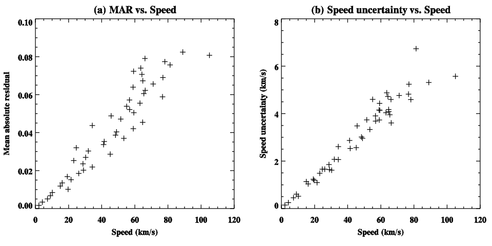
Figures \irefresiduald and e show the residual over time for the pixel with the smallest and largest final MAR respectively. The solid line shows the initial residual (zero velocity), and the dashed shows the residual at the final iteration. The velocity found for the pixel of figure \irefresiduald obviously satisfies the changes in brightness well over all time, since the final residual is close to zero. The solution is less satisfactory for the pixel of figure \irefresiduale. There is a clear linear relationship between the magnitude of the velocity at a given pixel and the MAR which is shown in figure \ireferrorsa. This figure shows, for a subset of 50 pixels, the MAR as a function of the speed at that pixel.
Inspection of the distribution of the MAR can show the effectiveness of the velocity field in describing the changes in brightness. The distribution of MAR for the final velocity solution, shown in figure \irefresidualc, varies greatly from pixel to pixel and is not smooth or coherent over large regions. This means that there are no large regions where the method is performing worse than for other regions. One exception to this is application of the method to large and complex active regions. In tests on active region data, we have noticed discrepancies in the velocity field where a coronal loop system crosses an underlying loop system. This is to be expected, since Equation \irefeqnlk1 tries to find a single velocity which is smoothly consistent with the local group of pixels, whereas a superimposed system of loops at different orientations suggests two or more velocities are needed (at two or more heights in the corona).
An estimate of errors in the method is difficult. In particular, error propagation from the original data, through the time normalisation process, and our implementation of the Lucas Kanade algorithm is not feasible. A bootstrapping approach to error estimation is required, but is not feasible to apply to all pixels since the bootstrapping estimate requires repeating the least-squares fit hundreds of times to gain meaningful statistics. We instead select a subset of pixels covering the full range of MAR, and apply the randomised-residual bootstrapping approach described by Byrne et al. 2013. For each pixel, we find a least-squares solution to Equation \irefeqnlk1 and calculate the residuals over time (as shown in figures \irefresiduald and e). These residuals are randomised in order, and added to the original of Equation —refeqnlk1. A least-squares solution is found, and the current and solutions recorded. This process is repeated 300 times, giving a distribution of solutions, with the spread based on the magnitude of the residuals. The standard deviation of the velocity distribution gives an error estimate on the resulting speed. Figure \ireferrorsb shows the speed uncertainty as a function of speed for a selection of 50 pixels. There is a clear linear relationship equating to a mean uncertainty of 6.5% on our speed estimates. This is just an indication of the uncertainties as dictated by the fitting residuals, and does not include biases introduced by choices of various method parameters such as the choice of wide kernel width in the time normalisation.
2.5 Computational efficiency
Using a standard desktop computer (3.7 GHz 6-Core Intel Core i5, with 32Gb memory), the whole process including reading in the data files, preprocessing, time normalisation, and the Lucas-Kanade algorithm, takes approximately 5 minutes. This is a factor of around 40 times faster than the implementation of Morgan and Hutton 2018, and enables rapid processing of multiple datasets for future studies. The Lucas-Kanade iterative process converges rapidly during the first two or three iterations, and terminates when the iteration counter reaches the set maximum number of iterations (). typically converges to a value of 25%. This value is likely related to the space and time derivatives being increasingly dominated by noise with increasing iteration.
3 Results
results
Applying the method to the 2019/11/06 193Å channel dataset results in the velocity field shown in figure \ireffig3a. As shown by Morgan and Hutton 2018, the method can be applied to all the higher signal channels of AIA (304, 171, 193, and 211Å), with differing results. For the sake of demonstrating the method, the 193Å channel is chosen here since it has a high signal, and is dominated by emission from coronal plasma thus the results can be interpreted firmly in terms of coronal velocity fields, with little ‘contamination’ from lower atmospheric layers. The most common pattern of the field distribution for this quiet Sun region is a network of distinct cells, approximately circular, and of typical diameter 50 to 100” (36 to 72Mm). The largest coherent cell is centered near ”, and has a diameter well over 100”. Flows tend to begin at the centers of the cells (red colours) and diverge towards the cell boundaries (blue). Another common pattern consists of long spines of converging or diverging flows. One example of a divergent spine is located near ”. Some cells show rotation of flow, such as the cell located at ”, or another small cell at ”.

Figure \ireffig3b shows the estimated speed given by the Lucas-Kanade algorithm. Maximum speeds are 40 km , with most areas with speeds at 20 km or less. The regions of brightest intensity in the 193Å channel tend to correspond to the higher speeds, and also to regions of flow divergence (cell centers), although this relationship is not consistent across the whole region. The boundaries between cells are narrow and distinct. That is, there are no broad regions of close to zero speed, and cells bound each other closely. We do not have information on the line-of-sight motion, and the method gives only the plane of sky velocities. Furthermore, the results must be dominated by the atmospheric layer, or the height formation of the observed emission. The 193Å channel has peak response near a temperature of 1.6MK, so is sensitive to the motions in the low corona.
3.1 Comparison to the photosphere
Figure \ireffig4a shows an AIA 1700Å image of the photospheric ultraviolet (UV) continuum. To create this image, we take 13 images taken every 10 minutes between 2019/11/06 13:00 to 15:00, apply image alignment so that every image is aligned to the 2019/11/06 14:00 image, then calculate an average image. Whilst the photosphere experiences rapid changes on small scales over a two hour period, the main bright network features, on spatial scales of tens of arcsecs, remain fairly consistent and stable over this period. Figure \ireffig4b shows the brightest features highlighted in green. The spatial scale of this distribution is consistent with the boundaries of the supergranular network.
We wish to compare this photospheric network with the topology of the coronal velocity field. In order to do this, we calculate a simplified representation of the complicated flow fields. Figure \ireffig4c shows the vector velocity field in black, and the blue and red lines represent certain regions where the direction of the flow field changes direction abruptly. The direction of the flow field at each pixel is given by the angle . The Sobel edge enhancement operator is applied to this angular image to give a value at each pixel: very high values are found at regions where the angle in velocity direction changes abruptly - both the red and blue lines in figure \ireffig4c correspond to high values. The red (blue) colours denote where these regions of abrupt angular change have positive (negative) divergence. The blue lines overlie regions where flows converge from surrounding areas (sinks), whilst the red lines overlie the points and corridors where flows diverge to surrounding areas (sources).

Figure \ireffig4d plots the bright photospheric UV network in green, with the simplified representation of the coronal velocity field in red and blue. From a visual comparison, it is obvious that there is correlation between the distribution of photospheric network and the coronal velocity field. In many places, the position of photospheric and coronal features agree closely, for example at ”. There is obviously much further depth that can be applied to this analysis - for example, a rigorous correlation analysis, and a comparison with other AIA channels. Whilst this paper is more concerned with presenting the method and preliminary results, this qualitative comparison suggests that the coronal velocity field is strongly linked to the magnetic field topology in the quiet Sun. In particular, it seems as if the red lines, or the coronal sources, are most strongly correlated with the bright photospheric network. These preliminary results are closely linked to the findings of Sheeley and Warren 2012, who found regions of clear cellular structures in AIA 193Å images, linked to the underlying distribution of supergranular boundaries.
3.2 Comparison to the previous method
Figure \ireffig5a shows the result of applying the new method to a disk centre region observed by the AIA 193Å channel between 2015/03/21 18:00 to 20:00, corresponding to the data used in Morgan and Hutton 2018. This region has more varied structure compared to the quiet coronal example shown in figure \ireffig3, with a small active region in the south-east, bounded to the west by a dark region, possibly a dark canopy region (Wang, Robbrecht, and Muglach 2011) or a small coronal hole. Figure \ireffig5b shows the result of appyling the Morgan and Hutton 2018 method to the same data. The two results are very similar across most of the region, with only small local differences in vector alignments and position. The new method shows a little more detail on smaller spatial scales, due to the old method’s approach to model the velocities as smooth local geometrical functions.

The left panel of figure \irefactiveregion shows more detail of the small active region in the south-east in the AIA 193Å channel. This image has been processed using the multiscale Gaussian normalisation process to enhance smaller-scale features such as active region loops (Morgan and Druckmüller 2014). The right panel shows the vector velocity field using the new method. Qualitatively, the agreement between the loops and structures extending outwards from the active region in the left image agrees well with the distribution of the velocity vectors in the right panel, which gives confidence that the method is indeed detecting and characterising coherent motions along magnetic structure. This type of direct comparison is difficult to make in the quiet Sun since the structure in the images is less clear, that is, it is difficult to see clear systems of large and distinct loops in the quiet Sun compared to active regions.

4 Summary
summary
A time normalisation process applied to a series of AIA observations near disk centre reveals continuous and ubiquitous faint motions. A new, efficient method for tracing these motions is described. Application to quiet Sun observations of 2019/11/06 in the AIA 193Å channel, dominated by hot coronal emission, gives speeds of 0-40 km , and a velocity map which reveals a network of coherent flow cells of typical diameters 50 to 100” (36 to 72Mm). Results are similar to a previous, more complicated, method.
If we assume that the PD must follow the coronal magnetic field, then tracing their motions must give the direction of the magnetic field. We believe that the vector velocity field of figure \ireffig3a may give an indication of the coronal magnetic structure, and gives support to previous studies showing that the magnetic field of the quiet corona has a similar cellular structure. This is supported also by the visual comparison between the coronal velocity field and the photospheric UV network of figure \ireffig4d, which from a visual comparison seem to be strongly correlated. A comparison of the characteristics of the velocity field from multiple AIA channels with the photospheric network, to related photospheric motions, and photospheric vector magnetograms, is an approach which we are adopting to develop the results in future work. Another potential avenue is to combine the velocity vector fields with Doppler information from spectrometers, thus gaining a simultaneous map of plane-of-sky and line-of-sight speeds. We also plan to compare velocity fields for several AIA channels at different formation heights in order to gain further insight into the quiet Sun magnetic topology.
The software for this method is written in the Interactive Data Language (IDL), and can be used on any suitable datacube of regular cadence. The software is released as a package for public use at https://github.com/HuwMorgan/TNOF.
Acknowledgments
We acknowledge STFC grant ST/S000518/1 to Aberystwyth University, and the excellent facilities and support of SuperComputing Wales. The AIA/SDO data used here is courtesy of NASA/SDO and the AIA science team.
References
- Byrne et al. (2013) Byrne, J.P., Long, D.M., Gallagher, P.T., Bloomfield, D.S., Maloney, S.A., McAteer, R.T.J., Morgan, H., Habbal, S.R.: 2013, Improved methods for determining the kinematics of coronal mass ejections and coronal waves. A&A 557, A96. DOI. ADS.
- Fisher and Welsch (2008) Fisher, G.H., Welsch, B.T.: 2008, FLCT: A Fast, Efficient Method for Performing Local Correlation Tracking. In: Howe, R., Komm, R.W., Balasubramaniam, K.S., Petrie, G.J.D. (eds.) Subsurface and Atmospheric Influences on Solar Activity, Astronomical Society of the Pacific Conference Series 383, 373. ADS.
- Lemen et al. (2011) Lemen, J.R., Title, A.M., Akin, D.J., Boerner, P.F., Chou, C., Drake, J.F., Duncan, D.W., Edwards, C.G., Friedlaender, F.M., Heyman, G.F., Hurlburt, N.E., Katz, N.L., Kushner, G.D., Levay, M., Lindgren, R.W., Mathur, D.P., McFeaters, E.L., Mitchell, S., Rehse, R.A., Schrijver, C.J., Springer, L.A., Stern, R.A., Tarbell, T.D., Wuelser, J.-P., Wolfson, C.J., Yanari, C., Bookbinder, J.A., Cheimets, P.N., Caldwell, D., Deluca, E.E., Gates, R., Golub, L., Park, S., Podgorski, W.A., Bush, R.I., Scherrer, P.H., Gummin, M.A., Smith, P., Auker, G., Jerram, P., Pool, P., Soufli, R., Windt, D.L., Beardsley, S., Clapp, M., Lang, J., Waltham, N.: 2011, The Atmospheric Imaging Assembly (AIA) on the Solar Dynamics Observatory (SDO). Sol. Phys., 172. DOI. ADS.
- Lucas et al. (1981) Lucas, B.D., Kanade, T., et al.: 1981, An iterative image registration technique with an application to stereo vision. In: Proceedings of the 7th International Joint Conference on Artificial Intelligence 2, 674. Vancouver. http://dl.acm.org/citation.cfm?id=1623264.1623280.
- Morgan and Druckmüller (2014) Morgan, H., Druckmüller, M.: 2014, Multi-Scale Gaussian Normalization for Solar Image Processing. Sol. Phys. 289, 2945. DOI. ADS.
- Morgan and Hutton (2018) Morgan, H., Hutton, J.: 2018, Ubiquitous and Continuous Propagating Disturbances in the Solar Corona. ApJ 853, 145. DOI. ADS.
- Morgan and Pickering (2019) Morgan, H., Pickering, J.: 2019, SITES: Solar Iterative Temperature Emission Solver for Differential Emission Measure Inversion of EUV Observations. Sol. Phys. 294, 135. DOI. ADS.
- Pesnell, Thompson, and Chamberlin (2012) Pesnell, W.D., Thompson, B.J., Chamberlin, P.C.: 2012, The Solar Dynamics Observatory (SDO). Sol. Phys. 275, 3. DOI. ADS.
- Sheeley and Warren (2012) Sheeley, J. N. R., Warren, H.P.: 2012, Coronal Cells. ApJ 749, 40. DOI. ADS.
- Starck, Murtagh, and Bijaoui (1998) Starck, J.-L., Murtagh, F., Bijaoui, A.: 1998, Image processing and data analysis. The multiscale approach. ADS.
- Stenborg et al. (2011) Stenborg, G., Marsch, E., Vourlidas, A., Howard, R., Baldwin, K.: 2011, A novel technique to measure intensity fluctuations in EUV images and to detect coronal sound waves nearby active regions. A&A 526, A58. DOI. ADS.
- Wang, Ofman, and Davila (2009) Wang, T.J., Ofman, L., Davila, J.M.: 2009, Propagating Slow Magnetoacoustic Waves in Coronal Loops Observed by Hinode/EIS. ApJ 696, 1448. DOI. ADS.
- Wang, Robbrecht, and Muglach (2011) Wang, Y.-M., Robbrecht, E., Muglach, K.: 2011, The Evolution of Dark Canopies Around Active Regions. ApJ 733, 20. DOI. ADS.