Chiral current in Floquet cavity-magnonics

Shi-fan Qi Affiliation: School of Physics, Zhejiang University, Hangzhou 310027, Zhejiang, China Jun Jing Email: jingjun@zju.edu.cn Affiliation: School of Physics, Zhejiang University, Hangzhou 310027, Zhejiang, China

August 11, 2026

Abstract

Floquet engineering can induce complex collective behaviour and interesting synthetic gauge-field in quantum systems through temporal modulation of system parameters by periodic drives. Using a Floquet drive on frequencies of the magnon modes, we realize a chiral state-transfer in a cavity-magnonic system. The time-reversal symmetry is broken in such a promising platform for coherent information processing. In particular, the photon mode is adiabatically eliminated in the large-detuning regime and the magnon modes under conditional longitudinal drives can be indirectly coupled to each other with a phase-modulated interaction. The effective Hamiltonian is then used to generate chiral currents in a circular loop, whose dynamics is evaluated to measure the symmetry of the system Hamiltonian. Beyond the dynamics limited in the manifold with a fixed number of excitations, our protocol applies to the continuous-variable systems with arbitrary states. Also it is found to be robust against the systematic errors in the photon-magnon coupling strength and Kerr nonlinearity.

I Introduction

With unique properties observed in experiments such as large tunability and long coherent-time, the magnon can be used as information carrier in a broad variety of hybrid systems Rameshti et al. 2021; Lachance-Quirion et al. 2019; Li et al. 2020; Yuan et al. 2022. Found to be directly or effectively coupled to microwave photon Soykal and Flatté 2010a; Soykal and Flatté 2010b; Tabuchi et al. 2014; Zhang et al. 2014; Wang et al. 2018; Shen et al. 2021, superconducting qubit Lachance-Quirion et al. 2020; Tabuchi et al. 2015; Qi and Jing 2022a; Yan and Jing 2021, spin-emitter Neuman et al. 2020; Qi and Jing 2021a, and phonon Zhang et al. 2016; Li et al. 2018a; Qi and Jing 2021b; Li et al. 2021; Hatanaka et al. 2022; Potts et al. 2021; Shen et al. 2022, the magnon modes provide novel applications in quantum computing Ladd et al. 2010, quantum communication Reiserer and Rempe 2015, and quantum sensing Degen et al. 2017. Fundamentally, the coupling between magnon and other types of mode motivates a number of insights, e.g., the indirect two-body flip-flop interaction of magnons for Rabi oscillation, which is symmetrical to time and parity. Moreover, Floquet engineering has been applied to a cavity electromagnonic system Xu et al. 2020. It could support more flexible and interesting applications based on the complex-valued hopping, such as generating chiral transfers of the quasiparticles of spin waves as a highly promising bosonic platform.

Chirality has played an important role in the photon and phonon systems Lodahl et al. 2017; Zhu et al. 2018. Optical lattice could be used to simulate the chirality in magnetic materials Sørensen et al. 2005. In the platform of superconducting qubits Liu et al. 2020, spin chirality arises from the three-body interactions. The chirality operator of three spins is $\hat{O}=\vec{\sigma}_{1}\cdot(\vec{\sigma}_{2}\times\vec{\sigma}_{3})$ , where $\vec{\sigma}_{j}\equiv(\sigma^{x}_{j},\sigma^{y}_{j},\sigma^{z}_{j})$ is the Pauli vector for the $j$ th spin particle. It is straightforward to verify that $\hat{O}$ breaks both the time reversal symmetry $\mathcal{T}$ (replacing $\vec{\sigma}_{j}$ by $-\vec{\sigma}_{j}$ ) and the parity symmetry $\mathcal{P}$ (exchanging $\vec{\sigma}_{j}$ with $\vec{\sigma}_{k}$ ) but conserves the $\mathcal{PT}$ symmetry Liu et al. 2020. The dynamics of the spins driven by $\hat{O}$ features a chiral evolution, i.e., $|s_{1}s_{2}s_{3}\rangle\to$ $|s_{2}s_{3}s_{1}\rangle\to$ $|s_{3}s_{1}s_{2}\rangle$ , where $s_{j}=0$ (spin down) or $1$ (spin up) Cai and Wang 2021. In parallel to the protocol in the superconducting qubits, we propose to generate a chiral transfer of an arbitrary bosonic state in the Floquet cavity-magnonic system Xu et al. 2020. Here the system-Hamiltonian symmetry is described by a nonvanishing chiral current operator.

According to the Floquet theory Shirley 1965; Goldman and Dalibard 2014; Bukov et al. 2015; Petiziol et al. 2021, the propagator $U(t)$ induced by a time-dependent Hamiltonian $H(t)=H(t+T)$ with a period $T$ can be expressed by $U(t)=U_{F}(t)\exp(-iH^{\prime}t)$ , where $U_{F}(t)$ is also periodic with $T$ . As a time-independent Hermitian operator, $H^{\prime}=U^{\dagger}_{F}(t)H(t)U_{F}(t)-iU^{\dagger}_{F}(t)\dot{U}_{F}(t)$ can be understood as the system Hamiltonian in the frame defined by $U_{F}(t)$ . Floquet engineering by fast periodic modulation over the characteristic frequencies of a quantum system is a major control approach to the long-time dynamics of the system Goldman and Dalibard 2014; Shao et al. 2017; Wang et al. 2016a; Li et al. 2019, where the effective Hamiltonian can be synthesized through designing proper drives. Floquet engineering has been applied to quantum switch Wu et al. 2018, chiral ground state current Roushan1 et al. 2017, quantum simulation Kyriienko and Sørensen 2018, and perfect state transfer Wang et al. 2019; Liu et al. 2020; Li et al. 2018b in superconducting qubits. Also it found a very wide application in quantum gas systems Eckardt 2017; Weitenberg and Simonet 2021 to reveal many interesting physics.

In this work, we apply the Floquet engineering to a hybrid photon-magnon system in which three single-crystal yttrium iron garnet (YIG) spheres are placed inside a microwave cavity. The uniform bias magnetic field excites the Kittel mode in the YIG spheres and establishes a strong photon-magnon coupling. In the large detuning regime, the common photon mode can be adiabatically eliminated with the standard perturbation theory Garziano et al. 2016; Ma and Law 2015; Kaufman et al. 2020 or the high-order Fermi golden rule Combescot 2001. By periodically modulating over the three magnon modes with well-controlled intensities, frequencies, and phases, we can obtain an effective time-reversal symmetry broken Hamiltonian Koch et al. 2010, that ensures chiral magnon currents Roushan1 et al. 2017 of arbitrary states with a state-independent period. In contrast to the protocols based on the superconducting qubits Roushan1 et al. 2017; Wang et al. 2019; Liu et al. 2020, our protocol is not constrained in a manifold of a fixed number of excitations and is capable to transfer versatile states such as Fock state, coherent state, Schrödinger cat state, and even two-body entangled states in a chiral way. The magnon Fock state can be generated by the magnon blockade Xie et al. 2020; Liu et al. 2019. A magnonic cat state was proposed in Ref. Kounalakis et al. 2022. And more magnonic-state preparation protocols have been collected in a recent review Yuan et al. 2022.

The rest part of this work is structured as follows. In Sec. II, we introduce the quantum model for a Floquet cavity-magnonic system and then derive an effective Hamiltonian to generate a perfect chiral state transfer amongst magnons. Clockwise and anticlockwise transfers of various states and chiral currents to measure the symmetry of the system Hamiltonian are presented in Sec. III.1 and Sec. III.2, respectively. State-transfer fidelity under the magnon damping and the systematic errors arise from the photon-magnon coupling strength and the Kerr effects are discussed in Sec. IV.1 and Sec. IV.2, respectively. The whole work is summarized in Sec. V.

II Model

Consider a hybrid quantum model consists of a microwave cavity coupled to $N$ YIG spheres in their Kittle modes Xu et al. 2020; Wang et al. 2018; Wang et al. 2016b. The model Hamiltonian reads

H=\omega_{a}a^{\dagger}a+\omega_{m}\sum_{k=1}^{N}m^{\dagger}_{k}m_{k}+g_{am}\sum_{k=1}^{N}\left(am^{\dagger}_{k}+a^{\dagger}m_{k}\right),

(1)

where $a$ $(a^{\dagger})$ and $m_{k}$ $(m^{\dagger}_{k})$ are the annihilation (creation) operators of the photon and the $k$ th magnon modes, respectively. $\omega_{a}$ and $\omega_{m}$ are their respective transition frequencies. $g_{am}$ is the single-excitation coupling strength between photon and magnon modes, which is much larger than their decay rates and much smaller than their detuning $|\omega_{a}-\omega_{m}|$ in the dispersive regime. Counter-rotating interaction between photon and magnons is omitted under the rotating-wave approximation (RWA), as justified in Appendix A.

When one focuses on the state exchange within any pair of magnon modes, it is instructive to show that the photon mode could be adiabatically eliminated by the second-order perturbation Garziano et al. 2016. The subsystem Hamiltonian associated with the $k$ th and $j$ th magnon modes and the photon mode can be written as $H^{kj}_{0}+H^{kj}_{I}$ , where

	$\displaystyle H^{kj}_{0}$	$\displaystyle=\omega_{a}a^{\dagger}a+\omega_{m}\left(m_{k}^{\dagger}m_{k}+m_{j}^{\dagger}m_{j}\right),$		(2)
	$\displaystyle H^{kj}_{I}$	$\displaystyle=g_{am}\left[a\left(m^{\dagger}_{k}+m^{\dagger}_{j}\right)+a^{\dagger}\left(m_{k}+m_{j}\right)\right]$		(2)

indicating the unperturbed and perturbation Hamiltonians, respectively. To the second order in the perturbation Hamiltonian, the effective coupling strength $g_{pq}$ between any pair of eigenstates $|p\rangle$ and $|q\rangle$ of $H^{kj}_{0}$ in Eq. (2) is given by

g_{pq}=\sum_{w\neq p,q}\frac{\langle q|H^{kj}_{I}|w\rangle\langle w|H^{kj}_{I}|p\rangle}{E_{p}-E_{w}},

(3)

where $E_{w}$ is the eigenenergy of an intermediate eigenstate $|w\rangle$ , namely, $H^{kj}_{0}|w\rangle=E_{w}|w\rangle$ . Note that the large detuning condition $\omega_{m}\neq\omega_{a}$ lifts the degeneracy of $H^{kj}_{0}$ . Due to the excitation conservation in both Eqs. (1) and (2), $g_{pq}$ can be probed as the transition rate between $|p\rangle=|n_{k}n_{a}n_{j}\rangle\equiv|n_{k}\rangle|n_{a}\rangle|n_{j}\rangle$ and $|q\rangle=|(n_{k}-1)n_{a}(n_{j}+1)\rangle$ in a subspace with a fixed number of excitations $M=n_{k}+n_{a}+n_{j}$ , where the subscript indicates the mode and $n_{k}$ , $n_{a}$ , and $n_{j}$ are arbitrary nonnegative integers. By Eqs. (2) and (3), the leading contribution for $|n_{k}n_{a}n_{j}\rangle\to|(n_{k}-1)n_{a}(n_{j}+1)\rangle$ comes from two physical paths, i.e., $|n_{k}n_{a}n_{j}\rangle\to|(n_{k}-1)(n_{a}+1)n_{j}\rangle\to|(n_{k}-1)n_{a}(n_{j}+1)\rangle$ and $|n_{k}n_{a}n_{j}\rangle\to|n_{k}(n_{a}-1)(n_{j}+1)\rangle\to|(n_{k}-1)n_{a}(n_{j}+1)\rangle$ . Then in this subspace we have

g_{n_{k}n_{j}}=\sqrt{n_{k}(n_{j}+1)}\frac{g^{2}_{am}}{\omega_{m}-\omega_{a}}=g\sqrt{n_{k}(n_{j}+1)}.

(4)

Note $m_{k}|n_{k}\rangle=\sqrt{n_{k}}|n_{k}-1\rangle$ and $m_{j}^{\dagger}|n_{j}\rangle=\sqrt{n_{j}+1}|n_{j}+1\rangle$ . The effective Hamiltonian for this pair of magnon modes in their full space Qi and Jing 2021b can thus be written as

H_{kj}=g\left(m_{k}m^{\dagger}_{j}+m^{\dagger}_{k}m_{j}\right),\quad g\equiv\frac{g^{2}_{am}}{\omega_{m}-\omega_{a}}.

(5)

The preceding derivation as well as the construction of the effective Hamiltonian applies to any indirect magnon-magnon interaction mediated by the common photon mode. In the dispersive regime, the Hamiltonian for the whole model in Eq. (1) can therefore be written as

H=g\sum_{k<j}^{N}\left(m_{k}m^{\dagger}_{j}+m^{\dagger}_{k}m_{j}\right).

(6)

We apply the periodic signals by Floquet driving Xu et al. 2020; Liu et al. 2020 featured with the intensity $\Delta$ , the frequency $\omega$ , and the local phases $\phi_{k}$ , to the model Hamiltonian and obtain

	$\displaystyle H(t)$	$\displaystyle=\Delta\sum_{k=1}^{N}\cos(\omega t+\phi_{k})m^{\dagger}_{k}m_{k}$		(7)
		$\displaystyle+g\sum_{k<j}^{N}\left(m_{k}m^{\dagger}_{j}+m^{\dagger}_{k}m_{j}\right).$		(7)

In the rotating frame with respect to

	$\displaystyle U_{0}(t)$	$\displaystyle=\exp\left[i\int^{t}_{0}ds\Delta\sum_{k=1}^{N}\cos(\omega s+\phi_{k})m^{\dagger}_{k}m_{k}\right]$		(8)
		$\displaystyle=\exp\left\{i\sum^{N}_{k=1}\frac{\Delta}{\omega}\left[\sin(\omega t+\phi_{k})-\sin\phi_{k}\right]m^{\dagger}_{k}m_{k}\right\},$		(8)

we have

	$\displaystyle H_{I}(t)$	$\displaystyle=U_{0}(t)H(t)U^{\dagger}_{0}(t)-iU_{0}(t)\dot{U}^{\dagger}_{0}(t)$		(9)
	$\displaystyle=$	$\displaystyle\sum_{k<j}^{N}g_{kj}\exp\left[if_{kj}\sin(\omega t+\alpha_{kj})\right]m_{k}^{\dagger}m_{j}+{\rm H.c.},$		(9)

where

		$\displaystyle g_{kj}=ge^{-i\beta_{kj}},\quad\beta_{kj}\equiv\frac{\Delta}{\omega}(\sin\phi_{k}-\sin\phi_{j}),$
		$\displaystyle f_{kj}=\frac{2\Delta}{\omega}\sin\left(\frac{\phi_{j}-\phi_{k}}{2}\right),$
		$\displaystyle\alpha_{kj}\equiv\tan^{-1}\left(\frac{\sin\phi_{k}-\sin\phi_{j}}{\cos\phi_{k}-\cos\phi_{j}}\right).$

According to the Jacobi-Anger expansion $e^{ix\sin y}=\sum_{n=-\infty}^{n=+\infty}J_{n}(x)e^{iny}$ , where $J_{n}$ is the $n$ th Bessel function of the first kind, one can obtain

H_{I}(t)=H_{0}+\sum_{n=1}^{\infty}\left(H_{n}e^{in\omega t}+H_{-n}e^{-in\omega t}\right),

(10)

with

	$\displaystyle H_{0}$	$\displaystyle=\sum_{k<j}^{N}J_{0}(f_{kj})\left(g_{kj}m^{\dagger}_{k}m_{j}+g^{*}_{kj}m_{k}m_{j}^{\dagger}\right),$		(11)
	$\displaystyle H_{n}$	$\displaystyle=\sum_{k<j}^{N}J_{n}(f_{kj})e^{in\alpha_{kj}}\left[g_{kj}m^{\dagger}_{k}m_{j}+(-1)^{n}g_{kj}^{*}m_{k}m_{j}^{\dagger}\right],$		(11)

and $H_{-n}=H_{n}^{*}$ . Therefore up to the order of $\mathcal{O}(1/\omega)$ , the Floquet-driving Hamiltonian (7) can be written as

H_{\rm eff}=H_{0}+H_{\rm eff}^{(2)}=H_{0}+\sum^{\infty}_{n=1}\frac{1}{n\omega}\left[H_{n},H_{-n}\right].

(12)

We have several remarks for $H_{\rm eff}$ . (a) The zeroth-order coupling-strength between the $k$ th and $j$ th magnons is $g_{kj}J_{0}(f_{kj})$ , which can be tuned by the ratio of the driving intensity and frequency $\Delta/\omega$ and the phase difference between the local driving signals $\phi_{k}-\phi_{j}$ . (b) When $N=2$ , the leading-order correction by the commutator $[H_{n},H_{-n}]$ vanishes and then the dynamics of magnons becomes a Rabi oscillation with a frequency fully determined by $f_{kj}$ . (c) When $N>2$ , the leading-order correction can be written as

H_{\rm eff}^{(2)}=\sum_{k<j}\left(g^{(2)}_{kj}e^{i\alpha_{kj}}m_{k}^{\dagger}m_{j}+h.c.\right),

(13)

where the second-order coupling strength is

g^{(2)}_{kj}\sim\frac{g^{2}}{\omega}\sum_{k_{1}\neq k,j}\left[\sum^{\infty}_{n=1}\frac{J_{n}(f_{kk_{1}})J_{n}(f_{k_{1}j})}{n}\right],

(14)

with $k_{1}$ indicating the other magnon modes rather than $k$ and $j$ in the whole system.

The third and even higher orders of terms can be analyzed with the James’ effective-Hamiltonian method Shao et al. 2017. The nonvanishing third-order terms in the effective Hamiltonian can be obtained by

	$\displaystyle H^{(3)}_{kj}$	$\displaystyle=\sum_{l=m+n}\frac{1}{(n+m)\omega^{2}}\left[H_{n},\left[H_{m},H_{-l}\right]\right]$		(15)
		$\displaystyle=\sum_{k<j}\left(g^{(3)}_{kj}e^{i\alpha_{kj}}m_{k}^{\dagger}m_{j}+H.c.\right),$		(15)

where the third-order coupling strength $g^{(3)}_{kj}$ is about

\sim\frac{g^{3}}{\omega^{2}}\sum_{k_{1}\neq k,k_{2}\neq j}\left[\sum_{l=m+n}\frac{J_{n}(f_{kk_{1}})J_{m}(f_{k_{1}k_{2}})J_{l}(f_{k_{2}j})}{n+m}\right].

(16)

Therefore the third and even higher orders of corrections can be safely omitted in the dispersive regime $g\ll\omega$ .

Chiral state-transfer (as described in Fig. 1) could manifest when $N=3$ by setting $\phi_{j}=2\pi j/3$ , $j=1,2,3$ , which are uniformly distributed in the range of $[0,2\pi]$ . In this case, the magnitude of the ratio factor $f_{kj}$ becomes independent of the magnon pair, i.e., $f_{12}=f_{13}=f_{23}=\sqrt{3}\Delta/\omega\equiv f$ . The relevant quantum phases are found to be $\beta_{12}=f$ , $\beta_{23}=-f/2$ , $\beta_{13}=f/2$ ; and $\alpha_{12}=\pi/2$ , $\alpha_{13}=5\pi/6$ , $\alpha_{23}=7\pi/6$ , i.e., $\alpha_{kj}=(k+j)\pi/3-\pi/2$ . Then using $H_{n}$ in Eq. (11), the second-order term in the effective Hamiltonian (12) turns out to be

H^{(2)}_{\rm eff}=-ig_{\rm eff}\sum_{j=k+1}\left(e^{-i\beta_{kj}}m_{k}^{\dagger}m_{j}-e^{i\beta_{kj}}m_{k}m^{\dagger}_{j}\right).

(17)

Note if $k=3$ , then $j=1$ , and

g_{\rm eff}=g_{\rm eff}(f)=\frac{2g^{2}}{\omega}\sum_{n=1}^{\infty}\frac{J^{2}_{n}(f)}{n}\sin\left(\frac{n\pi}{3}\right).

(18)

Consequently, the effective Hamiltonian in Eq. (12) can be expressed by an coefficient matrix,

H_{\rm eff}=[m^{\dagger}_{1},m^{\dagger}_{2},m^{\dagger}_{3}]\begin{bmatrix}0&G^{*}e^{-if}&Ge^{-if/2}\\ Ge^{if}&0&G^{*}e^{if/2}\\ G^{*}e^{if/2}&Ge^{-if/2}&0\end{bmatrix}\begin{bmatrix}m_{1}\\ m_{2}\\ m_{3}\end{bmatrix},

(19)

where $G=gJ_{0}(f)+ig_{\rm eff}$ is the effective coupling strength. Using $\tan\phi\equiv g_{\rm eff}/[gJ_{0}(f)]$ , the Hamiltonian has a more compact form,

H_{\rm eff}=|G|[m^{\dagger}_{1},m^{\dagger}_{2},m^{\dagger}_{3}]\begin{bmatrix}0&e^{i\phi_{12}}&e^{-i\phi_{31}}\\ e^{-i\phi_{12}}&0&e^{i\phi_{23}}\\ e^{i\phi_{31}}&e^{-i\phi_{23}}&0\end{bmatrix}\begin{bmatrix}m_{1}\\ m_{2}\\ m_{3}\end{bmatrix},

(20)

where $\phi_{12}=-\phi-f$ , $\phi_{23}=-\phi+f/2$ , and $\phi_{31}=-\phi+f/2$ . The eigenvalues of the coefficient matrix satisfy $E^{3}-3E-2\cos\Phi=0$ , where $\Phi\equiv\phi_{12}+\phi_{23}+\phi_{31}=-3\phi$ is defined as the closed-loop phase up to $2n\pi$ with $n$ an integer. The system dynamics is then found to be relevant to the driving intensity and frequency rather than solely determined by the ratio factor $f$ . $\Phi$ is thus regarded as the synthetic magnetic flux. It is gauge-invariant by noting that in our model the three YIGs form a closed loop and the accumulated phase of the state-current (either chiral or not) has to be single-valued when going around this loop. $\Phi=0$ or $\pi$ corresponds to the absence of the Floquet engineering. Then the evolution of the magnons is symmetrical when one of the magnons (say mode- $1$ ) is prepared at the target state and the rest two are in the same states. The quantum state propagates from mode- $1$ to mode- $2$ and mode- $3$ simultaneously and then back to mode- $1$ . This pattern repeats itself with no indication of any preferred circulation direction.

III Numerical simulation of Chiral currents

III.1 Chiral state transfer

Refer to caption — Figure 1: (a) and (b): Diagrams of the chiral state transfers in the magnons along the clockwise and anticlockwise circles, respectively. (c): Diagram of the chiral entanglement transfer along the clockwise direction, where two yellow nodes connected by a solid line represent the two entangled magnons and the blue node represents a separable magnon.

With a Hamiltonian similar to Eq. (20), that is obtained by the tunneling-term modulation Roushan1 et al. 2017 rather than the longitudinal Floquet driving, the time-reversal symmetry broken was distinguished when the loop phase $\Phi=\pm\pi/2$ . This idea can be generalized to realize a chiral state-transfer in our continuous-variable system for arbitrary target states.

Due to Eq. (19), $\Phi=\pi/2$ yields $G=ig_{\rm eff}$ under the condition of $J_{0}(f)=0$ . It renders that $f=\sqrt{3}\Delta/\omega=2.4048$ . Consequently, $J_{1}(f)=0.5192$ , $J_{2}(f)=0.4318$ , $J_{3}(f)=0.1990$ , $J_{4}(f)=0.0647$ , $J_{5}(f)=0.0164$ , $J_{6}(f)=0.0034$ . The Hamiltonian becomes

H_{\rm eff}=ig_{\rm eff}[m^{\dagger}_{1},m^{\dagger}_{2},m^{\dagger}_{3}]\begin{bmatrix}0&-e^{-if}&e^{-if/2}\\ e^{if}&0&-e^{if/2}\\ -e^{if/2}&e^{-if/2}&0\end{bmatrix}\begin{bmatrix}m_{1}\\ m_{2}\\ m_{3}\end{bmatrix}.

(21)

Note when $N\geq 4$ , $f_{kj}$ ’s are not the same in magnitude. Consequently, the zeroth-order time-reversal symmetry Hamiltonian $H_{0}$ in Eq. (11) remains in any case. It is then hard to observe a perfect chiral state-transfer. The canonical transformation in the Heisenberg picture induced by Eq. (21) can be written as

\begin{bmatrix}m_{1}(t)\\ m_{2}(t)\\ m_{3}(t)\end{bmatrix}=T(t)\begin{bmatrix}m_{1}(0)\\ m_{2}(0)\\ m_{3}(0)\end{bmatrix}

(22)

with

T(t)=\frac{1}{3}\begin{bmatrix}x(t)&e^{-if}y(t)&e^{-\frac{if}{2}}z(t)\\ e^{if}z(t)&x(t)&e^{\frac{if}{2}}y(t)\\ e^{\frac{if}{2}}y(t)&e^{-\frac{if}{2}}z(t)&x(t)\end{bmatrix},

(23)

where

$\displaystyle x(t)$	$\displaystyle=1+2\cos\left(\sqrt{3}g_{\rm eff}t\right),$	(24)
$\displaystyle y(t)$	$\displaystyle=1-2\cos\left(\sqrt{3}g_{\rm eff}t+\frac{\pi}{3}\right),$
$\displaystyle z(t)$	$\displaystyle=1-2\cos\left(\sqrt{3}g_{\rm eff}t-\frac{\pi}{3}\right).$

With respect to the time-evolved operator, it is interesting to find that $m_{3}(t)=m_{1}(0)$ and $m_{2}(t)=m_{3}(0)$ when $t=(2\pi/3+2n\pi)/(\sqrt{3}g_{\rm eff})$ ; $m_{2}(t)=m_{1}(0)$ and $m_{3}(t)=m_{2}(0)$ when $t=(4\pi/3+2n\pi)/(\sqrt{3}g_{\rm eff})$ ; and $m_{j}(t)=m_{j}(0)$ when $t=2n\pi/(\sqrt{3}g_{\rm eff})$ with $n$ an integer. This transfer is exactly described by the clockwise rotation $m_{1}\to m_{3}\to m_{2}\to m_{1}$ in Fig. 1(a), corresponding to a chiral evolution in the Schrödinger picture, i.e., $|\varphi_{1}\varphi_{2}\varphi_{3}\rangle\to$ $|\varphi_{2}\varphi_{3}\varphi_{1}\rangle\to$ $|\varphi_{3}\varphi_{1}\varphi_{2}\rangle$ , where $\varphi_{j}$ is arbitrary for the $j$ th mode.

The state-transfer fidelity in the Schrödinger picture can be measured by the time-dependent state population $P_{j}(t)$ , $j=1,2,3$ , which can be defined by

P_{j}(t)=\sum_{C_{n}\neq 0}\left|\left\langle\varphi(t)\Big|\frac{(m^{\dagger}_{j})^{n}}{\sqrt{n!}}\Big|000\right\rangle\right|^{2}.

(25)

It describes the overlap between the target state and the $j$ th mode’s state without regarding the influence from local dynamical phases Qi and Jing 2022b. Here the initial state of the magnons is assumed to be $|\varphi(0)\rangle=\sum_{n}C_{n}|n00\rangle\equiv\sum_{n}C_{n}|n\rangle_{1}|0\rangle_{2}|0\rangle_{3}$ with the normalized coefficients $C_{n}$ , i.e., the first magnon is prepared as an arbitrary target state and the other two are in their ground states. The dynamics of the magnons is analytically determined by Eq. (22) or numerically calculated by the Floquet-driving Hamiltonian in Eq. (7).

For $|\varphi(0)\rangle=|100\rangle$ , we have

|\varphi(t)\rangle=\frac{1}{3}\left[x(t)|100\rangle+e^{-if}z(t)|010\rangle+e^{\frac{-if}{2}}y(t)|001\rangle\right].

(26)

While for an arbitrary superposed state

|\varphi(0)\rangle=\sum_{n}C_{n}|n00\rangle=\sum_{n}\frac{C_{n}}{\sqrt{n!}}\left[m^{\dagger}_{1}(0)\right]^{n}|000\rangle,

(27)

the time-evolved state can be written as

|\varphi(t)\rangle=\sum_{n}\frac{C_{n}}{\sqrt{n!}}\left[\sum_{j}m^{\dagger}_{1}(0)T_{j1}^{\dagger}(t)\right]^{n}|000\rangle.

(28)

Then due to Eqs. (22) and (23), we have $\varphi(t_{3})=\sum_{n}C_{n}|00n\rangle$ at the desired time $t_{3}=2\pi/(3\sqrt{3}g_{\rm eff})$ and $\varphi(t_{2})=\sum_{n}C_{n}|0n0\rangle$ at $t_{2}=4\pi/(3\sqrt{3}g_{\rm eff})$ , up to certain local phases. By virtue of Eq. (25), we have $P_{1}=\sum_{n}x^{2n}(t)|C_{n}|^{2}/9^{n}$ , $P_{2}=\sum_{n}z^{2n}(t)|C_{n}|^{2}/9^{n}$ , and $P_{3}=\sum_{n}y^{2n}(t)|C_{n}|^{2}/9^{n}$ . During the state transfer of $m_{1}\to m_{3}$ , the population of $m_{2}$ achieve the side peak value at $t=(\pi/3+2n\pi)/(\sqrt{3}g_{\rm eff})$ , which is undesired for $m_{1}\to m_{3}$ yet cannot be under control. In particular, $P_{2}^{\rm max}=\sum_{n}|C_{n}|^{2}/9^{n}$ at those moments. Similarly, when $t=(\pi+2n\pi)/(\sqrt{3}g_{\rm eff})$ and $t=(5\pi/3+2n\pi)/(\sqrt{3}g_{\rm eff})$ , $P_{1}$ and $P_{3}$ are expected to achieve their side peak values in the middle of $m_{3}\to m_{2}$ and $m_{2}\to m_{1}$ , respectively. In addition, one can even transfer a mixed state by $\rho(t)=\sum_{j}p_{j}|\varphi(t)\rangle_{jj}\langle\varphi(t)|$ based on Eq. (28).

Figure 2 is used to verify the time evolutions of the state populations $P_{j}(t)$ by the Floquet-driving Hamiltonian (7) under the chiral condition of $J_{0}(f)=0$ in comparison with those by the effective Hamiltonian (21) or the canonical transformation (22). It is found that the analytical results (lines with markers) do match with their numerical counterparts (lines without markers) for the normalized time evolution. The periodic dynamics is determined once $g$ is fixed.

In Fig. 3, the chiral transfer protocol is applied to Fock state, Glauber coherent state $|\beta\rangle$ , cat state $(|\zeta\rangle+|-\zeta\rangle)/\sqrt{2+2e^{-2|\zeta|^{2}}}$ with $|\zeta\rangle$ a coherent state, and thermal state $\rho=\sum_{n}p_{n}|n\rangle\langle n|$ with the Fock-state occupation $p_{n}=(\bar{n})^{n}/(1+\bar{n})^{n+1}$ and the average excitation number $\bar{n}$ . Periodically all the state populations approach unit in sequence indicating a perfect clockwise transfer amongst $m_{1}$ , $m_{2}$ , and $m_{3}$ . It is interesting to find that the side peak for the Fock state is more significant than the other states that occupy the vacuum state. It is caused by the distinction between the side peak and initial values $P_{2}^{\rm max}-P_{2}(0)=\sum_{n}(1/9)^{n}|C_{n}|^{2}-|C_{0}|^{2}$ . In Fig. 3(a), (b) and (c), the distinctions are about $0.11$ , $0.05$ and $0.01$ , respectively. Figures 2 and 3 demonstrate that the Floquet-driving Hamiltonian in Eq. (21) under the chiral conditions $J_{0}(f)=0$ and $\phi_{j}=2\pi j/3$ would ensure a high-fidelity chiral state-transfer for arbitrary target states. And the transfer period is irrespective to the chosen initial state.

By setting $\phi_{1}=2\pi/3$ , $\phi_{2}=2\pi$ , and $\phi_{3}=4\pi/3$ , which is an alternative uniform distribution in the range of $[0,2\pi]$ , the coefficient matrix in Eq. (19) becomes

\begin{bmatrix}0&Ge^{-if/2}&G^{*}e^{-if}\\ G^{*}e^{if/2}&0&G^{*}e^{if/2}\\ Ge^{if}&Ge^{if/2}&0\end{bmatrix}

(29)

where $G=gJ_{0}(f)-ig_{\rm eff}$ . That induces the synthetic magnetic flux with $\Phi=-\pi/2$ . It amounts to exchange the magnon mode- $2$ and $3$ , giving rise to the anticlockwise rotation shown in Fig 1(b). Then the effective Hamiltonian in Eq. (21) is modified to

H_{\rm eff}=ig_{\rm eff}[m^{\dagger}_{1},m^{\dagger}_{2},m^{\dagger}_{3}]\begin{bmatrix}0&e^{-if/2}&-e^{-if}\\ -e^{if/2}&0&-e^{-if/2}\\ e^{if}&e^{if/2}&0\end{bmatrix}\begin{bmatrix}m_{1}\\ m_{2}\\ m_{3}\end{bmatrix}

(30)

Through a canonical transformation similar to Eq. (22), one can easily analyse the anticlockwise state-transfer. For example, the time-dependent state $|\varphi(t)\rangle$ in Eq. (26) for the single-excitation state becomes

|\varphi(t)\rangle=\frac{1}{3}\left[x(t)|100\rangle+e^{\frac{-if}{2}}y(t)|010\rangle+e^{-if}z(t)|001\rangle\right],

(31)

where $x(t)$ , $y(t)$ , and $z(t)$ are given by Eq. (24). The numerical results for various states are provided in Fig. 4, exhibiting the opposite chirality to Fig. 3. During the anticlockwise state-transfer $m_{1}\to m_{2}\to m_{3}$ , all the magnon modes achieve a nearly unit fidelity in a periodical sequence. Anticlockwise chiral state-transfer also applies to arbitrary states.

If any two magnons in our model could be prepared as an entangled state and the third one is separably initialized as the ground state, we can demonstrate a high-fidelity chiral transfer for the pairwise quantum entanglement [see Fig. 1(c)]. In particular, we consider that mode- $1$ and mode- $3$ are prepared as a double-excitation Bell state $(|00\rangle+|11\rangle)/\sqrt{2}$ or a NOON state $(|0N\rangle+|N0\rangle)/\sqrt{2}$ under the clockwise-transfer condition, i.e., $\Phi=\pi/2$ .

It is well known that the concurrence could be used as a sufficient and necessary entanglement criterion for any bipartite system in pure state and any bipartite two-state system. According to its definition Wootters 1998 for a two-qubit system $AB$ , $C=\max\{0,\lambda_{1}-\lambda_{2}-\lambda_{3}-\lambda_{4}\}$ , where $\lambda_{j}$ are the square root of the eigenvalues of $\rho_{AB}(\sigma^{A}_{y}\otimes\sigma^{B}_{y})\rho^{*}_{AB}(\sigma^{A}_{y}\otimes\sigma^{B}_{y})$ in the decreasing order. For a pure state $a|11\rangle+b|10\rangle+c|01\rangle+d|00\rangle$ with normalized coefficients, its concurrence can be easily derived as $C=2|bc-ad|$ .

Inspired by the expression for the pure state, we here employ a modified concurrence to measure the chiral-transfer of the entangled state in our model. If the initial state is the Bell state $(|00\rangle+|11\rangle)/\sqrt{2}$ , then the concurrence between mode- $j$ and mode- $k$ is defined as $C_{jk}(t)=2|\langle\varphi(t)|00\rangle_{jk}||\langle\varphi(t)|11\rangle_{jk}|$ ; and if the target state is initially chosen as the NOON state $(|0N\rangle+|N0\rangle)/\sqrt{2}$ , then $C_{jk}(t)=2|\langle\varphi(t)|0N\rangle_{jk}||\langle\varphi(t)|N0\rangle_{jk}|$ . These definitions amount to the original occurrence under the perfect state transfer and become sufficient but not necessary for the entangled states during the time evolution, which is calculated with the Floquet-driving Hamiltonian (7).

In Fig. 5, the blue solid lines, the red dot-dashed lines, and the yellow dotted lines represent the concurrences for mode- $1$ and mode- $3$ , mode- $3$ and mode- $2$ , and mode- $2$ and mode- $1$ , respectively. It is found that both the double-excitation Bell state and the NOON state could be transferred in a chiral way along the magnon triangle. At the same desired moments for the faithful state transfer, one can observe a nearly perfect entanglement transfer. Comparing Fig. 5(a) and Fig. 5(b), it is found that the undesired magnon pair obtains a lower probability of entanglement generation in transferring NOON state than Bell state. The side peaks of the Bell state $(|00\rangle+|11\rangle)/\sqrt{2}$ are dominant because its constituent $|00\rangle$ does not participate in the time evolution. Our model then widens the application range of the chiral state-transfer.

III.2 Chiral current

Chiral current is an effective measure for the symmetry of the system Hamiltonian in condensed matter systems, which can be probed by measuring the energy spectrum under varying synthetic field $\Phi$ Roushan1 et al. 2017. Using the definition in Ref. Roushan1 et al. 2017, we can consider the continuity equation for each magnon mode, e.g., $\partial_{t}\hat{n}_{k}=I_{\rm in}-I_{\rm out}$ , where $\hat{n}_{k}\equiv m^{\dagger}_{k}m_{k}$ is the occupation operator of the $k$ th magnon mode and $I_{\rm in}$ ( $I_{\rm out}$ ) represents the input (output) current with respect to mode- $k$ . Under the necessary condition for the clockwise transfer in Fig. 1(a), i.e., $\phi_{j}=2\pi j/3$ , $j=1,2,3$ , we have three equations of motion:

$\displaystyle\partial_{t}\hat{n}_{1}$	$\displaystyle=I_{12}-I_{31}=i\left[H_{\rm eff},\hat{n}_{1}\right],$	(32)
$\displaystyle\partial_{t}\hat{n}_{2}$	$\displaystyle=I_{23}-I_{12}=i\left[H_{\rm eff},\hat{n}_{2}\right],$
$\displaystyle\partial_{t}\hat{n}_{3}$	$\displaystyle=I_{31}-I_{23}=i\left[H_{\rm eff},\hat{n}_{3}\right],$

where $H_{\rm eff}$ is the effective Hamiltonian in Eq. (19) or Eq. (20) and $I_{jk}$ represents the current from mode- $j$ to mode- $k$ . Then we have

	$\displaystyle I_{12}=iGe^{if}m_{1}m^{\dagger}_{2}-iG^{*}e^{-if}m^{\dagger}_{1}m_{2},$		(33)
	$\displaystyle I_{31}=-iG^{*}e^{-if/2}m_{1}m^{\dagger}_{3}+iGe^{if/2}m^{\dagger}_{1}m_{3},$
	$\displaystyle I_{23}=iGe^{-if/2}m_{2}m^{\dagger}_{3}-iG^{*}e^{if/2}m^{\dagger}_{2}m_{3}.$

Normalized by the coupling-strength $|G|$ of $H_{\rm eff}$ , the effective current operator from mode- $j$ to mode- $k$ can be defined as

\hat{I}_{kj}=ie^{-i\phi_{kj}}m_{k}m^{\dagger}_{j}-ie^{i\phi_{kj}}m^{\dagger}_{k}m_{j}.

(34)

Accordingly, the circle current operator is defined as $\hat{I}=\hat{I}_{12}+\hat{I}_{23}+\hat{I}_{31}$ . It is straightforward to find that the circle current operator is an integral of motion because it commutates with the effective Hamiltonian, i.e., $[H_{\rm eff},\hat{I}]=0$ . It means that the expectation value of $\langle\hat{I}\rangle$ can not be used to measure the time-reversal symmetry of our model.

We have known that the magnon system has a symmetrical evolution for a synthetic magnetic flux $\Phi=0$ or $\Phi=\pi$ under the effective Hamiltonian in Eq. (20). In this case, arbitrary state of mode- $1$ simultaneously propagates to mode- $2$ and mode- $3$ and periodically goes back to mode- $1$ . Consequently, the current $\langle\hat{I}_{23}\rangle$ from mode- $2$ to mode- $3$ vanishes. A nonzero current $\langle\hat{I}_{23}\rangle$ appears when the time-reversal symmetry is broken when $\Phi\neq 0,\pi$ and becomes maximum when $\Phi=\pm\pi/2$ . We check the condition of $\Phi=\pi/2$ under $\phi_{j}=2\pi j/3$ . Using $|\varphi(t)\rangle$ in Eq. (26) with the initial Fock state $|100\rangle$ , it is found that

\langle\hat{I}_{23}(t)\rangle=\frac{4}{9}\left[2\cos^{2}\left(\sqrt{3}g_{\rm eff}t\right)-\cos\left(\sqrt{3}g_{\rm eff}t\right)-1\right].

(35)

The maximal value is achieved as $\langle\hat{I}_{23}^{\rm max}\rangle=8/9$ when $\sqrt{3}g_{\rm eff}t=\pi+2n\pi$ . Given an arbitrary state in Eq. (28), we have

\langle\hat{I}_{23}^{\rm max}\rangle=\frac{8}{9}\sum_{n}nC^{2}_{n}=\frac{8}{9}\bar{n},

(36)

where $\bar{n}$ is the average excitation number of the state. For a coherent state $|\beta\rangle$ , $\bar{n}=|\beta|^{2}$ and for a cat state $(|\zeta\rangle+|-\zeta\rangle)/\sqrt{2+2e^{-2|\zeta|^{2}}}$ , $\bar{n}=|\zeta|^{2}[1-\exp(-2|\zeta|^{2})]/[1+\exp(-2|\zeta|^{2})]$ . Then the expectation value of $\langle\hat{I}_{23}(t)\rangle$ is effective to measure the time-reversal or parity-reversal symmetry of the system Hamiltonian.

The preceding analysis is consistent with the numerical simulation in Fig. 6 about $\langle\hat{I}_{23}^{\rm max}\rangle$ as a function of the close-loop phase or the synthetic magnetic field $\Phi$ . It is found that the maximal current vanishes when $\Phi=0$ and $\Phi=\pi$ . It can be understood that at these points, the system Hamiltonian becomes real that cannot break the time-reversal symmetry. Otherwise, any finite $\Phi$ breaks the symmetry and leads to the chiral currents. It is interesting to find in Fig. 6(a) that the maximal currents for the Fock state $|n=1\rangle$ and the coherent state with $\beta=1$ are equivalent to each other. Both of them equal to $0.89\approx 8/9$ at the peak point $\Phi=\pi/2$ . They are larger than the cat state with $\zeta=1$ , whose peak value is $0.68$ . A larger average excitation number yields a larger $\langle\hat{I}_{23}^{\rm max}\rangle$ with the same $\Phi$ . This result is also supported by Fig. 6(b), in which a monotonic pattern appears with increasing $n$ .

IV Fidelity analysis

IV.1 Fidelity analysis under magnon damping

Taking account the magnon damping into consideration, we can study the chiral state-transfer fidelity in a standard open-quantum-system framework. In general, the full Hamiltonian including the environments can be written as

H_{\rm tot}=H(t)+\sum_{k=1}^{3}\left(m_{k}B_{k}^{\dagger}+m_{k}^{\dagger}B_{k}\right),

(37)

where $H(t)$ is the Floquet-driving Hamiltonian (7) with $N=3$ and $B_{k}=\sum_{j}g_{kj}a^{\dagger}_{kj}e^{-i\omega_{kj}t}$ is a collective environmental operator. $\omega_{kj}$ is the eigenfrequency for the $j$ th field mode in the $k$ th environment and $g_{kj}$ is its coupling strength with the $k$ th magnon mode. Under the Markovian approximation and tracing out the degrees of freedom of the external environments (assumed to be at the vacuum state), we arrive at the master equation Breuer and Petruccione 2022 for the density-matrix operator $\rho(t)$ for the magnon system:

\dot{\rho}(t)=-i\left[H(t),\rho(t)\right]+\kappa\sum_{k=1}^{3}\mathcal{L}[m_{k}]\rho(t),\\

(38)

where $\kappa$ is the damping rate. The dissipative superoperator $\mathcal{L}$ is in a Lindblad form,

\mathcal{L}[o]\rho\equiv\frac{1}{2}\left(2o\rho o^{\dagger}-o^{\dagger}o\rho-\rho o^{\dagger}o\right),

(39)

where $o=m_{1},m_{2},m_{3}$ are the decay operators.

In Fig. 7(a), one can observe that the open-system dynamics under $\kappa/g=0.001$ is very close to the closed-system result in Fig. 3(a). And in Fig. 7(b), it is found that at least one round of chiral transfer presents when $\kappa/g=0.01$ . It is thus required that the effective coupling strength $g$ is about two orders higher than the damping rate in magnitude. For YIG spheres of a typical size about $250$ $\mu$ m in recent experiments Tabuchi et al. 2014; Tabuchi et al. 2015; Lachance-Quirion et al. 2020, the coupling strength $g$ was found to be in the order of $1\sim 10$ MHz and the damping rate $\kappa\sim 1$ MHz. Then our protocol could become practical in a near future by increasing the strength of the magnetic dipole interaction to the order of $100$ MHz Lachance-Quirion et al. 2019.

Alternatively, we can apply the external quantum control, such as the dynamical decoupling method Viola and Lloyd 1998, to our system to neutralize the magnon damping effects. The system coherence can then be saved by the $\pi$ -pulses exerted on the magnons. It is known that

e^{i\int_{\tau_{n}}^{\tau_{n+1}}dt\Omega(t)m_{k}^{\dagger}m_{k}}m_{k}e^{-i\int_{\tau_{n}}^{\tau_{n+1}}dt\Omega(t)m_{k}^{\dagger}m_{k}}=-m_{k}

(40)

as long as $\int_{\tau_{n}}^{\tau_{n+1}}dt\Omega(t)=\pi$ . In the ideal situation for dynamical decoupling, $\Omega(t)=\pi/(\tau_{n+1}-\tau_{n})\delta(t-s)$ with $s\in(\tau_{n},\tau_{n+1})$ . Thus it could reverse the decoherence dynamics induced by the unwanted terms $m_{k}B_{k}^{\dagger}+H.c.$ in Eq. (37), but does not change the effective Hamiltonian in our protocol.

IV.2 Fidelity under systematic errors

Our protocol based on Eq. (1) has been discussed under the ideal condition that all the coupling strengths $g_{am}$ between photon and magnon modes are the same in magnitude. While in practice Zhang et al. 2014; Lachance-Quirion et al. 2019, they are associated with the individual locations of the YIG spheres in the cavity. We first consider the systematic errors raised by the nonequal coupling strengths. In particular, it is assumed that $g_{am}^{(1)}=g_{am}$ , $g_{am}^{(2)}=g_{am}(1+\delta)$ , and $g_{am}^{(3)}=g_{am}(1-\delta)$ , where the superscript $j\in\{1,2,3\}$ marks the coupling strength between the common photon and the $j$ th magnon and $\delta$ is used to estimate the magnitude of the relative error. With $N=3$ , the system Hamiltonian in Eq. (1) is then rewritten as

$\displaystyle H$	$\displaystyle=\omega_{a}a^{\dagger}a+\omega_{m}\sum_{k=1}^{3}m^{\dagger}_{k}m_{k}+g_{am}\left(am^{\dagger}_{1}+a^{\dagger}m_{1}\right)$	(41)
	$\displaystyle+g_{am}(1+\delta)\left(am^{\dagger}_{2}+a^{\dagger}m_{2}\right)$
	$\displaystyle+g_{am}(1-\delta)\left(am^{\dagger}_{3}+a^{\dagger}m_{3}\right).$

Under the conditions that $\phi_{j}=2\pi j/3$ and $J_{0}(f)=0$ for the clockwise chiral transfer, the effective Hamiltonian in Eq. (21) is modified by changing the coefficient matrix to be

ig_{\rm eff}\begin{bmatrix}0&-(1-\delta^{2})e^{if}&(1+\delta)e^{if/2}\\ (1-\delta^{2})e^{-if}&0&-(1-\delta)e^{-if/2}\\ -(1+\delta)e^{-if/2}&(1-\delta)e^{if/2}&0\end{bmatrix}.

(42)

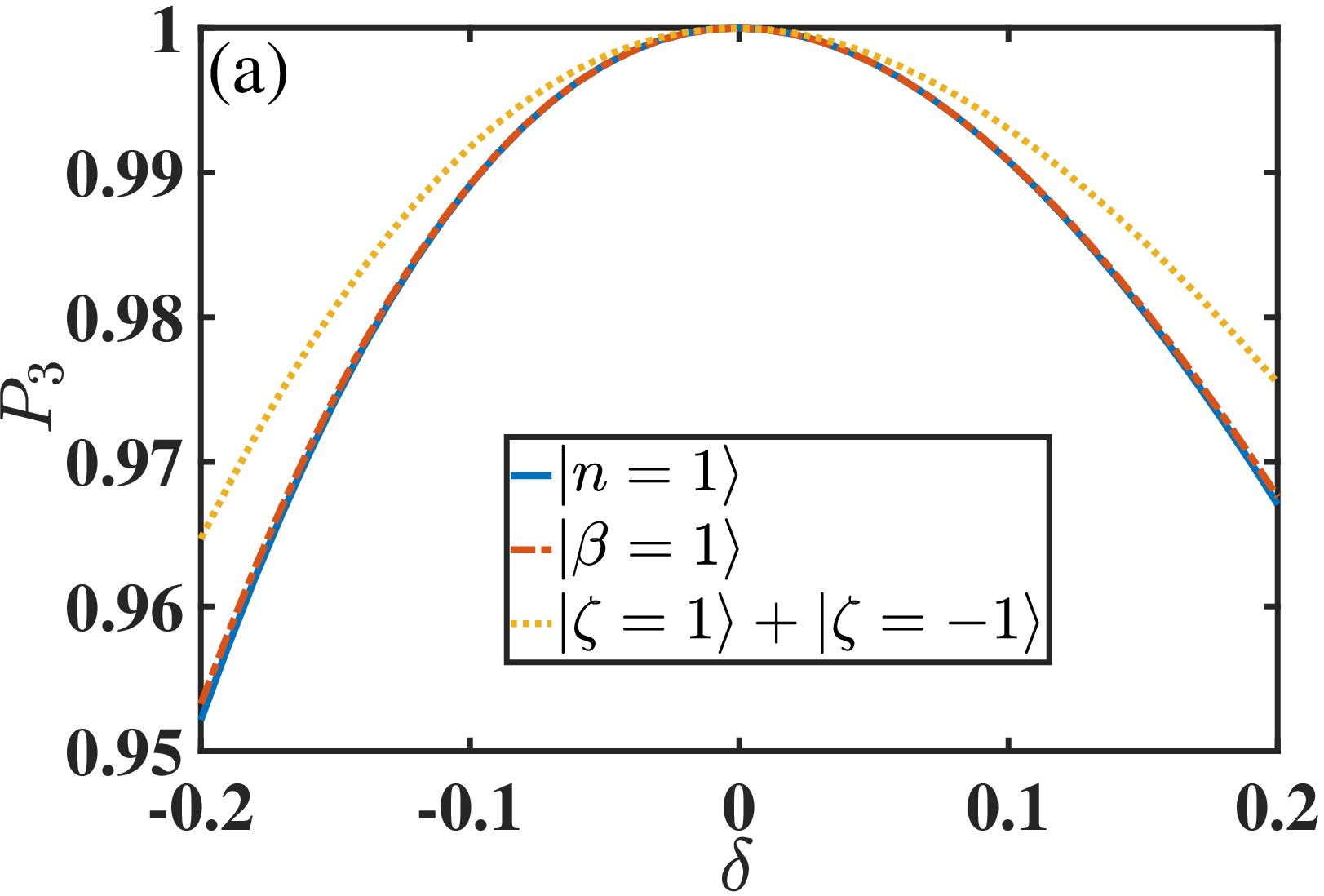
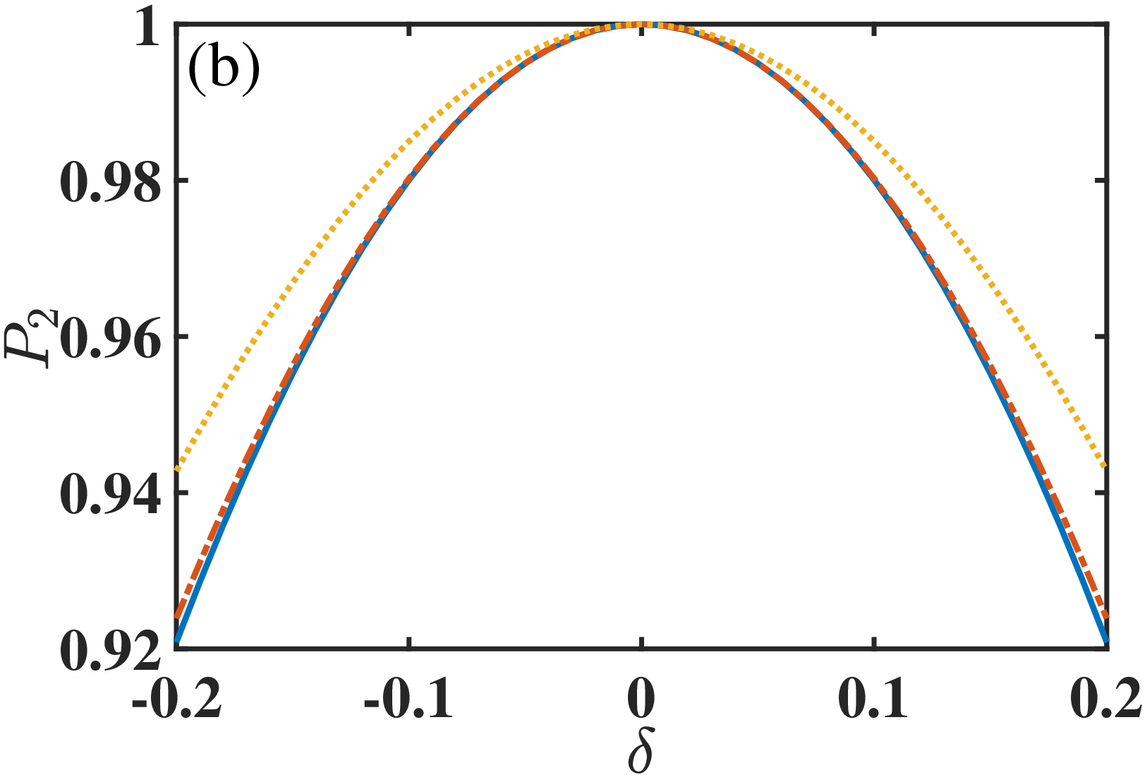
In Fig. 8, we present the sensitivity of the state populations [see Eq. (25)] to the error $\delta$ for $g_{ma}$ at the desired moments for the chiral state-transfer obtained by Eq. (24). It is found that the robustness of our protocol against the systematic errors becomes weaker with a larger average population. The cat state with $\zeta=1$ is found to be more robust in comparison with the Fock state $|n=1\rangle$ and the coherent state with $\beta=1$ . For all of them, both transferred populations of mode- $2$ and mode- $3$ could be maintained above $0.98$ in the presence of about $10\%$ errors or fluctuations in the photon-magnon coupling strength.

Another systematic error in our model is associated with the nonlinearity in the expansion of the YIG crystal or the dipolar anisotropy energy quadratic in the magnon numbers, which is parameterized with the Kerr coefficient $K$ . When the excitation number in the spin wave is much smaller than the total number of spins in YIG sphere, the system Hamiltonian in Eq. (6) can be modified to Wang et al. 2018; Wang et al. 2016b

\tilde{H}_{\rm Kerr}=g\sum_{k<j}\left(m_{k}m^{\dagger}_{j}+m^{\dagger}_{k}m_{j}\right)+K\sum_{k}\left(m^{\dagger}_{k}m_{k}\right)^{2}.

(43)

The Kerr coefficient $K/2\pi\approx 6.4\times 10^{-9}$ Hz, which is much smaller than the effective coupling strength $g$ . Given the timescale we considered in the preceding chiral dynamics, we can safely apply our model in such a hybrid photon-magnon system when the number of the excited spins $\langle m^{\dagger}_{k}m_{k}\rangle$ is less than $10^{6}$ .

V Conclusion

In summary, we have proposed a chiral state-transfer proposal in a Floquet cavity-magnonic system, which consists of a microwave cavity coupled to three YIG spheres in their Kittle mode. The three magnon modes constitute a triangle loop of mutual interaction through eliminating the photon mode in a state-resolved way. The Floquet driving with desired parameters forms complex-valued hopping of magnons, that generates a tunable synthetic magnetic flux. Our results open a path toward simulation of a time-reversal-broken continuous-variable system, yielding the chiral transfer for arbitrary states and even quantum entanglement. It is beyond the limitation of fixed excitation numbers. We evaluate the chiral current to measure the symmetry of the system Hamiltonian. We discuss the feasibility of the chiral transfer in the presence of magnon damping. The stability of our proposal is also tested with respect to the systematic errors in the coupling strength and the nonlinear terms in the system. Our work in pursuit of the quantum chiral state transfer provides an interesting application in cavity magnonics as a promising hybrid platform for control over the emerging phases.

Our theory can be straightforwardly generalized to arbitrary continuous-variable systems that could be indirectly coupled to each other by a common mediator. For example, one can replace our magnon modes with microwave photon modes in superconducting circuit with a much reduced ratio of decoherence and coupling strength Niemczyk et al. 2010. In addition, although our protocol has no direct relation with topological variables, the anomalous edge states, and the bulk-edge correspondence in the momentum space, we expect that the edge state Cai and Wang 2021; Roushan1 et al. 2017; Rudner et al. 2013 can arise from the cavity-magnonic system of a larger size under Floquet engineering. It will bring extra interesting physics.

Acknowledgments

We acknowledge financial support from the National Science Foundation of China (Grants No. 11974311 and No. U1801661).

Appendix A RWA in Hamiltonian (1)

This appendix contributes to verifying that it is valid to apply the rotating-wave approximation in the model Hamiltonian (1). Without loss of generality, it is instructive to focus on the state exchange (Rabi oscillation) between two magnons mediated by a common photon mode as what we concerned in Eq. (2). Including the counter-rotating terms, the Hamiltonian reads

H=\omega_{a}a^{\dagger}a+\omega_{m}\sum_{k=1}^{2}m^{\dagger}_{k}m_{k}+g_{am}\left(a+a^{\dagger}\right)\sum_{k=1}^{2}\left(m^{\dagger}_{k}+m_{k}\right).

(44)

And it becomes

H_{\rm rwa}=\omega_{a}a^{\dagger}a+\omega_{m}\sum_{k=1}^{2}m^{\dagger}_{k}m_{k}+g_{am}\sum_{k=1}^{2}\left(am^{\dagger}_{k}+a^{\dagger}m_{k}\right)

(45)

under RWA.

To demonstrate the effect from the counter-rotating terms in a practical cavity-magnon system Wang et al. 2018; Wang et al. 2016b on Rabi oscillation of the two modes, we plot their population dynamics using the total Hamiltonian in Eq. (44) and that under RWA in Eq. (45). One can find that in Fig. 9(a), the difference between $H$ and $H_{\rm rwa}$ is not significant when $\omega_{m}=100g_{am}$ ; and in Fig. 9(b) it becomes ignorable when $\omega_{m}=200g_{am}$ . Thus we are sure that it is not necessary to include the counter-rotating terms since $g_{am}\ll\Delta=\omega_{a}-\omega_{m}$ is in the strong instead of ultrastrong regimes.

Note the counter-rotating terms does not constitute an obstacle for our state-resolved method Qi and Jing 2021b to eliminate the mediator [see from Eq. (2) to Eq. (5)]. We can still obtain an effective Hamiltonian for the magnons as in Eq. (5), and it is little different from the current result in the dispersive regime of $g_{am}$ .

References

Rameshti et al. (2021) B. Z. Rameshti, S. V. Kusminskiy, J. A. Haigh, K. Usami, D. Lachance-Quirion, Y. Nakamura, C.-M. Hu, H. X. Tang, G. E. Bauer, and Y. M. Blanter, Cavity magnonics, arxiv: 2106. 09312v1 (2021).
Lachance-Quirion et al. (2019) D. Lachance-Quirion, Y. Tabuchi, A. Gloppe, K. Usami, and Y. Nakamura, Hybrid quantum systems based on magnonics, Appl. Phys. Express 12, 070101 (2019).
Li et al. (2020) Y. Li, W. Zhang, V. Tyberkevych, W. K. Kwok, and V. Novosad, Hybrid magnonics: physics, circuits, and applications for coherent information processing, J. Appl. Phys. 128, 130902 (2020).
Yuan et al. (2022) H. Yuan, Y. Cao, A. Kamra, R. A. Duine, and P. Yan, Quantum magnonics: When magnon spintronics meets quantum information science, Phys. Rep. 965, 1 (2022).
Soykal and Flatté (2010a) O. O. Soykal and M. E. Flatté, Strong field interactions between a nanomagnet and a photonic cavity, Phys. Rev. Lett. 104, 077202 (2010a).
Soykal and Flatté (2010b) O. O. Soykal and M. E. Flatté, Size dependence of strong coupling between nanomagnets and photonic cavities, Phys. Rev. B 82, 104413 (2010b).
Tabuchi et al. (2014) Y. Tabuchi, S. Ishino, T. Ishikawa, R. Yamazaki, K. Usami, and Y. Nakamura, Hybridizing ferromagnetic magnons and microwave photons in the quantum limit, Phys. Rev. Lett. 113, 083603 (2014).
Zhang et al. (2014) X. Zhang, C.-L. Zou, L. Jiang, and H. X. Tang, Strongly coupled magnons and cavity microwave photons, Phys. Rev. Lett. 113, 156401 (2014).
Wang et al. (2018) Y.-P. Wang, G.-Q. Zhang, D. Zhang, T.-F. Li, C.-M. Hu, and J. Q. You, Bistability of cavity magnon polaritons, Phys. Rev. Lett. 120, 057202 (2018).
Shen et al. (2021) R.-C. Shen, Y.-P. Wang, J. Li, S.-Y. Zhu, G. S. Agarwal, and J. Q. You, Long-time memory and ternary logic gate using a multistable cavity magnonic system, Phys. Rev. Lett. 127, 183202 (2021).
Lachance-Quirion et al. (2020) D. Lachance-Quirion, S. Piotr Wolski, Y. Tabuchi, S. Kono, K. Usami, and Y. Nakamura, Entanglement-based single-shot detection of a single magnon with a superconducting qubit, Science 367, 425 (2020).
Tabuchi et al. (2015) Y. Tabuchi, S. Ishino, A. Noguchi, T. Ishikawa, R. Yamazaki, K. Usami, and Y. Nakamura, Coherent coupling between a ferromagnetic magnon and a superconducting qubit, Science 349, 405 (2015).
Qi and Jing (2022a) S.-f. Qi and J. Jing, Generation of bell and greenberger-horne-zeilinger states from a hybrid qubit-photon-magnon system, Phys. Rev. A 105, 022624 (2022a).
Yan and Jing (2021) J.-s. Yan and J. Jing, External-level assisted cooling by measurement, Phys. Rev. A 104, 063105 (2021).
Neuman et al. (2020) T. c. v. Neuman, D. S. Wang, and P. Narang, Nanomagnonic cavities for strong spin-magnon coupling and magnon-mediated spin-spin interactions, Phys. Rev. Lett. 125, 247702 (2020).
Qi and Jing (2021a) S.-f. Qi and J. Jing, Magnon-mediated quantum battery under systematic errors, Phys. Rev. A 104, 032606 (2021a).
Zhang et al. (2016) X. Zhang, C.-L. Zou, L. Jiang, and H. Tang, Cavity magnonmechanics, Sci. Adv. 2, e1501286 (2016).
Li et al. (2018a) J. Li, S.-Y. Zhu, and G. S. Agarwal, Magnon-photon-phonon entanglement in cavity magnomechanics, Phys. Rev. Lett. 121, 203601 (2018a).
Qi and Jing (2021b) S.-f. Qi and J. Jing, Magnon-assisted photon-phonon conversion in the presence of structured environments, Phys. Rev. A 103, 043704 (2021b).
Li et al. (2021) J. Li, Y.-P. Wang, W.-J. Wu, S.-Y. Zhu, and J. You, Quantum network with magnonic and mechanical nodes, PRX Quant. 2, 040344 (2021).
Hatanaka et al. (2022) D. Hatanaka, M. Asano, H. Okamoto, Y. Kunihashi, H. Sanada, and H. Yamaguchi, On-chip coherent transduction between magnons and acoustic phonons in cavity magnomechanics, Phys. Rev. Appl. 17, 034024 (2022).
Potts et al. (2021) C. A. Potts, E. Varga, V. A. S. V. Bittencourt, S. V. Kusminskiy, and J. P. Davis, Dynamical backaction magnomechanics, Phys. Rev. X 11, 031053 (2021).
Shen et al. (2022) R.-C. Shen, J. Li, Z.-y. Fan, Y.-P. Wang, and J. You, Mechanical bistability in kerr-modeified cavity magnomechanics, arxiv: 2206. 14588 (2022).
Ladd et al. (2010) T. D. Ladd, F. Jelezko, R. Laflamme, Y. Nakamura, C. Monroe, and J. L. O’Brien, Quantum computers, Nature (London) 464, 45 (2010).
Reiserer and Rempe (2015) A. Reiserer and G. Rempe, Cavity-based quantum networks with single atoms and optical photons, Rev. Mod. Phys. 87, 1379 (2015).
Degen et al. (2017) C. L. Degen, F. Reinhard, and P. Cappellaro, Quantum sensing, Rev. Mod. Phys. 89, 035002 (2017).
Xu et al. (2020) J. Xu, C. Zhong, X. Han, D. Jin, L. Jiang, and X. Zhang, Floquet cavity electromagnonics, Phys. Rev. Lett. 125, 237201 (2020).
Lodahl et al. (2017) P. Lodahl, S. Mahmoodian, S. Stobbe, A. Rauschenbeutel, P. Schneeweiss, J. Volz, H. Pichler, and P. Zoller, Chiral quantum optics, Nature 541, 473 (2017).
Zhu et al. (2018) H. Zhu, J. Yi, M.-Y. Li, J. Xiao, L. Zhang, C.-W. Yang, R. A. Kaindl, L.-J. Li, Y. Wang, and X. Zhang, Observation of chiral phonons, Science 359, 579 (2018).
Sørensen et al. (2005) A. S. Sørensen, E. Demler, and M. D. Lukin, Fractional quantum hall states of atoms in optical lattices, Phys. Rev. Lett. 94, 086803 (2005).
Liu et al. (2020) W. Liu, W. Feng, W. Ren, D.-W. Wang, and H. Wang, Synthesizing three-body interaction of spin chirality with superconducting qubits, Appl. Phys. Lett. 116, 114001 (2020).
Cai and Wang (2021) H. Cai and D.-W. Wang, Topological phases of quantized light, Nat. Sci. Rev. 8, nwaa196 (2021).
Shirley (1965) J. H. Shirley, Solution of the schrödinger equation with a hamiltonian periodic in time, Phys. Rev. 138, B979 (1965).
Goldman and Dalibard (2014) N. Goldman and J. Dalibard, Periodically driven quantum systems: Effective hamiltonians and engineered gauge fields, Phys. Rev. X 4, 031027 (2014).
Bukov et al. (2015) M. Bukov, L. D’Alessio, and A. Polkovnikov, Universal high-frequency behavior of periodically driven system: from dynamical stabilization to floquet engineering, Adv. in Phys. 64, 139 (2015).
Petiziol et al. (2021) F. Petiziol, M. Sameti, S. Carretta, S. Wimberger, and F. Mintert, Quantum simulation of three-body interactions in weakly driven quantum systems, Phys. Rev. Lett. 126, 250504 (2021).
Shao et al. (2017) W. Shao, C. Wu, and X.-L. Feng, Generalized james’ effective hamiltonian method, Phys. Rev. A 95, 032124 (2017).
Wang et al. (2016a) D.-W. Wang, H. Cai, R.-B. Liu, and M. O. Scully, Mesoscopic superposition states generated by synthetic spin-orbit interaction in fock-state lattices, Phys. Rev. Lett. 116, 220502 (2016a).
Li et al. (2019) H. Li, H. Cai, J. Xu, V. V. Yakovlev, Y. Yang, and D.-W. Wang, Quantum photonic transistor controlled by an atom in a floquet cavity-qed system, Opt. Express 27, 6946 (2019).
Wu et al. (2018) Y. Wu, L.-P. Yang, M. Gong, Y. Zheng, H. Deng, Z. Yan, Y. Zhao, K. Huang, A. D. Castellano, W. J. Munro, K. Nemoto, D.-N. Zheng, C. Sun, Y.-x. Liu, X. Zhu, and L. Lu, An efficient and compact switch for quantum circuits, npj. Quantum Inf. 4, 50 (2018).
Roushan1 et al. (2017) P. Roushan1, C. Neill, A. Megrant, Y. Chen, R. Babbush, R. Barends, B. Campbell, Z. Chen, B. Chiaro, A. Dunsworth, A. Fowler, E. Jeffrey, J. Kelly, E. Lucero, J. Mutus, P. ÓMalley, M. Neeley, C. Quintana, D. Sank, A. Vainsencher, J. Wenner, T. White, E. Kapit, H. Neven, and J. Martinis, Chiral ground-state currents of interacting photons in a synthetic magnetic field, Nat. Phys. 13, 146 (2017).
Kyriienko and Sørensen (2018) O. Kyriienko and A. S. Sørensen, Floquet quantum simulation with superconducting qubits, Phys. Rev. Appl. 9, 064029 (2018).
Wang et al. (2019) D.-W. Wang, C. Song, W. Feng, and et al., Synthesis of antisymmetric spin exchange interaction and chiral spin clusters in superconducting circuits, Nat. Phys. 15, 382 (2019).
Li et al. (2018b) X. Li, Y. Ma, J. Han, T. Chen, Y. Xu, W. Cai, H. Wang, Y. Song, Z.-Y. Xue, Z.-q. Yin, and L. Sun, Perfect quantum state transfer in a superconducting qubit chain with parametrically tunable couplings, Phys. Rev. Appl. 10, 054009 (2018b).
Eckardt (2017) A. Eckardt, Colloquium: Atomic quantum gases in periodically driven optical lattices, Rev. Mod. Phys. 89, 011004 (2017).
Weitenberg and Simonet (2021) C. Weitenberg and J. Simonet, Tailoring quantum gases by floquet engineering, Nat. Phys. 17, 1342 (2021).
Garziano et al. (2016) L. Garziano, V. Macrì, R. Stassi, O. Di Stefano, F. Nori, and S. Savasta, One photon can simultaneously excite two or more atoms, Phys. Rev. Lett. 117, 043601 (2016).
Ma and Law (2015) K. K. W. Ma and C. K. Law, Three-photon resonance and adiabatic passage in the large-detuning rabi model, Phys. Rev. A 92, 023842 (2015).
Kaufman et al. (2020) B. Kaufman, T. Rozgonyi, P. Marquetand, and T. Weinacht, Adiabatic elimination in strong-field light-matter coupling, Phys. Rev. A 102, 063117 (2020).
Combescot (2001) M. Combescot, On the generalized golden rule for transition probabilities, J. Phys. A: Math. Gen. 34, 6087 (2001).
Koch et al. (2010) J. Koch, A. A. Houck, K. L. Hur, and S. M. Girvin, Time-reversal-symmetry breaking in circuit-qed-based photon lattices, Phys. Rev. A 82, 043811 (2010).
Xie et al. (2020) J.-k. Xie, S.-l. Ma, and F.-l. Li, Quantum-interference-enhanced magnon blockade in an yttrium-iron-garnet sphere coupled to superconducting circuits, Phys. Rev. A 101, 042331 (2020).
Liu et al. (2019) Z.-X. Liu, H. Xiong, and Y. Wu, Magnon blockade in a hybrid ferromagnet-superconductor quantum system, Phys. Rev. B 100, 134421 (2019).
Kounalakis et al. (2022) M. Kounalakis, G. E. W. Bauer, and Y. M. Blanter, Analog quantum control of magnonic cat states on a chip by a superconducting qubit, Phys. Rev. Lett. 129, 037205 (2022).
Wang et al. (2016b) Y.-P. Wang, G.-Q. Zhang, D. Zhang, X.-Q. Luo, W. Xiong, S.-P. Wang, T.-F. Li, C.-M. Hu, and J. Q. You, Magnon kerr effect in a strongly coupled cavity-magnon system, Phys. Rev. B 94, 224410 (2016b).
Qi and Jing (2022b) S.-f. Qi and J. Jing, Accelerated adiabatic passage in cavity magnomechanics, Phys. Rev. A 105, 053710 (2022b).
Wootters (1998) W. K. Wootters, Entanglement of formation of an arbitrary state of two qubits, Phys. Rev. Lett. 80, 2245 (1998).
Breuer and Petruccione (2022) H.-P. Breuer and F. Petruccione, The theory of open quantum systems, Oxford University Press, Oxford (2022).
Viola and Lloyd (1998) L. Viola and S. Lloyd, Dynamical suppression of decoherence in two-state quantum systems, Phys. Rev. A 58, 2733 (1998).
Niemczyk et al. (2010) T. Niemczyk, F. Deppe, H. Huebl, E. P. Menzel, F. Hocke, M. J. Schwarz, J. J. Garciaripoll, D. Zueco, T. Hömmer, and E. Solano, Circuit quantum electrodynamics in the ultrastrong-coupling regime, Nat. Phys. 6, 772 (2010).
Rudner et al. (2013) M. S. Rudner, N. H. Lindner, E. Berg, and M. Levin, Anomalous edge states and the bulk-edge correspondence for periodically driven two-dimensional systems, Phys. Rev. X 3, 031005 (2013).