跳到论文正文
W Papers独立论文阅读器 arXiv:2206.09462 论文正文 计算阅读时间 · 0%
引用这篇论文根据当前论文元数据生成,正式投稿前建议核对。


License: CC BY 4.0
arXiv:2206.09462v2 [math.OC] 24 Aug 2023

Fast Krasnosel’skiĭ-Mann algorithm
with a convergence rate of the fixed point iteration of o⁡(1k)o\left(\frac{1}{k}\right)Thanks: Received by the editors June 21, 2022; accepted for publication (in revised form) August 22, 2023;

Radu Ioan Boţ Email: radu.bot@univie.ac.at Thanks: Faculty of Mathematics, University of Vienna, Oskar-Morgenstern-Platz 1, 1090 Vienna, Austria ().    Dang-Khoa Nguyen Email: dang-khoa.nguyen@univie.ac.at Thanks: Faculty of Mathematics, University of Vienna, Oskar-Morgenstern-Platz 1, 1090 Vienna, Austria ().
Abstract

The Krasnosel’skiĭ-Mann (KM) algorithm is the most fundamental iterative scheme designed to find a fixed point of an averaged operator in the framework of a real Hilbert space, since it lies at the heart of various numerical algorithms for solving monotone inclusions and convex optimization problems. We enhance the Krasnosel’skiĭ-Mann algorithm with Nesterov’s momentum updates and show that the resulting numerical method exhibits a convergence rate for the fixed point residual of o⁡(1k)o\left(\frac{1}{k}\right) while preserving the weak convergence of the iterates to a fixed point of the operator. Numerical experiments illustrate the superiority of the resulting so-called Fast KM algorithm over various fixed point iterative schemes, and also its oscillatory behavior, which is a specific of Nesterov’s momentum optimization algorithms.

keywords
nonexpansive operator, averaged operator, Krasnosel’skiĭ-Mann iteration, Nesterov’s momentum, Lyapunov analysis, convergence rates, convergence of iterates
Funding.
The work of the first author was supported by the Austrian Science Fund (FWF), projects W 1260 and P 34922-N. The work of the second author was supported by the Austrian Science Fund (FWF), projects P 34922-N.
††runningheads: Fast Krasnosel’skiĭ-Mann algorithm / R. I. Boţ and D.-K. Nguyen
MSC
47J20, 47H05, 65K15, 65Y20

1 Introduction

Let ℋ\mathcal{H} be a real Hilbert space with inner product ⟨⋅,⋅⟩\left\langle\cdot,\cdot\right\rangle and induced norm ‖⋅‖\left\lVert\cdot\right\rVert. In this paper we are interested in formulating a fast numerical method for solving the fixed point problem

 Find ​x∈ℋ​ such that ​x=T⁡(x),\textrm{ Find }x\in\mathcal{H}\textrm{ such that }x=T\left(x\right), (1)

where T:ℋ→ℋT\colon\mathcal{H}\to\mathcal{H} is a θ\theta-averaged operator with θ∈(0,1]\theta\in\left(0,1\right]. Recall that an operator R:ℋ→ℋR\colon\mathcal{H}\to\mathcal{H} is nonexpansive if it is 11-Lipschitz continuous, that is

‖R⁡(x)−R⁡(y)‖≤‖x−y‖∀x,y∈ℋ.\left\lVert R\left(x\right)-R\left(y\right)\right\rVert\leq\left\lVert x-y\right\rVert\quad\forall x,y\in\mathcal{H}.

Then TT is said to be averaged with constant θ\theta or θ\theta-averaged if there exists a nonexpansive operator R:ℋ→ℋR\colon\mathcal{H}\to\mathcal{H} such that

T=(1−θ)​Id+θ​R,T=\left(1-\theta\right)\mathrm{Id}+\theta R,

where Id:ℋ→ℋ\mathrm{Id}\colon\mathcal{H}\to\mathcal{H} denotes the identity mapping on ℋ\mathcal{H}. Obviously, an operator TT is nonexpansive if it is at least 11-averaged. We denote the set of all fixed points of TT by 𝖥𝗂𝗑​T:={x∈ℋ|x=T⁡(x)}\mathsf{Fix}T:=\left\{x\in\mathcal{H}\ |\ x=T\left(x\right)\right\}.

The most naive approach when looking for a fixed point of TT is the following process, also called Banach-Picard iteration,

xk+1:=T⁡(xk)∀k≥0,x_{k+1}:=T\left(x_{k}\right)\quad\forall k\geq 0, (2)

where x0∈ℋx_{0}\in\mathcal{H} is a starting point.

According to the Banach-Picard fixed point theorem, if TT is a contraction, namely, TT is Lipschitz continuous with modulus δ∈[0,1)\delta\in\left[0,1\right), then the sequence (xk)k≥0(x_{k})_{k\geq 0} generated by (2) converges strongly to the unique fixed point of TT with linear convergence rate. If TT is just nonexpansive, then this statement is no longer true. To illustrate this, it is enough to choose T=−IdT=-\mathrm{Id} and x0≠0x_{0}\neq 0, in which case the Banach-Picard iteration not only fails approach a fixed point of TT, but also generates a sequence that does not satisfy the asymptotic regularity property. We say that the sequence (xk)k≥0(x_{k})_{k\geq 0} satisfies the asymptotic regularity property if the difference xk−T⁡(xk)x_{k}-T\left(x_{k}\right) converges strongly to 00 as kk tends to +∞+\infty. This property is crucial for guaranteeing the convergence of the iterates, as we will see later.

In order to overcome the restrictive contraction assumption on TT, Krasnosel’skiĭ proposed in [26] to apply the Banach-Picard iteration (2) to the operator 12​Id+12​T\frac{1}{2}\mathrm{Id}+\frac{1}{2}T instead of TT. Following on the idea of using convex combinations the so-called Krasnosel’skiĭ-Mann (KM) iteration

xk+1:=(1−sk)​xk+sk​T​(xk)∀k≥0,x_{k+1}:=\left(1-s_{k}\right)x_{k}+s_{k}T\left(x_{k}\right)\quad\forall k\geq 0, (3)

where (sk)k≥0\left(s_{k}\right)_{k\geq 0} is a sequence in (0,1]\left(0,1\right], emerged. It turned out that a fundamental step in proving the convergence of the iterates of (3) is to show that xk−T⁡(xk)→0x_{k}-T\left(x_{k}\right)\to 0 as k→+∞k\to+\infty, as it was done by Browder and Petryshyn in [11] in the constant case sk≡s∈(0,1)s_{k}\equiv s\in\left(0,1\right). The extension to nonconstant sequences was achieved by Groetsch in [20] who proved that, if ∑k≥0sk​(1−sk)=+∞\sum_{k\geq 0}s_{k}\left(1-s_{k}\right)=+\infty, then the asymptotic regularity property is satisfied. The weak convergence of the iterates was then studied in various settings in [20, 24, 37, 8, 3]. Tikhonov regularization based techniques to improve the convergence of the iterates from weak to strong have been recently studied in [5, 7].

By considering convex combinations with a fixed so-called anchor point x0∈ℋx_{0}\in\mathcal{H} one obtains the Halpern iteration [21]

xk+1:=(1−sk)​x0+sk​T​(xk)∀k≥0,x_{k+1}:=\left(1-s_{k}\right)x_{0}+s_{k}T\left(x_{k}\right)\quad\forall k\geq 0, (4)

a method that has recently attracted a lot of interest [29, 39, 36, 35]. The asymptotic regularity property of this iterative scheme has been studied in [42, 43].

Despite having ubiquitous applications in various fields, the study of the computational complexity of fixed point iteration schemes is still limited. One natural measure to quantify this is by means of the rate of convergence of the fixed point residual ‖xk−T⁡(xk)‖\left\lVert x_{k}-T\left(x_{k}\right)\right\rVert. Notice that the asymptotic regularity property does not automatically provide an explicit convergence rate.

Sabach and Shtern proved in [38] for a general form of the Halpern iteration that the rate of convergence of the fixed point residual is of O⁡(1k)O\left(\frac{1}{k}\right). Lieder tightened this results in [29] by a constant factor, for the Halpern iteration with sk:=1−1k+2s_{k}:=1-\frac{1}{k+2} for every k≥0k\geq 0, whereas Park and Ryu proved in [35] that the convergence rate of O⁡(1k)O\left(\frac{1}{k}\right) is optimal for this iterative scheme, which means that it can not be improved in general. On the other hand, the convergence of the Krasnosel’skiĭ-Mann iteration expressed in terms of the fixed point residual was in the nineties proved to be of o⁡(1k)o\left(\frac{1}{\sqrt{k}}\right) in [2] in the case of a constant sequence (sk)k≥0\left(s_{k}\right)_{k\geq 0}. Later on, in the case of a nonconstant sequence, it was proved to be of O⁡(1k)O\left(\frac{1}{\sqrt{k}}\right) in [12, 28], and of o⁡(1k)o\left(\frac{1}{\sqrt{k}}\right) in [9, 15, 32], whereas in [4] it was shown that the asymptotic rate of convergence for the fixed point residual of the continuous time counterpart of the Krasnosel’skiĭ-Mann iteration is of o⁡(1t)o\left(\frac{1}{\sqrt{t}}\right). Recently, Fierro, Maulén and Peypouquet proved in [18] that the rate of convergence of the fixed point residual of a general inertial Krasnosel’skiĭ-Mann algorithm is also of o⁡(1k)o\left(\frac{1}{\sqrt{k}}\right). Noticeably, Contreras and Cominetti showed in [13] that in the Banach space setting the lower bound of the Krasnosel’skiĭ-Mann iteration is O⁡(1k)O\left(\frac{1}{\sqrt{k}}\right), which does not say anything about the lower bound in the Hilbert space setting.

For a family of general approaches aimed to “accelerate” the convergence of sequences relying on Shanks transformation and including Anderson acceleration, which can be applied also to fixed point problems, we refer to [10].

In this paper we introduce an iterative method for solving the fixed point problem (1) which exhibits a rate of convergence for the fixed point residual of o⁡(1k)o\left(\frac{1}{k}\right) and guarantees the weak convergence of the iterates to a fixed point of TT. The method is obtained by enhancing the Krasnosel’skiĭ-Mann iteration with Nesterov’s momentum updates and follows via the temporal discretization of the second order dynamical system with vanishing damping term proposed in [6] for solving monotone equations. The iterative scheme exploits the coercivity of the operator Id−T\mathrm{Id}-T and has consequently a much more simple formulation than the Fast OGDA algorithm introduced in [6] for solving monotone equations, which requires the construction of auxiliary sequences. Numerical experiments show that the resulting so-called Fast KM algorithm outperforms various fixed point iterative schemes including recently introduced ones using anchoring. The numerical experiments also illustrate the oscillatory behavior of the method, which is a specific of algorithms with Nesterov’s momentum updates.

As a by-product of our proposed approach we obtain several fast splitting methods for solving monotone inclusions. It is well-known that some of the most prominent splitting schemes result as particular instances of the Krasnosel’skiĭ-Mann iteration, since they can be reduced to the solving of a fixed point problem governed by an average operator. This is the case for the Douglas-Rachford splitting [17, 30], the forward-backward splitting [30], and the three operator splitting [16, 14]. For a comprehensive study of operator splitting schemes we refer to [3]. Recent contributions to the acceleration of the convergence of splitting methods have been made in [25, 39, 27, 41, 35].

2 A fast Krasnosel’skiĭ-Mann iteration

In our approach, we rely on the simple observation that

x∗∈𝖥𝗂𝗑​T⇔(Id−T)​(x∗)=0,x_{*}\in\mathsf{Fix}T\Leftrightarrow\left(\mathrm{Id}-T\right)\left(x_{*}\right)=0,

which allows us to benefit from the recent development on a continuous fast method for solving monotone equations in [6]. To be more specific, we have that TT is θ\theta-averaged if and only if Id−T\mathrm{Id}-T is 12​θ\frac{1}{2\theta}-cocoercive [3, Proposition 4.39], that is

⟨x−y,(Id−T)​(x)−(Id−T)​(y)⟩≥12​θ‖(Id−T)(x)−(Id−T)(y)‖2≥0∀x,y∈ℋ.\left\langle x-y,\left(\mathrm{Id}-T\right)\left(x\right)-\left(\mathrm{Id}-T\right)\left(y\right)\right\rangle\\ \geq\dfrac{1}{2\theta}\left\lVert\left(\mathrm{Id}-T\right)\left(x\right)-\left(\mathrm{Id}-T\right)\left(y\right)\right\rVert^{2}\geq 0\quad\forall x,y\in\mathcal{H}. (5)

From here one can immediately see that it follows immediately that Id−T\mathrm{Id}-T is monotone. Furthermore, from the Cauchy-Schwarz inequality we can see that Id−T\mathrm{Id}-T is at most 2​θ2\theta-Lipschitz continuous.

As a direct consequence of (5) we have that for every x∗∈𝖥𝗂𝗑​Tx_{*}\in\mathsf{Fix}T it holds

⟨x−x∗,x−T⁡(x)⟩≥12​θ​‖x−T⁡(x)‖2≥0∀x∈ℋ.\left\langle x-x_{*},x-T\left(x\right)\right\rangle\geq\dfrac{1}{2\theta}\left\lVert x-T\left(x\right)\right\rVert^{2}\geq 0\quad\forall x\in\mathcal{H}.

The dynamical system studied in [6], formulated for the monotone equation (Id−T)​(x)=0\left(\mathrm{Id}-T\right)\left(x\right)=0 and for constant time scaling term β⁡(t)≡1\beta\left(t\right)\equiv 1, reads

{x¨​(t)+αt​x˙​(t)+dd​t​(Id−T)​(x⁡(t))+α2​t​(Id−T)​(x⁡(t))=0x⁡(t0)=x0​ and ​x˙​(t0)=x˙0,\begin{cases}\ddot{x}\left(t\right)+\dfrac{\alpha}{t}\dot{x}\left(t\right)+\dfrac{d}{dt}\left(\mathrm{Id}-T\right)\left(x\left(t\right)\right)+\dfrac{\alpha}{2t}\left(\mathrm{Id}-T\right)\left(x\left(t\right)\right)=0\\ x\left(t_{0}\right)=x_{0}\textrm{ and }\dot{x}\left(t_{0}\right)=\dot{x}_{0},\end{cases} (6)

where α≥2\alpha\geq 2, (x0,x˙0)∈ℋ×ℋ\left(x_{0},\dot{x}_{0}\right)\in\mathcal{H}\times\mathcal{H}. The Lipschitz continuity of Id−T\mathrm{Id}-T guarantees the existence and uniqueness of a strong global solution x:[t0,+∞]→ℋx:[t_{0},+\infty]\rightarrow\mathcal{H}, which means that xx and x˙\dot{x} are locally absolutely continuous, x⁡(t0)=x0x\left(t_{0}\right)=x_{0}, x˙​(t0)=x˙0\dot{x}\left(t_{0}\right)=\dot{x}_{0} and xx fulfills the first equation in (6) almost everywhere.

We set the time scaling term equal to one since our aim is to derive via temporal discretization an explicit iterative fixed point scheme, whereas nonconstant time scaling terms are known to positively impact the convergence rates of implicit numerical algorithms; see [6, Remark 2] for a detailed discussion on this issue.

Consider the first-order formulation of the first equation in (6)

{u˙​(t)=(2−α)​(Id−T)​(x⁡(t))u⁡(t)=2​(α−1)​x​(t)+2​t​x˙​(t)+2​t​(Id−T)​(x⁡(t)).\begin{cases}\dot{u}\left(t\right)&=\left(2-\alpha\right)\left(\mathrm{Id}-T\right)\left(x\left(t\right)\right)\\ u\left(t\right)&=2\left(\alpha-1\right)x\left(t\right)+2t\dot{x}\left(t\right)+2t\left(\mathrm{Id}-T\right)\left(x\left(t\right)\right).\end{cases} (7)

We fix a time step s>0s>0, set sk:=s⁡(k+1)s_{k}:=s\left(k+1\right) for every k≥1k\geq 1, and approximate x⁡(sk)≈xk+1x\left(s_{k}\right)\approx x_{k+1}, and u⁡(sk)≈uk+1u\left(s_{k}\right)\approx u_{k+1}. The explicit finite-difference scheme for (7) at time t:=skt:=s_{k} gives for every k≥1k\geq 1

{uk+1−uks=(2−α)​(Id−T)​(xk)uk+1=2​(α−1)​xk+1+2​(k+1)​(xk+1−xk)+2​s​(k+1)​(Id−T)​(xk),\begin{cases}\dfrac{u_{k+1}-u_{k}}{s}&=\left(2-\alpha\right)\left(\mathrm{Id}-T\right)\left(x_{k}\right)\\ u_{k+1}&=2\left(\alpha-1\right)x_{k+1}+2\left(k+1\right)\left(x_{k+1}-x_{k}\right)+2s\left(k+1\right)\left(\mathrm{Id}-T\right)\left(x_{k}\right),\end{cases} (8)

with the initialization u0:=x0−s​x˙0u_{0}:=x_{0}-s\dot{x}_{0} and u1:=x0u_{1}:=x_{0}. Different to [6], where for the discretization of the argument of Id−T\mathrm{Id}-T we used an auxiliary sequence, this time we can use (xk)k≥0\left(x_{k}\right)_{k\geq 0}. This is thanks to the stronger property of cocoercivity the operator Id−T\mathrm{Id}-T is enhanced with and which will be reflected in the convergence analysis. We will see that this allows us not only to design a simpler algorithm, but also to consider larger step sizes than for the one proposed in [6].

Next we will simplify the sequence (uk)k≥0\left(u_{k}\right)_{k\geq 0}. The second equation in (8) gives for every k≥1k\geq 1

uk=2​(α−1)​xk+2​k​(xk−xk−1)+2​s​k​(Id−T)​(xk−1).u_{k}=2\left(\alpha-1\right)x_{k}+2k\left(x_{k}-x_{k-1}\right)+2sk\left(\mathrm{Id}-T\right)\left(x_{k-1}\right).

Taking the difference we obtain for every k≥1k\geq 1

uk+1−uk=\displaystyle u_{k+1}-u_{k}= 2​(k+α)​(xk+1−xk)−2​k​(xk−xk−1)+2​s​(Id−T)​(xk)\displaystyle\ 2\left(k+\alpha\right)\left(x_{k+1}-x_{k}\right)-2k\left(x_{k}-x_{k-1}\right)+2s\left(\mathrm{Id}-T\right)\left(x_{k}\right)
+2​s​k​((Id−T)​(xk)−(Id−T)​(xk−1))\displaystyle+2sk\left(\left(\mathrm{Id}-T\right)\left(x_{k}\right)-\left(\mathrm{Id}-T\right)\left(x_{k-1}\right)\right)
=\displaystyle= (2−α)​s​(Id−T)​(xk),\displaystyle\ \left(2-\alpha\right)s\left(\mathrm{Id}-T\right)\left(x_{k}\right), (9)

where the last relation comes from the first equation in (8). After rearranging (9), we obtain for every k≥1k\geq 1

2​(k+α)​(xk+1−xk)\displaystyle 2\left(k+\alpha\right)\left(x_{k+1}-x_{k}\right) =2​k​(xk−xk−1)−α​s​(Id−T)​(xk)\displaystyle=2k\left(x_{k}-x_{k-1}\right)-\alpha s\left(\mathrm{Id}-T\right)\left(x_{k}\right) (10)
−2​s​k​((Id−T)​(xk)−(Id−T)​(xk−1)).\displaystyle\quad-2sk\left(\left(\mathrm{Id}-T\right)\left(x_{k}\right)-\left(\mathrm{Id}-T\right)\left(x_{k-1}\right)\right).

From here, we deduce that for every k≥1k\geq 1

xk+1\displaystyle x_{k+1} =xk+kk+α​(xk−xk−1)−s​α2​(k+α)​(Id−T)​(xk)\displaystyle=x_{k}+\dfrac{k}{k+\alpha}\left(x_{k}-x_{k-1}\right)-\dfrac{s\alpha}{2\left(k+\alpha\right)}\left(\mathrm{Id}-T\right)\left(x_{k}\right)
−s​kk+α​((Id−T)​(xk)−(Id−T)​(xk−1))\displaystyle\quad-\dfrac{sk}{k+\alpha}\left(\left(\mathrm{Id}-T\right)\left(x_{k}\right)-\left(\mathrm{Id}-T\right)\left(x_{k-1}\right)\right)
=(1−s​α2​(k+α))​xk+(1−s)​kk+α​(xk−xk−1)\displaystyle=\left(1-\dfrac{s\alpha}{2\left(k+\alpha\right)}\right)x_{k}+\dfrac{\left(1-s\right)k}{k+\alpha}\left(x_{k}-x_{k-1}\right)
+s​α2​(k+α)​T​(xk)+s​kk+α​(T⁡(xk)−T⁡(xk−1)).\displaystyle\quad+\dfrac{s\alpha}{2\left(k+\alpha\right)}T\left(x_{k}\right)+\dfrac{sk}{k+\alpha}\left(T\left(x_{k}\right)-T\left(x_{k-1}\right)\right).

Summing up, the algorithm we propose in this paper for solving (1) has the following formulation.

Algorithm 1 Fast KM algorithm
 Let α>2,x0,x1∈ℋ\alpha>2,x_{0},x_{1}\in\mathcal{H} and 0<s≤1θ0<s\leq\frac{1}{\theta}.
 for k=1,2,⋯k=1,2,\cdots
  Compute
xk+1\displaystyle x_{k+1} :=(1−s​α2​(k+α))​xk+(1−s)​kk+α​(xk−xk−1)\displaystyle:=\left(1-\dfrac{s\alpha}{2\left(k+\alpha\right)}\right)x_{k}+\dfrac{\left(1-s\right)k}{k+\alpha}\left(x_{k}-x_{k-1}\right)
+s​α2​(k+α)​T​(xk)+s​kk+α​(T⁡(xk)−T⁡(xk−1)).\displaystyle\qquad+\dfrac{s\alpha}{2\left(k+\alpha\right)}T\left(x_{k}\right)+\dfrac{sk}{k+\alpha}\left(T\left(x_{k}\right)-T\left(x_{k-1}\right)\right). (11)
 end for
Remark 1.

For the step size choice s:=1s:=1 which is allowed for every θ\theta-averaged operator TT with θ∈(0,1]\theta\in(0,1], our iterative scheme becomes

xk+1:=(1−α2​(k+α))​xk+α2​(k+α)​T​(xk)+kk+α​(T⁡(xk)−T⁡(xk−1))∀k≥1.x_{k+1}:=\left(1-\dfrac{\alpha}{2\left(k+\alpha\right)}\right)x_{k}+\dfrac{\alpha}{2\left(k+\alpha\right)}T\left(x_{k}\right)+\dfrac{k}{k+\alpha}\left(T\left(x_{k}\right)-T\left(x_{k-1}\right)\right)\quad\forall k\geq 1. (12)

Notice that for a nonexpansive operator TT, which corresponds to the case θ=1\theta=1, the value s:=1s:=1 is the largest step size that can be taken.

The numerical algorithm (12) can be interpreted as a Krasnosel’skiĭ-Mann iteration enhanced with the extrapolation term kk+α​(T⁡(xk)−T⁡(xk−1))\frac{k}{k+\alpha}\left(T\left(x_{k}\right)-T\left(x_{k-1}\right)\right) which proves to have an accelerating effect on the convergence of the fixed point residual. We learn form here that, in order to improve the convergence rate while preserving the convergence of the iterates, one must address iterative schemes that go beyond the classical Mann iteration [31]. The latter allows in the update rule only nonnegative coefficients for both the previous iterates and the operator evaluations at the previous iterates.

Remark 2.

A direct application of the explicit Fast OGDA method in [6] to the solving of the monotone equation (Id−T)​(x)=0\left(\mathrm{Id}-T\right)\left(x\right)=0 leads for given α>2,x0,x1,y0∈ℋ\alpha>2,x_{0},x_{1},y_{0}\in\mathcal{H}, 0<s<max⁡{14​θ,1−θ2​θ}0<s<\max\left\{\frac{1}{4\theta},\frac{1-\theta}{2\theta}\right\} to the following iterative scheme: for every k≥1k\geq 1 set

yk\displaystyle y_{k} :=xk+(1−αk+α)​(xk−xk−1)−α​s2​(k+α)​(Id−T)​(yk−1)\displaystyle:=x_{k}+\left(1-\dfrac{\alpha}{k+\alpha}\right)\left(x_{k}-x_{k-1}\right)-\dfrac{\alpha s}{2\left(k+\alpha\right)}\left(\mathrm{Id}-T\right)\left(y_{k-1}\right) (13a)
xk+1\displaystyle x_{k+1} :=yk−s2​(1+kk+α)​((Id−T)​(yk)−(Id−T)​(yk−1)).\displaystyle:=y_{k}-\dfrac{s}{2}\left(1+\dfrac{k}{k+\alpha}\right)\left(\left(\mathrm{Id}-T\right)\left(y_{k}\right)-\left(\mathrm{Id}-T\right)\left(y_{k-1}\right)\right). (13b)

If TT is θ\theta-averaged, then Id−T\mathrm{Id}-T is LL-Lipschitz with L:=min⁡{2​θ,θ1−θ}L:=\min\left\{2\theta,\frac{\theta}{1-\theta}\right\} (here we make the convention 10:=+∞\frac{1}{0}:=+\infty), thus the upper bound of the step size is 12​L=max⁡{14​θ,1−θ2​θ}\frac{1}{2L}=\max\left\{\frac{1}{4\theta},\frac{1-\theta}{2\theta}\right\}. Indeed, we already noticed that, since Id−T\mathrm{Id}-T is 12​θ\frac{1}{2\theta}-cocoercive, it is at most 2​θ2\theta-Lipschitz continuous. On the other hand, TT is θ\theta-averaged if and only if (see [3, Proposition 4.35])

‖T⁡(x)−T⁡(y)‖2≤‖x−y‖2−1−θθ​‖(Id−T)​(x)−(Id−T)​(y)‖2∀x,y∈ℋ,\left\lVert T\left(x\right)-T\left(y\right)\right\rVert^{2}\leq\left\lVert x-y\right\rVert^{2}-\dfrac{1-\theta}{\theta}\left\lVert\left(\mathrm{Id}-T\right)\left(x\right)-\left(\mathrm{Id}-T\right)\left(y\right)\right\rVert^{2}\quad\forall x,y\in\mathcal{H},

which implies that Id−T\mathrm{Id}-T is Lipschitz continuous with modulus at most θ1−θ\frac{\theta}{1-\theta}.

Noticeably, the step size upper bound for algorithm (13) is more restrictive compared to the one in the Fast KM iteration (11). In addition, (11) has an obviously simpler formulation than (13). Even if one rewrites (13) in terms of a single sequence (yk)k≥0\left(y_{k}\right)_{k\geq 0}, it would require yk,yk−1y_{k},y_{k-1} and yk−2y_{k-2} to compute yk+1y_{k+1}. In comparison, (11) requires xkx_{k} and xk−1x_{k-1} to compute xk+1x_{k+1}.

3 Convergence analysis

The fundamental tool of the convergence analysis is the following discrete energy function which, for fixed x∗∈𝖥𝗂𝗑​Tx_{*}\in\mathsf{Fix}T and 0≤λ≤α−10\leq\lambda\leq\alpha-1, is defined for every k≥1k\geq 1 as

ℰλ,k:=\displaystyle\mathcal{E}_{\lambda,k}:= 12​‖2​λ​(xk−x∗)+2​k​(xk−xk−1)+12​(α−1)​(3​α−2)​s​k​(Id−T)​(xk−1)‖2\displaystyle\ \dfrac{1}{2}\left\lVert 2\lambda\left(x_{k}-x_{*}\right)+2k\left(x_{k}-x_{k-1}\right)+\dfrac{1}{2\left(\alpha-1\right)}\left(3\alpha-2\right)sk\left(\mathrm{Id}-T\right)\left(x_{k-1}\right)\right\rVert^{2}
+2​λ​(α−1−λ)​‖xk−x∗‖2+1α−1​(α−2)​λ​s​k​⟨xk−x∗,(Id−T)​(xk−1)⟩\displaystyle+2\lambda\left(\alpha-1-\lambda\right)\left\lVert x_{k}-x_{*}\right\rVert^{2}+\dfrac{1}{\alpha-1}\left(\alpha-2\right)\lambda sk\left\langle x_{k}-x_{*},\left(\mathrm{Id}-T\right)\left(x_{k-1}\right)\right\rangle
+18​(α−1)2​(α−2)​(3​α−2)​s2​k2​‖(Id−T)​(xk−1)‖2.\displaystyle+\dfrac{1}{8\left(\alpha-1\right)^{2}}\left(\alpha-2\right)\left(3\alpha-2\right)s^{2}k^{2}\left\lVert\left(\mathrm{Id}-T\right)\left(x_{k-1}\right)\right\rVert^{2}.

The discrete energy function is defined in analogy with the Lyapunov energy functions used in the study of continuous time dynamical systems associated with convex minimization problems and monotone equations ([1, 6]). While in convex minimization, the distance from the objective function at the current iterate to its minimal objective value plays the prominent role in the definition of the discrete energy function, in the present setting, this role is taken by ‖(Id−T)​(xk−1)‖2\left\lVert\left(\mathrm{Id}-T\right)\left(x_{k-1}\right)\right\rVert^{2}. The coefficient k2k^{2} in front of this term suggests the rate at which we expect this term to converge, provided the energy sequence converges as k→+∞k\rightarrow+\infty. The same reasoning applies to the third summand in the discrete energy function, while the first two summands will play an important role in proving the convergence of the iterates.

The properties of the discrete energy function are presented in the following lemma, with the proof deferred to the appendix B.

Lemma 3.

Let x∗∈𝖥𝗂𝗑​Tx_{*}\in\mathsf{Fix}T and (xk)k≥0\left(x_{k}\right)_{k\geq 0} be the sequence generated by algorithm 1. Then the following statements are true:

  1. (i)\rm{(i)}

    for 0≤λ≤α−10\leq\lambda\leq\alpha-1 and every k≥1k\geq 1 it holds

    ℰλ,k+1−ℰλ,k\displaystyle\mathcal{E}_{\lambda,k+1}-\mathcal{E}_{\lambda,k} (14)
    ≤\displaystyle\leq\ 2​(2−α)​λ​s​⟨xk−x∗,(Id−T)​(xk)⟩+ω1​k​‖xk+1−xk‖2\displaystyle 2\left(2-\alpha\right)\lambda s\left\langle x_{k}-x_{*},\left(\mathrm{Id}-T\right)\left(x_{k}\right)\right\rangle+\omega_{1}k\left\lVert x_{k+1}-x_{k}\right\rVert^{2}
    +s⁡(ω2​k+ω3)​⟨xk+1−xk,(Id−T)​(xk)⟩+ω4​s2​k​‖(Id−T)​(xk)‖2\displaystyle\quad+s\left(\omega_{2}k+\omega_{3}\right)\left\langle x_{k+1}-x_{k},\left(\mathrm{Id}-T\right)\left(x_{k}\right)\right\rangle+\omega_{4}s^{2}k\left\lVert\left(\mathrm{Id}-T\right)\left(x_{k}\right)\right\rVert^{2}
    +1(α−1)​(α−2)​(s−1θ)​s​k2​‖(Id−T)​(xk)−(Id−T)​(xk−1)‖2,\displaystyle\quad+\dfrac{1}{\left(\alpha-1\right)}\left(\alpha-2\right)\left(s-\dfrac{1}{\theta}\right)sk^{2}\left\lVert\left(\mathrm{Id}-T\right)\left(x_{k}\right)-\left(\mathrm{Id}-T\right)\left(x_{k-1}\right)\right\rVert^{2},

    where

    ω1\displaystyle\omega_{1} :=4​(λ+1−α)≤0,\displaystyle:=4\left(\lambda+1-\alpha\right)\leq 0, (15a)
    ω2\displaystyle\omega_{2} :=1α−1​(4​(α−1)​(λ+1−α)+α⁡(2−α))≤0,\displaystyle:=\dfrac{1}{\alpha-1}\Bigl(4\left(\alpha-1\right)\left(\lambda+1-\alpha\right)+\alpha\left(2-\alpha\right)\Bigr)\leq 0, (15b)
    ω3\displaystyle\omega_{3} :=1α−1​(2​α​(α−1)​(λ+1−α)+α−2​(α−1)2+2​(2−α)​(α−1)),\displaystyle:=\dfrac{1}{\alpha-1}\left(2\alpha\left(\alpha-1\right)\left(\lambda+1-\alpha\right)+\alpha-2\left(\alpha-1\right)^{2}+2\left(2-\alpha\right)\left(\alpha-1\right)\right), (15c)
    ω4\displaystyle\omega_{4} :=12​(α−1)​(2−α)​(3​α−2)≤0;\displaystyle:=\dfrac{1}{2\left(\alpha-1\right)}\left(2-\alpha\right)\left(3\alpha-2\right)\leq 0; (15d)
  2. (ii)\rm{(ii)}

    for 0≤λ≤3​α4−120\leq\lambda\leq\frac{3\alpha}{4}-\frac{1}{2} the sequence (ℰλ,k)k≥1\left(\mathcal{E}_{\lambda,k}\right)_{k\geq 1} is nonnegative.

In the following lemma, we demonstrate that there exist infinitely many choices for the parameter λ\lambda (depending on α\alpha) for which an essential quantity in the expression on the right-hand side of (14) becomes non-positive after a finite number of iterations. As we will see in proposition 5, this behaviour will lead to the convergence of the corresponding discrete energy function ℰλ,k\mathcal{E}_{\lambda,k} as k→+∞k\rightarrow+\infty. The proof of lemma 4 can also be found in the appendix B.

Lemma 4.

Let

λ¯​(α)\displaystyle\underline{\lambda}\left(\alpha\right) :=α28​(α−1)+α−12−18​(α−1)​(α−2)​(α−2)​(5​α−2)>0,\displaystyle:=\dfrac{\alpha^{2}}{8\left(\alpha-1\right)}+\dfrac{\alpha-1}{2}-\dfrac{1}{8\left(\alpha-1\right)}\left(\alpha-2\right)\sqrt{\left(\alpha-2\right)\left(5\alpha-2\right)}>0, (16a)
λ¯​(α)\displaystyle\overline{\lambda}\left(\alpha\right) :=min⁡{3​α4−12,α28​(α−1)+α−12+18​(α−1)​(α−2)​(α−2)​(5​α−2)}.\displaystyle:=\min\left\{\dfrac{3\alpha}{4}-\dfrac{1}{2},\dfrac{\alpha^{2}}{8\left(\alpha-1\right)}+\dfrac{\alpha-1}{2}+\dfrac{1}{8\left(\alpha-1\right)}\left(\alpha-2\right)\sqrt{\left(\alpha-2\right)\left(5\alpha-2\right)}\right\}. (16b)

Then for every λ\lambda satisfying λ¯​(α)<λ<λ¯​(α)\underline{\lambda}\left(\alpha\right)<\lambda<\overline{\lambda}\left(\alpha\right) one can find an integer k⁡(λ)≥1k\left(\lambda\right)\geq 1 with the property that the following inequality holds for every k≥k⁡(λ)k\geq k\left(\lambda\right)

Rk:=5​α−22​(3​α−2)​ω1​k​‖xk+1−xk‖2+s⁡(ω2​k+ω3)​⟨xk+1−xk,(Id−T)​(xk)⟩\displaystyle R_{k}:=\sqrt{\dfrac{5\alpha-2}{2\left(3\alpha-2\right)}}\omega_{1}k\left\lVert x_{k+1}-x_{k}\right\rVert^{2}+s\left(\omega_{2}k+\omega_{3}\right)\left\langle x_{k+1}-x_{k},\left(\mathrm{Id}-T\right)\left(x_{k}\right)\right\rangle
+5​α−22​(3​α−2)​ω4​s2​k​‖(Id−T)​(xk)‖2\displaystyle+\sqrt{\dfrac{5\alpha-2}{2\left(3\alpha-2\right)}}\omega_{4}s^{2}k\left\lVert\left(\mathrm{Id}-T\right)\left(x_{k}\right)\right\rVert^{2} ≤0,\displaystyle\leq 0, (17)

where ω1\omega_{1}, ω2\omega_{2}, ω3\omega_{3} and ω4\omega_{4} are the constants defined in (15).

Proposition 5.

Let x∗∈𝖥𝗂𝗑​Tx_{*}\in\mathsf{Fix}T and (xk)k≥0\left(x_{k}\right)_{k\geq 0} be the sequence generated by algorithm 1. Then it holds

∑k≥1⟨xk−x∗,(Id−T)​(xk)⟩\displaystyle\displaystyle\sum\limits_{k\geq 1}\left\langle x_{k}-x_{*},\left(\mathrm{Id}-T\right)\left(x_{k}\right)\right\rangle <+∞,\displaystyle<+\infty, (18a)
∑k≥1k​‖xk+1−xk‖2\displaystyle\displaystyle\sum\limits_{k\geq 1}k\left\lVert x_{k+1}-x_{k}\right\rVert^{2} <+∞,\displaystyle<+\infty, (18b)
∑k≥1k​‖(Id−T)​(xk)‖2\displaystyle\displaystyle\sum\limits_{k\geq 1}k\left\lVert\left(\mathrm{Id}-T\right)\left(x_{k}\right)\right\rVert^{2} <+∞,\displaystyle<+\infty, (18c)
(1θ−s)​∑k≥1k2​‖(Id−T)​(xk)−(Id−T)​(xk−1)‖2\displaystyle\left(\dfrac{1}{\theta}-s\right)\displaystyle\sum\limits_{k\geq 1}k^{2}\left\lVert\left(\mathrm{Id}-T\right)\left(x_{k}\right)-\left(\mathrm{Id}-T\right)\left(x_{k-1}\right)\right\rVert^{2} <+∞.\displaystyle<+\infty. (18d)

In addition, the sequence (ℰλ,k)k≥1\left(\mathcal{E}_{\lambda,k}\right)_{k\geq 1} converges for every λ¯​(α)<λ<λ¯​(α)\underline{\lambda}\left(\alpha\right)<\lambda<\overline{\lambda}\left(\alpha\right), where the pair (λ¯​(α),λ¯​(α))\left(\underline{\lambda}\left(\alpha\right),\overline{\lambda}\left(\alpha\right)\right) is defined in (16). Consequently, the sequence (xk)k≥0\left(x_{k}\right)_{k\geq 0} is bounded.

Proof.

Let (λ¯​(α),λ¯​(α))\left(\underline{\lambda}\left(\alpha\right),\overline{\lambda}\left(\alpha\right)\right) be the pair defined in (16) and λ¯​(α)<λ<λ¯​(α)\underline{\lambda}\left(\alpha\right)<\lambda<\overline{\lambda}\left(\alpha\right). By lemma 4, there exists an integer k⁡(λ)≥1k\left(\lambda\right)\geq 1 such that for every k≥k⁡(λ)k\geq k(\lambda) it holds

s⁡(ω2​k+ω3)​⟨xk+1−xk,(Id−T)​(xk)⟩\displaystyle\ s\left(\omega_{2}k+\omega_{3}\right)\left\langle x_{k+1}-x_{k},\left(\mathrm{Id}-T\right)\left(x_{k}\right)\right\rangle
≤\displaystyle\leq −5​α−22​(3​α−2)​ω1​k​‖xk+1−xk‖2−5​α−22​(3​α−2)​ω4​s2​k​‖(Id−T)​(xk)‖2.\displaystyle-\sqrt{\dfrac{5\alpha-2}{2\left(3\alpha-2\right)}}\omega_{1}k\left\lVert x_{k+1}-x_{k}\right\rVert^{2}-\sqrt{\dfrac{5\alpha-2}{2\left(3\alpha-2\right)}}\omega_{4}s^{2}k\left\lVert\left(\mathrm{Id}-T\right)\left(x_{k}\right)\right\rVert^{2}.

By plugging this inequality into (14) it follows that for every k≥k⁡(λ)k\geq k(\lambda) it holds

ℰλ,k+1−ℰλ,k\displaystyle\mathcal{E}_{\lambda,k+1}-\mathcal{E}_{\lambda,k}
≤\displaystyle\leq 2​(2−α)​λ​s​⟨xk−x∗,(Id−T)​(xk)⟩+(1−5​α−22​(3​α−2))​ω1​k​‖xk+1−xk‖2\displaystyle\ 2\left(2-\alpha\right)\lambda s\left\langle x_{k}-x_{*},\left(\mathrm{Id}-T\right)\left(x_{k}\right)\right\rangle+\left(1-\sqrt{\dfrac{5\alpha-2}{2\left(3\alpha-2\right)}}\right)\omega_{1}k\left\lVert x_{k+1}-x_{k}\right\rVert^{2}
+(1−5​α−22​(3​α−2))​ω4​s2​k​‖(Id−T)​(xk)‖2\displaystyle\ +\left(1-\sqrt{\dfrac{5\alpha-2}{2\left(3\alpha-2\right)}}\right)\omega_{4}s^{2}k\left\lVert\left(\mathrm{Id}-T\right)\left(x_{k}\right)\right\rVert^{2}
+1(α−1)​(α−2)​(s−1θ)​s​k2​‖(Id−T)​(xk)−(Id−T)​(xk−1)‖2.\displaystyle\ +\dfrac{1}{\left(\alpha-1\right)}\left(\alpha-2\right)\left(s-\dfrac{1}{\theta}\right)sk^{2}\left\lVert\left(\mathrm{Id}-T\right)\left(x_{k}\right)-\left(\mathrm{Id}-T\right)\left(x_{k-1}\right)\right\rVert^{2}.

Taking into account that ω1,ω4≤0\omega_{1},\omega_{4}\leq 0 (see (15)), and 5​α−22​(3​α−2)<1\frac{5\alpha-2}{2\left(3\alpha-2\right)}<1, we can apply lemma 13 to obtain the summability results in (18) as well as the fact that the sequence (ℰλ,k)k≥1\left(\mathcal{E}_{\lambda,k}\right)_{k\geq 1} is convergent. Since 0<λ¯​(α)<λ<λ¯​(α)<α−10<\underline{\lambda}\left(\alpha\right)<\lambda<\overline{\lambda}\left(\alpha\right)<\alpha-1, the boundedness of (xk)k≥0\left(x_{k}\right)_{k\geq 0} will then follow from the definition of the discrete energy function (ℰλ,k)k≥1\left(\mathcal{E}_{\lambda,k}\right)_{k\geq 1}.

Next we will show the convergence of the sequence of iterates. The proof relies on the Opial Lemma (see lemma 11) and the demiclosedness principle for nonexpansive operators. According to this principle, if (zk)k≥0⊆ℋ(z_{k})_{k\geq 0}\subseteq\mathcal{H} is a sequence which converges weakly to z∈ℋz\in\mathcal{H} such that zk−T⁡(zk)z_{k}-T\left(z_{k}\right) converges strongly to 00 as k→+∞k\rightarrow+\infty, then z∈𝖥𝗂𝗑​Tz\in\mathsf{Fix}T (see [3, Corollary 4.28]).

Theorem 6.

Let (xk)k≥0\left(x_{k}\right)_{k\geq 0} be the sequence generated by algorithm 1. Then (xk)k≥0\left(x_{k}\right)_{k\geq 0} converges weakly to an element in 𝖥𝗂𝗑​T\mathsf{Fix}T as k→+∞k\rightarrow+\infty.

Proof.

Let x∗∈𝖥𝗂𝗑​Tx_{*}\in\mathsf{Fix}T, (λ¯​(α),λ¯​(α))\left(\underline{\lambda}\left(\alpha\right),\overline{\lambda}\left(\alpha\right)\right) be the pair defined in (16) and λ¯​(α)<λ<λ¯​(α)\underline{\lambda}\left(\alpha\right)<\lambda<\overline{\lambda}\left(\alpha\right). By the definition we have for every k≥1k\geq 1

ℰλ,k=\displaystyle\mathcal{E}_{\lambda,k}= 2​λ​⟨xk−x∗,2​k​(xk−xk−1)+12​(α−1)​(3​α−2)​s​k​(Id−T)​(xk−1)⟩\displaystyle\ 2\lambda\left\langle x_{k}-x_{*},2k\left(x_{k}-x_{k-1}\right)+\dfrac{1}{2\left(\alpha-1\right)}\left(3\alpha-2\right)sk\left(\mathrm{Id}-T\right)\left(x_{k-1}\right)\right\rangle (19)
+2​λ​(α−1)​‖xk−x∗‖2+1α−1​(α−2)​λ​s​k​⟨xk−x∗,(Id−T)​(xk−1)⟩\displaystyle+2\lambda\left(\alpha-1\right)\left\lVert x_{k}-x_{*}\right\rVert^{2}+\dfrac{1}{\alpha-1}\left(\alpha-2\right)\lambda sk\left\langle x_{k}-x_{*},\left(\mathrm{Id}-T\right)\left(x_{k-1}\right)\right\rangle
+k22​‖2​(xk−xk−1)+12​(α−1)​(3​α−2)​s​(Id−T)​(xk−1)‖2\displaystyle+\dfrac{k^{2}}{2}\left\lVert 2\left(x_{k}-x_{k-1}\right)+\dfrac{1}{2\left(\alpha-1\right)}\left(3\alpha-2\right)s\left(\mathrm{Id}-T\right)\left(x_{k-1}\right)\right\rVert^{2}
+18​(α−1)2​(α−2)​(3​α−2)​s2​k2​‖(Id−T)​(xk−1)‖2,\displaystyle+\dfrac{1}{8\left(\alpha-1\right)^{2}}\left(\alpha-2\right)\left(3\alpha-2\right)s^{2}k^{2}\left\lVert\left(\mathrm{Id}-T\right)\left(x_{k-1}\right)\right\rVert^{2},

which implies for every λ¯​(α)<λ1<λ2<λ¯​(α)\underline{\lambda}\left(\alpha\right)<\lambda_{1}<\lambda_{2}<\overline{\lambda}\left(\alpha\right) and every k≥1k\geq 1

ℰλ2,k−ℰλ1,k\displaystyle\mathcal{E}_{\lambda_{2},k}-\mathcal{E}_{\lambda_{1},k} =4​(λ2−λ1)​(k⁡⟨xk−x∗,xk−xk−1+s⁡(Id−T)​(xk−1)⟩CLOSE\displaystyle=4\left(\lambda_{2}-\lambda_{1}\right)\Big(k\left\langle x_{k}-x_{*},x_{k}-x_{k-1}+s\left(\mathrm{Id}-T\right)\left(x_{k-1}\right)\right\rangle (20)
OPEN+12​(α−1)​‖xk−x∗‖2).\displaystyle\qquad\qquad\qquad\qquad\qquad+\dfrac{1}{2}\left(\alpha-1\right)\left\lVert x_{k}-x_{*}\right\rVert^{2}\Big).

For every k≥1k\geq 1 we set

pk\displaystyle p_{k} :=12​(α−1)​‖xk−x∗‖2+k⁡⟨xk−x∗,xk−xk−1+s⁡(Id−T)​(xk−1)⟩,\displaystyle:=\dfrac{1}{2}\left(\alpha-1\right)\left\lVert x_{k}-x_{*}\right\rVert^{2}+k\left\langle x_{k}-x_{*},x_{k}-x_{k-1}+s\left(\mathrm{Id}-T\right)\left(x_{k-1}\right)\right\rangle, (21)
qk\displaystyle q_{k} :=12​‖xk−x∗‖2+s​∑i=1k⟨xi−x∗,(Id−T)​(xi−1)⟩.\displaystyle:=\dfrac{1}{2}\left\lVert x_{k}-x_{*}\right\rVert^{2}+s\displaystyle\sum\limits_{i=1}^{k}\left\langle x_{i}-x_{*},\left(\mathrm{Id}-T\right)\left(x_{i-1}\right)\right\rangle. (22)

We notice that for every k≥2k\geq 2

qk−qk−1\displaystyle q_{k}-q_{k-1} =⟨xk−x∗,xk−xk−1⟩−12​‖xk−xk−1‖2+s⁡⟨xk−x∗,(Id−T)​(xk)⟩,\displaystyle=\left\langle x_{k}-x_{*},x_{k}-x_{k-1}\right\rangle-\dfrac{1}{2}\left\lVert x_{k}-x_{k-1}\right\rVert^{2}+s\left\langle x_{k}-x_{*},\left(\mathrm{Id}-T\right)\left(x_{k}\right)\right\rangle,

and thus

(α−1)​qk+k⁡(qk−qk−1)=pk+(α−1)​s​∑i=1k⟨xi−x∗,(Id−T)​(xi−1)⟩−k2​‖xk−xk−1‖2.\left(\alpha-1\right)q_{k}+k\left(q_{k}-q_{k-1}\right)\\ =p_{k}+\left(\alpha-1\right)s\displaystyle\sum\limits_{i=1}^{k}\left\langle x_{i}-x_{*},\left(\mathrm{Id}-T\right)\left(x_{i-1}\right)\right\rangle-\dfrac{k}{2}\left\lVert x_{k}-x_{k-1}\right\rVert^{2}.

Since the discrete energy function converges for every λ¯​(α)<λ1<λ2<λ¯​(α)\underline{\lambda}\left(\alpha\right)<\lambda_{1}<\lambda_{2}<\overline{\lambda}\left(\alpha\right), we obtain that limk→+∞(ℰλ2,k−ℰλ1,k)∈ℝ\lim_{k\to+\infty}\left(\mathcal{E}_{\lambda_{2},k}-\mathcal{E}_{\lambda_{1},k}\right)\in\mathbb{R} exists. This implies in view of (20) and (21) that

limk→+∞pk∈ℝ​ exists.\lim\limits_{k\to+\infty}p_{k}\in\mathbb{R}\textrm{ exists}. (23)

Moreover, thanks to the triangle inequality and the statements (18a) - (18c) in proposition 5, we have for every k≥1k\geq 1

∑i=1k|⟨xi−x∗,(Id−T)​(xi−1)⟩|\displaystyle\displaystyle\sum\limits_{i=1}^{k}\left\lvert\left\langle x_{i}-x_{*},\left(\mathrm{Id}-T\right)\left(x_{i-1}\right)\right\rangle\right\rvert
≤\displaystyle\leq\ ∑i=1k|⟨xi−xi−1,(Id−T)​(xi−1)⟩|+∑i=1k⟨xi−1−x∗,(Id−T)​(xi−1)⟩\displaystyle\displaystyle\sum\limits_{i=1}^{k}\left\lvert\left\langle x_{i}-x_{i-1},\left(\mathrm{Id}-T\right)\left(x_{i-1}\right)\right\rangle\right\rvert+\displaystyle\sum\limits_{i=1}^{k}\left\langle x_{i-1}-x_{*},\left(\mathrm{Id}-T\right)\left(x_{i-1}\right)\right\rangle
≤\displaystyle\leq\ 12​∑i=1k‖xi−xi−1‖2+12​∑i=1k‖(Id−T)​(xi−1)‖2+∑i=1k⟨xi−1−x∗,(Id−T)​(xi−1)⟩\displaystyle\dfrac{1}{2}\displaystyle\sum\limits_{i=1}^{k}\left\lVert x_{i}-x_{i-1}\right\rVert^{2}+\dfrac{1}{2}\displaystyle\sum\limits_{i=1}^{k}\left\lVert\left(\mathrm{Id}-T\right)\left(x_{i-1}\right)\right\rVert^{2}+\displaystyle\sum\limits_{i=1}^{k}\left\langle x_{i-1}-x_{*},\left(\mathrm{Id}-T\right)\left(x_{i-1}\right)\right\rangle
≤\displaystyle\leq\ 12​∑i≥1‖xi−xi−1‖2+12​∑i≥1‖(Id−T)​(xi−1)‖2+∑i≥1⟨xi−1−x∗,(Id−T)​(xi−1)⟩\displaystyle\dfrac{1}{2}\displaystyle\sum\limits_{i\geq 1}\left\lVert x_{i}-x_{i-1}\right\rVert^{2}+\dfrac{1}{2}\displaystyle\sum\limits_{i\geq 1}\left\lVert\left(\mathrm{Id}-T\right)\left(x_{i-1}\right)\right\rVert^{2}+\displaystyle\sum\limits_{i\geq 1}\left\langle x_{i-1}-x_{*},\left(\mathrm{Id}-T\right)\left(x_{i-1}\right)\right\rangle
<\displaystyle<\ +∞.\displaystyle+\infty.

This means that the series ∑i=1k⟨xi−x∗,(Id−T)​(xi−1)⟩\sum_{i=1}^{k}\left\langle x_{i}-x_{*},\left(\mathrm{Id}-T\right)\left(x_{i-1}\right)\right\rangle is absolutely convergent. In addition, due to (18b),

limk→+∞k​‖xk−xk−1‖2=0,\lim\limits_{k\to+\infty}k\left\lVert x_{k}-x_{k-1}\right\rVert^{2}=0,

which implies that

limk→+∞((α−1)​qk+k⁡(qk−qk−1))∈ℝ​ exists.\lim\limits_{k\to+\infty}\left(\left(\alpha-1\right)q_{k}+k\left(q_{k}-q_{k-1}\right)\right)\in\mathbb{R}\textrm{ exists}.

From proposition 5, we have that (xk)k≥0\left(x_{k}\right)_{k\geq 0} is bounded, hence (qk)k≥1\left(q_{k}\right)_{k\geq 1} is also bounded. This allows us to apply lemma 12 to conclude that limk→+∞qk∈ℝ\lim_{k\to+\infty}q_{k}\in\mathbb{R} also exists. Once again, by the definition of qkq_{k} in (22) and the fact that the sequence

(∑i=1k⟨xi−1−x∗,(Id−T)​(xi−1)⟩)k≥1\left(\sum_{i=1}^{k}\left\langle x_{i-1}-x_{*},\left(\mathrm{Id}-T\right)\left(x_{i-1}\right)\right\rangle\right)_{k\geq 1}

converges, it follows that limk→+∞‖xk−x∗‖∈ℝ\lim_{k\to+\infty}\left\lVert x_{k}-x_{*}\right\rVert\in\mathbb{R} exists. In other words, the hypothesis ( i ) in Opial Lemma (see lemma 11) is fulfilled.

Now let x¯\overline{x} be a weak sequential cluster point of (xk)k≥0\left(x_{k}\right)_{k\geq 0}, meaning that there exists a subsequence (xkn)n≥0\left(x_{k_{n}}\right)_{n\geq 0} such that

xkn​converges weakly to​x¯​ as ​n→+∞.x_{k_{n}}\ \mbox{converges weakly to}\ \overline{x}\textrm{ as }n\to+\infty.

On the other hand, according to (18c),

(Id−T)​(xkn)​converges strongly to​ 0​ as ​n→+∞.\left(\mathrm{Id}-T\right)\left(x_{k_{n}}\right)\ \mbox{converges strongly to}\ 0\textrm{ as }n\to+\infty.

Due to the demiclosedness principle we conclude from here that x¯∈𝖥𝗂𝗑​T\overline{x}\in\mathsf{Fix}T. This shows that the hypothesis ( ii ) in Opial Lemma is also fulfilled, and completes the proof.

The following results proves the convergence rate of the Fast KM algorithm in terms of the discrete velocity and fixed point residual.

Theorem 7.

Let (xk)k≥0\left(x_{k}\right)_{k\geq 0} be the sequence generated by algorithm 1. Then it holds

‖xk−xk−1‖=o⁡(1k) and ‖xk−1−T⁡(xk−1)‖=o⁡(1k)​ as ​k→+∞.\left\lVert x_{k}-x_{k-1}\right\rVert=o\left(\dfrac{1}{k}\right)\qquad\textrm{ and }\qquad\left\lVert x_{k-1}-T\left(x_{k-1}\right)\right\rVert=o\left(\dfrac{1}{k}\right)\textrm{ as }k\to+\infty.

Proof.

Let x∗∈𝖥𝗂𝗑​Tx_{*}\in\mathsf{Fix}T, (λ¯​(α),λ¯​(α))\left(\underline{\lambda}\left(\alpha\right),\overline{\lambda}\left(\alpha\right)\right) be the pair defined in (16) and λ¯​(α)<λ<λ¯​(α)\underline{\lambda}\left(\alpha\right)<\lambda<\overline{\lambda}\left(\alpha\right). According to proposition 5, the sequence (ℰλ,k)k≥1\left(\mathcal{E}_{\lambda,k}\right)_{k\geq 1} converges.

From (19) and (21) we have that for every k≥1k\geq 1

ℰλ,k\displaystyle\mathcal{E}_{\lambda,k} =4​λ​pk+k22​‖2​(xk−xk−1)+12​(α−1)​(3​α−2)​s​(Id−T)​(xk−1)‖2\displaystyle=4\lambda p_{k}+\dfrac{k^{2}}{2}\left\lVert 2\left(x_{k}-x_{k-1}\right)+\dfrac{1}{2\left(\alpha-1\right)}\left(3\alpha-2\right)s\left(\mathrm{Id}-T\right)\left(x_{k-1}\right)\right\rVert^{2}
+18​(α−1)2​(α−2)​(3​α−2)​s2​k2​‖(Id−T)​(xk−1)‖2.\displaystyle\quad+\dfrac{1}{8\left(\alpha-1\right)^{2}}\left(\alpha-2\right)\left(3\alpha-2\right)s^{2}k^{2}\left\lVert\left(\mathrm{Id}-T\right)\left(x_{k-1}\right)\right\rVert^{2}.

We set for every k≥1k\geq 1

hk\displaystyle h_{k} :=k22​(‖2​(xk−xk−1)+12​(α−1)​(3​α−2)​s​(Id−T)​(xk−1)‖2CLOSE\displaystyle:=\dfrac{k^{2}}{2}\left(\left\lVert 2\left(x_{k}-x_{k-1}\right)+\dfrac{1}{2\left(\alpha-1\right)}\left(3\alpha-2\right)s\left(\mathrm{Id}-T\right)\left(x_{k-1}\right)\right\rVert^{2}\right.
OPEN+14​(α−1)2​(α−2)​(3​α−2)​s2​‖(Id−T)​(xk−1)‖2),\displaystyle\qquad\qquad\qquad\left.+\dfrac{1}{4\left(\alpha-1\right)^{2}}\left(\alpha-2\right)\left(3\alpha-2\right)s^{2}\left\lVert\left(\mathrm{Id}-T\right)\left(x_{k-1}\right)\right\rVert^{2}\right),

so that ℰλ,k=4​λ​pk+hk\mathcal{E}_{\lambda,k}=4\lambda p_{k}+h_{k}. Furthermore, since limk→+∞ℰλ,k∈ℝ\lim_{k\to+\infty}\mathcal{E}_{\lambda,k}\in\mathbb{R} and limk→+∞pk∈ℝ\lim_{k\to+\infty}p_{k}\in\mathbb{R} (see also (23)), it holds

limk→+∞hk∈ℝ​ exists.\lim\limits_{k\to+\infty}h_{k}\in\mathbb{R}\textrm{ exists}.

On the other hand, in view of (18b) and (18c) in proposition 5 we have

∑k≥11k​hk≤4​∑k≥1k​‖xk−xk−1‖2+18​(α−1)2(3α−2)(7α−6)s2∑k≥1k‖(Id−T)(xk−1)‖2<+∞.\displaystyle\sum\limits_{k\geq 1}\dfrac{1}{k}h_{k}\leq 4\displaystyle\sum\limits_{k\geq 1}k\left\lVert x_{k}-x_{k-1}\right\rVert^{2}\\ +\dfrac{1}{8\left(\alpha-1\right)^{2}}\left(3\alpha-2\right)\left(7\alpha-6\right)s^{2}\displaystyle\sum\limits_{k\geq 1}k\left\lVert\left(\mathrm{Id}-T\right)\left(x_{k-1}\right)\right\rVert^{2}<+\infty.

Consequently, limk→+∞hk=0\lim_{k\to+\infty}h_{k}=0, which yields

limk→∞k⁡‖2​(xk−xk−1)+12​(α−1)​(3​α−2)​s​(Id−T)​(xk−1)‖\displaystyle\lim\limits_{k\to\infty}k\left\lVert 2\left(x_{k}-x_{k-1}\right)+\dfrac{1}{2\left(\alpha-1\right)}\left(3\alpha-2\right)s\left(\mathrm{Id}-T\right)\left(x_{k-1}\right)\right\rVert
=\displaystyle= limk→∞k⁡‖(Id−T)​(xk−1)‖=0.\displaystyle\lim\limits_{k\to\infty}k\left\lVert\left(\mathrm{Id}-T\right)\left(x_{k-1}\right)\right\rVert=0.

This immediately implies limk→+∞k⁡‖xk−xk−1‖=0\lim_{k\to+\infty}k\left\lVert x_{k}-x_{k-1}\right\rVert=0.

Remark 8.

In [35], Park and Ryu established a fixed point residual lower bound of O⁡(1k)O(\frac{1}{k}) for various fixed point iterations designed to find a fixed point of a 11-Lipschitz continuous operator. In the following, we will explain that this statement is not in contradiction with the convergence rate statement in theorem 7.

According to [35, Theorem 4.6], for given K≥2K\geq 2, d≥Kd\geq K and every initial point x0∈ℝdx_{0}\in\mathbb{R}^{d}, there exists an 11-Lipschitz continuous operator T:ℝd→ℝdT:\mathbb{R}^{d}\rightarrow\mathbb{R}^{d} with x∗∈𝖥𝗂𝗑​Tx_{*}\in\mathsf{Fix}T such that the inequality

‖xK−1−T⁡(xK−1)‖≥2​‖x0−x∗‖K,\|x_{K-1}-T(x_{K-1})\|\geq\frac{2\|x_{0}-x_{*}\|}{K}, (24)

holds for every iterates (xk)k=0,…,K−1(x_{k})_{k=0,...,K-1} satisfying

xk∈x0+span​{x0−T⁡(x0),…,xk−1−T⁡(xk−1)}x_{k}\in x_{0}+\textrm{span}\{x_{0}-T(x_{0}),...,x_{k-1}-T(x_{k-1})\} (25)

for k=1,…,K−1k=1,...,K-1. It is evident that the sequence generated by the Fast KM algorithm with x1:=x0x_{1}:=x_{0} fulfills (25). Consequently, there exists such an 11-Lipschitz continuous operator T:ℝd→ℝdT:\mathbb{R}^{d}\rightarrow\mathbb{R}^{d} that fulfills (24) for the sequence of iterates generated by the Fast KM algorithm with x1:=x0x_{1}:=x_{0}. In contrast, according to theorem 7, for the same operator (as it is the case for every 11-Lipschitz continuous operator), it holds k​‖xk−1−T⁡(xk−1)‖→0k\|x_{k-1}-T(x_{k-1})\|\rightarrow 0 as k→+∞k\rightarrow+\infty, which means that there exists k0>Kk_{0}>K such that

‖xk−1−T⁡(xk−1)‖<2​‖x0−x∗‖k\|x_{k-1}-T(x_{k-1})\|<\frac{2\|x_{0}-x_{*}\|}{k}

for every k≥k0k\geq k_{0}.

Remark 9.

In [13], Contreras and Cominetti presented an example of a 11-Lipschitz continuous operator defined on a Banach space with the property that the fixed point residual of the Mann iteration is bounded from below by O⁡(1k)O(\frac{1}{k}). For given initial points y0y_{0} and x0x_{0}, the Mann iterates are defined for every k≥0k\geq 0 recursively as follows

xk+1:=s0k+1​y0+∑i=0ksi+1k+1​T​(xi),x_{k+1}:=s^{k+1}_{0}y_{0}+\sum_{i=0}^{k}s^{k+1}_{i+1}T(x_{i}),

where sik+1≥0s_{i}^{k+1}\geq 0 for every i=0,…,k+1i=0,...,k+1 and ∑i=0k+1sik+1=1\sum_{i=0}^{k+1}s_{i}^{k+1}=1.

As observed in remark 1, the Fast KM algorithm is not a Mann iteration since not all the weights are nonnegative, although they do sum up to 11. This observation suggests that in order to obtain a fixed point residual rate of o⁡(1k)o(\frac{1}{k}) in Banach spaces, one might have to go beyond general Mann iterations and allow, for instance, negative weights in the iterative scheme.

4 Application to several splitting algorithms

In the light of the fact that fixed point methods lie at the heart of important splitting iterative schemes for monotone inclusions, we will discuss in this section how the Fast KM algorithm impacts the latter. In addition, we will review some recent acceleration approaches of splitting algorithms from the literature.

Consider the following monotone inclusion problem

Find​x∈ℋ​such that​ 0∈A⁡(x)+B⁡(x)+C⁡(x),\mbox{Find}\ x\in\mathcal{H}\ \mbox{such that}\ 0\in A\left(x\right)+B\left(x\right)+C\left(x\right), (26)

where A,B:ℋ→2ℋA,B\colon\mathcal{H}\to 2^{\mathcal{H}} are set-valued maximally monotone operators and C:ℋ→ℋC:\mathcal{H}\to\mathcal{H} is a β\beta-cocoercive operator with β>0\beta>0.

Davis and Yin introduced in [16] the following operator

TD​Y:ℋ→ℋ,TD​Y:=Jγ​A∘(2​Jγ​B−Id−γ​C∘Jγ​B)+Id−Jγ​B,T_{DY}:\mathcal{H}\to\mathcal{H},\quad T_{DY}:=J_{\gamma A}\circ\left(2J_{\gamma B}-\mathrm{Id}-\gamma C\circ J_{\gamma B}\right)+\mathrm{Id}-J_{\gamma B}, (27)

where 0<γ≤2​β0<\gamma\leq 2\beta and Jγ​A:=(Id+γ​A)−1J_{\gamma A}:=\left(\mathrm{Id}+\gamma A\right)^{-1} denotes the resolvent operator of γ​A\gamma A with constant γ\gamma. The set of zeros of A+B+CA+B+C, denoted by Zer​(A+B+C)\textrm{Zer}\left(A+B+C\right), can be characterized in terms of TD​YT_{DY} by (see [16, Lemma 2.2])

Zer​(A+B+C)=Jγ​B​(𝖥𝗂𝗑​TD​Y).\textrm{Zer}\left(A+B+C\right)=J_{\gamma B}\left(\mathsf{Fix}T_{DY}\right).

The Krasnosel’skiĭ-Mann iteration applied to TD​YT_{DY} gives rise to the three-operator splitting method

xk+1:=(1−sk)​xk+sk​TD​Y​(xk)∀k≥0,x_{k+1}:=\left(1-s_{k}\right)x_{k}+s_{k}T_{DY}\left(x_{k}\right)\quad\forall k\geq 0,

where x0∈ℋx_{0}\in\mathcal{H} and (sk)k≥0⊆(0,2−γ2​β]\left(s_{k}\right)_{k\geq 0}\subseteq\left(0,2-\frac{\gamma}{2\beta}\right]. The operator TD​YT_{DY} is 2​β4​β−γ\frac{2\beta}{4\beta-\gamma}-averaged, here we use the convention β:=+∞\beta:=+\infty whenever C≡0C\equiv 0, in which case the operator is 12\frac{1}{2}-averaged. According to [23], this constant is tight. It has been shown in [14] that the convergence rate of three-operator splitting method is, as expected, of O⁡(1k)O\left(\frac{1}{\sqrt{k}}\right).

The theoretical statements of the previous section applied to this particular setting lead to the following result.

Corollary 10.

Let α>2,x0,x1∈ℋ\alpha>2,x_{0},x_{1}\in\mathcal{H}, 0<γ≤2​β0<\gamma\leq 2\beta and 0<s≤2−γ2​β0<s\leq 2-\frac{\gamma}{2\beta}. For every k≥1k\geq 1 we set

xk+1:=\displaystyle x_{k+1}:= (1−s​α2​(k+α))​xk+(1−s)​kk+α​(xk−xk−1)\displaystyle\left(1-\dfrac{s\alpha}{2\left(k+\alpha\right)}\right)x_{k}+\dfrac{\left(1-s\right)k}{k+\alpha}\left(x_{k}-x_{k-1}\right)
+s​α2​(k+α)​TD​Y​(xk)+s​kk+α​(TD​Y​(xk)−TD​Y​(xk−1)).\displaystyle+\dfrac{s\alpha}{2\left(k+\alpha\right)}T_{DY}\left(x_{k}\right)+\dfrac{sk}{k+\alpha}\left(T_{DY}\left(x_{k}\right)-T_{DY}\left(x_{k-1}\right)\right).

Then the following statements are true:

  1. (i)\rm{(i)}

    (xk)k≥0\left(x_{k}\right)_{k\geq 0} converges weakly to an element x∗x_{*} in 𝖥𝗂𝗑​TD​Y\mathsf{Fix}T_{DY} such that Jγ​B​(x∗)J_{\gamma B}\left(x_{*}\right) is a solution of (26);

  2. (ii)\rm{(ii)}

    it holds

    ‖xk−xk−1‖=o⁡(1k) and ‖xk−1−TD​Y​(xk−1)‖=o⁡(1k)​ as ​k→+∞.\left\lVert x_{k}-x_{k-1}\right\rVert=o\left(\dfrac{1}{k}\right)\quad\textrm{ and }\quad\left\lVert x_{k-1}-T_{DY}\left(x_{k-1}\right)\right\rVert=o\left(\dfrac{1}{k}\right)\textrm{ as }k\to+\infty.

In the following we will revisit some of the particular formulations of (26) and of the corresponding underlying operator TD​YT_{DY} also in order to emphasize the broad applicability of corollary 10.

Resolvent operator

For B≡C≡0B\equiv C\equiv 0, the problem (26) reduces to

Find​x∈ℋ​such that​ 0∈A⁡(x),\mbox{Find}\ x\in\mathcal{H}\ \mbox{such that}\ 0\in A\left(x\right),

and, for γ>0\gamma>0,

TD​Y=Jγ​A,T_{DY}=J_{\gamma A},

which is 12\frac{1}{2}-averaged.

The fixed point residual of the classical proximal point algorithm

xk+1=Jγ​A​(xk)∀k≥0,x_{k+1}=J_{\gamma A}\left(x_{k}\right)\quad\forall k\geq 0,

is known to be in general of O⁡(1k)O\left(\frac{1}{\sqrt{k}}\right), whereas Gu and Yang have shown in [19] that, for ℋ:=ℝn\mathcal{H}:=\mathbb{R}^{n}, it can be tightened to

‖Jγ​A​(xk)−xk‖={O⁡(1k), if ​n=1,O⁡(1(1+1k)k​k), if ​n≥2.\left\lVert J_{\gamma A}\left(x_{k}\right)-x_{k}\right\rVert=\begin{cases}O\left(\dfrac{1}{k}\right),&\textrm{ if }n=1,\\ O\left(\dfrac{1}{\sqrt{\left(1+\frac{1}{k}\right)^{k}k}}\right),&\textrm{ if }n\geq 2.\end{cases}

In the same setting of finite-dimensional Hilbert spaces, Kim proposed in [25] (see also [35]) the following accelerated proximal point method, which, given y1=x0=x1∈ℋy_{1}=x_{0}=x_{1}\in\mathcal{H} and γ>0\gamma>0, reads: for every k≥1k\geq 1 set

yk+1:=Jγ​A​(xk),xk+1:=yk+1+kk+2​(yk+1−yk)−kk+2​(yk−xk−1).\displaystyle\begin{split}y_{k+1}&:=J_{\gamma A}\left(x_{k}\right),\\ x_{k+1}&:=y_{k+1}+\dfrac{k}{k+2}\left(y_{k+1}-y_{k}\right)-\dfrac{k}{k+2}\left(y_{k}-x_{k-1}\right).\end{split} (28)

Using the performance estimation approach, the the author proved that the method exhibits a convergence rate of the fixed point residual of O⁡(1k)O\left(\frac{1}{k}\right).

By comparison, the algorithm in corollary 10 for γ>0\gamma>0, 0<s≤20<s\leq 2 and TD​Y=Jγ​AT_{DY}=J_{\gamma A} exhibits a convergence rate of the fixed point residual of o⁡(1k)o\left(\frac{1}{k}\right).

Forward-backward operator

For B≡0B\equiv 0, the problem (26) reduces to

Find​x∈ℋ​such that​ 0∈A⁡(x)+C⁡(x),\mbox{Find}\ x\in\mathcal{H}\ \mbox{such that}\ 0\in A\left(x\right)+C(x),

and, for 0<γ≤2​β0<\gamma\leq 2\beta,

TD​Y:=TF​B=Jγ​A∘(Id−γ​C),T_{DY}:=T_{FB}=J_{\gamma A}\circ(\mathrm{Id}-\gamma C),

which is 2​β4​β−γ\frac{2\beta}{4\beta-\gamma}-averaged.

The Krasnosel’skiĭ-Mann iteration gives rise in this case to the classical forward-backward algorithm, which is known to exhibit a convergence rate of the fixed point residual of O⁡(1k)O\left(\frac{1}{\sqrt{k}}\right). By comparison, the algorithm in corollary 10 for TD​Y=TF​BT_{DY}=T_{FB} exhibits a convergence rate of the fixed point residual of o⁡(1k)o\left(\frac{1}{k}\right).

Douglas-Rachford operator

For C≡0C\equiv 0, the problem (26) reduces to

Find​x∈ℋ​such that​ 0∈A⁡(x)+B⁡(x),\mbox{Find}\ x\in\mathcal{H}\ \mbox{such that}\ 0\in A\left(x\right)+B(x),

and, for γ>0\gamma>0,

TD​Y:=TD​R=Jγ​A∘(2​Jγ​B−Id)+Id−Jγ​B,T_{DY}:=T_{DR}=J_{\gamma A}\circ(2J_{\gamma B}-\mathrm{Id})+\mathrm{Id}-J_{\gamma B},

which is 12\frac{1}{2}-averaged.

The Krasnosel’skiĭ-Mann iteration gives rise in this case to the classical Douglas-Rachford algorithm (see [17], [30]), which is known to exhibit a convergence rate of the fixed point residual of O⁡(1k)O\left(\frac{1}{\sqrt{k}}\right) (see [22]). By comparison, the algorithm in corollary 10 for γ>0\gamma>0, 0<s≤20<s\leq 2 and TD​Y=TD​RT_{DY}=T_{DR} exhibits a convergence rate of the fixed point residual of o⁡(1k)o\left(\frac{1}{k}\right).

Recent contributions to acceleration approaches

The idea of the Halpern iteration of considering in the iterative schemes convex combinations with an anchor point has been recently extensively exploited as it led to convergence rate improvements of numerical methods. This has been first done for fixed point iterations ([38], [29]), then for algorithms for solving monotone equations and minimax problems ([39], [27]), and later on for variants of splitting algorithms like the forward-backward, the Douglas-Rachford and the three-operator splitting method ([36, 41, 40, 44]).

Our method, however, relies on the continuous time approach from [6] and uses the idea of Nesterov’s momentum updates ([33]).

5 Numerical experiments

5.1 Proximal point type methods

In order to illustrate the numerical performances of the Fast KM algorithm by comparison to other iterative schemes we consider first, for n≥1n\geq 1, the fixed point problem

Find​x∈ℝ2​n​such that​JA​(x)=x,\mbox{Find}\ x\in\mathbb{R}^{2n}\ \mbox{such that}\ J_{A}(x)=x,

where JA:ℝ2​n→ℝ2​nJ_{A}:\mathbb{R}^{2n}\rightarrow\mathbb{R}^{2n} is the resolvent of the maximally monotone operator given by the matrix

A=1M−1​(𝕆𝕀−𝕀𝕆)∈ℝ2​n×2​n,A=\frac{1}{M-1}\begin{pmatrix}\mathbb{O}&\mathbb{I}\\ -\mathbb{I}&\mathbb{O}\end{pmatrix}\in\mathbb{R}^{2n\times 2n},

where MM is a positive constant, 𝕀\mathbb{I} and 𝕆\mathbb{O} denote the identity and the all-zeros matrix in ℝn×n\mathbb{R}^{n\times n}, respectively. This operator has been used in the literature to illustrate the worse-case performance of the proximal point method and of the Banach-Picard iteration (see [19, 35]). Notice that x=0x=0 is the unique fixed point of JAJ_{A} and that JAJ_{A} is 12\frac{1}{2}-averaged, therefore we take as step size s:=2s:=2.

Refer to caption
Figure 1: Comparison of the behaviour of the fixed point residual for different methods

We solve the fixed point problem with the Banach-Picard iteration, which corresponds to the proximal point algorithm, the Krasnosel’skiĭ-Mann iteration (3), which corresponds to the relaxed proximal point algorithm, the Halpern iteration (4), the accelerated proximal point method (APPM) (28), and the Fast KM algorithm (11) with α=3\alpha=3.

Refer to caption
Figure 2: The parameter α\alpha influences the convergence behaviour of the Fast KM algorithm

For all iterative methods we consider as starting (𝟏n𝟎n)∈ℝ2​n\begin{pmatrix}\mathbf{1}_{n}\\ \mathbf{0}_{n}\end{pmatrix}\in\mathbb{R}^{2n}, where 𝟏n\mathbf{1}_{n} and 𝟎n\mathbf{0}_{n} denote then all ones and all zeros vector in ℝn\mathbb{R}^{n}, respectively.

In a first experiment, we run all these methods in case n:=5000n:=5000. The values of the corresponding fixed point residuals are plotted in fig. 1 in logarithmic scale. It is obvious that the Fast KM algorithm outperforms all other numerical algorithms.

In a second experiment, we run the Fast KM algorithm for different values of α\alpha in {3,5,10,20}\left\{3,5,10,20\right\}. The values of the corresponding fixed point residuals are plotted in fig. 2 in logarithmic scale. As there is almost no difference between the methods in the first 100100 iterations, one can notice that the speed of convergence of the fixed point residual increases with increasing α\alpha and it is consistently faster than o⁡(1/k)o\left(1/k\right). This phenomenon seems to be common for algorithms enhanced with Nesterov’s momentum update (see also [6]). However, whereas in the case of Nesterov’s acceleration algorithms for minimizing smooth and convex function the values of α\alpha are correlated with the speed of convergence of the objective function values, here this applies to the fixed point residual.

In addition, the plots of the fixed point residual exhibit a strong oscillatory behaviour, very similar to the behaviour of the objective function values of Nesterov’s acceleration algorithms for convex minimization. This is another evidence that Nesterov’s momentum improves the convergence behaviour of numerical algorithms beyond the optimization setting (see also [6]).

Refer to caption
Figure 3: The trajectory of the Banach-Picard iteration/proximal point algorithm
Refer to caption
Figure 4: The trajectory of the Krasnosel’skiĭ-Mann iteration/relaxed proximal point algorithm
Refer to caption
Figure 5: The trajectory of Halpern iteration
Refer to caption
Figure 6: The trajectory of the accelerated proximal point method

In fig. 4 - fig. 10 we plot the trajectories generated by all methods considered in the numerical experiments in case n:=1n:=1. From the convergence analysis we know that they all converge to the unique fixed point of the operator, however, as the plots show, after spiralling around it. It is also obvious that the spiralling effect in case of the Fast KM algorithm is less pronounced than for the other algorithms.

Refer to caption
Figure 7: The trajectory of the Fast KM algorithm for α=3\alpha=3
Refer to caption
Figure 8: The trajectory of the Fast KM algorithm for α=5\alpha=5
Refer to caption
Figure 9: The trajectory of the Fast KM algorithm for α=10\alpha=10
Refer to caption
Figure 10: The trajectory of the Fast KM algorithm for α=20\alpha=20

5.2 Douglas-Rachford type methods

For the second family of numerical experiments we consider the following feasibility problem

Find ​x∈ℝ2​n​ such that ​x∈ℝ+2​n∩Hu,ν,\mbox{Find }x\in\mathbb{R}^{2n}\mbox{ such that }x\in\mathbb{R}_{+}^{2n}\cap H_{u,\nu},

where ℝ+2​n\mathbb{R}_{+}^{2n} is the set of vectors in ℝ2​n\mathbb{R}^{2n} with nonnegative entries and, for a given vector u∈ℝ2​nu\in\mathbb{R}^{2n} and real number ν∈ℝ\nu\in\mathbb{R},

Hu,ν:={x∈ℝ2​n:⟨x,u⟩=ν}.H_{u,\nu}:=\left\{x\in\mathbb{R}^{2n}\colon\left\langle x,u\right\rangle=\nu\right\}.

If ℝ+2​n∩Hu,ν≠∅\mathbb{R}_{+}^{2n}\cap H_{u,\nu}\neq\emptyset, then (see, for instance, [3, Corollary 27.6])

ℝ+2​n∩Hu,ν=Zer​(Nℝ+2​n+NHu,ν)≠∅,\mathbb{R}_{+}^{2n}\cap H_{u,\nu}=\textrm{Zer}\left(N_{\mathbb{R}_{+}^{2n}}+N_{H_{u,\nu}}\right)\neq\emptyset,

where ND:ℝ2​n⇉ℝ2​nN_{D}:\mathbb{R}^{2n}\rightrightarrows\mathbb{R}^{2n} denotes the normal cone operator of a nonempty closed convex set D⊆ℝnD\subseteq\mathbb{R}^{n}. The normal cone operator NDN_{D} is a maximally monotone and its resolvent JNDJ_{N_{D}} is nothing else than the projection ProjD\mathrm{Proj}_{D} onto the set DD.

The Douglas-Rachford (DR) algorithm is known as one of the most successful numerical method for solving such feasibility problems. In this concrete case it reads

xk+1:=(1−sk)​xk+sk​TD​R​(xk)∀k≥0,x_{k+1}:=(1-s_{k})x_{k}+s_{k}T_{DR}(x_{k})\quad\forall k\geq 0,

where x0∈ℝ2​n,(sk)k≥0⊆(0,2]x_{0}\in{\mathbb{R}^{2n}},(s_{k})_{k\geq 0}\subseteq(0,2] and TD​R:=Projℝ+2​n∘(2​ProjHu,ν−Id)+Id−ProjHu,νT_{DR}:=\mathrm{Proj}_{\mathbb{R}_{+}^{2n}}\circ(2\mathrm{Proj}_{H_{u,\nu}}-\mathrm{Id})+\mathrm{Id}-\mathrm{Proj}_{H_{u,\nu}}.

In the following we compare the performances of the DR algorithm for various choices for (sk)k≥0⊆(0,2]\left(s_{k}\right)_{k\geq 0}\subseteq(0,2] with the ones of the Halpern algorithm ([21]) and of the Fast KM algorithm, which make also use of the Douglas-Rachford operator TD​RT_{DR}. For the Fast KM algorithm we consider α∈{5,10,30,100,500}\alpha\in\left\{5,10,30,100,500\right\} and as a step size s:=2s:=2.

In the numerical experiments we generate for different values for the dimension n≥1n\geq 1 a number of 𝙽𝚝𝚎𝚜𝚝\mathtt{N_{test}} pairs (u,ν)∈ℝ+2​n×ℝ+(u,\nu)\in\mathbb{R}_{+}^{2n}\times\mathbb{R}_{+}, such that the intersection of ℝ+2​n\mathbb{R}_{+}^{2n} and Hu,νH_{u,\nu} is nonempty, and a number of 𝙽𝚒𝚗𝚒𝚝\mathtt{N_{init}} normally distributed starting points x0∈ℝ2​nx_{0}\in\mathbb{R}^{2n}, which we scale then by 100100. For each generated hyperplane Hu,νH_{u,\nu} and starting point x0x_{0} we run several variants of the DR algorithm, the Fast KM method and the Halpern algorithm. The algorithms terminate either after 𝚔max\mathtt{k_{\max}} iterations or once the following condition is fulfilled

‖ProjHu,ν​(xk)−Projℝ+2​n​(ProjHu,ν​(xk))‖≤𝚃𝚘𝚕,\left\lVert\mathrm{Proj}_{H_{u,\nu}}\left(x_{k}\right)-\mathrm{Proj}_{\mathbb{R}_{+}^{2n}}\left(\mathrm{Proj}_{H_{u,\nu}}\left(x_{k}\right)\right)\right\rVert\leq\mathtt{Tol}, (29)

where 𝚃𝚘𝚕\mathtt{Tol} denotes the tolerance error. This condition is motivated by the fact that for the Douglas-Rachford methods the so-called shadow sequence is the one that converges to a solution; in other words, (29) guarantees that ProjHu,ν​(xk)\mathrm{Proj}_{H_{u,\nu}}\left(x_{k}\right) is close to the intersection ℝ+2​n∩Hu,ν\mathbb{R}_{+}^{2n}\cap H_{u,\nu}. A trial fulfilling (29) before 𝚔max\mathtt{k_{\max}} iterations will be counted as a successful attempt. In table 1 and table 2 we report the ratio of successfully solved problems and the average number of iterations the algorithms need until termination.

table 1 shows the results for three settings determined by three choices for the triple (n,𝙽𝚝𝚎𝚜𝚝,𝙽𝚒𝚗𝚒𝚝)(n,\mathtt{N_{test}},\mathtt{N_{init}}) with 𝚃𝚘𝚕:=10−16\mathtt{Tol}:=10^{-16} for the first two and 𝚃𝚘𝚕:=10−12\mathtt{Tol}:=10^{-12} for the third one, and 𝚔max:=100\mathtt{k_{\max}}:=100. For each setting we write in boldface the best values for the ratios and the average number of iterates for the DR algorithms. It is evident that the Fast KM algorithm outperforms in both criteria the best performing variants of the Douglas-Rachford algorithm and the Halpern algorithm already for α=30\alpha=30, and even more so for larger values of α\alpha.

(n,𝙽𝚝𝚎𝚜𝚝,𝙽𝚒𝚗𝚒𝚝)(n,\mathtt{N_{test}},\mathtt{N_{init}}) (1,102,104)\left(1,10^{2},10^{4}\right) (5,102,104)\left(5,10^{2},10^{4}\right) (50,102,103)\left(50,10^{2},10^{3}\right)
method ratio iterations ratio iterations ratio iterations
DR :sk=1−1k+2\colon s_{k}=1-\frac{1}{k+2} 0.99390.9939 7.6181±6.267.6181\pm 6.26 0.98870.9887 14.5431±12.5414.5431\pm 12.54 0.84560.8456 42.823±20.9942.823\pm 20.99
DR :sk≡1\colon s_{k}\equiv 1 0.99400.9940 4.8877±6.00\bf 4.8877\pm 6.00 0.99070.9907 11.6671±12.17\bf 11.6671\pm 12.17 0.87000.8700 39.1163±21.0839.1163\pm 21.08
DR :sk=1+1k+2\colon s_{k}=1+\frac{1}{k+2} 0.99440.9944 5.9398±6.235.9398\pm 6.23 0.99230.9923 12.0513±10.5212.0513\pm 10.52 0.89490.8949 36.6431±20.4136.6431\pm 20.41
DR :sk≡75\colon s_{k}\equiv\frac{7}{5} 0.99760.9976 6.8541±6.616.8541\pm 6.61 0.99520.9952 13.291±7.8513.291\pm 7.85 0.94280.9428 33.5245±17.25\bf 33.5245\pm 17.25
DR :sk≡32\colon s_{k}\equiv\frac{3}{2} 0.99800.9980 7.6111±6.547.6111\pm 6.54 0.99570.9957 15.0055±7.0615.0055\pm 7.06 0.95140.9514 34.1237±15.834.1237\pm 15.8
DR :sk≡74\colon s_{k}\equiv\frac{7}{4} 0.99920.9992 12.1969±7.5912.1969\pm 7.59 0.99650.9965 27.535±5.6927.535\pm 5.69 0.96440.9644 46.8346±10.9946.8346\pm 10.99
DR :sk=95−1k+2\colon s_{k}=\frac{9}{5}-\frac{1}{k+2} 0.99920.9992 9.3479±6.969.3479\pm 6.96 0.9968\bf 0.9968 23.3639±6.3623.3639\pm 6.36 0.96480.9648 47.6916±11.9147.6916\pm 11.91
DR :sk≡95\colon s_{k}\equiv\frac{9}{5} 0.99940.9994 14.5185±8.6414.5185\pm 8.64 0.99660.9966 34.2205±6.0834.2205\pm 6.08 0.9649\bf 0.9649 54.9974±10.0954.9974\pm 10.09
DR :sk=95+1k+2\colon s_{k}=\frac{9}{5}+\frac{1}{k+2} 0.9996\bf 0.9996 23.1938±11.6723.1938\pm 11.67 0.99630.9963 47.9954±6.1047.9954\pm 6.10 0.95980.9598 64.4231±7.8564.4231\pm 7.85
Halpern 0.24000.2400 32.8750±22.8732.8750\pm 22.87 0.00000.0000 −//−-//- 0.00000.0000 −//−-//-
Fast KM :α=5\colon\alpha=5 0.96900.9690 22.4536±18.2622.4536\pm 18.26 0.49730.4973 70.4548±16.4270.4548\pm 16.42 0.00000.0000 −//−-//-
Fast KM :α=10\colon\alpha=10 1.00001.0000 9.7566±6.839.7566\pm 6.83 0.99960.9996 27.5816±11.7827.5816\pm 11.78 0.87530.8753 65.5713±14.4665.5713\pm 14.46
Fast KM :α=30\colon\alpha=30 1.00001.0000 4.9323±2.234.9323\pm 2.23 1.00001.0000 10.0186±2.4110.0186\pm 2.41 1.00001.0000 17.6134±3.317.6134\pm 3.3
Fast KM :α=100\colon\alpha=100 1.00001.0000 3.5014±1.353.5014\pm 1.35 1.00001.0000 6.2383±1.196.2383\pm 1.19 1.00001.0000 9.5427±1.439.5427\pm 1.43
Fast KM :α=500\colon\alpha=500 1.00001.0000 2.6151±1.002.6151\pm 1.00 1.00001.0000 4.3118±0.734.3118\pm 0.73 1.00001.0000 6.2944±0.756.2944\pm 0.75
Table 1: The ratio of successfully solved problems and the average number of iterations for several algorithms

table 2 shows the results obtained for the Fast KM algorithm for larger values of nn, 𝚃𝚘𝚕:=10−8\mathtt{Tol}:=10^{-8} and 𝚔max:=200\mathtt{k_{\max}}:=200. It emphasizes once more that the numerical performances of our method become better when α\alpha takes larger values. Different from the class of DR algorithms, the growing dimension seems to less affect the number of iterations needed by Fast KM to provide a solution.

(n,𝙽𝚝𝚎𝚜𝚝,𝙽𝚒𝚗𝚒𝚝)(n,\mathtt{N_{test}},\mathtt{N_{init}}) (500,100,500)(500;100;500) (5000,50,100)(5000,50,100)
method ratio iterations ratio iterations
Fast KM :α=10\colon\alpha=10 0.60760.6076 154.5383±24.31154.5383\pm 24.31 0.00000.0000 −//−-//-
Fast KM :α=30\colon\alpha=30 1.00001.0000 29.3096±5.1429.3096\pm 5.14 1.00001.0000 40.7248±3.5640.7248\pm 3.56
Fast KM :α=100\colon\alpha=100 1.00001.0000 13.8564±1.7713.8564\pm 1.77 1.00001.0000 17.4264±1.1817.4264\pm 1.18
Fast KM :α=500\colon\alpha=500 1.00001.0000 8.5773±0.948.5773\pm 0.94 1.00001.0000 10.282±0.7010.282\pm 0.70
Table 2: The ratio of successfully solved problems and the average number of iterations for the Fast KM algorithm

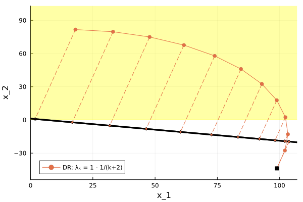
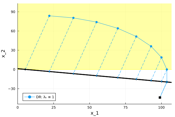
To further illustrate the behaviour of the considered numerical methods, we plot below some generated trajectories in case n:=1n:=1, and for u=(1,5)Tu=(1,5)^{T} and ν:=6\nu:=6. The generated sequences by the different methods may converge to different solutions for the same starting point which is plotted as a black square in the figures. However, the way the iterates of the DR algorithms and the Halpern algorithm, on the one hand, an the Fast KM algorithm, on the other hand, tend to their limits through are totally different. While the iterates of the DR algorithms and the Halpern algorithm move along a curve above the hyperplane Hu,νH_{u,\nu}, the ones generated by the Fast KM algorithm approach in a more straight manner the solution.

In the figures fig. 18 and fig. 18 we plot the trajectory generated by the Halpern algorithm for two different starting points in order to emphasize their pronounced spiralling around the limit point. This also explains why (see also fig. 14), even if the algorithm finds a solution in less than 𝚔max\mathtt{k_{\max}} steps, it requires more iterations than the DR algorithms and significantly more than the Fast KM algorithm.
Refer to caption
Figure 11: The trajectory of the Douglas-Rachford algorithm for sk:=1−1k+2s_{k}:=1-\frac{1}{k+2}
Refer to caption
Figure 12: The trajectory of the Douglas-Rachford algorithm for sk:=1s_{k}:=1
Refer to caption
Figure 13: The trajectory of the Douglas-Rachford algorithm for sk:=32s_{k}:=\frac{3}{2}
Refer to caption
Figure 14: The trajectory of the Halpern algorithm
Refer to caption
Figure 15: The trajectory of the Fast KM algorithm for α=5\alpha=5
Refer to caption
Figure 16: The trajectory of the Fast KM algorithm for α=30\alpha=30
Refer to caption
Figure 17: An instance for which the Halpern algorithm does not terminates in less than 𝚔max\mathtt{k_{\max}} iterations
Refer to caption
Figure 18: The spiral behavior of the Halpern algorithm

Appendix

In the appendix, we have compiled some auxiliary results and provided the proofs of the two technical lemmas used in the convergence analysis of the Fast KM algorithm.

Appendix A Auxiliary results

The Opial Lemma ([34]) is used in the proof of the convergence of the iterates.

Lemma 11.

Let 𝒮\mathcal{S} be a nonempty subset of ℋ\mathcal{H} and (xk)k≥0\left(x_{k}\right)_{k\geq 0} be a sequence in ℋ\mathcal{H}. Assume that

  1. (i)\rm{(i)}

    for every x∗∈𝒮x_{*}\in\mathcal{S}, limk→+∞‖xk−x∗‖\lim\limits_{k\to+\infty}\left\lVert x_{k}-x_{*}\right\rVert exists;

  2. (ii)\rm{(ii)}

    every weak sequential cluster point of the sequence (xk)k≥0\left(x_{k}\right)_{k\geq 0} as k→+∞k\to+\infty belongs to 𝒮\mathcal{S}.

Then (xk)k≥0\left(x_{k}\right)_{k\geq 0} converges weakly to a point in 𝒮\mathcal{S} as k→+∞k\to+\infty.

For the proof of the following result, which is the discrete counterpart of [1, Lemma A.2], we refer to [6, Lemma 21].

Lemma 12.

Let a≥1a\geq 1 and (qk)k≥0\left(q_{k}\right)_{k\geq 0} be a bounded sequence in ℋ\mathcal{H} such that

limk→+∞(qk+1+ka​(qk+1−qk))=l∈ℋ.\lim\limits_{k\to+\infty}\left(q_{k+1}+\dfrac{k}{a}\left(q_{k+1}-q_{k}\right)\right)=l\in\mathcal{H}.

Then it holds limk→+∞qk=l\lim\limits_{k\to+\infty}q_{k}=l.

The following result is a particular instance of [3, Lemma 5.31].

Lemma 13.

Let (ak)k≥1\left(a_{k}\right)_{k\geq 1}, (bk)k≥1\left(b_{k}\right)_{k\geq 1} and (dk)k≥1\left(d_{k}\right)_{k\geq 1} be sequences of real numbers. Assume that (ak)k≥1\left(a_{k}\right)_{k\geq 1} is bounded from below, and (bk)k≥1\left(b_{k}\right)_{k\geq 1} and (dk)k≥1\left(d_{k}\right)_{k\geq 1} are nonnegative sequences such that ∑k≥1dk<+∞\sum_{k\geq 1}d_{k}<+\infty. If

ak+1≤ak−bk+dk∀k≥1,a_{k+1}\leq a_{k}-b_{k}+d_{k}\quad\forall k\geq 1,

then the following statements are true:

  1. (i)\rm{(i)}

    the sequence (bk)k≥1\left(b_{k}\right)_{k\geq 1} is summable, namely ∑k≥1bk<+∞\sum_{k\geq 1}b_{k}<+\infty;

  2. (ii)\rm{(ii)}

    the sequence (ak)k≥1\left(a_{k}\right)_{k\geq 1} is convergent.

The following elementary result is used several times in the paper.

Lemma 14.

Let a,b,c∈ℝa,b,c\in\mathbb{R} be such that a<0a<0 and b2−a​c≤0b^{2}-ac\leq 0. Then it holds

a​‖x‖2+2​b​⟨x,y⟩+c​‖y‖2≤0∀x,y∈ℋ.a\left\lVert x\right\rVert^{2}+2b\left\langle x,y\right\rangle+c\left\lVert y\right\rVert^{2}\leq 0\quad\forall x,y\in\mathcal{H}.

Appendix B Proofs of the technical lemmas used in the analysis of the Fast KM algorithm

In this subsection we provide the proofs of lemma 3 and lemma 4.

Proof of lemma 3.

( i ) Let 0≤λ≤α−10\leq\lambda\leq\alpha-1. First we will show that for every k≥1k\geq 1 the following identity holds

(ℰλ,k+1+14​(α−1)​(α−2)​α​s2​(k+1)​‖(Id−T)​(xk)‖2)\displaystyle\left(\mathcal{E}_{\lambda,k+1}+\dfrac{1}{4\left(\alpha-1\right)}\left(\alpha-2\right)\alpha s^{2}\left(k+1\right)\left\lVert\left(\mathrm{Id}-T\right)\left(x_{k}\right)\right\rVert^{2}\right) (30)
−(ℰλ,k+14​(α−1)​(α−2)​α​s2​k​‖(Id−T)​(xk−1)‖2)\displaystyle\quad\ \ -\left(\mathcal{E}_{\lambda,k}+\dfrac{1}{4\left(\alpha-1\right)}\left(\alpha-2\right)\alpha s^{2}k\left\lVert\left(\mathrm{Id}-T\right)\left(x_{k-1}\right)\right\rVert^{2}\right)
=\displaystyle= 2​(2−α)​λ​s​⟨xk+1−x∗,(Id−T)​(xk)⟩+2​(λ+1−α)​(2​k+α+1)​‖xk+1−xk‖2\displaystyle\ 2\left(2-\alpha\right)\lambda s\left\langle x_{k+1}-x_{*},\left(\mathrm{Id}-T\right)\left(x_{k}\right)\right\rangle+2\left(\lambda+1-\alpha\right)\left(2k+\alpha+1\right)\left\lVert x_{k+1}-x_{k}\right\rVert^{2}
+14​(α−1)​(2−α)​s2​(2​(3​α−2)​k+2​α2+α−2)​‖(Id−T)​(xk)‖2\displaystyle+\dfrac{1}{4\left(\alpha-1\right)}\left(2-\alpha\right)s^{2}\left(2\left(3\alpha-2\right)k+2\alpha^{2}+\alpha-2\right)\left\lVert\left(\mathrm{Id}-T\right)\left(x_{k}\right)\right\rVert^{2}
+1α−1​(4​(α−1)​(λ+1−α)+α⁡(2−α))​s​k​⟨xk+1−xk,(Id−T)​(xk)⟩\displaystyle+\dfrac{1}{\alpha-1}\Bigl(4\left(\alpha-1\right)\left(\lambda+1-\alpha\right)+\alpha\left(2-\alpha\right)\Bigr)sk\left\langle x_{k+1}-x_{k},\left(\mathrm{Id}-T\right)\left(x_{k}\right)\right\rangle
+1α−1​(2​α​(α−1)​(λ+1−α)+α−2​(α−1)2)​s​⟨xk+1−xk,(Id−T)​(xk)⟩\displaystyle+\dfrac{1}{\alpha-1}\left(2\alpha\left(\alpha-1\right)\left(\lambda+1-\alpha\right)+\alpha-2\left(\alpha-1\right)^{2}\right)s\left\langle x_{k+1}-x_{k},\left(\mathrm{Id}-T\right)\left(x_{k}\right)\right\rangle
+1α−1​(2−α)​s​(k+α)​k​⟨xk+1−xk,(Id−T)​(xk)−(Id−T)​(xk−1)⟩\displaystyle+\dfrac{1}{\alpha-1}\left(2-\alpha\right)s\left(k+\alpha\right)k\left\langle x_{k+1}-x_{k},\left(\mathrm{Id}-T\right)\left(x_{k}\right)-\left(\mathrm{Id}-T\right)\left(x_{k-1}\right)\right\rangle
+14​(α−1)​(2−α)​s2​k​(2​k+α)​‖(Id−T)​(xk)−(Id−T)​(xk−1)‖2.\displaystyle+\dfrac{1}{4\left(\alpha-1\right)}\left(2-\alpha\right)s^{2}k\bigl(2k+\alpha\bigr)\left\lVert\left(\mathrm{Id}-T\right)\left(x_{k}\right)-\left(\mathrm{Id}-T\right)\left(x_{k-1}\right)\right\rVert^{2}.

For brevity we denote for every k≥0k\geq 0

uλ,k+1\displaystyle u_{\lambda,k+1} :=2​λ​(xk+1−x∗)+2​(k+1)​(xk+1−xk)\displaystyle:=2\lambda\left(x_{k+1}-x_{*}\right)+2\left(k+1\right)\left(x_{k+1}-x_{k}\right) (31)
+12​(α−1)​(3​α−2)​s​(k+1)​(Id−T)​(xk),\displaystyle\qquad+\dfrac{1}{2\left(\alpha-1\right)}\left(3\alpha-2\right)s\left(k+1\right)\left(\mathrm{Id}-T\right)\left(x_{k}\right),

which means that for every k≥1k\geq 1 it holds

uλ,k=2​λ​(xk−x∗)+2​k​(xk−xk−1)+12​(α−1)​(3​α−2)​s​k​(Id−T)​(xk−1).u_{\lambda,k}=2\lambda\left(x_{k}-x_{*}\right)+2k\left(x_{k}-x_{k-1}\right)+\dfrac{1}{2\left(\alpha-1\right)}\left(3\alpha-2\right)sk\left(\mathrm{Id}-T\right)\left(x_{k-1}\right). (32)

Subtracting (32) from (31) and then using (10) we obtain for every k≥1k\geq 1

uλ,k+1−uλ,k\displaystyle\ u_{\lambda,k+1}-u_{\lambda,k} (33)
=\displaystyle= 2​(λ+1−α)​(xk+1−xk)+2​(k+α)​(xk+1−xk)−2​k​(xk−xk−1)\displaystyle\ 2\left(\lambda+1-\alpha\right)\left(x_{k+1}-x_{k}\right)+2\left(k+\alpha\right)\left(x_{k+1}-x_{k}\right)-2k\left(x_{k}-x_{k-1}\right)
+12​(α−1)​(3​α−2)​s​(Id−T)​(xk)\displaystyle+\dfrac{1}{2\left(\alpha-1\right)}\left(3\alpha-2\right)s\left(\mathrm{Id}-T\right)\left(x_{k}\right)
+12​(α−1)​(3​α−2)​s​k​((Id−T)​(xk)−(Id−T)​(xk−1))\displaystyle+\dfrac{1}{2\left(\alpha-1\right)}\left(3\alpha-2\right)sk\Bigl(\left(\mathrm{Id}-T\right)\left(x_{k}\right)-\left(\mathrm{Id}-T\right)\left(x_{k-1}\right)\Bigr)
=\displaystyle= 2​(λ+1−α)​(xk+1−xk)+12​(α−1)​(α−2​(α−1)2)​s​(Id−T)​(xk)\displaystyle\ 2\left(\lambda+1-\alpha\right)\left(x_{k+1}-x_{k}\right)+\dfrac{1}{2\left(\alpha-1\right)}\left(\alpha-2\left(\alpha-1\right)^{2}\right)s\left(\mathrm{Id}-T\right)\left(x_{k}\right)
+12​(α−1)​(2−α)​s​k​((Id−T)​(xk)−(Id−T)​(xk−1)).\displaystyle+\dfrac{1}{2\left(\alpha-1\right)}\left(2-\alpha\right)sk\Bigl(\left(\mathrm{Id}-T\right)\left(x_{k}\right)-\left(\mathrm{Id}-T\right)\left(x_{k-1}\right)\Bigr).

In the following we want to use the identity

12​(‖uλ,k+1‖2−‖uλ,k‖2)=⟨uλ,k+1,uλ,k+1−uλ,k⟩−12​‖uλ,k+1−uλ,k‖2∀k≥1.\dfrac{1}{2}\left(\left\lVert u_{\lambda,k+1}\right\rVert^{2}-\left\lVert u_{\lambda,k}\right\rVert^{2}\right)=\left\langle u_{\lambda,k+1},u_{\lambda,k+1}-u_{\lambda,k}\right\rangle-\dfrac{1}{2}\left\lVert u_{\lambda,k+1}-u_{\lambda,k}\right\rVert^{2}\quad\forall k\geq 1. (34)

Thanks to the relations (31) and (33), we derive for every k≥1k\geq 1 that

⟨uλ,k+1,uλ,k+1−uλ,k⟩\displaystyle\left\langle u_{\lambda,k+1},u_{\lambda,k+1}-u_{\lambda,k}\right\rangle (35)
=\displaystyle= 4​λ​(λ+1−α)​⟨xk+1−x∗,xk+1−xk⟩\displaystyle\ 4\lambda\left(\lambda+1-\alpha\right)\left\langle x_{k+1}-x_{*},x_{k+1}-x_{k}\right\rangle
+1α−1​(α−2​(α−1)2)​λ​s​⟨xk+1−x∗,(Id−T)​(xk)⟩\displaystyle+\dfrac{1}{\alpha-1}\left(\alpha-2\left(\alpha-1\right)^{2}\right)\lambda s\left\langle x_{k+1}-x_{*},\left(\mathrm{Id}-T\right)\left(x_{k}\right)\right\rangle
+1α−1​(2−α)​λ​s​k​⟨xk+1−x∗,(Id−T)​(xk)−(Id−T)​(xk−1)⟩\displaystyle+\dfrac{1}{\alpha-1}\left(2-\alpha\right)\lambda sk\left\langle x_{k+1}-x_{*},\left(\mathrm{Id}-T\right)\left(x_{k}\right)-\left(\mathrm{Id}-T\right)\left(x_{k-1}\right)\right\rangle
+4​(λ+1−α)​(k+1)​‖xk+1−xk‖2\displaystyle+4\left(\lambda+1-\alpha\right)\left(k+1\right)\left\lVert x_{k+1}-x_{k}\right\rVert^{2}
+1α−1​(α−2​(α−1)2+(3​α−2)​(λ+1−α))​s​(k+1)​⟨xk+1−xk,(Id−T)​(xk)⟩\displaystyle+\dfrac{1}{\alpha-1}\Bigl(\alpha-2\left(\alpha-1\right)^{2}+\left(3\alpha-2\right)\left(\lambda+1-\alpha\right)\Bigr)s\left(k+1\right)\left\langle x_{k+1}-x_{k},\left(\mathrm{Id}-T\right)\left(x_{k}\right)\right\rangle
+1α−1​(2−α)​s​(k+1)​k​⟨xk+1−xk,(Id−T)​(xk)−(Id−T)​(xk−1)⟩\displaystyle+\dfrac{1}{\alpha-1}\left(2-\alpha\right)s\left(k+1\right)k\left\langle x_{k+1}-x_{k},\left(\mathrm{Id}-T\right)\left(x_{k}\right)-\left(\mathrm{Id}-T\right)\left(x_{k-1}\right)\right\rangle
+14​(α−1)2​(3​α−2)​(α−2​(α−1)2)​s2​(k+1)​‖(Id−T)​(xk)‖2\displaystyle+\dfrac{1}{4\left(\alpha-1\right)^{2}}\left(3\alpha-2\right)\left(\alpha-2\left(\alpha-1\right)^{2}\right)s^{2}\left(k+1\right)\left\lVert\left(\mathrm{Id}-T\right)\left(x_{k}\right)\right\rVert^{2}
+14​(α−1)2(3α−2)(2−α)s2(k+1)k⟨(Id−T)(xk),\displaystyle+\dfrac{1}{4\left(\alpha-1\right)^{2}}\left(3\alpha-2\right)\left(2-\alpha\right)s^{2}\left(k+1\right)k\left\langle\left(\mathrm{Id}-T\right)\left(x_{k}\right),\right.
(Id−T)(xk)−(Id−T)(xk−1)⟩,\displaystyle\hskip 213.39566pt\left.\left(\mathrm{Id}-T\right)\left(x_{k}\right)-\left(\mathrm{Id}-T\right)\left(x_{k-1}\right)\right\rangle,

and

−12​‖uλ,k+1−uλ,k‖2\displaystyle-\dfrac{1}{2}\left\lVert u_{\lambda,k+1}-u_{\lambda,k}\right\rVert^{2} (36)
=\displaystyle= −2​(λ+1−α)2​‖xk+1−xk‖2−18​(α−1)2​(α−2​(α−1)2)2​s2​‖(Id−T)​(xk)‖2\displaystyle-2\left(\lambda+1-\alpha\right)^{2}\left\lVert x_{k+1}-x_{k}\right\rVert^{2}-\dfrac{1}{8\left(\alpha-1\right)^{2}}\left(\alpha-2\left(\alpha-1\right)^{2}\right)^{2}s^{2}\left\lVert\left(\mathrm{Id}-T\right)\left(x_{k}\right)\right\rVert^{2}
−18​(α−1)2​(2−α)2​s2​k2​‖(Id−T)​(xk)−(Id−T)​(xk−1)‖2\displaystyle-\dfrac{1}{8\left(\alpha-1\right)^{2}}\left(2-\alpha\right)^{2}s^{2}k^{2}\left\lVert\left(\mathrm{Id}-T\right)\left(x_{k}\right)-\left(\mathrm{Id}-T\right)\left(x_{k-1}\right)\right\rVert^{2}
−1α−1​(α−2​(α−1)2)​(λ+1−α)​s​⟨xk+1−xk,(Id−T)​(xk)⟩\displaystyle-\dfrac{1}{\alpha-1}\left(\alpha-2\left(\alpha-1\right)^{2}\right)\left(\lambda+1-\alpha\right)s\left\langle x_{k+1}-x_{k},\left(\mathrm{Id}-T\right)\left(x_{k}\right)\right\rangle
−1α−1​(2−α)​(λ+1−α)​s​k​⟨xk+1−xk,(Id−T)​(xk)−(Id−T)​(xk−1)⟩\displaystyle-\dfrac{1}{\alpha-1}\left(2-\alpha\right)\left(\lambda+1-\alpha\right)sk\left\langle x_{k+1}-x_{k},\left(\mathrm{Id}-T\right)\left(x_{k}\right)-\left(\mathrm{Id}-T\right)\left(x_{k-1}\right)\right\rangle
−14​(α−1)2(α−2(α−1)2)(2−α)s2k⟨(Id−T)(xk),\displaystyle-\dfrac{1}{4\left(\alpha-1\right)^{2}}\left(\alpha-2\left(\alpha-1\right)^{2}\right)\left(2-\alpha\right)s^{2}k\left\langle\left(\mathrm{Id}-T\right)\left(x_{k}\right),\right.
(Id−T)(xk)−(Id−T)(xk−1)⟩.\displaystyle\hskip 170.71652pt\left.\left(\mathrm{Id}-T\right)\left(x_{k}\right)-\left(\mathrm{Id}-T\right)\left(x_{k-1}\right)\right\rangle.

A direct computation shows that for every k≥0k\geq 0

((3​α−2)​(λ+1−α)+α−2​(α−1)2)​(k+1)−(λ+1−α)​(α−2​(α−1)2)\displaystyle\left(\left(3\alpha-2\right)\left(\lambda+1-\alpha\right)+\alpha-2\left(\alpha-1\right)^{2}\right)\left(k+1\right)-\left(\lambda+1-\alpha\right)\left(\alpha-2\left(\alpha-1\right)^{2}\right)
=\displaystyle= ((3​α−2)​(λ+1−α)+α−2​(α−1)2)​k+2​α​(α−1)​(λ+1−α)+α−2​(α−1)2\displaystyle\left(\left(3\alpha-2\right)\left(\lambda+1-\alpha\right)+\alpha-2\left(\alpha-1\right)^{2}\right)k+2\alpha\left(\alpha-1\right)\left(\lambda+1-\alpha\right)+\alpha-2\left(\alpha-1\right)^{2}
=\displaystyle= ((3​α−2)​(λ+1−α)+α−2​(α−1)2−(2−α)​λ)​k+(2−α)​λ​k\displaystyle\left(\left(3\alpha-2\right)\left(\lambda+1-\alpha\right)+\alpha-2\left(\alpha-1\right)^{2}-\left(2-\alpha\right)\lambda\right)k+\left(2-\alpha\right)\lambda k
+2​α​(α−1)​(λ+1−α)+α−2​(α−1)2\displaystyle+2\alpha\left(\alpha-1\right)\left(\lambda+1-\alpha\right)+\alpha-2\left(\alpha-1\right)^{2}
=\displaystyle= (4​(α−1)​(λ+1−α)+α⁡(2−α))​k+(2−α)​λ​k\displaystyle\Bigl(4\left(\alpha-1\right)\left(\lambda+1-\alpha\right)+\alpha\left(2-\alpha\right)\Bigr)k+\left(2-\alpha\right)\lambda k
+2​α​(α−1)​(λ+1−α)+α−2​(α−1)2.\displaystyle+2\alpha\left(\alpha-1\right)\left(\lambda+1-\alpha\right)+\alpha-2\left(\alpha-1\right)^{2}.

Therefore, by plugging (35) and (36) into (34), we get for every k≥1k\geq 1

12​(‖uλ,k+1‖2−‖uλ,k‖2)\displaystyle\quad\dfrac{1}{2}\left(\left\lVert u_{\lambda,k+1}\right\rVert^{2}-\left\lVert u_{\lambda,k}\right\rVert^{2}\right) (37)
= 4​λ​(λ+1−α)​⟨xk+1−x∗,xk+1−xk⟩\displaystyle=\ 4\lambda\left(\lambda+1-\alpha\right)\left\langle x_{k+1}-x_{*},x_{k+1}-x_{k}\right\rangle
+1α−1​(α−2​(α−1)2)​λ​s​⟨xk+1−x∗,(Id−T)​(xk)⟩\displaystyle+\dfrac{1}{\alpha-1}\left(\alpha-2\left(\alpha-1\right)^{2}\right)\lambda s\left\langle x_{k+1}-x_{*},\left(\mathrm{Id}-T\right)\left(x_{k}\right)\right\rangle
+1α−1​(2−α)​λ​s​k​⟨xk+1−x∗,(Id−T)​(xk)−(Id−T)​(xk−1)⟩\displaystyle+\dfrac{1}{\alpha-1}\left(2-\alpha\right)\lambda sk\left\langle x_{k+1}-x_{*},\left(\mathrm{Id}-T\right)\left(x_{k}\right)-\left(\mathrm{Id}-T\right)\left(x_{k-1}\right)\right\rangle
+2​(λ+1−α)​(2​k+α+1−λ)​‖xk+1−xk‖2\displaystyle+2\left(\lambda+1-\alpha\right)\left(2k+\alpha+1-\lambda\right)\left\lVert x_{k+1}-x_{k}\right\rVert^{2}
+18​(α−1)2​(α−2​(α−1)2)​s2​(2​(3​α−2)​k+2​α2+α−2)​‖(Id−T)​(xk)‖2\displaystyle+\dfrac{1}{8\left(\alpha-1\right)^{2}}\left(\alpha-2\left(\alpha-1\right)^{2}\right)s^{2}\left(2\left(3\alpha-2\right)k+2\alpha^{2}+\alpha-2\right)\left\lVert\left(\mathrm{Id}-T\right)\left(x_{k}\right)\right\rVert^{2}
+1α−1​(4​(α−1)​(λ+1−α)+α⁡(2−α)+(2−α)​λ)​s​k​⟨xk+1−xk,(Id−T)​(xk)⟩\displaystyle+\dfrac{1}{\alpha-1}\Bigl(4\left(\alpha-1\right)\left(\lambda+1-\alpha\right)+\alpha\left(2-\alpha\right)+\left(2-\alpha\right)\lambda\Bigr)sk\left\langle x_{k+1}-x_{k},\left(\mathrm{Id}-T\right)\left(x_{k}\right)\right\rangle
+1α−1​(2​α​(α−1)​(λ+1−α)+α−2​(α−1)2)​s​⟨xk+1−xk,(Id−T)​(xk)⟩\displaystyle+\dfrac{1}{\alpha-1}\left(2\alpha\left(\alpha-1\right)\left(\lambda+1-\alpha\right)+\alpha-2\left(\alpha-1\right)^{2}\right)s\left\langle x_{k+1}-x_{k},\left(\mathrm{Id}-T\right)\left(x_{k}\right)\right\rangle
+1α−1​(2−α)​s​(k+α−λ)​k​⟨xk+1−xk,(Id−T)​(xk)−(Id−T)​(xk−1)⟩\displaystyle+\dfrac{1}{\alpha-1}\left(2-\alpha\right)s\left(k+\alpha-\lambda\right)k\left\langle x_{k+1}-x_{k},\left(\mathrm{Id}-T\right)\left(x_{k}\right)-\left(\mathrm{Id}-T\right)\left(x_{k-1}\right)\right\rangle
+14​(α−1)2(2−α)s2((3α−2)k+2(α−1)α)k⟨(Id−T)(xk),\displaystyle+\dfrac{1}{4\left(\alpha-1\right)^{2}}\left(2-\alpha\right)s^{2}\left(\left(3\alpha-2\right)k+2\left(\alpha-1\right)\alpha\right)k\left\langle\left(\mathrm{Id}-T\right)\left(x_{k}\right),\right.
(Id−T)(xk)−(Id−T)(xk−1)⟩\displaystyle\hskip 170.71652pt\left.\left(\mathrm{Id}-T\right)\left(x_{k}\right)-\left(\mathrm{Id}-T\right)\left(x_{k-1}\right)\right\rangle
−18​(α−1)2​(2−α)2​s2​k2​‖(Id−T)​(xk)−(Id−T)​(xk−1)‖2.\displaystyle-\dfrac{1}{8\left(\alpha-1\right)^{2}}\left(2-\alpha\right)^{2}s^{2}k^{2}\left\lVert\left(\mathrm{Id}-T\right)\left(x_{k}\right)-\left(\mathrm{Id}-T\right)\left(x_{k-1}\right)\right\rVert^{2}.

Notice that by the definition of the energy function we have for every k≥1k\geq 1

ℰλ,k+14​(α−1)​(α−2)​α​s2​k​‖(Id−T)​(xk−1)‖2\displaystyle\ \mathcal{E}_{\lambda,k}+\dfrac{1}{4\left(\alpha-1\right)}\left(\alpha-2\right)\alpha s^{2}k\left\lVert\left(\mathrm{Id}-T\right)\left(x_{k-1}\right)\right\rVert^{2} (38)
=\displaystyle= 12​‖uλ,k‖2+2​λ​(α−1−λ)​‖xk−x∗‖2\displaystyle\ \dfrac{1}{2}\left\lVert u_{\lambda,k}\right\rVert^{2}+2\lambda\left(\alpha-1-\lambda\right)\left\lVert x_{k}-x_{*}\right\rVert^{2}
+1α−1​(α−2)​λ​s​k​⟨xk−x∗,(Id−T)​(xk−1)⟩\displaystyle+\dfrac{1}{\alpha-1}\left(\alpha-2\right)\lambda sk\left\langle x_{k}-x_{*},\left(\mathrm{Id}-T\right)\left(x_{k-1}\right)\right\rangle
+18​(α−1)2​(α−2)​s2​k​((3​α−2)​k+2​(α−1)​α)​‖(Id−T)​(xk−1)‖2.\displaystyle+\dfrac{1}{8\left(\alpha-1\right)^{2}}(\alpha-2)s^{2}k\left(\left(3\alpha-2\right)k+2(\alpha-1)\alpha\right)\left\lVert\left(\mathrm{Id}-T\right)\left(x_{k-1}\right)\right\rVert^{2}.

Later we will subtract the above identity at consecutive indices and to this end we will make use of the following identities which hold for every k≥1k\geq 1:

‖xk+1−x∗‖2−‖xk−x∗‖2=2​⟨xk+1−x∗,xk+1−xk⟩−‖xk+1−xk‖2,\displaystyle\left\lVert x_{k+1}-x_{*}\right\rVert^{2}-\left\lVert x_{k}-x_{*}\right\rVert^{2}=2\left\langle x_{k+1}-x_{*},x_{k+1}-x_{k}\right\rangle-\left\lVert x_{k+1}-x_{k}\right\rVert^{2}, (39)
2​λ​s​(k+1)​⟨xk+1−x∗,(Id−T)​(xk)⟩−2​λ​s​k​⟨xk−x∗,(Id−T)​(xk−1)⟩\displaystyle\ 2\lambda s\left(k+1\right)\left\langle x_{k+1}-x_{*},\left(\mathrm{Id}-T\right)\left(x_{k}\right)\right\rangle-2\lambda sk\left\langle x_{k}-x_{*},\left(\mathrm{Id}-T\right)\left(x_{k-1}\right)\right\rangle (40)
=\displaystyle= 2​λ​s​k​(⟨xk+1−x∗,(Id−T)​(xk)⟩−⟨xk−x∗,(Id−T)​(xk−1)⟩)\displaystyle\ 2\lambda sk\Bigl(\left\langle x_{k+1}-x_{*},\left(\mathrm{Id}-T\right)\left(x_{k}\right)\right\rangle-\left\langle x_{k}-x_{*},\left(\mathrm{Id}-T\right)\left(x_{k-1}\right)\right\rangle\Bigr)
+2​λ​s​⟨xk+1−x∗,(Id−T)​(xk)⟩\displaystyle+2\lambda s\left\langle x_{k+1}-x_{*},\left(\mathrm{Id}-T\right)\left(x_{k}\right)\right\rangle
=\displaystyle= 2​λ​s​k​⟨xk+1−x∗,(Id−T)​(xk)−(Id−T)​(xk−1)⟩\displaystyle\ 2\lambda sk\left\langle x_{k+1}-x_{*},\left(\mathrm{Id}-T\right)\left(x_{k}\right)-\left(\mathrm{Id}-T\right)\left(x_{k-1}\right)\right\rangle
+2​λ​s​k​⟨xk+1−xk,(Id−T)​(xk−1)⟩+2​λ​s​⟨xk+1−x∗,(Id−T)​(xk)⟩\displaystyle+2\lambda sk\left\langle x_{k+1}-x_{k},\left(\mathrm{Id}-T\right)\left(x_{k-1}\right)\right\rangle+2\lambda s\left\langle x_{k+1}-x_{*},\left(\mathrm{Id}-T\right)\left(x_{k}\right)\right\rangle
=\displaystyle= 2​λ​s​k​⟨xk+1−x∗,(Id−T)​(xk)−(Id−T)​(xk−1)⟩\displaystyle\ 2\lambda sk\left\langle x_{k+1}-x_{*},\left(\mathrm{Id}-T\right)\left(x_{k}\right)-\left(\mathrm{Id}-T\right)\left(x_{k-1}\right)\right\rangle
−2​λ​s​k​⟨xk+1−xk,(Id−T)​(xk)−(Id−T)​(xk−1)⟩\displaystyle-2\lambda sk\left\langle x_{k+1}-x_{k},\left(\mathrm{Id}-T\right)\left(x_{k}\right)-\left(\mathrm{Id}-T\right)\left(x_{k-1}\right)\right\rangle
+2​λ​s​k​⟨xk+1−xk,(Id−T)​(xk)⟩+2​λ​s​⟨xk+1−x∗,(Id−T)​(xk)⟩,\displaystyle+2\lambda sk\left\langle x_{k+1}-x_{k},\left(\mathrm{Id}-T\right)\left(x_{k}\right)\right\rangle+2\lambda s\left\langle x_{k+1}-x_{*},\left(\mathrm{Id}-T\right)\left(x_{k}\right)\right\rangle,

and

14​(α−1)​s2​(k+1)​((3​α−2)​(k+1)+2​(α−1)​α)​‖(Id−T)​(xk)‖2\displaystyle\ \dfrac{1}{4\left(\alpha-1\right)}s^{2}\left(k+1\right)\bigl(\left(3\alpha-2\right)\left(k+1\right)+2\left(\alpha-1\right)\alpha\bigr)\left\lVert\left(\mathrm{Id}-T\right)\left(x_{k}\right)\right\rVert^{2} (41)
−14​(α−1)​s2​k​((3​α−2)​k+2​(α−1)​α)​‖(Id−T)​(xk−1)‖2\displaystyle\ -\dfrac{1}{4\left(\alpha-1\right)}s^{2}k\bigl(\left(3\alpha-2\right)k+2\left(\alpha-1\right)\alpha\bigr)\left\lVert\left(\mathrm{Id}-T\right)\left(x_{k-1}\right)\right\rVert^{2}
=\displaystyle= 14​(α−1)​s2​(2​(3​α−2)​k+2​α2+α−2)​‖(Id−T)​(xk)‖2\displaystyle\ \dfrac{1}{4\left(\alpha-1\right)}s^{2}\bigl(2\left(3\alpha-2\right)k+2\alpha^{2}+\alpha-2\bigr)\left\lVert\left(\mathrm{Id}-T\right)\left(x_{k}\right)\right\rVert^{2}
+14​(α−1)​s2​k​((3​α−2)​k+2​(α−1)​α)​(‖(Id−T)​(xk)‖2−‖(Id−T)​(xk−1)‖2)\displaystyle\ +\dfrac{1}{4\left(\alpha-1\right)}s^{2}k\left(\left(3\alpha-2\right)k+2\left(\alpha-1\right)\alpha\right)\left(\left\lVert\left(\mathrm{Id}-T\right)\left(x_{k}\right)\right\rVert^{2}-\left\lVert\left(\mathrm{Id}-T\right)\left(x_{k-1}\right)\right\rVert^{2}\right)
=\displaystyle= 14​(α−1)​s2​(2​(3​α−2)​k+2​α2+α−2)​‖(Id−T)​(xk)‖2\displaystyle\ \dfrac{1}{4\left(\alpha-1\right)}s^{2}\bigl(2\left(3\alpha-2\right)k+2\alpha^{2}+\alpha-2\bigr)\left\lVert\left(\mathrm{Id}-T\right)\left(x_{k}\right)\right\rVert^{2}
+12​(α−1)s2k((3α−2)k+2(α−1)α)⟨(Id−T)(xk),\displaystyle\ +\dfrac{1}{2\left(\alpha-1\right)}s^{2}k\bigl(\left(3\alpha-2\right)k+2\left(\alpha-1\right)\alpha\bigr)\left\langle\left(\mathrm{Id}-T\right)\left(x_{k}\right),\right.
(Id−T)(xk)−(Id−T)(xk−1)⟩\displaystyle\hskip 199.16928pt\left.\left(\mathrm{Id}-T\right)\left(x_{k}\right)-\left(\mathrm{Id}-T\right)\left(x_{k-1}\right)\right\rangle
−14​(α−1)​s2​k​((3​α−2)​k+2​(α−1)​α)​‖(Id−T)​(xk)−(Id−T)​(xk−1)‖2.\displaystyle\ -\dfrac{1}{4\left(\alpha-1\right)}s^{2}k\bigl(\left(3\alpha-2\right)k+2\left(\alpha-1\right)\alpha\bigr)\left\lVert\left(\mathrm{Id}-T\right)\left(x_{k}\right)-\left(\mathrm{Id}-T\right)\left(x_{k-1}\right)\right\rVert^{2}.

Therefore, by multiplying (40) and (41) by 12​(α−1)​(α−2)\frac{1}{2\left(\alpha-1\right)}\left(\alpha-2\right), relation (38) gives for every k≥1k\geq 1

(ℰλ,k+1+14​(α−1)​(α−2)​α​s2​(k+1)​‖(Id−T)​(xk)‖2)\displaystyle\left(\mathcal{E}_{\lambda,k+1}+\dfrac{1}{4\left(\alpha-1\right)}\left(\alpha-2\right)\alpha s^{2}\left(k+1\right)\left\lVert\left(\mathrm{Id}-T\right)\left(x_{k}\right)\right\rVert^{2}\right)
−(ℰλ,k+14​(α−1)​(α−2)​α​s2​k​‖(Id−T)​(xk−1)‖2)\displaystyle\quad\ \ -\left(\mathcal{E}_{\lambda,k}+\dfrac{1}{4\left(\alpha-1\right)}\left(\alpha-2\right)\alpha s^{2}k\left\lVert\left(\mathrm{Id}-T\right)\left(x_{k-1}\right)\right\rVert^{2}\right)
=12​(‖uλ,k+1‖2−‖uλ,k‖2)+2​λ​(α−1−λ)​(‖xk+1−x∗‖2−‖xk−x∗‖2)\displaystyle=\ \dfrac{1}{2}\left(\left\lVert u_{\lambda,k+1}\right\rVert^{2}-\left\lVert u_{\lambda,k}\right\rVert^{2}\right)+2\lambda(\alpha-1-\lambda)\left(\left\lVert x_{k+1}-x_{*}\right\rVert^{2}-\left\lVert x_{k}-x_{*}\right\rVert^{2}\right)
+1α−1​(α−2)​λ​s​⟨xk+1−x∗,(Id−T)​(xk)⟩\displaystyle+\dfrac{1}{\alpha-1}\left(\alpha-2\right)\lambda s\left\langle x_{k+1}-x_{*},\left(\mathrm{Id}-T\right)\left(x_{k}\right)\right\rangle
+1α−1​(α−2)​λ​s​k​⟨xk+1−x∗,(Id−T)​(xk)−(Id−T)​(xk−1)⟩\displaystyle+\dfrac{1}{\alpha-1}\left(\alpha-2\right)\lambda sk\left\langle x_{k+1}-x_{*},\left(\mathrm{Id}-T\right)\left(x_{k}\right)-\left(\mathrm{Id}-T\right)\left(x_{k-1}\right)\right\rangle
−1α−1​(α−2)​λ​s​k​⟨xk+1−xk,(Id−T)​(xk)−(Id−T)​(xk−1)⟩\displaystyle-\dfrac{1}{\alpha-1}\left(\alpha-2\right)\lambda sk\left\langle x_{k+1}-x_{k},\left(\mathrm{Id}-T\right)\left(x_{k}\right)-\left(\mathrm{Id}-T\right)\left(x_{k-1}\right)\right\rangle
+1α−1​(α−2)​λ​s​k​⟨xk+1−xk,(Id−T)​(xk)⟩\displaystyle+\dfrac{1}{\alpha-1}\left(\alpha-2\right)\lambda sk\left\langle x_{k+1}-x_{k},\left(\mathrm{Id}-T\right)\left(x_{k}\right)\right\rangle
+18​(α−1)2​(α−2)​s2​(2​(3​α−2)​k+2​α2+α−2)​‖(Id−T)​(xk)‖2\displaystyle+\dfrac{1}{8\left(\alpha-1\right)^{2}}\left(\alpha-2\right)s^{2}\bigl(2\left(3\alpha-2\right)k+2\alpha^{2}+\alpha-2\bigr)\left\lVert\left(\mathrm{Id}-T\right)\left(x_{k}\right)\right\rVert^{2}
+14​(α−1)2(α−2)s2k((3α−2)k+2(α−1)α)⟨(Id−T)(xk),\displaystyle+\dfrac{1}{4\left(\alpha-1\right)^{2}}\left(\alpha-2\right)s^{2}k\bigl(\left(3\alpha-2\right)k+2\left(\alpha-1\right)\alpha\bigr)\left\langle\left(\mathrm{Id}-T\right)\left(x_{k}\right),\right.
(Id−T)(xk)−(Id−T)(xk−1)⟩\displaystyle\hskip 199.16928pt\left.\left(\mathrm{Id}-T\right)\left(x_{k}\right)-\left(\mathrm{Id}-T\right)\left(x_{k-1}\right)\right\rangle
−18​(α−1)2​(α−2)​s2​k​((3​α−2)​k+2​(α−1)​α)​‖(Id−T)​(xk)−(Id−T)​(xk−1)‖2\displaystyle-\dfrac{1}{8\left(\alpha-1\right)^{2}}\left(\alpha-2\right)s^{2}k\bigl(\left(3\alpha-2\right)k+2\left(\alpha-1\right)\alpha\bigr)\left\lVert\left(\mathrm{Id}-T\right)\left(x_{k}\right)-\left(\mathrm{Id}-T\right)\left(x_{k-1}\right)\right\rVert^{2}

By multiplying (39) by 2​λ​(α−1−λ)2\lambda(\alpha-1-\lambda) and by taking into consideration (37) and that

α−2​(α−1)2+α−2\displaystyle\alpha-2\left(\alpha-1\right)^{2}+\alpha-2 =2​(α−1)​(2−α)\displaystyle=2\left(\alpha-1\right)\left(2-\alpha\right)
−(α−2)2−(α−2)​(3​α−2)\displaystyle-\left(\alpha-2\right)^{2}-\left(\alpha-2\right)\left(3\alpha-2\right) =−4​(α−2)​(α−1),\displaystyle=-4\left(\alpha-2\right)\left(\alpha-1\right),

we immediately obtain from here identity (30).

Next we will focus on the term ⟨xk+1−xk,(Id−T)​(xk)−(Id−T)​(xk−1)⟩\left\langle x_{k+1}-x_{k},\left(\mathrm{Id}-T\right)\left(x_{k}\right)-\left(\mathrm{Id}-T\right)\left(x_{k-1}\right)\right\rangle for which we will provide an upper bound by exploiting the cocoercivity of Id−T\mathrm{Id}-T. Precisely, the relations (5) and (10) guarantee that for every k≥1k\geq 1

−2​s​k​(k+α)​⟨xk+1−xk,(Id−T)​(xk)−(Id−T)​(xk−1)⟩\displaystyle-2sk\left(k+\alpha\right)\left\langle x_{k+1}-x_{k},\left(\mathrm{Id}-T\right)\left(x_{k}\right)-\left(\mathrm{Id}-T\right)\left(x_{k-1}\right)\right\rangle
=\displaystyle= −2​s​k2​⟨xk−xk−1,(Id−T)​(xk)−(Id−T)​(xk−1)⟩\displaystyle-2sk^{2}\left\langle x_{k}-x_{k-1},\left(\mathrm{Id}-T\right)\left(x_{k}\right)-\left(\mathrm{Id}-T\right)\left(x_{k-1}\right)\right\rangle
+2​s2​k2​‖(Id−T)​(xk)−(Id−T)​(xk−1)‖2\displaystyle+2s^{2}k^{2}\left\lVert\left(\mathrm{Id}-T\right)\left(x_{k}\right)-\left(\mathrm{Id}-T\right)\left(x_{k-1}\right)\right\rVert^{2}
+α​s2​k​⟨(Id−T)​(xk),(Id−T)​(xk)−(Id−T)​(xk−1)⟩\displaystyle+\alpha s^{2}k\left\langle\left(\mathrm{Id}-T\right)\left(x_{k}\right),\left(\mathrm{Id}-T\right)\left(x_{k}\right)-\left(\mathrm{Id}-T\right)\left(x_{k-1}\right)\right\rangle
≤\displaystyle\leq (2​s−1θ)​s​k2​‖(Id−T)​(xk)−(Id−T)​(xk−1)‖2+12​α​s2​k​‖(Id−T)​(xk)‖2\displaystyle\left(2s-\dfrac{1}{\theta}\right)sk^{2}\left\lVert\left(\mathrm{Id}-T\right)\left(x_{k}\right)-\left(\mathrm{Id}-T\right)\left(x_{k-1}\right)\right\rVert^{2}+\dfrac{1}{2}\alpha s^{2}k\left\lVert\left(\mathrm{Id}-T\right)\left(x_{k}\right)\right\rVert^{2}
+12​α​s2​k​‖(Id−T)​(xk)−(Id−T)​(xk−1)‖2−12​α​s2​k​‖(Id−T)​(xk−1)‖2\displaystyle+\dfrac{1}{2}\alpha s^{2}k\left\lVert\left(\mathrm{Id}-T\right)\left(x_{k}\right)-\left(\mathrm{Id}-T\right)\left(x_{k-1}\right)\right\rVert^{2}-\dfrac{1}{2}\alpha s^{2}k\left\lVert\left(\mathrm{Id}-T\right)\left(x_{k-1}\right)\right\rVert^{2}
≤\displaystyle\leq ((2​s−1θ)​s​k2+12​α​s2​k)​‖(Id−T)​(xk)−(Id−T)​(xk−1)‖2\displaystyle\left(\left(2s-\dfrac{1}{\theta}\right)sk^{2}+\dfrac{1}{2}\alpha s^{2}k\right)\left\lVert\left(\mathrm{Id}-T\right)\left(x_{k}\right)-\left(\mathrm{Id}-T\right)\left(x_{k-1}\right)\right\rVert^{2}
+12​α​s2​(k+1)​‖(Id−T)​(xk)‖2−12​α​s2​k​‖(Id−T)​(xk−1)‖2.\displaystyle+\dfrac{1}{2}\alpha s^{2}\left(k+1\right)\left\lVert\left(\mathrm{Id}-T\right)\left(x_{k}\right)\right\rVert^{2}-\dfrac{1}{2}\alpha s^{2}k\left\lVert\left(\mathrm{Id}-T\right)\left(x_{k-1}\right)\right\rVert^{2}.

After multiplying this inequality by 12​(α−1)​(α−2)>0\frac{1}{2\left(\alpha-1\right)}\left(\alpha-2\right)>0, adding it to(30), and using that

2​(2−α)​λ​s​⟨xk+1−x∗,(Id−T)​(xk)⟩\displaystyle 2\left(2-\alpha\right)\lambda s\left\langle x_{k+1}-x_{*},\left(\mathrm{Id}-T\right)\left(x_{k}\right)\right\rangle
=\displaystyle=\ 2​(2−α)​λ​s​⟨xk+1−xk,(Id−T)​(xk)⟩+2​(2−α)​λ​s​⟨xk−x∗,(Id−T)​(xk)⟩,\displaystyle 2\left(2-\alpha\right)\lambda s\left\langle x_{k+1}-x_{k},\left(\mathrm{Id}-T\right)\left(x_{k}\right)\right\rangle+2\left(2-\alpha\right)\lambda s\left\langle x_{k}-x_{*},\left(\mathrm{Id}-T\right)\left(x_{k}\right)\right\rangle,

we deduce the desired inequality (14). To obtain the coefficients of ‖xk+1−xk‖2\left\lVert x_{k+1}-x_{k}\right\rVert^{2} and ‖(Id−T)​(xk)‖2\left\lVert\left(\mathrm{Id}-T\right)\left(x_{k}\right)\right\rVert^{2} as given in (15), one also has to take into consideration that λ+1−α≤0\lambda+1-\alpha\leq 0 and 2​α2+α−2>02\alpha^{2}+\alpha-2>0, as α>2\alpha>2. The assumptions we made on α\alpha and λ\lambda immediately imply that ω1\omega_{1}, ω2\omega_{2} and ω4\omega_{4} are nonpositive numbers.

( ii ) Since

1α−1​(α−2)​λ​s​k​⟨xk−x∗,(Id−T)​(xk)⟩\displaystyle\dfrac{1}{\alpha-1}\left(\alpha-2\right)\lambda sk\left\langle x_{k}-x_{*},\left(\mathrm{Id}-T\right)\left(x_{k}\right)\right\rangle
+18​(α−1)2​(α−2)​(3​α−2)​s2​k2​‖(Id−T)​(xk)‖2\displaystyle+\dfrac{1}{8\left(\alpha-1\right)^{2}}\left(\alpha-2\right)\left(3\alpha-2\right)s^{2}k^{2}\left\lVert\left(\mathrm{Id}-T\right)\left(x_{k}\right)\right\rVert^{2}
=\displaystyle=\ 13​α−2​(α−2)​(1α−1​(3​α−2)​λ​s​k​⟨xk−x∗,(Id−T)​(xk)⟩CLOSE\displaystyle\dfrac{1}{3\alpha-2}\left(\alpha-2\right)\left(\dfrac{1}{\alpha-1}\left(3\alpha-2\right)\lambda sk\left\langle x_{k}-x_{*},\left(\mathrm{Id}-T\right)\left(x_{k}\right)\right\rangle\right.
OPEN+18​(α−1)2​(3​α−2)2​s2​k2​‖(Id−T)​(xk)‖2)\displaystyle\hskip 142.26378pt\left.+\dfrac{1}{8\left(\alpha-1\right)^{2}}\left(3\alpha-2\right)^{2}s^{2}k^{2}\left\lVert\left(\mathrm{Id}-T\right)\left(x_{k}\right)\right\rVert^{2}\right)
=\displaystyle=\ 13​α−2​(α−2)​(12​‖2​λ​(xk−x∗)+12​(α−1)​(3​α−2)​s​k​(Id−T)​(xk−1)‖2CLOSE\displaystyle\dfrac{1}{3\alpha-2}\left(\alpha-2\right)\bigg(\dfrac{1}{2}\left\lVert 2\lambda\left(x_{k}-x_{*}\right)+\dfrac{1}{2\left(\alpha-1\right)}\left(3\alpha-2\right)sk\left(\mathrm{Id}-T\right)\left(x_{k-1}\right)\right\rVert^{2}
OPEN−2​λ2​‖xk−x∗‖2),\displaystyle\hskip 256.0748pt-2\lambda^{2}\left\lVert x_{k}-x_{*}\right\rVert^{2}\bigg),

we deduce that for every k≥1k\geq 1

ℰλ,k\displaystyle\mathcal{E}_{\lambda,k} =12​‖2​λ​(xk−x∗)+2​k​(xk−xk−1)+12​(α−1)​(3​α−2)​s​k​(Id−T)​(xk−1)‖2\displaystyle=\dfrac{1}{2}\left\lVert 2\lambda\left(x_{k}-x_{*}\right)+2k\left(x_{k}-x_{k-1}\right)+\dfrac{1}{2\left(\alpha-1\right)}\left(3\alpha-2\right)sk\left(\mathrm{Id}-T\right)\left(x_{k-1}\right)\right\rVert^{2}
+2​λ​(α−1−λ)​‖xk−x∗‖2+1α−1​(α−2)​λ​s​k​⟨xk−x∗,(Id−T)​(xk−1)⟩\displaystyle\quad+2\lambda\left(\alpha-1-\lambda\right)\left\lVert x_{k}-x_{*}\right\rVert^{2}+\dfrac{1}{\alpha-1}\left(\alpha-2\right)\lambda sk\left\langle x_{k}-x_{*},\left(\mathrm{Id}-T\right)\left(x_{k-1}\right)\right\rangle
+18​(α−1)2​(α−2)​(3​α−2)​s2​k2​‖(Id−T)​(xk−1)‖2\displaystyle\quad+\dfrac{1}{8\left(\alpha-1\right)^{2}}\left(\alpha-2\right)\left(3\alpha-2\right)s^{2}k^{2}\left\lVert\left(\mathrm{Id}-T\right)\left(x_{k-1}\right)\right\rVert^{2}
=12​‖2​λ​(xk−x∗)+2​k​(xk−xk−1)+12​(α−1)​(3​α−2)​s​k​(Id−T)​(xk−1)‖2\displaystyle=\dfrac{1}{2}\left\lVert 2\lambda\left(x_{k}-x_{*}\right)+2k\left(x_{k}-x_{k-1}\right)+\dfrac{1}{2\left(\alpha-1\right)}\left(3\alpha-2\right)sk\left(\mathrm{Id}-T\right)\left(x_{k-1}\right)\right\rVert^{2}
+12​(3​α−2)​(α−2)​‖2​λ​(xk−x∗)+12​(α−1)​(3​α−2)​s​k​(Id−T)​(xk−1)‖2\displaystyle\quad+\dfrac{1}{2\left(3\alpha-2\right)}\left(\alpha-2\right)\left\lVert 2\lambda\left(x_{k}-x_{*}\right)+\dfrac{1}{2\left(\alpha-1\right)}\left(3\alpha-2\right)sk\left(\mathrm{Id}-T\right)\left(x_{k-1}\right)\right\rVert^{2}
+2​λ​(α−1)​(1−4​λ3​α−2)​‖xk−x∗‖2.\displaystyle\quad+2\lambda\left(\alpha-1\right)\left(1-\dfrac{4\lambda}{3\alpha-2}\right)\left\lVert x_{k}-x_{*}\right\rVert^{2}.

Using the identity

‖x‖2+‖y‖2=12​(‖x+y‖2+‖x−y‖2)∀x,y∈ℋ,\left\lVert x\right\rVert^{2}+\left\lVert y\right\rVert^{2}=\frac{1}{2}\left(\left\lVert x+y\right\rVert^{2}+\left\lVert x-y\right\rVert^{2}\right)\quad\forall x,y\in\mathcal{H},

we obtain for every k≥1k\geq 1

ℰλ,k\displaystyle\mathcal{E}_{\lambda,k} (42)
=\displaystyle=\ α3​α−2​‖2​λ​(xk−x∗)+2​k​(xk−xk−1)+12​(α−1)​(3​α−2)​s​k​(Id−T)​(xk−1)‖2\displaystyle\dfrac{\alpha}{3\alpha-2}\left\lVert 2\lambda\left(x_{k}-x_{*}\right)+2k\left(x_{k}-x_{k-1}\right)+\dfrac{1}{2\left(\alpha-1\right)}\left(3\alpha-2\right)sk\left(\mathrm{Id}-T\right)\left(x_{k-1}\right)\right\rVert^{2}
+14​(3​α−2)​(α−2)|4​λ​(xk−x∗)+2​k​(xk−xk−1)\displaystyle\quad+\dfrac{1}{4\left(3\alpha-2\right)}\left(\alpha-2\right)\bigg\|4\lambda\left(x_{k}-x_{*}\right)+2k\left(x_{k}-x_{k-1}\right)
+1α−1(3α−2)sk(Id−T)(xk−1)∥2\displaystyle\hskip 142.26378pt+\dfrac{1}{\alpha-1}\left(3\alpha-2\right)sk\left(\mathrm{Id}-T\right)\left(x_{k-1}\right)\bigg\|^{2}
+13​α−2​(α−2)​k2​‖xk−xk−1‖2+2​λ​(α−1)​(1−4​λ3​α−2)​‖xk−x∗‖2,\displaystyle\quad+\dfrac{1}{3\alpha-2}\left(\alpha-2\right)k^{2}\left\lVert x_{k}-x_{k-1}\right\rVert^{2}+2\lambda\left(\alpha-1\right)\left(1-\dfrac{4\lambda}{3\alpha-2}\right)\left\lVert x_{k}-x_{*}\right\rVert^{2},

This shows that for 0≤λ≤3​α4−120\leq\lambda\leq\frac{3\alpha}{4}-\frac{1}{2} all terms in the expression (42) are nonnegative, thus the sequence (ℰλ,k)k≥1(\mathcal{E}_{\lambda,k})_{k\geq 1} is nonnegative, too.

Proof of lemma 4.

For the quadratic expression in RkR_{k} we calculate

Δks2:=(ω2​k+ω3)2−2​(5​α−2)3​α−2​ω1​ω4​k2=(ω22−2​(5​α−2)3​α−2​ω1​ω4)​k2+2​ω2​ω3​k+ω32.\dfrac{\Delta_{k}}{s^{2}}:=\left(\omega_{2}k+\omega_{3}\right)^{2}-\dfrac{2(5\alpha-2)}{3\alpha-2}\omega_{1}\omega_{4}k^{2}\\ =\left(\omega_{2}^{2}-\dfrac{2(5\alpha-2)}{3\alpha-2}\omega_{1}\omega_{4}\right)k^{2}+2\omega_{2}\omega_{3}k+\omega_{3}^{2}.

It suffices to guarantee that ω22−2​(5​α−2)3​α−2​ω1​ω4<0\omega_{2}^{2}-\frac{2(5\alpha-2)}{3\alpha-2}\omega_{1}\omega_{4}<0 in order to be sure that there exits some integer k⁡(λ)≥1k\left(\lambda\right)\geq 1 such that Δk≤0\Delta_{k}\leq 0 for every k≥k⁡(λ)k\geq k\left(\lambda\right) and to obtain from here, due to lemma 14, that Rk≤0R_{k}\leq 0 for every k≥k⁡(λ)k\geq k\left(\lambda\right).

We will show that there exists a nonempty open interval contained in [0,α−1][0,\alpha-1] with the property that ω22−2​(5​α−2)3​α−2​ω1​ω4<0\omega_{2}^{2}-\dfrac{2(5\alpha-2)}{3\alpha-2}\omega_{1}\omega_{4}<0 holds when λ\lambda is chosen within this open interval. To this end we set ξ:=λ+1−α≤0\xi:=\lambda+1-\alpha\leq 0 and get

ω2=1α−1​(4​(α−1)​ξ−α⁡(α−2)) and ω1​ω4=−2α−1​(α−2)​(3​α−2)​ξ.\omega_{2}=\dfrac{1}{\alpha-1}\Bigl(4\left(\alpha-1\right)\xi-\alpha\left(\alpha-2\right)\Bigr)\quad\textrm{ and }\quad\omega_{1}\omega_{4}=-\dfrac{2}{\alpha-1}\left(\alpha-2\right)\left(3\alpha-2\right)\xi.

Written in terms of ξ\xi, we have first to guarantee that

ω22−2​(5​α−2)3​α−2​ω1​ω4\displaystyle\omega_{2}^{2}-\dfrac{2(5\alpha-2)}{3\alpha-2}\omega_{1}\omega_{4}
=\displaystyle=\ 1(α−1)2​((4​(α−1)​ξ−α⁡(α−2))2+4​(5​α−2)​(α−1)​(α−2)​ξ)\displaystyle\dfrac{1}{\left(\alpha-1\right)^{2}}\left(\left(4\left(\alpha-1\right)\xi-\alpha\left(\alpha-2\right)\right)^{2}+4\left(5\alpha-2\right)\left(\alpha-1\right)\left(\alpha-2\right)\xi\right)
=\displaystyle=\ 1(α−1)2​(16​(α−1)2​ξ2+4​(α−1)​(α−2)​(3​α−2)​ξ+α2​(α−2)2)<0.\displaystyle\dfrac{1}{\left(\alpha-1\right)^{2}}\left(16\left(\alpha-1\right)^{2}\xi^{2}+4\left(\alpha-1\right)\left(\alpha-2\right)\left(3\alpha-2\right)\xi+\alpha^{2}\left(\alpha-2\right)^{2}\right)<0.

A direct computation shows that

Δξ=16​(α−1)2​(2−α)2​((3​α−2)2−4​α2)=16​(α−1)2​(α−2)3​(5​α−2)>0.\Delta_{\xi}=16\left(\alpha-1\right)^{2}\left(2-\alpha\right)^{2}\left(\left(3\alpha-2\right)^{2}-4\alpha^{2}\right)=16\left(\alpha-1\right)^{2}\left(\alpha-2\right)^{3}\left(5\alpha-2\right)>0.

Hence, in order to get (B), we have to choose ξ\xi between the two roots of the quadratic function arising in this formula, in other words

ξ1​(α)\displaystyle\xi_{1}\left(\alpha\right) :=132​(α−1)2​(−4​(α−1)​(α−2)​(3​α−2)−Δξ)\displaystyle:=\dfrac{1}{32\left(\alpha-1\right)^{2}}\left(-4\left(\alpha-1\right)\left(\alpha-2\right)\left(3\alpha-2\right)-\sqrt{\Delta_{\xi}}\right)
=−18​(α−1)​(α−2)​(3​α−2+(α−2)​(5​α−2))\displaystyle=-\dfrac{1}{8\left(\alpha-1\right)}\left(\alpha-2\right)\left(3\alpha-2+\sqrt{\left(\alpha-2\right)\left(5\alpha-2\right)}\right)
<ξ=λ+1−α<ξ2​(α):=132​(α−1)2​(−4​(α−1)​(α−2)​(3​α−2)+Δξ)\displaystyle<\xi=\lambda+1-\alpha<\xi_{2}\left(\alpha\right):=\dfrac{1}{32\left(\alpha-1\right)^{2}}\left(-4\left(\alpha-1\right)\left(\alpha-2\right)\left(3\alpha-2\right)+\sqrt{\Delta_{\xi}}\right)
=−18​(α−1)​(α−2)​(3​α−2−(α−2)​(5​α−2)).\displaystyle=-\dfrac{1}{8\left(\alpha-1\right)}\left(\alpha-2\right)\left(3\alpha-2-\sqrt{\left(\alpha-2\right)\left(5\alpha-2\right)}\right).

Obviously ξ1​(α)<0\xi_{1}\left(\alpha\right)<0 and from Viète’s formula ξ1​(α)⋅ξ2​(α)=α2​(α−2)216​(α−1)2\xi_{1}\left(\alpha\right)\cdot\xi_{2}\left(\alpha\right)=\frac{\alpha^{2}\left(\alpha-2\right)^{2}}{16\left(\alpha-1\right)^{2}}, it follows that we must have ξ2​(α)<0\xi_{2}\left(\alpha\right)<0 as well.

Therefore, going back to λ\lambda, in order to be sure that ω22−2​(5​α−2)3​α−2​ω1​ω4<0\omega_{2}^{2}-\frac{2(5\alpha-2)}{3\alpha-2}\omega_{1}\omega_{4}<0 this must be chosen such that

α−1+ξ1​(α)<λ<α−1+ξ2​(α).\alpha-1+\xi_{1}\left(\alpha\right)<\lambda<\alpha-1+\xi_{2}\left(\alpha\right).

Next we will show that

0<α−1−18​(α−1)​(α−2)​(3​α−2)<3​α4−12.0<\alpha-1-\dfrac{1}{8\left(\alpha-1\right)}\left(\alpha-2\right)\left(3\alpha-2\right)<\dfrac{3\alpha}{4}-\dfrac{1}{2}. (43)

Indeed, the inequality on the left-hand side follows immediately, since

α−1−18​(α−1)​(α−2)​(3​α−2)\displaystyle\alpha-1-\dfrac{1}{8\left(\alpha-1\right)}\left(\alpha-2\right)\left(3\alpha-2\right) =18​(α−1)​(5​α2−8​α+4)\displaystyle=\dfrac{1}{8\left(\alpha-1\right)}\left(5\alpha^{2}-8\alpha+4\right)
=18​(α−1)​(α2+4​(α−1)2)>0.\displaystyle=\dfrac{1}{8\left(\alpha-1\right)}\left(\alpha^{2}+4\left(\alpha-1\right)^{2}\right)>0.

Using this relation, one can notice that the inequality on the right-hand side of (43) can be equivalently written as

5​α2−8​α+4<2​(α−1)​(3​α−2)⇔0<α2−2​α=α⁡(α−2),5\alpha^{2}-8\alpha+4<2\left(\alpha-1\right)\left(3\alpha-2\right)\Leftrightarrow 0<\alpha^{2}-2\alpha=\alpha\left(\alpha-2\right),

which is true as α>2\alpha>2.

From (43) we immediately deduce that

0<α−1+ξ2​(α) and α−1+ξ1​(α)<3​α4−12.0<\alpha-1+\xi_{2}\left(\alpha\right)\quad\textrm{ and }\quad\alpha-1+\xi_{1}\left(\alpha\right)<\dfrac{3\alpha}{4}-\dfrac{1}{2}.

This allows us to choose

λ¯​(α)\displaystyle\underline{\lambda}\left(\alpha\right) :=α−1+ξ1​(α)\displaystyle:=\alpha-1+\xi_{1}\left(\alpha\right)
=α28​(α−1)+α−12−18​(α−1)​(α−2)​(α−2)​(5​α−2)\displaystyle=\dfrac{\alpha^{2}}{8\left(\alpha-1\right)}+\dfrac{\alpha-1}{2}-\dfrac{1}{8\left(\alpha-1\right)}\left(\alpha-2\right)\sqrt{\left(\alpha-2\right)\left(5\alpha-2\right)}
<λ¯​(α)\displaystyle<\overline{\lambda}\left(\alpha\right) :=min⁡{3​α4−12,α−1+ξ2​(α)}\displaystyle:=\min\left\{\dfrac{3\alpha}{4}-\dfrac{1}{2},\alpha-1+\xi_{2}\left(\alpha\right)\right\}
=min⁡{3​α4−12,α28​(α−1)+α−12+18​(α−1)​(α−2)​(α−2)​(5​α−2)},\displaystyle=\min\left\{\dfrac{3\alpha}{4}-\dfrac{1}{2},\dfrac{\alpha^{2}}{8\left(\alpha-1\right)}+\dfrac{\alpha-1}{2}+\dfrac{1}{8\left(\alpha-1\right)}\left(\alpha-2\right)\sqrt{\left(\alpha-2\right)\left(5\alpha-2\right)}\right\},

since

18​(α−1)​α2+12​(α−1)−18​(α−1)​(α−2)​(α−2)​(5​α−2)>0.\dfrac{1}{8\left(\alpha-1\right)}\alpha^{2}+\dfrac{1}{2}\left(\alpha-1\right)-\dfrac{1}{8\left(\alpha-1\right)}\left(\alpha-2\right)\sqrt{\left(\alpha-2\right)\left(5\alpha-2\right)}>0.

Indeed, as (α−1)​α−1>(α−2)​α−2\left(\alpha-1\right)\sqrt{\alpha-1}>\left(\alpha-2\right)\sqrt{\alpha-2} and 4​α−1>5​α−24\sqrt{\alpha-1}>\sqrt{5\alpha-2} we can easily deduce that

α2+4​(α−1)2>4​(α−1)2>(α−2)​(α−2)​(5​α−2)\alpha^{2}+4\left(\alpha-1\right)^{2}>4\left(\alpha-1\right)^{2}>\left(\alpha-2\right)\sqrt{\left(\alpha-2\right)\left(5\alpha-2\right)}

and the claim follows.

In conclusion, choosing λ\lambda to satisfy λ¯​(α)<λ<λ¯​(α)\underline{\lambda}\left(\alpha\right)<\lambda<\overline{\lambda}\left(\alpha\right), we have

ω22−2​(5​α−2)3​α−2​ω1​ω4<0\omega_{2}^{2}-\frac{2(5\alpha-2)}{3\alpha-2}\omega_{1}\omega_{4}<0

and therefore there exists some integer k⁡(λ)≥1k\left(\lambda\right)\geq 1 such that Rk≤0R_{k}\leq 0 for every k≥k⁡(λ)k\geq k\left(\lambda\right).

Acknowledgments

The authors express their gratitude to the handling editor and three anonymous reviewers for their valuable comments and remarks, which significantly improved the quality of the manuscript.

References

  • [1] H. Attouch, J. Peypouquet, and P. Redont, Fast convex optimization via inertial dynamics with Hessian driven damping, J. Differential Equations, 261 (2016), pp. 5734–5783, https://doi.org/10.1016/j.jde.2016.08.020.
  • [2] J. B. Baillon and R. E. Bruck, The rate of asymptotic regularity is o⁡(1/n)o(1/\sqrt{n}), in Theory and Applications of Nonlinear Operators of Accretive and Monotone Types, vol. 178, Dekker, 1996, pp. 51–81.
  • [3] H. H. Bauschke and P. L. Combettes, Convex Analysis and Monotone Operator Theory in Hilbert Spaces, CMS Books in Mathematics, Springer, New York, 2nd ed., 2017.
  • [4] R. I. Boţ and E. Csetnek, A dynamical system associated with the fixed points set of a nonexpansive operator, J. Dynam. Differential Equations, 29 (2017), pp. 155–168, https://doi.org/10.1007/s10884-015-9438-x.
  • [5] R. I. Boţ, E. Csetnek, and D. Meier, Inducing strong convergence into the asymptotic behaviour of proximal splitting algorithms in Hilbert spaces, Optim. Methods Softw., 34 (2019), pp. 489–514, https://doi.org/10.1080/10556788.2018.1457151.
  • [6] R. I. Boţ, E. R. Csetnek, and D.-K. Nguyen, Fast OGDA in continuous and discrete time, arXiv:2203.10947.
  • [7] R. I. Boţ and D. Meier, A strongly convergent Krasnosel’skii-Mann-type algorithm for finding a common fixed point of a countably infinite family of nonexpansive operators in Hilbert spaces, J. Comput. Appl. Math., 395 (2021), https://doi.org/10.1016/j.cam.2021.113589.
  • [8] J. Borwein, S. Reich, and I. Shafrir, Krasnoselski-Mann iterations in normed spaces, Canad. Math. Bull., 35 (1992), pp. 21–28, https://doi.org/10.4153/CMB-1992-003-0.
  • [9] M. Bravo and R. Cominetti, Sharp convergence rates for averaged nonexpansive maps, Israel J. Math., 227 (2018), pp. 163–188, https://doi.org/10.1007/s11856-018-1723-z.
  • [10] C. Brezinski, M. Redivo-Zaglia, and Y. Saad, Shanks sequence transformations and Anderson acceleration, SIAM Rev., 60 (2018), pp. 646–669, https://doi.org/10.1137/17M1120725.
  • [11] F. E. Browder and W. V. Petryshyn, The solution by iteration of nonlinear functional equations in Banach spaces, Bull. Amer. Math. Soc., 72 (1966), pp. 571–575.
  • [12] R. Cominetti, J. A. Soto, and J. Vaisman, On the rate of convergence of Krasnosel’skiĭ-Mann iterations and their connection with sums of Bernoullis, Israel J. Math., 199 (2014), pp. 757–772, https://doi.org/10.1007/s11856-013-0045-4.
  • [13] J. P. Contreras and R. Cominetti, Optimal error bounds for nonexpansive fixed-point iterations in normed spaces, Math. Program., 199 (2023), pp. 343–374, https://doi.org/10.1007/s10107-022-01830-7.
  • [14] D. Davis, Convergence rate analysis of the forward-Douglas-Rachford splitting scheme, SIAM J. Optim., 25 (2015), pp. 1760–1786, https://doi.org/10.1137/140992291.
  • [15] D. Davis and W. Yin, Convergence rate analysis of several splitting schemes, in Splitting Methods in Communication, Imaging, Science, and Engineering, R. Glowinski, S. J. Osher, and W. Yin, eds., Springer International Publishing, 2016, pp. 115–163, https://doi.org/10.1007/978-3-319-41589-5_4.
  • [16] D. Davis and W. Yin, A three-operator splitting scheme and its optimization applications, Set-Valued Var. Anal., 25 (2017), pp. 829–858, https://doi.org/10.1007/s11228-017-0421-z.
  • [17] J. Douglas and H. H. Rachford, On the numerical solution of heat conduction problems in two and three space variables, Trans. Amer. Math. Soc., 82 (1956), pp. 421–439, https://doi.org/10.2307/1993056.
  • [18] I. Fierro, J. Maulén, and J. Peypouquet, Inertial Krasnoselskii-Mann iterations, arXiv:2210.03791.
  • [19] J. Y. G. Gu, Tight sublinear convergence rate of the proximal point algorithm for maximal monotone inclusion problems, SIAM J. Optim., 30 (2020), pp. 1905–1921, https://doi.org/10.1137/140992291.
  • [20] C. W. Groetsch, A note on segmenting Mann iterates, J. Math. Anal. Appl., 40 (1972), pp. 369–372, https://doi.org/10.1016/0022-247X(72)90056-X.
  • [21] B. Halpern, Fixed points of nonexpanding maps, Bull. Amer. Math. Soc., 73 (1967), pp. 957–961, https://doi.org/10.1137/140992291.
  • [22] B. He and X. Yuan, On the convergence rate of Douglas-Rachford operator splitting method, Math. Program., 153 (2015), pp. 715–722, https://doi.org/10.1007/s10107-014-0805-x.
  • [23] X. Huang, E. K. Ryu, and W. Yin, Tight coefficients of averaged operators via scaled relative graph, J. Math. Anal. Appl., 490 (2020), p. 124211, https://doi.org/10.1016/j.jmaa.2020.124211.
  • [24] S. Ishikawa, Fixed points and iteration of a nonexpansive mapping in a Banach space, Proc. Amer. Math. Soc., 59 (1976), pp. 65–71, https://doi.org/10.2307/2042038.
  • [25] D. Kim, Accelerated proximal point method for maximally monotone operators, Math. Program., 190 (2021), pp. 57–87, https://doi.org/10.1007/s10107-021-01643-0.
  • [26] M. A. Krasnosel’skiĭ, Two remarks on the method of successive approximations, Uspekhi Mat. Nauk, 10 (1955), pp. 123–127.
  • [27] S. Lee and D. Kim, Fast extra gradient methods for smooth structured nonconvex-nonconcave minimax problems, in Advances in Neural Information Processing Systems, vol. 34, 2021, pp. 22588–22600.
  • [28] J. Liang, J. Fadili, and G. Peyré, Convergence rates with inexact non-expansive operators, Math. Program., 159 (2016), pp. 403–434, https://doi.org/10.1007/s10107-015-0964-4.
  • [29] F. Lieder, On the convergence rate of the Halpern-iteration, Optim. Lett., 15 (2021), pp. 405–418, https://doi.org/10.1007/s11590-020-01617-9.
  • [30] P.-L. Lions and B. Mercier, Splitting algorithms for the sum of two nonlinear operators, SIAM J. Numer. Anal., 16 (1979), pp. 964–979, https://doi.org/10.1137/0716071.
  • [31] W. R. Mann, Mean value methods in iteration, Proc. Amer. Math. Soc., 4 (1953), pp. 506–510, https://doi.org/10.1090/S0002-9939-1953-0054846-3.
  • [32] S.-Y. Matsushita, On the convergence rate of the Krasnosel’skiĭ-Mann iteration, Bull. Aust. Math. Soc., 96 (2017), pp. 162–170, https://doi.org/10.1017/S000497271600109X.
  • [33] Y. Nesterov, A method of solving a convex programming problem with convergence rate 𝒪⁡(1/k2)\mathcal{O}\left(1/k^{2}\right), Soviet Math. Dokl., 27 (1983), pp. 372–376.
  • [34] Z. Opial, Weak convergence of the sequence of successive approximations for nonexpansive mappings, Bull. Amer. Math. Soc., 73 (1967), pp. 591–597, https://doi.org/10.1090/S0002-9904-1967-11761-0.
  • [35] J. Park and E. K. Ryu, Exact optimal accelerated complexity for fixed-point iterations, in Proceedings of the 39th International Conference on Machine Learning, vol. 162 of Proceedings of Machine Learning Research, 2022, pp. 17420–17457.
  • [36] H. Qi and H.-K. Xu, Convergence of Halpern’s iteration method with applications in optimization, Numer. Funct. Anal. Optim., 42 (2021), pp. 1839–1854, https://doi.org/10.1080/01630563.2021.2001826.
  • [37] S. Reich, Weak convergence theorems for nonexpansive mappings in Banach spaces, J. Math. Anal. Appl., 67 (1979), pp. 274–276, https://doi.org/10.1016/0022-247X(79)90024-6.
  • [38] S. Sabach and S. Shtern, A first order method for solving convex bilevel optimization problems, SIAM J. Optim., 27 (2017), pp. 640–660, https://doi.org/10.1137/16M105592X.
  • [39] E. K. R. T. H. Yoon, Accelerated algorithms for smooth convex-concave minimax problems with 𝒪⁡(1/k2)\mathcal{O}\left(1/k^{2}\right) rate on squared gradient norm, in Proceedings of the 38th International Conference on Machine Learning, vol. 139 of Proceedings of Machine Learning Research, 2022, pp. 12098–12109.
  • [40] Q. Tran-Dinh, The connection between Nesterov’s accelerated methods and Halpern fixed-point iterations, arXiv:2203.04869.
  • [41] Q. Tran-Dinh and Y. Luo, Halpern-type accelerated and splitting algorithms for monotone inclusions, arXiv:2110.08150.
  • [42] R. Wittmann, Approximation of fixed points of nonexpansive mappings, Arch. Math. (Basel), 58 (1992), pp. 486–491, https://doi.org/10.1007/BF01190119.
  • [43] H.-K. Xu, Iterative algorithms for nonlinear operators, J. Lond. Math. Soc., 66 (2002), pp. 240–256, https://doi.org/10.1112/S0024610702003332.
  • [44] T. H. Yoon and E. K. Ryu, Accelerated minimax algorithms flock together, arXiv:2205.11093.