跳到论文正文
W Papers独立论文阅读器 arXiv:2206.09267 论文正文 计算阅读时间 · 0%
引用这篇论文根据当前论文元数据生成,正式投稿前建议核对。


License: CC BY 4.0
arXiv:2206.09267v1 [gr-qc] 18 Jun 2022

Quantum Cosmology in Thick Brane

S. H. Hendi1,2,4 N. Riazi3 and S. N. Sajadi1,2 Note: email address: hendi@shirazu.ac.ir Note: email address: n$_$riazi@sbu.ac.ir Note: email address: naseh.sajadi@gmail.com Affiliation: 1Department of Physics, School of Science, Shiraz University, Shiraz 71454, Iran
2Biruni Observatory, School of Science, Shiraz University, Shiraz 71454, Iran
3Department of Physics, Shahid Beheshti University, G.C., Evin, Tehran 19839, Iran
4Canadian Quantum Research Center 204-3002 32 Ave Vernon, BC V1T 2L7 Canada
Abstract

One of the interesting open problems in the cosmological framework is applying quantum physics to the whole universe, consistently. Although different conceptual aspects of quantum cosmology are still very much alive, till now, all the attempts of obtaining a unique and well-defined version of quantum cosmology have been unfeasible. Motivated by what was mentioned above, in this paper, the quantum tunneling of thick brane is investigated through deriving the Wheeler-DeWitt equation and corresponding solutions. Besides, the cosmological analysis of the brane is studied based on two special cases of the scalar field. Finally, it is found that the constant scalar potential arising from a time-dependent scalar field is supported by the so-called slow-roll inflation.

I Introduction

One of the cornerstones of theoretical physics is the determination of spacetime dimension. In other words, it is an open question that whether the spacetime dimension is really 3+13+1 or it might be, fundamentally, higher than four. The Kaluza—Klein (KK) theory is the first serious attempt beyond the usual four-dimensional spacetime. The fifteen components of the five-dimensional KK metric are divided into ten components identifying the four-dimensional spacetime metric, a U⁡(1)U(1) gauge field with four components, and one scalar field called the dilaton. Although it is argued that the approach of KK theory is not accurate, the concept of extra dimension in such a theory provided a basis for further hot topics such as superstring theory, brane cosmology, and AdS/CFT correspondence or its generalization to gauge/gravity duality.

The key point of the braneworld scenario is the fact that the (3+1)(3+1)-dimensional brane is embedded in a five-dimensional geometry in which the extra dimension may be large or compact. Regarding the effective models of brane cosmology such as the Randall and Sundrum RS involving an extra-dimension with non-trivial warp factor, it is possible to discuss the hierarchy problem to explain the weakness of gravity relative to the other forces of nature. Indeed, it is supposed that our visible universe is a membrane inside a higher-dimensional space, and particles and interactions corresponding to electromagnetic, weak, and strong forces are restricted to such a membrane.

In this paper, we take into account a five-dimensional space. There are two known cases in this direction. As the first case, one may consider an infinitely thin brane-universe along the extra-dimension. The validity of this option depends on the energy scales that one wishes to examine. The second case is devoted to the brane with finite thickness. Hereafter, we consider a thick brane model by assuming that the energy-momentum tensor describing the brane has a finite distribution over a limited length interval along the fifth dimension.

The first approach to describe the universe in the context of quantum theory was reported in 19601960 by Wheeler 13 and DeWitt 14. They proposed a quantum gravity equation to describe the wave function of the universe, which is known as the Wheeler-DeWitt (WD) equation. This equation is analogous to a zero-energy Schrödinger equation in which the Hamiltonian contains both the gravitation and scalar fields. However, one of the most important problems for solving the WD equation is the subject of initial conditions. Unlike a classical system, for cosmological models, there are no external initial conditions because there is no external time parameter to the universe. To solve this problem, two different approaches are known: the Hartle-Hawking no-boundary 15-18 and the Vilenkin tunneling proposal 19-22. The first proposal is based on an assumption that the wave function of the universe is given by a path integral over compact Euclidean geometries, and therefore, this universe has no boundary in this space. The second one states that the universe spontaneously nucleates and then evolves along the lines of an inflationary scenario. The mathematical description of this approach is closely analogous to that of quantum tunneling through a potential barrier. Indeed, only the outgoing modes of the wave function should be taken at the singular boundary of superspace 22; 23.

Working in the framework of brane’s theory, the main motivation of this paper is to understand the earliest moments of the universe, where we expect that quantum effects are dominant. This paper is organized as follows: In the next section, the canonical quantization is applied on the thick brane, the WD equation is obtained and its solution is investigated. Section III is devoted to the cosmology of thick brane and finally in Sec. IV concluding remarks are presented.

II Canonical Quantum Cosmology

As the starting point, we consider the usual five-dimensional Einstein-scalar field theory with the following bulk action

S=∫d5​x​g(5)​(R(5)−12​∂Aϕ​∂Aϕ−V⁡(ϕ)),S=\int d^{5}x\sqrt{g^{(5)}}\left(R^{(5)}-\dfrac{1}{2}\partial_{A}\phi\partial^{A}\phi-V(\phi)\right), (1)

where the bulk indices AA and BB runs through 0,1,2,3,40,1,2,3,4 i.e. over all five-dimensional spacetime. In order to obtain the field equations, one may use the variation of the action with respect to the bulk metric gA​Bg_{AB} and scalar field ϕ\phi to achieve

RA​B−12​gA​B​R(5)\displaystyle R_{AB}-\dfrac{1}{2}g_{AB}R^{(5)} =\displaystyle= TA​Bϕ,\displaystyle T^{\phi}_{AB}, (2)
□5​ϕ\displaystyle\square_{5}\phi =\displaystyle= d​Vd​ϕ,\displaystyle\dfrac{dV}{d\phi}, (3)

where TA​Bϕ=∂Aϕ​∂Bϕ−gA​B​(12​∂Cϕ​∂Cϕ+V⁡(ϕ))T^{\phi}_{AB}=\partial_{A}\phi\partial_{B}\phi-g_{AB}\left(\dfrac{1}{2}\partial_{C}\phi\partial^{C}\phi+V(\phi)\right) and □5ϕ=gA​Bϕ;AB\square_{5}\phi=g^{AB}\phi_{;AB}. At this point, we have to consider the geometrical properties of the spacetime by introducing a metric. We adopt the following metric ansatz to describe the five-dimensional spacetime Hendi:2020qkk

d​s2=a2​(w)​[−d​t2+b2​(t)​(d​r21−κ​r2+r2​[d​θ2+s​i​n2​(θ)​d​ϕ2])]+d​w2,ds^{2}=a^{2}(w)\left[-dt^{2}+b^{2}(t)\left(\dfrac{dr^{2}}{1-\kappa r^{2}}+r^{2}\left[d\theta^{2}+sin^{2}(\theta)d\phi^{2}\right]\right)\right]+dw^{2}, (4)

where a⁡(w)a(w) is the warp function of the brane, b⁡(t)b(t) is the brane scale factor and κ\kappa is related to the scalar curvature. Now, we wish to quantize the system described by the action (1) through the canonical quantization. To investigate the canonical quantization, one should promote the metric gi​jg_{ij}, the conjugate momenta Πi​j\Pi_{ij}, the Hamiltonian density HH and the momentum density HiH_{i} to quantum operators satisfying canonical commutation relations.

At first, we should calculate the Lagrangian term by term. The Ricci scalar of the mentioned metric is given by

R(5)=−2[4ab2a′′+6b2a2′−3bb¨−3b˙2−3κ]a2​b2,R^{(5)}=-\dfrac{2\left[4ab^{2}a^{{}^{\prime\prime}}+6b^{2}a^{{}^{\prime}2}-3b\ddot{b}-3\dot{b}^{2}-3\kappa\right]}{a^{2}b^{2}}, (5)

where a=a⁡(w)a=a(w), b=b⁡(t)b=b(t). Also dot and prim are derivatives with respect to tt and ww, respectively. By using Eq. (1), the Lagrangian is

L=−2a2b3[3​b˙2b2+6a2′+4aa′′−14ϕ˙(w,t)2+14a2ϕ′(w,t)2+12a2V−3​κb2].L=-2a^{2}b^{3}\left[\frac{3\dot{b}^{2}}{b^{2}}+6a^{{}^{\prime}2}+4aa^{{}^{\prime\prime}}-\dfrac{1}{4}\dot{\phi}(w,t)^{2}+\right.\\ \left.\dfrac{1}{4}a^{2}\phi^{{}^{\prime}}(w,t)^{2}+\frac{1}{2}a^{2}V-\frac{3\kappa}{b^{2}}\right].\hskip 170.71652pt (6)

In addition, the momenta conjugate to bb and ϕ\phi are

Πb\displaystyle\Pi_{b} =\displaystyle= ∂L∂b˙=−12​a2​b​b˙,\displaystyle\dfrac{\partial L}{\partial\dot{b}}=-12a^{2}b\dot{b}, (7)
Πϕ\displaystyle\Pi_{\phi} =\displaystyle= ∂L∂ϕ˙=a2​b3​ϕ˙.\displaystyle\dfrac{\partial L}{\partial\dot{\phi}}=a^{2}b^{3}\dot{\phi}. (8)

Now, we can calculate the Hamiltonian with the following explicit form

H=Πb​b˙+Πϕ​ϕ˙−L=−Πb2+12b2​Πϕ2+U⁡(a,b,ϕ)=0,H=\Pi_{b}\dot{b}+\Pi_{\phi}\dot{\phi}-L=-\Pi_{b}^{2}+\dfrac{12}{b^{2}}\Pi_{\phi}^{2}+U(a,b,\phi)=0, (9)

where U⁡(a,b,ϕ)U(a,b,\phi) is

U(a,b,ϕ)=24a4b4(12a2′+8aa′′+a2​ϕ2′2+a2V−6​κb2).U(a,b,\phi)=24a^{4}b^{4}\left(12a^{{}^{\prime}2}+8aa^{{}^{\prime\prime}}+\dfrac{a^{2}\phi^{{}^{\prime}2}}{2}+a^{2}V-\frac{6\kappa}{b^{2}}\right). (10)

By taking the replacement Πb→−i​∂∂b\Pi_{b}\rightarrow-i\dfrac{\partial}{\partial b} and Πϕ→−i​∂∂ϕ\Pi_{\phi}\rightarrow-i\dfrac{\partial}{\partial\phi} and imposing H​Ψ=0H\Psi=0, one can find the following WD equation

(∂2∂b2−12b2​∂2∂ϕ2+U⁡(a,b,ϕ))​Ψ​(b,ϕ)=0,\left(\dfrac{\partial^{2}}{\partial b^{2}}-\dfrac{12}{b^{2}}\dfrac{\partial^{2}}{\partial\phi^{2}}+U(a,b,\phi)\right)\Psi(b,\phi)=0, (11)

which has been regarded as the wave function equation of universe. The mini-superspace for this model is a two-dimensional space with coordinates (b,ϕ)(b,\phi) with 0<b<∞0<b<\infty and −∞<ϕ<∞-\infty<\phi<\infty. To solve the WD equation, we can follow the separation of variable method by using the following assumption

Ψ⁡(b,ϕ)=Φ⁡(ϕ)​B​(b).\Psi(b,\phi)=\Phi(\phi)B(b). (12)

Taking Eq. (12) into account, it is easy to find that the WD equation becomes

1B​d2​Bd​b2−12Φ​b2​d2​Φd​ϕ2+ν​b4−ϱ​b2=0,\dfrac{1}{B}\dfrac{d^{2}B}{db^{2}}-\dfrac{12}{\Phi b^{2}}\dfrac{d^{2}\Phi}{d\phi^{2}}+\nu b^{4}-\varrho b^{2}=0, (13)

where Eq. (10) helps us to obtain

ν=\displaystyle\nu= [96a4(3a2′+2aa′′)+24a6(12ϕ2′+V(ϕ))],\displaystyle\left[96a^{4}(3a^{{}^{\prime}2}+2aa^{{}^{\prime\prime}})+24a^{6}\left(\frac{1}{2}\phi^{{}^{\prime}2}+V(\phi)\right)\right], (14)
ϱ=\displaystyle\varrho= 144​a4​κ.\displaystyle 144a^{4}\kappa. (15)

In order to investigate the WD equation, we have to know the properties of the superpotential U⁡(b,w)U(b,w) and the corresponding wave function Ψ⁡(b,ϕ)\Psi(b,\phi). Considering Eq. (13), one finds that a regular solution for the wave function in the limit b≪1b\ll 1 leads to the fact that the wave function should be ϕ\phi-independent since the coefficient of ∂ϕ2\partial_{\phi}^{2} in the WD equation diverges. Therefore, the WD equation reduces to

d2​Bd​b2−ϱ​b2​B=0,\dfrac{d^{2}B}{db^{2}}-\varrho b^{2}B=0, (16)

with the following exact solution

B⁡(b≪1)=c1​b​J1/4​(−ϱ​b22)+c2​b​Y1/4​(−ϱ​b22),B(b\ll 1)=c_{1}\sqrt{b}J_{1/4}\left(\dfrac{\sqrt{-\varrho}b^{2}}{2}\right)+c_{2}\sqrt{b}Y_{1/4}\left(\dfrac{\sqrt{-\varrho}b^{2}}{2}\right), (17)

where c1c_{1} and c2c_{2} are two integration constants, and JJ and YY are two Bessel functions. It is straightforward to find that we have to choose c1=0c_{1}=0 and c2=−1c_{2}=-1 through imposing the tunneling condition

limb→0c2​b​Y1/4​(−ϱ​b22)=−2​c2(−ϱ)18​Γ​(34)+𝒪⁡(b),\lim_{b\rightarrow 0}c_{2}\sqrt{b}Y_{1/4}\left(\dfrac{\sqrt{-\varrho}b^{2}}{2}\right)=-\dfrac{2c_{2}}{(-\varrho)^{\frac{1}{8}}\Gamma\left(\frac{3}{4}\right)}+\mathcal{O}(b), (18)

where the wave function goes to the maximum values for vanishing bb. In addition, for the Hartle-Hawking no boundary, we should choose c1=1,c2=0c_{1}=1,c_{2}=0 since

limb→0c2​b​J1/4​(−ϱ​b22)=c1​232​314​Γ​(34)π​b+𝒪⁡(b5),\lim_{b\rightarrow 0}c_{2}\sqrt{b}J_{1/4}\left(\dfrac{\sqrt{-\varrho}b^{2}}{2}\right)=\dfrac{c_{1}2^{\frac{3}{2}}3^{\frac{1}{4}}\Gamma\left(\frac{3}{4}\right)}{\pi}b+\mathcal{O}(b^{5}), (19)

and when bb goes to zero the wave function vanishes.

In the limit b≫1b\gg 1, we can neglect the derivative with respect to the scalar field ϕ\phi. Thus, ϕ\phi plays the role of a parameter in the WD equation, and the problem is reduced to the one-dimensional mini-superspace model. So, Eq. (13) reduces to

d2​Bd​b2+(ν​b4−ϱ​b2)​B=0,\dfrac{d^{2}B}{db^{2}}+(\nu b^{4}-\varrho b^{2})B=0, (20)

with a semi-classical solution known as the Vilenkin tunneling wave function

B⁡(b)≈c​exp⁡(i​(ν​b2−ϱ)(3/2)3​ν)b​(ν​b2−ϱ)(1/4),B(b)\approx\dfrac{c\exp{\left(\dfrac{i(\nu b^{2}-\varrho)^{(3/2)}}{3\nu}\right)}}{b(\nu b^{2}-\varrho)^{(1/4)}}, (21)

which is an oscillatory solution for ν​b2−ϱ>0\nu b^{2}-\varrho>0 with a damped amplitude while for ν​b2−ϱ<0\nu b^{2}-\varrho<0 it is only a damping solution as

B⁡(b)≈c​exp⁡((ϱ−ν​b2)(3/2)3​ν)b​(ϱ−ν​b2)(1/4).B(b)\approx\dfrac{c\exp{\left(\dfrac{(\varrho-\nu b^{2})^{(3/2)}}{3\nu}\right)}}{b(\varrho-\nu b^{2})^{(1/4)}}. (22)

These are the analogue of a wave-packet peaked about a classical particle trajectory in the ordinary quantum mechanics.
The exact solution of Eq. (20) in the region of ν/ϱ​b2>1\nu/\varrho b^{2}>1 where superpotential is positive is

B⁡(b)\displaystyle B(b) =\displaystyle= c3​ef⁡(b,κ)​H​e​n​u​T​(λ,δ,η,ζ​b)+\displaystyle c_{3}e^{f(b,\kappa)}HenuT(\lambda,\delta,\eta,\zeta b)+ (23)
c4​e−f⁡(b,κ)​H​e​n​u​T​(λ,δ,η,−ζ​b),\displaystyle c_{4}e^{-f(b,\kappa)}HenuT(\lambda,\delta,\eta,-\zeta b),

where

f⁡(b,κ)=\displaystyle f(b,\kappa)= (−0.33)​(−1.5​ϱ+ν​b2)​b−ν,\displaystyle\dfrac{(-0.33)(-1.5\varrho+\nu b^{2})b}{\sqrt{-\nu}},
λ\displaystyle\lambda =−(0.16+0.28​I)​ϱ2(−ν)(43),\displaystyle=\dfrac{-(0.16+0.28I)\varrho^{2}}{(-\nu)^{(\frac{4}{3})}},
δ\displaystyle\delta =0,\displaystyle=0,
η\displaystyle\eta =(−0.57+0.99​I)​ϱ(−ν)23,\displaystyle=\dfrac{(-0.57+0.99I)\varrho}{(-\nu)^{\frac{2}{3}}},
ζ=\displaystyle\zeta= (0.44+0.76​I)​(−ν)16​b.\displaystyle(0.44+0.76I)(-\nu)^{\frac{1}{6}}b.

It is notable that by converting ν→−ν\nu\rightarrow-\nu, η→−η\eta\rightarrow-\eta and f→−ff\rightarrow-f, one can obtain the solution for the case of ν/ϱ​b2<1\nu/\varrho b^{2}<1, where superpotential is positive. Besides for b≫1b\gg 1 the superpotential consists of two terms, a curvature term ϱ​b2\varrho b^{2} and ν​b4−\nu b^{4}-term as

U⁡(b)=ν​b4−ϱ​b2.U(b)=\nu b^{4}-\varrho b^{2}. (24)

To have a quantum tunneling, the superpotential may have a maximum. So, we should have a barrier with the following conditions

d​Ud​b=0,d2​Ud​b2<0.\dfrac{dU}{db}=0,\hskip 14.22636pt\dfrac{d^{2}U}{db^{2}}<0. (25)

The first condition leads to

d​Ud​b=0⇒b=bb​a​r=ϱ2​ν\dfrac{dU}{db}=0\hskip 14.22636pt\Rightarrow\hskip 14.22636ptb=b_{bar}=\sqrt{\dfrac{\varrho}{2\nu}} (26)

in which by inserting it into the second condition, we find

d2​Ud​b2∣b=bb​a​r<0⇒4​ϱ<0,\dfrac{d^{2}U}{db^{2}}\mid_{b=b_{bar}}<0\hskip 14.22636pt\Rightarrow\hskip 14.22636pt4\varrho<0, (27)

and the height of barrier is

U⁡(b=bb​a​r)=Um​a​x=−ϱ24​ν.U(b=b_{bar})=U_{max}=-\dfrac{\varrho^{2}}{4\nu}. (28)

In order to have a positive Um​a​xU_{max}, we should consider a limitation as ν<0\nu<0. Finally, the conditions for having a quantum tunneling are

ν<0​ and ​ϱ<0.\nu<0\text{ \ \ and \ \ }\varrho<0. (29)

The condition ϱ<0\varrho<0 imposes κ<0\kappa<0 while for the condition ν<0\nu<0, we should look at ν\nu in more details since it depends on the kind of thick brane. One may also look at the tunneling rate between the turning points b=0b=0 and b=ν/ϱb=\sqrt{\nu/\varrho} which is approximately given by

|T|2\displaystyle|T|^{2} ≈\displaystyle\approx exp(−2∫0ν/ϱν​b4−ϱ​b2db)\displaystyle\exp{\left(-2\int_{0}^{\sqrt{\nu/\varrho}}\sqrt{\nu b^{4}-\varrho b^{2}}db\right)} (30)
≈\displaystyle\approx exp⁡(2​(−ϱ)3/23​ν​[1−(ν2ϱ2−1)(3/2)]).\displaystyle\exp{\left(\dfrac{2(-\varrho)^{3/2}}{3\nu}\left[1-\left(\dfrac{\nu^{2}}{\varrho^{2}}-1\right)^{(3/2)}\right]\right)}.

In the special cases, we get

|T|2\displaystyle|T|^{2} ≈exp⁡(2​ν23​(−ϱ)3/2),\displaystyle\approx\exp{\left(\dfrac{2\nu^{2}}{3(-\varrho)^{3/2}}\right)},\hskip 14.22636pt ν2/ϱ2\displaystyle\nu^{2}/\varrho^{2} ≫1\displaystyle\gg 1 (31)
|T|2\displaystyle|T|^{2} ≈exp⁡(−8​−κ),\displaystyle\approx\exp{\left(-8\sqrt{-\kappa}\right)},\hskip 14.22636pt ν2/ϱ2\displaystyle\nu^{2}/\varrho^{2} =1\displaystyle=1 (32)
|T|2\displaystyle|T|^{2} ≈exp⁡(2​(−ϱ)(3/2)​(1−i)3​ν),\displaystyle\approx\exp{\left(\dfrac{2(-\varrho)^{(3/2)}\left(1-i\right)}{3\nu}\right)},\hskip 14.22636pt ν2/ϱ2\displaystyle\nu^{2}/\varrho^{2} ≪1\displaystyle\ll 1 (33)

It is obvious that for the first two cases, the rate of tunneling is real but it is imaginary for the third case, and therefore, the condition ν2/ϱ2≪1\nu^{2}/\varrho^{2}\ll 1 does not occur.
Now, we will more investigate quantum tunneling by considering thick branes with two different four-dimensional solutions in the case of ϕ⁡(w,t)=ϕ⁡(w)\phi(w,t)=\phi(w).

II.1 Model 1: Four-dimensional de-Sitter thick brane solution

The stable de-Sitter thick brane solution with a scalar field potential is given by Wang:2002pka,Dzhunushaliev:2009va

V⁡(ϕ)=V0​cos2​(1−σ)⁡(ϕϕ0),ϕ0=3​σ​(1−σ),V(\phi)=V_{0}\cos^{2(1-\sigma)}\left(\dfrac{\phi}{\phi_{0}}\right),\hskip 14.22636pt\phi_{0}=\sqrt{3\sigma(1-\sigma)}, (34)

where V0V_{0} and σ\sigma are arbitrary constants. The Z2Z_{2}-symmetric solution is also calculated as

a=1(cosh⁡(H​wσ))σ,ϕ=ϕ0​arcsin⁡(tanh⁡(H​wσ)),a=\dfrac{1}{\left(\cosh\left(\dfrac{Hw}{\sigma}\right)\right)^{\sigma}},\hskip 14.22636pt\phi=\phi_{0}\arcsin\left(\tanh\left(\dfrac{Hw}{\sigma}\right)\right), (35)

where H2=2​σ​V03​(1+3​σ)H^{2}=\frac{2\sigma V_{0}}{3(1+3\sigma)} and 0<σ<10<\sigma<1. In the limit σ→0\sigma\rightarrow 0, the solution approaches a de-Sitter thin brane embedded in a five-dimensional Minkowski bulk.
By using Eqs. (14) and (15) in the limit of w=0w=0, one can obtain

ν=12​V0​(3​σ−11)3​σ+1,ϱ=144​κ,\nu=\dfrac{12V_{0}(3\sigma-11)}{3\sigma+1},\hskip 14.22636pt\varrho=144\kappa, (36)

where we have to consider the constraint 0<σ<10<\sigma<1 to have quantum tunneling. Accordingly, the effective potential is

U=144​κ​b2​(Θ−1),U=144\kappa b^{2}\left({\Theta}-1\right), (37)

where Θ=V0​(3​σ−11)​b212​κ​(1+3​σ){\Theta}=\dfrac{V_{0}(3\sigma-11)b^{2}}{12\kappa\left(1+3\sigma\right)}, and the barrier is characterized as

bb​a​r\displaystyle b_{bar} =\displaystyle= 2.45​b2​13​Θ,\displaystyle\frac{2.45b}{2}\sqrt{\dfrac{1}{3{\Theta}}},
Um​a​x\displaystyle U_{max} =\displaystyle= −(3555.69​κ+10667.08​κ​σ+9504​V0−2592​σ​V0)​b4144​κ​(1+3​σ)​Θ2.\displaystyle\dfrac{-(3555.69\kappa+10667.08\kappa\sigma+9504V_{0}-2592\sigma V_{0})b^{4}}{144\kappa\left(1+3\sigma\right){\Theta}^{2}}.

As a result, the wave functions are

ψ≈c1​exp⁡(108​i​b2​κ12​(Θ−1)3225​Θ)b​[144​κ​(Θ−1)](1/4),Θ>1ψ≈c1​exp⁡(108​b2​κ12​(1−Θ)3225​Θ)b​[144​κ​(1−Θ)](1/4),Θ<1.\begin{array}[]{cc}\begin{array}[]{c}\psi\approx\dfrac{c_{1}\exp{\left(\dfrac{108ib^{2}\kappa^{\frac{1}{2}}\left({\Theta}-1\right)^{\frac{3}{2}}}{25{\Theta}}\right)}}{b\left[144\kappa\left({\Theta}-1\right)\right]^{(1/4)}},\\ \end{array}&{\Theta}>1\\ \begin{array}[]{c}\psi\approx\dfrac{c_{1}\exp{\left(\dfrac{108b^{2}\kappa^{\frac{1}{2}}\left(1-{\Theta}\right)^{\frac{3}{2}}}{25{\Theta}}\right)}}{b\left[144\kappa\left(1-{\Theta}\right)\right]^{(1/4)}},\\ \end{array}&{\Theta}<1\end{array}. (38)

After some manipulations, we can find that the tunneling rate is

|T|2≈exp⁡(−0.055​b2​((−144​κ)(3/2)−[144​κ​(Θ2b4−1)](3/2))12​κ​Θ).|T|^{2}\approx\exp\left({\dfrac{-0.055b^{2}\left((-144\kappa)^{(3/2)}-\left[144\kappa\left(\dfrac{{\Theta}^{2}}{b^{4}}-1\right)\right]^{(3/2)}\right)}{12\kappa{\Theta}}}\right). (39)

in which for the case of Θ2≫b4{\Theta}^{2}\gg b^{4}, we have

|T|2≈exp⁡(8​V02​(3​σ−11)2(−κ)(3/2)).|T|^{2}\approx\exp\left(\dfrac{8V_{0}^{2}(3\sigma-11)^{2}}{(-\kappa)^{(3/2)}}\right). (40)

II.2 Model 2: Four-dimensional Minkowski thick brane solution

Here, we consider the following superpotential Dzhunushaliev:2009va

W⁡(ϕ)=c​sin⁡(b​ϕ).W(\phi)=c\sin(b\phi). (41)

Taking such a superpotential into account, one can find the following Z2Z_{2}-symmetric and stable solution for the sine-Gordon scalar potential, warp function and scalar field

V⁡(ϕ)=\displaystyle V(\phi)= 32​c2​[3​b2​cos2⁡(b​ϕ)−4​sin2⁡(b​ϕ)],\displaystyle\dfrac{3}{2}c^{2}\left[3b^{2}\cos^{2}(b\phi)-4\sin^{2}(b\phi)\right], (42)
a⁡(w)=\displaystyle a(w)= [cosh⁡(c​b2​w)]−13​b2,\displaystyle\left[\cosh(cb^{2}w)\right]^{\frac{-1}{3b^{2}}}, (43)
ϕ⁡(w)=\displaystyle\phi(w)= 2b​arctan⁡[tanh⁡(3​c​b2​w2)].\displaystyle\dfrac{2}{b}\arctan\left[\tanh\left(\dfrac{3cb^{2}w}{2}\right)\right]. (44)

Notably, in the limit c→0c\rightarrow 0, the solution approaches a Minkowski thin brane embedded in a five-dimensional AdS bulk with an effective cosmological constant Λ=−6​c2\Lambda=-6c^{2}. By using Eqs. (14) and (15) for w=0w=0, we find

ν=88​c2​b2,ϱ=144​κ.\nu=88c^{2}b^{2},\hskip 14.22636pt\varrho=144\kappa. (45)

According to what is obtained above, it is obvious that there is no quantum tunneling since ν\nu is positive.

III The Cosmology of Thick Brane

In the following, to have a deep insight for the case of κ<0\kappa<0, we study the cosmology in brane. So, by using of the ansatz metric (4), the explicit form of Einstein field equation (2) and the equation of motion for the scalar field (3) which are arisen form the variation of action can be written as are Ahmed:2013lea

3a2(a2′+aa′′−b˙2b2−κb2)=−12​a2ϕ˙2−12ϕ2′−V,t​t−c​o​m​p​o​n​e​n​t1a2(−2b¨b−b˙2b2−κb2+3a2′+3aa′′)=12​a2ϕ˙2−12ϕ2′−V,i​j−c​o​m​p​o​n​e​n​t3a2​(−b¨b+2​a2′−b˙2b2−κb2)=12​a2​ϕ˙2+12​ϕ2′−V,w​w−c​o​m​p​o​n​e​n​tϕ¨+3b˙bϕ˙+a2∂V∂ϕ−a2ϕ′′−4a′aϕ′=0.scalar field equation\begin{array}[]{cc}\dfrac{3}{a^{2}}\left(a^{{}^{\prime}2}+aa^{{}^{\prime\prime}}-\dfrac{\dot{b}^{2}}{b^{2}}-\dfrac{\kappa}{b^{2}}\right)=-\dfrac{1}{2a^{2}}\dot{\phi}^{2}-\dfrac{1}{2}\phi^{{}^{\prime}2}-V,&tt-component\\ \dfrac{1}{a^{2}}\left(-2\dfrac{\ddot{b}}{b}-\dfrac{\dot{b}^{2}}{b^{2}}-\dfrac{\kappa}{b^{2}}+3a^{{}^{\prime}2}+3aa^{{}^{\prime\prime}}\right)=\dfrac{1}{2a^{2}}\dot{\phi}^{2}-\dfrac{1}{2}\phi^{{}^{\prime}2}-V,&ij-component\\ \dfrac{3}{a^{2}}\left(-\dfrac{\ddot{b}}{b}+2a^{{}^{\prime}2}-\dfrac{\dot{b}^{2}}{b^{2}}-\dfrac{\kappa}{b^{2}}\right)=\dfrac{1}{2a^{2}}\dot{\phi}^{2}+\dfrac{1}{2}\phi^{{}^{\prime}2}-V,&ww-component\\ \ddot{\phi}+3\dfrac{\dot{b}}{b}\dot{\phi}+a^{2}\dfrac{\partial V}{\partial\phi}-a^{2}\phi^{{}^{\prime\prime}}-4a^{{}^{\prime}}a\phi^{{}^{\prime}}=0.&scalar\text{ }field\text{ }equation\end{array} (46)

Here, we consider two possibility for ϕ\phi. As the first one, we look at the case of ϕ⁡(w,t)=ϕ⁡(w)\phi(w,t)=\phi(w) and then, we consider ϕ⁡(w,t)=ϕ⁡(t)\phi(w,t)=\phi(t) as the second case.

III.1 Case I: ϕ⁡(w,t)=ϕ⁡(w):\phi(w,t)=\phi(w):

Considering that the scalar field and the warp function depend only on the extra dimension, one can simplify the relations that are combined in Eq. (46) with the following forms

t​t−c​o​m​p​o​n​e​n​t:\displaystyle tt-component:\hskip 14.22636pt b˙2b2+κb2=a23​[3​(a2′a2+a′′a)+12​ϕ2′+V],\displaystyle\dfrac{\dot{b}^{2}}{b^{2}}+\dfrac{\kappa}{b^{2}}=\dfrac{a^{2}}{3}\left[3\left(\dfrac{a^{{}^{\prime}2}}{a^{2}}+\dfrac{a^{{}^{\prime\prime}}}{a}\right)+\dfrac{1}{2}\phi^{{}^{\prime}2}+V\right], (47)
i​j−c​o​m​p​o​n​e​n​t:\displaystyle ij-component:\hskip 14.22636pt 2​b¨b+b˙2b2+κb2=a2​[3​(a2′a2+a′′a)+12​ϕ2′+V],\displaystyle 2\dfrac{\ddot{b}}{b}+\dfrac{\dot{b}^{2}}{b^{2}}+\dfrac{\kappa}{b^{2}}=a^{2}\left[3\left(\dfrac{a^{{}^{\prime}2}}{a^{2}}+\dfrac{a^{{}^{\prime\prime}}}{a}\right)+\dfrac{1}{2}\phi^{{}^{\prime}2}+V\right], (48)
w​w−c​o​m​p​o​n​e​n​t:\displaystyle ww-component:\hskip 14.22636pt b¨b+b˙2b2+κb2=a23​[6​a2′a2−12​ϕ2′+V],\displaystyle\dfrac{\ddot{b}}{b}+\dfrac{\dot{b}^{2}}{b^{2}}+\dfrac{\kappa}{b^{2}}=\dfrac{a^{2}}{3}\left[6\dfrac{a^{{}^{\prime}2}}{a^{2}}-\dfrac{1}{2}\phi^{{}^{\prime}2}+V\right], (49)
scalar field equation:\displaystyle scalar\text{ }field\text{ }equation:\hskip 14.22636pt ϕ′′+4a′aϕ′−∂V∂ϕ=0,\displaystyle\phi^{{}^{\prime\prime}}+4\dfrac{a^{{}^{\prime}}}{a}\phi^{{}^{\prime}}-\dfrac{\partial V}{\partial\phi}=0, (50)

where the left (right) hand side depends only on tt (ww). So we can obtain the following set of equations for b⁡(t)b(t)

b˙2b2+κb2=\displaystyle\dfrac{\dot{b}^{2}}{b^{2}}+\dfrac{\kappa}{b^{2}}= Ct,\displaystyle C_{t}, (51)
2​b¨b+b˙2b2+κb2=\displaystyle\dfrac{2\ddot{b}}{b}+\dfrac{\dot{b}^{2}}{b^{2}}+\dfrac{\kappa}{b^{2}}= Cx,\displaystyle C_{x}, (52)
b¨b+b˙2b2+κb2=\displaystyle\dfrac{\ddot{b}}{b}+\dfrac{\dot{b}^{2}}{b^{2}}+\dfrac{\kappa}{b^{2}}= Cw,\displaystyle C_{w}, (53)

where Ct,x,wC_{t,x,w} are unknown constants. The consistency condition for these equations guides us to find a relation between such unknown constants

Cw=Cx+Ct2.C_{w}=\dfrac{C_{x}+C_{t}}{2}. (54)

On the other hand, from the right hand side of these equations, one can obtain

Cx=3​Ct,C_{x}=3C_{t}, (55)

and consequently, we can rewrite all the constants in term of CwC_{w} as

Ct=12​Cw=12​λ,Cx=32​Cw=32​λC_{t}=\dfrac{1}{2}C_{w}=\dfrac{1}{2}\lambda,\hskip 28.45274ptC_{x}=\dfrac{3}{2}C_{w}=\dfrac{3}{2}\lambda (56)

where λ=Cw\lambda=C_{w} is a constant. Now, combination of Eqs. (51)-(53) leads to the following differential equations

b¨b−b˙2b2−κb2=0,\dfrac{\ddot{b}}{b}-\dfrac{\dot{b}^{2}}{b^{2}}-\dfrac{\kappa}{b^{2}}=0, (57)
b˙2b2+κb2−λ2=0.\dfrac{\dot{b}^{2}}{b^{2}}+\dfrac{\kappa}{b^{2}}-\dfrac{\lambda}{2}=0. (58)

By solving Eq. (57), one can find

b⁡(t)=c12​(et+c2c1+κ​e−t+c2c1).b(t)=\dfrac{c_{1}}{2}\left(e^{\dfrac{t+c_{2}}{c_{1}}}+\kappa e^{-\dfrac{t+c_{2}}{c_{1}}}\right). (59)

Inserting the scale factor (59) into the conditional equation (58), we find

c1=2λ,c_{1}=\sqrt{\dfrac{2}{\lambda}}, (60)

and therefore, the scale factor can be rewritten as

b​(t)=2λ​(eλ2​(t+c2)+κ​e−λ2​(t+c2)2),b(t)=\sqrt{\dfrac{2}{\lambda}}\left(\dfrac{e^{\sqrt{\frac{\lambda}{2}}(t+c_{2})}+\kappa e^{-\sqrt{\frac{\lambda}{2}}(t+c_{2})}}{2}\right), (61)

where c2c_{2} is an integration constant and κ=−1\kappa=-1. It is worth mentioning that in the case of κ=−1\kappa=-1 and λ<0\lambda<0, the scale factor becomes

b⁡(t)=2λ​sin⁡(2λ​(t+c2))b(t)=\sqrt{\dfrac{2}{\lambda}}\sin\left(\sqrt{\dfrac{2}{\lambda}}(t+c_{2})\right)

which corresponds to the cyclic universe. Also, for κ=−1\kappa=-1 with positive λ\lambda, we find

b⁡(t)=2λ​sinh⁡(2λ​(t+c2)).b(t)=\sqrt{\dfrac{2}{\lambda}}\sinh\left(\sqrt{\dfrac{2}{\lambda}}(t+c_{2})\right).

Now, we want to consider the ww-dependent part of solutions that are

a23​[3​(a2′a2+a′′a)+12​ϕ2′+V]=\displaystyle\dfrac{a^{2}}{3}\left[3\left(\dfrac{a^{{}^{\prime}2}}{a^{2}}+\dfrac{a^{{}^{\prime\prime}}}{a}\right)+\dfrac{1}{2}\phi^{{}^{\prime}2}+V\right]= Ct,\displaystyle C_{t}, (62)
a2​[3​(a2′a2+a′′a)+12​ϕ2′+V]=\displaystyle a^{2}\left[3\left(\dfrac{a^{{}^{\prime}2}}{a^{2}}+\dfrac{a^{{}^{\prime\prime}}}{a}\right)+\dfrac{1}{2}\phi^{{}^{\prime}2}+V\right]= Cx,\displaystyle C_{x}, (63)
a23​[6​a2′a2−12​ϕ2′+V]=\displaystyle\dfrac{a^{2}}{3}\left[6\dfrac{a^{{}^{\prime}2}}{a^{2}}-\dfrac{1}{2}\phi^{{}^{\prime}2}+V\right]= Cw,\displaystyle C_{w}, (64)

where by considering Eq. (56), we can rewrite them as

3​(a′′a+a2′a2)−3​λ2​a2=\displaystyle 3\left(\dfrac{a^{{}^{\prime\prime}}}{a}+\dfrac{a^{{}^{\prime}2}}{a^{2}}\right)-\dfrac{3\lambda}{2a^{2}}= −12​ϕ2′−V,\displaystyle-\dfrac{1}{2}\phi^{{}^{\prime}2}-V, (65)
6​a2′a2−3​λa2=\displaystyle\dfrac{6a^{{}^{\prime}2}}{a^{2}}-\dfrac{3\lambda}{a^{2}}= 12​ϕ2′−V,\displaystyle\dfrac{1}{2}\phi^{{}^{\prime}2}-V, (66)
ϕ′′+4a′aϕ′−∂V∂ϕ=\displaystyle\phi^{{}^{\prime\prime}}+4\dfrac{a^{{}^{\prime}}}{a}\phi^{{}^{\prime}}-\dfrac{\partial V}{\partial\phi}= 0.\displaystyle 0. (67)

Now, by using Eqs. (65) and (66) and some algebraic calculations, one can obtain

V=\displaystyle V= −32​(a′′a+3​a2′a2−3​λ2​a2),\displaystyle-\dfrac{3}{2}\left(\dfrac{a^{{}^{\prime\prime}}}{a}+\dfrac{3a^{{}^{\prime}2}}{a^{2}}-\dfrac{3\lambda}{2a^{2}}\right), (68)
ϕ2′=\displaystyle\phi^{{}^{\prime}2}= 3​(a2′a2−a′′a−λ2​a2).\displaystyle 3\left(\dfrac{a^{{}^{\prime}2}}{a^{2}}-\dfrac{a^{{}^{\prime\prime}}}{a}-\dfrac{\lambda}{2a^{2}}\right). (69)

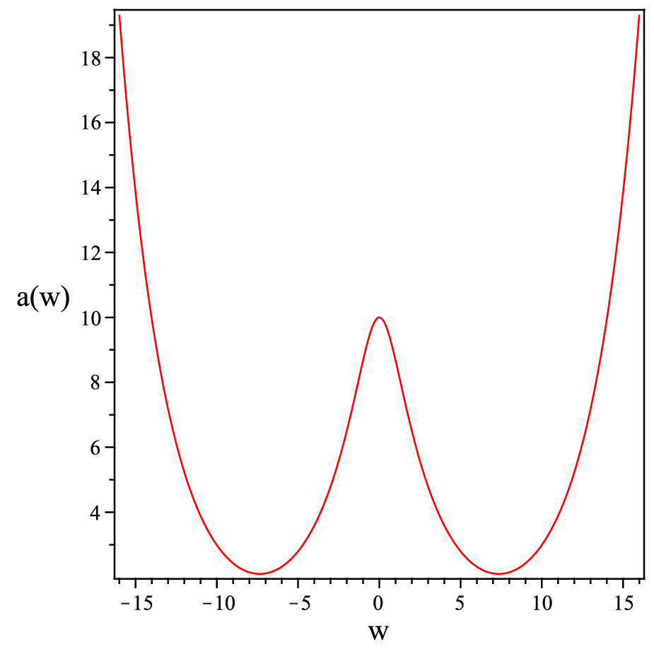
It is obvious that obtaining an exact analytical solution for the above equations is hard. Therefore, at first we try to obtain a numerical solution for the warp functions by assuming the following ansatz for kink like scalar field

ϕ=tanh⁡(w).\phi=\tanh(w). (70)

Inserting Eq. (70) into Eq. (69) and using ODE plot, one can plot Fig. 1 for the warp function in the case of negative λ\lambda.

Figure 1: Numerical plot of warp function in terms of ww for λ=−1\lambda=-1.
Refer to caption

Now, we try to obtain an analytical approximation solution for the large and small values of ww. The corresponding approximate equations are

3a′′a+ϕs′=0,w→0\displaystyle 3\dfrac{a^{{}^{\prime\prime}}}{a}+\phi_{s}^{{}^{\prime}}=0,\hskip 28.45274ptw\rightarrow 0 (71)
3​λ2​a2+ϕl′=0,w→∞.\displaystyle\dfrac{3\lambda}{2a^{2}}+\phi_{l}^{{}^{\prime}}=0,\hskip 28.45274ptw\rightarrow\infty. (72)

and

3a′′2​a+Vs=0,w→0\displaystyle\dfrac{3a^{{}^{\prime\prime}}}{2a}+V_{s}=0,\hskip 28.45274ptw\rightarrow 0 (73)
9​λ4​a2−Vl=0,w→∞.\displaystyle\dfrac{9\lambda}{4a^{2}}-V_{l}=0,\hskip 28.45274ptw\rightarrow\infty. (74)

In order to solve these equations according to Fig. 1 for λ=−1\lambda=-1, we assume the following ansatz for the warp function

a⁡(w)=(w2−α2)2.a(w)=(w^{2}-\alpha^{2})^{2}. (75)

By inserting (75) into Eq. (71), one can get

ϕs\displaystyle\phi_{s} =\displaystyle= 24α​arctan⁡(wα),\displaystyle\dfrac{24}{{\alpha}}\arctan\left(\dfrac{w}{{\alpha}}\right), (76)
ϕl\displaystyle\phi_{l} =\displaystyle= λα6​(w2−α2)3​(α​w​(33​α4−40​α2​w2+15​w4)CLOSE\displaystyle\dfrac{\lambda}{\alpha^{6}(w^{2}-\alpha^{2})^{3}}\left(\alpha w(33\alpha^{4}-40\alpha^{2}w^{2}+15w^{4})\right. (77)
OPEN−15​(w2−α2)3​arctan⁡(wα)).\displaystyle\left.-15(w^{2}-\alpha^{2})^{3}\arctan(\dfrac{w}{\alpha})\right).

and

Vs=\displaystyle V_{s}= 6α2​[3−2​cosh2⁡(α​ϕ)]​cosh2⁡(α​ϕ),\displaystyle\dfrac{6}{\alpha^{2}}\left[3-2\cosh^{2}(\alpha\phi)\right]\cosh^{2}(\alpha\phi), (78)
Vl=\displaystyle V_{l}= 9​λ4​α8​cosh8⁡(α​ϕ).\displaystyle\dfrac{9\lambda}{4\alpha^{8}}\cosh^{8}(\alpha\phi). (79)

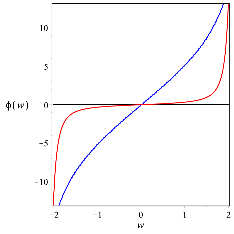
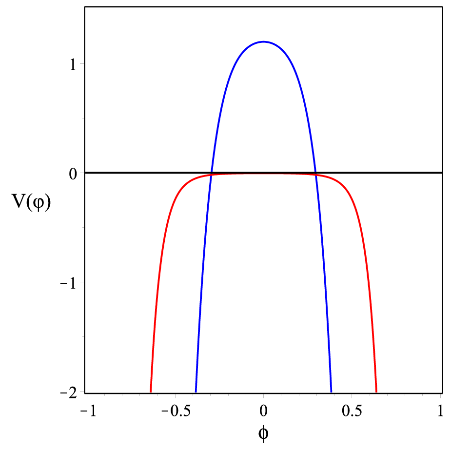
In figures (2), we have plotted the behavior of above functions. As can be seen in the figure (2a), the approximate scalar field has mirror symmetry ϕ⁡(w)=−ϕ⁡(−w)\phi(w)=-\phi(-w). The scalar potential plotted in the Fig. (2a). It can be seen that the potential is an even function of ww (V⁡(w)=V⁡(−w)V(w)=V(-w)), but it is unbounded from below. This is a consequence of choosing the warp function (75) as w4w^{4} when |w|→∞|w|\to\infty.

Refer to caption
Refer to caption
Figure 2: Plot of ϕs\phi_{s} (blue line) and ϕl\phi_{l} (red line) in terms of ww for λ=−1\lambda=-1 and α=5\alpha=5 (left) plot of VsV_{s}(blue line) and VlV_{l} (red line) in terms of ww for λ=−1,α=5\lambda=-1,\alpha=5 (right).

III.2 Case II: ϕ⁡(w,t)=ϕ⁡(t):\phi(w,t)=\phi(t):

By considering a time dependent scalar field, it is straightforward to simplify the relations of Eq. (46) as follow

t​t−c​o​m​p​o​n​e​n​t:\displaystyle tt-component:\hskip 14.22636pt 3a2(a2′+aa′′−b˙2b2−κb2)=−12​a2ϕ˙2−V,\displaystyle\dfrac{3}{a^{2}}\left(a^{{}^{\prime}2}+aa^{{}^{\prime\prime}}-\dfrac{\dot{b}^{2}}{b^{2}}-\dfrac{\kappa}{b^{2}}\right)=-\dfrac{1}{2a^{2}}\dot{\phi}^{2}-V, (80)
i​j−c​o​m​p​o​n​e​n​t:\displaystyle ij-component:\hskip 14.22636pt 1a2(−2b¨b−b˙2b2−κb2+3a2′+3aa′′)=12​a2ϕ˙2−V,\displaystyle\dfrac{1}{a^{2}}\left(-2\dfrac{\ddot{b}}{b}-\dfrac{\dot{b}^{2}}{b^{2}}-\dfrac{\kappa}{b^{2}}+3a^{{}^{\prime}2}+3aa^{{}^{\prime\prime}}\right)=\dfrac{1}{2a^{2}}\dot{\phi}^{2}-V, (81)
w​w−c​o​m​p​o​n​e​n​t:\displaystyle ww-component:\hskip 14.22636pt 3a2​(−b¨b+2​a2′−b˙2b2−κb2)=12​a2​ϕ˙2−V,\displaystyle\dfrac{3}{a^{2}}\left(-\dfrac{\ddot{b}}{b}+2a^{{}^{\prime}2}-\dfrac{\dot{b}^{2}}{b^{2}}-\dfrac{\kappa}{b^{2}}\right)=\dfrac{1}{2a^{2}}\dot{\phi}^{2}-V, (82)
scalar field equation:\displaystyle scalar\text{ }field\text{ }equation:\hskip 14.22636pt ϕ¨+3​b˙b​ϕ˙+a2​∂V∂ϕ=0.\displaystyle\ddot{\phi}+3\dfrac{\dot{b}}{b}\dot{\phi}+a^{2}\dfrac{\partial V}{\partial\phi}=0. (83)

Subtracting Eq. (81) from Eq. (82), we can obtain

b¨b+2​b˙2b2+2​κb2−3a2′+3aa′′=0.\dfrac{\ddot{b}}{b}+\dfrac{2\dot{b}^{2}}{b^{2}}+\dfrac{2\kappa}{b^{2}}-3a^{{}^{\prime}2}+3aa^{{}^{\prime\prime}}=0. (84)

Separation of time-dependent and w−w-dependent terms, we find

b¨b+2​b˙2b2+2​κb2=\displaystyle\dfrac{\ddot{b}}{b}+\dfrac{2\dot{b}^{2}}{b^{2}}+\dfrac{2\kappa}{b^{2}}= c,\displaystyle c, (85)
3a2′−3aa′′=\displaystyle 3a^{{}^{\prime}2}-3aa^{{}^{\prime\prime}}= c,\displaystyle c, (86)

where cc is the separation constant. Now, we can solve Eq. (86) to obtain

a⁡(w)=c1​c​sin⁡(w+c23​c1).a(w)=c_{1}\sqrt{c}\sin\left(\dfrac{w+c_{2}}{\sqrt{3}c_{1}}\right). (87)

in which c1c_{1} and c2c_{2} are two integration constants.

Considering Eqs. (80), (82) and (85), we can find

ϕ˙2=6​(b˙2b2+κb2−c3).\dot{\phi}^{2}=6\left(\dfrac{\dot{b}^{2}}{b^{2}}+\dfrac{\kappa}{b^{2}}-\dfrac{c}{3}\right). (88)

As the final step, we use Eq. (82), to achieve a constant scalar potential as follows

V=−6a′′a=23​c1.V=-\dfrac{6a^{{}^{\prime\prime}}}{a}=\dfrac{2}{3c_{1}}. (89)

which is supported for the flat region of slow-roll inflation. By inserting the above potential in Eq. (83) and applying the slow-roll inflation criteria (ϕ˙≪V,ϕ¨≪3​H​ϕ˙\dot{\phi}\ll V,\ddot{\phi}\ll 3H\dot{\phi}), we can find the initial value for the scalar field ϕ=ϕ0\phi=\phi_{0}.

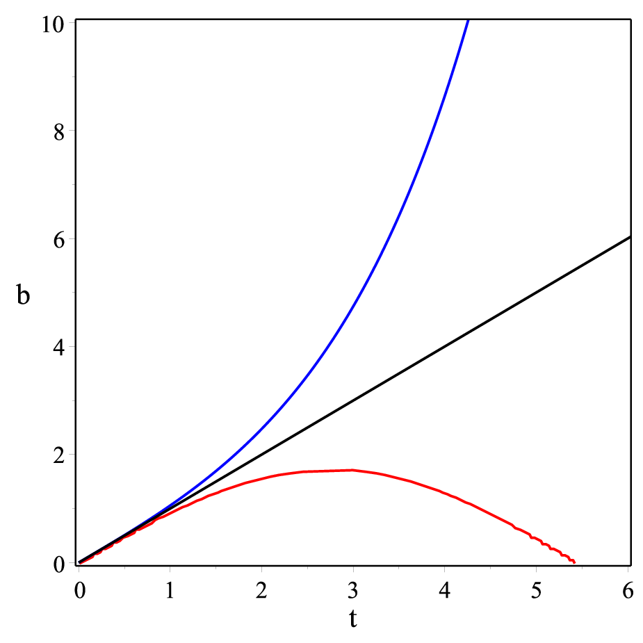
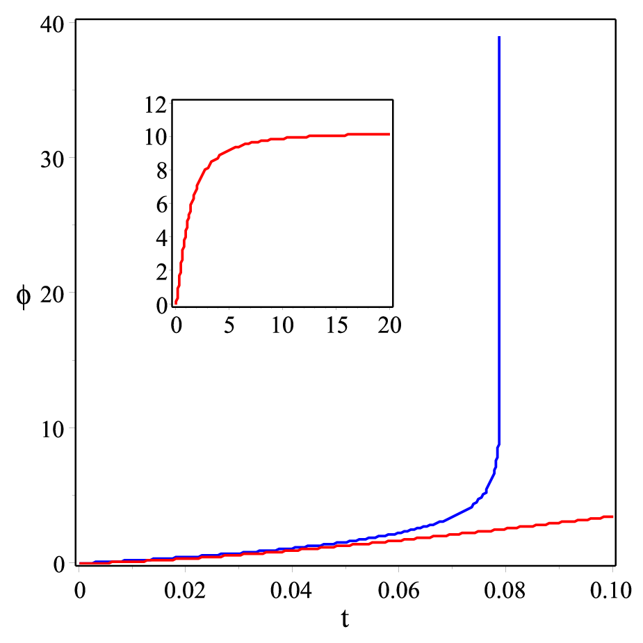
According to Eqs. (85) and (88), we plot Fig. 3 to show the behavior of both the scale factor and scalar field in terms of time for κ=−1\kappa=-1 and different values of cc. According to Eq. (87), only the case of c=1c=1 is acceptable since c=0,−1c=0,-1 leads to zero and imaginary warp functions. As can be seen in figure (3a), the scale factor in terms of time has an inflationary behavior (b∝t2b\propto t^{2}). Also, such a behavior one can see in figure (3b) for scalar field in terms of time. This behavior is similar to the inflaton field in high energy Choudhury:2011sq.
Refer to caption
Refer to caption
Figure 3: Plots of scale factor in terms of tt for κ=−1\kappa=-1 and c=−1c=-1(red line), c=0c=0 (black line) and c=1c=1 (blue line)(left) plots of ϕ\phi in terms of tt for κ=−1,c=1\kappa=-1,c=1 (blue line) and c=−1c=-1 (red line) and in the inset for the large value has been plotted (right).

IV Conclusion

In this paper, we have presented five-dimensional thick brane solutions supported by a scalar field. We have briefly addressed the formalism of canonical gravity and the WD equation as applied to the brane. We have seen that only in the case of κ=−1\kappa=-1, tunneling occurs which means that the appropriate classical cosmology subject to quantization is the spatially paraboloid case.

Then, we studied the cosmology of thick brane for κ=−1\kappa=-1 and in the case of time (in)dependent scalar field. In each case, we have obtained the corresponding solutions of both the scale factor and scalar field. It is worth mentioning that considering a time-dependent scalar field leads to a constant scalar potential which is supported by the known slow-roll inflation.

We also leave the case where ϕ⁡(w,t)=ϕ⁡(w)​φ​(t)\phi(w,t)=\phi(w)\varphi(t) in appendix for future consideration.

Appendix A Case: ϕ⁡(w,t)=ϕ⁡(w)​φ​(t)\phi(w,t)=\phi(w)\varphi(t)

Here we consider the case ϕ⁡(w,t)=ϕ⁡(w)​φ​(t)\phi(w,t)=\phi(w)\varphi(t). By using of scalar field equation (46), we have

φ˙​(t)φ⁡(t)+3​b˙​(t)b⁡(t)​φ˙​(t)φ⁡(t)−\displaystyle\dfrac{\dot{\varphi}(t)}{\varphi(t)}+\dfrac{3\dot{b}(t)}{b(t)}\dfrac{\dot{\varphi}(t)}{\varphi(t)}- (a2ϕ′′(w)ϕ⁡(w)+4aa′ϕ′(w)ϕ⁡(w))=\displaystyle\left(\dfrac{a^{2}\phi^{{}^{\prime\prime}}(w)}{\phi(w)}+4aa^{{}^{\prime}}\dfrac{\phi^{{}^{\prime}}(w)}{\phi(w)}\right)=
−a2φ⁡(t)​ϕ​(w)​∂V∂ϕ⁡(w,t).\displaystyle-\dfrac{a^{2}}{\varphi(t)\phi(w)}\dfrac{\partial V}{\partial\phi(w,t)}. (90)

Also, by adding t​ttt and w​www components of field equations (46), one can obtain

3a2(3a2′+aa′′−b¨b−2​b˙2b2−2​κb2)=−2V.\dfrac{3}{a^{2}}\left(3a^{{}^{\prime}2}+aa^{{}^{\prime\prime}}-\dfrac{\ddot{b}}{b}-\dfrac{2\dot{b}^{2}}{b^{2}}-\dfrac{2\kappa}{b^{2}}\right)=-2V. (91)

In order to solve the field equation (A) and (91), we should separate the equations in terms of tt and ww. To this end, one should consider appropriate choices for V⁡(ϕ)V(\phi). As a simple case we considered V=0V=0. In this case the field equations reduce to

b¨b+2​b˙2b2+2​κb2−c=0\displaystyle\dfrac{\ddot{b}}{b}+\dfrac{2\dot{b}^{2}}{b^{2}}+\dfrac{2\kappa}{b^{2}}-c=0
3a2′+aa′′−c=0\displaystyle 3a^{{}^{\prime}2}+aa^{{}^{\prime\prime}}-c=0 (92)

and

φ¨(t)+3​b˙bφ˙(t)−c′φ(t)=0\displaystyle\ddot{\varphi}(t)+\dfrac{3\dot{b}}{b}\dot{\varphi}(t)-c^{{}^{\prime}}\varphi(t)=0
ϕ′′(w)+4a′aϕ′(w)−c′a2ϕ(w)=0.\displaystyle\phi^{{}^{\prime\prime}}(w)+\dfrac{4a^{{}^{\prime}}}{a}\phi^{{}^{\prime}}(w)-\dfrac{c^{{}^{\prime}}}{a^{2}}\phi(w)=0. (93)

One can solve the equations (A) for warp function and scale factor and then insert them in to the equations (A) obtain the scalar fields.

References

  • (1) T. Kaluza, Sitz. Preuss. Akad. Wiss. Phys. Math. K 1. 966 (1921).
  • (2) L. Randall and R. Sundrum, Phys. Rev. Lett. 83, 3370 (1999).
  • (3) N. Arkani-Hamed, S. Dimopoulos and G. Dvali, Phys. Lett. B 429, 263 (1998).
  • (4) I. Antoniadis, S. Dimopoulos and G. Dvali, Nucl. Phys. B 516, 70 (1998).
  • (5) L. Randall and R. Sundrum, Phys. Rev. Lett. 83, 4690 (1999).
  • (6) J. Garriga and T. Tanaka, Phys. Rev. Lett. 84, 2778 (2000).
  • (7) S. B. Giddings, E. Katz and L. Randall, JHEP 0003, 023 (2000).
  • (8) O. DeWolfe, D. Z. Freedman, S. S. Gubser and A. Karch, Phys. Rev. D 62, 046008 (2000).
  • (9) M. Gremm, Phys. Lett. B 478, 434 (2000).
  • (10) C. Csaki, J. Erlich, T. J. Hollowood and Y. Shirman, Nucl. Phys. B 581, 309 (2000).
  • (11) A. Kehagias and K. Tamvakis, Phys. Lett. B 504, 38 (2001).
  • (12) M. Gremm, Phys. Rev. D 62, 044017 (2000).
  • (13) V. Dzhunushaliev, Grav. Cosmol. 13, 302 (2007).
  • (14) V. Dzhunushaliev, V. Folomeev, S. Myrzakul and R. Myrzakulov, Mod. Phys. Lett. A 23, 2811 (2008).
  • (15) M. Gremm, Phys. Lett. B 478, 434 (2000).
  • (16) A. Wang, Phys. Rev. D 66, 024024 (2002).
  • (17) D. Bazeia, F. A. Brito and J.R. Nascimento, Phys. Rev. D 68, 085007 (2003).
  • (18) D. Bazeia, C. Furtado and A. R. Gomes, JCAP 0402, 002 (2004).
  • (19) S. Kobayashi, K. Koyama and J. Soda, Phys. Rev. D 65, 064014 (2002).
  • (20) A. Melfo, N. Pantoja and A. Skirzewski, Phys. Rev. D 67, 105003 (2003).
  • (21) C. Barcel´o, C. Germani and C.F. Sopuerta, Phys. Rev. D 68, 104007 (2003).
  • (22) H. Guo, Y.-X. Liu, S.-W. Wei and C.-E. Fu, Europhys. Lett. 97, 60003 (2012).
  • (23) K.A. Bronnikov and B.E. Meierovich, Grav. Cosmol. 9, 313 (2003).
  • (24) A. Karch, L. Randall, JHEP, 0105, 008 (2001).
  • (25) P. D. Mannheim, Brane-localized Gravity, (World Scientific Publishing Company, Singapore) 2005; SenGupta S., Aspects of warped brane world models, arXiv:0812.1092[hep-th].
  • (26) J. A. Wheeler, Ann. Phys. (N.Y.) 2, 604 (1957).
  • (27) B. S. DeWitt, Phys. Rev. 160, 1113 (1967).
  • (28) J. B. Hartle, S. W. Hawking, Phys. Rev. D 28, 2960 (1983).
  • (29) S. W. Hawking, Nucl. Phys. B 239, 257 (1984).
  • (30) S. W. Hawking, D. N. Page, Nucl. Phys. B 264, 185 (1986).
  • (31) J. J. Halliwell, S. W. Hawking, Phys. Rev. D 31, 1777 (1985).
  • (32) A. Vilenkin, Phys. Lett. B 117, 25 (1982).
  • (33) A. Vilenkin, Phys. Rev. D 27, 2848 (1983).
  • (34) A. Vilenkin, Phys. Rev. D 30, 549 (1984).
  • (35) A. Vilenkin, Phys. Rev. D 37, 888 (1988).
  • (36) F. Darabi, W. N. Sajko and P. S. Wesson, Class. Quant. Grav. 17, 4357 (2000).
  • (37) S. H. Hendi, N. Riazi and S. N. Sajadi, Phys. Rev. D 102, no.12, 124034 (2020).
  • (38) A. Ahmed, B. Grzadkowski and J. Wudka, JHEP 1404, 061 (2014).
  • (39) A. Wang, Phys. Rev. D 66, 024024 (2002).
  • (40) V. Dzhunushaliev, V. Folomeev and M. Minamitsuji, Rept. Prog. Phys. 73, 066901 (2010).
  • (41) S. Choudhury and S. Pal, Phys. Rev. D 85, 043529 (2012).