Revisiting Andromeda’s ParachuteThanks: Tables 2, 4, 6, and 7 are only available in electronic form at the CDS via anonymous ftp to cdsarc.u-strasbg.fr (130.79.128.5) or via http://cdsweb.u-strasbg.fr/cgi-bin/qcat?J/A+A/vol/page
Abstract
The gravitational lens system PS J0147+4630 (Andromeda’s Parachute) consists of four quasar images ABCD and a lensing galaxy. We obtained -band light curves of ABCD in the 20172021 period from a monitoring with two 2-m class telescopes. These curves and state-of-the-art curve-shifting algorithms led to three independent time delays relative to image A, one of which is accurate enough (uncertainty of about 4%) to be used in cosmological studies. Our finely sampled light curves and some additional fluxes in the years 20102013 also demonstrated the presence of significant microlensing variations. This paper also focused on new near-IR spectra of ABCD in 20182019 that were derived from archive data of two 10-m class telescopes. We analysed the spectral region including the Mg ii, H, [O iii], and H emission lines (0.92.4 m), measuring image flux ratios and a reliable quasar redshift of 2.357 0.002, and finding evidence of an outflow in the H emission. In addition, we updated the lens mass model of the system and estimated a quasar black-hole logarithmic mass = 9.34 0.30.
Key Words.
gravitational lensing: strong – quasars: individual: PS J0147+46301 Introduction
Optical frames from the Panoramic Survey Telescope and Rapid Response System (Chambers et al. 2019, Pan-STARRS;) led to the serendipitous discovery of the strong gravitational lens system with a quadruply-imaged quasar (quad) PS J0147+4630 (Berghea et al. 2017). Due to its position in the sky and the spatial arrangement of the four quasar images, this quad is also called Andromeda’s Parachute (Rubin et al. 2018, e.g.). The three brightest images (A, B and C) forms an arc that is about 3″ from the faintest image D, and the main lens galaxy G is located between the bright arc and D. This configuration is clearly seen in the left panel of Figure 1, which is based on Hubble Space Telescope (HST) data.
As far as we know, the quasar PS J0147+4630 is the brightest source in the sky at redshifts ¿ 1.4 (apart from transient events such as gamma-ray bursts), and its four optical images can be easily resolved with a ground-based telescope in normal seeing conditions. Thus, it is a compelling target for various physical studies based on high-resolution spectroscopy (Rubin et al. 2018, e.g.) and detailed photometric monitoring (Lee 2018, e.g.). Early two-season monitoring campaigns with the 2.0 m Liverpool Telescope (Goicoechea & Shalyapin 2019, LT;) and the 2.5 m Nordic Optical Telescope (Dyrland 2019, NOT;) provided accurate optical light curves of all quasar images, as well as preliminary time delays and evidence of microlensing-induced variations. A deeper look at the optical variability of Andromeda’s Parachute is of great importance, since robust time delays and well-observed microlensing variations can be used to determine cosmological parameters (Treu & Marshall 2016, e.g.) and the structure of the quasar accretion disc (Schmidt & Wambsganss 2010, e.g.).
Early optical spectra of the system confirmed the gravitational lensing phenomenon and revealed the broad absorption-line (BAL) nature of the quasar (Lee 2017; Rubin et al. 2018). However, there is an appreciable discrepancy between the quasar redshift reported by Rubin et al. 2018 and that measured by Lee 2017, amounting to 0.04. Lee 2018 also performed the first attempt to determine the redshift of G from spectroscopic observations with the 8.1 m Gemini North Telescope (GNT). An accurate reanalysis of these GNT data showed that the first estimate of the lens redshift was biased, by enabling better identification of G as an early-type galaxy at = 0.678 0.001 with stellar velocity dispersion = 313 14 km s-1 (Goicoechea & Shalyapin 2019). Both redshifts, and , are key pieces of information to interpret, among other things, time delays and microlensing effects. Additionally, HST high-resolution imaging of the lens system provided a lens mass model (Shajib et al. 2019; Shajib et al. 2021). To ensure proper interpretation of delays and microlensing-induced phenomena, a reliable lens mass model is also required.

New spectroscopic observations in the unexplored near-IR region are also useful tools to shed light on physical properties of the quad. In addition to the determination of redshifts, wavelength-domain data are often used to measure image flux ratios for emission lines and their underlying continua. These measurements provide insights about the macrolens flux ratios and extinction/microlensing effects (Motta et al. 2012; Goicoechea & Shalyapin 2016; Shalyapin & Goicoechea 2017, e.g.). The macrolens flux ratios, for instance, put constraints on the distribution of mass lensing the quasar. Moreover, if one has information on the magnification and transmission factors for a given quasar image, line widths and continuum fluxes for such image yield estimates of the quasar black hole mass (Vestergaard & Peterson 2006; Assef et al. 2011, e.g.), thus constraining the size of the innermost region in the accretion disc.
| Star | RA(J2000) | Dec(J2000) | |||
|---|---|---|---|---|---|
| PSF | 26.773246 | 46.506670 | 16.366 | 15.606 | 15.260 |
| Control | 26.746290 | 46.504028 | 15.800 | 15.421 | 15.269 |
| Cal1 | 26.805695 | 46.522834 | 16.587 | 16.292 | 16.208 |
| Cal2 | 26.725610 | 46.488113 | 16.857 | 16.405 | 16.257 |
| Cal3 | 26.752831 | 46.518659 | 17.157 | 16.836 | 16.718 |
| Cal4 | 26.760809 | 46.474513 | 17.229 | 16.856 | 16.714 |
| Cal5 | 26.824027 | 46.528718 | 15.656 | 15.200 | 15.029 |
| Cal6 | 26.790480 | 46.502241 | 15.145 | 14.831 | 14.716 |
This paper is organized as follows. In Sect. 2, we present combined LT and NOT light curves of the four images of PS J0147+4630 spanning four observing seasons from 2017 to 2021. In Sect. 3, using these optical light curves, we carefully analyse the time delays between images and the quasar microlensing variability. In Sect. 4, we present an analysis of near-IR spectroscopic data of the system in 20182019, focusing on the quasar redshift and the image flux ratios. In Sect. 5, assuming a flat CDM (standard) cosmology, we discuss the Hubble constant () value that is inferred from the lens mass model based on HST imaging, updated redshifts, and the longest time delay that we measure. A lens mass modelling based on astrometric and time-delay constraints is also discussed in Sect. 5. In Sect. 6, we measure the mass of the central black hole in the quasar. Our main conclusions are included in Sect. 7.
2 New optical light curves
We monitored PS J0147+4630 with the LT from 2017 August to 2021 February using the IO:O optical camera with a pixel scale of 030. Each observing night, a single 120 s exposure was taken in the Sloan -band filter, and over the full monitoring period, 145 -band frames were obtained. The LT data reduction pipeline carried out three basic tasks: bias subtraction, overscan trimming, and flat fielding. Additionally, the IRAF software22 2 https://iraf-community.github.io/ (Tody 1986; Tody 1993) allowed us to remove cosmic rays and bad pixels from all frames. We extracted the brightness of the four quasar images ABCD through PSF fitting, using the IMFITFITS software (McLeod et al. 1998) and following the scheme described by Goicoechea & Shalyapin 2019. Table 1 includes the position and magnitudes of the PSF star, as well as of other relevant field stars. These data are taken from the Data Release 1 of Pan-STARRS33 3 http://panstarrs.stsci.edu (Flewelling et al. 2020). Our photometric model consisted of four point-like sources (ABCD) and a de Vaucouleurs profile convolved with the empirical PSF (lensing galaxy G). Positions of components with respect to A and structure parameters of G were constrained from HST data (Shajib et al. 2019; Shajib et al. 2021).
We also selected six non-variable blue stars in the field of PS J0147+4630 and performed PSF photometry on five of them (see the calibration stars Cal1-Cal5 in Table 1; Cal6 is a saturated star in LT frames). For each of the five calibration stars, we calculated its average magnitude within the monitoring period and magnitude deviations in individual frames (by subtracting average). In each individual frame, the five stellar magnitude deviations were averaged together to calculate a single magnitude offset, which was then subtracted from the magnitudes of quasar images. After this photometric calibration, we removed 15 observing epochs in which quasar magnitudes deviate appreciably from adjacent values. Thus, the final LT -band light curves are based on 130 frames (epochs), and the typical uncertainties in the light curves of the quasar images and control star (see Table 1) were estimated from magnitude differences between adjacent epochs separated by no more than 4 d (Goicoechea & Shalyapin 2019). We derived typical errors of 0.0058 (A), 0.0069 (B), 0.0091 (C), 0.0188 (D), and 0.0054 (control star) mag. For the control star, we have also verified that its typical error practically coincides with the standard deviation of all measures (0.0051 mag). To obtain photometric uncertainties at each observing epoch, the typical errors were scaled by the relative signal-to-noise ratio of the PSF star (Howell 2006).
The optical monitoring of PS J0147+4630 with the NOT spanned from 2017 August to 2019 December. We used the ALFOSC camera with a pixel scale of 021 and the -Bessel filter. This passband is slightly redder than the Sloan band. Each observing night, we mainly took three exposures of 30 s each under good seeing conditions. The full-width at half-maximum (FWHM) of the seeing disc was about 1″, and we collected 298 individual frames over the entire monitoring campaign. After a standard data reduction, IMFITFITS PSF photometry yielded magnitudes for the quasar images (see above for details on the photometric model). To avoid biases in the combined LT-NOT light curves, the same photometric method was applied to LT and NOT frames. This method differs from that of Dyrland 2019, who used the DAOPHOT package in IRAF (Stetson 1987; Massey & Davis 1992) to extract magnitudes from NOT frames.
The six calibration stars in Table 1 were used to adequately correct quasar magnitudes (see above), and we were forced to remove 17 individual frames leading to magnitude outliers. We then combined -band magnitudes measured on the same night to obtain photometric data of the lensed quasar and control star at 77 epochs. Again, typical errors were derived from magnitudes at adjacent epochs that are separated 4.5 d. This procedure led to uncertainties of 0.0122 (A), 0.0122 (B), 0.0144 (C), 0.0197 (D), and 0.0170 (control star) mag. Errors at each observing epoch were calculated in the same way as for the LT light curves.
As a last step, we combined the -band LT and -band NOT light curves. If we focus on the quasar images and consider pairs separated by no more than 2.5 d, the values of the average colour are 0.0568 (A), 0.0619 (B), 0.0549 (C), and 0.0655 (D). Brightness records of the ABC images are more accurate than those of D, and thus we reasonably take the average colours of ABC to estimate a mean offset of 0.0579 mag. After correcting the -band curves of the quasar for this offset, we obtain the new records in Table 2. This machine-readable ASCII file at the CDS contains -band magnitudes of the quasar images and the control star at 207 observing epochs (MJD50 000). In Figure 1, we also display our new 4-year light curves.
3 Time delays and microlensing signals


Previous efforts focused on early monitorings with a single telescope, trying to estimate delays between the image A and the other quasar images, (X = B, C, D), and find microlensing signals (Dyrland 2019; Goicoechea & Shalyapin 2019)44 4 Goicoechea & Shalyapin 2019 used the notation rather than that defined in this paper and Dyrland 2019. Here, we use the new light curves in Section 2 along with state-of-the-art curve-shifting algorithms to try to robustly measure the three independent time delays , , and . At the end of this section, we also discuss the intrinsic and extrinsic (microlensing) variability of the quasar.
There are several cross-correlation techniques to measure time delays between light curves containing microlensing variations (e.g. Liao et al. 2015, and references therein), and thus we considered two very different methods and models to obtain reliable results. First, we performed the AB, AC, and AD comparisons using the dispersion method (Pelt et al. 1996). This technique evaluates the dispersion between two different light curves for a range of time lags and flux-ratio model parameters. For given values of the time lag and model parameters, each data point in one of the two light curves is compared with magnitudes in the other curve at time separations shorter than a decorrelation length , and squared differences between pairs of data with longer separations and larger photometric errors have smaller weights. The key idea of the method is to find the time lag and model parameters that minimises the dispersion, i.e. the weighted sum of squared differences.
Our flux ratio model accounted for microlensing variability by incorporating four magnitude offsets instead a single one. In order to match the light curve of the reference image A and the shifted curve of another quasar image, the curve of A was splitted into four one-year segments, covering one observing season each. We then assumed a constant magnitude offset within every segment, while the offset was allowed to vary from one segment to other. This seasonal magnitude offset (SMO) model works well in presence of intra-year microlensing events and microlensing variability on timescales of several years (Goicoechea & Shalyapin 2016; Shalyapin et al. 2021). We have written a Python code to minimise the (AB), (AC), and (AD) dispersions, and used three reasonable values of 10, 15 and 20 d. This 10-d interval of permits us to account for the intrinsic variance of the technique. Figure 2 displays the three dispersion spectra for the AD comparison.
We also carried out 1000 ”repetitions of the experiment” by generating 1000 synthetic light curves of each image, peforming AB, AC, and AD comparisons from these simulated curves, and obtaining the distributions of time lags and magnitude offsets that minimise dispersions (e.g. Goicoechea & Shalyapin 2019, and references therein). For example, the 1 confidence intervals for through the corresponding time lag distributions are: 166.1 9.5, 166.3 8.5, and 166.3 8.4 d for = 10, 15, and 20 d, respectively. These measurements indicate that the intrinsic variance is well below the uncertainties, so hereafter we show only results for = 15 d. The 1 confidence intervals for , , and are listed in Table 3.
| Method/model | |||
|---|---|---|---|
| /SMO | 1.0 1.8 | +4.5 3.6 | 166.3 8.5 |
| /FKS | 0.9 4.2 | +5.4 4.4 | 168.7 6.2 |
| Combined | 0 3 | +5 4 | 167.5 7.4 |
Note: When applying the dispersion, we consider a SMO model without assumptions about the intrinsic variability. We also use the technique along with a FKS model to describe the intrinsic and extrinsic variations. Additionally, we combine /SMO and /FKS delays in a simple way, i.e. calculating mean central values and mean errors. We adopt these averages for subsequent studies. Here, (X = B, C, D) are in days, image A leads image X if 0 (otherwise A trails X), and all measurements are 68% confidence intervals.
Second, the time delays of PS J0147+4630 were inferred from PyCS3 curve-shifting algorithms55 5 https://gitlab.com/cosmograil/PyCS3 (Tewes et al. 2013; Millon et al. 2020a; Millon et al. 2020b). PyCS3 is a software toolbox to estimate time delays between images of gravitationally lensed quasars, and we focused on the technique, assuming that the intrinsic signal and the extrinsic ones can be modelled as a free-knot spline (FKS). This technique shifts the four light curves simultaneously (ABCD comparison) to better constrain the intrinsic variability, and relies on an iterative nonlinear procedure to fit the four time shifts and splines that minimise the between the data and model (Tewes et al. 2013). Results depend on the initial guesses for the time shifts, so it is necessary to estimate the intrinsic variance of the method using a few hundred initial shifts randomly distributed within reasonable time intervals. In addition, a FKS is characterised by a knot step, which represents the initial spacing between knots. The model consists of an intrinsic spline with a knot step and four independent extrinsic splines with that account for the microlensing variations in each quasar image (Millon et al. 2020b).
To address the intrinsic variability, we considered three values of 30, 50 and 70 d. Intrinsic knot steps shorter than 30 d fit the observational noise, whereas values longer than 70 d do not fit the most rapid variations of the source quasar. Intrinsic variations are usually faster than extrinsic ones, and additionally, the software works fine when the microlensing knot step is significantly longer than . Therefore, the microlensing signals were modelled as free-knot splines with = 350400 d (Millon et al. 2020b, i.e. values intermediate between those shown in Table 2 of). We also generated 500 synthetic (mock) light curves of each quasar image, optimised every mock ABCD dataset, and checked the similarity between residuals from the fits to the observed curves and residuals from the fits to mock curves. The comparison of residuals was made by means of two statistics: standard deviation and normalised number of runs (Tewes et al. 2013, see details in). For = 50 d and = 400 d, histograms of residuals derived from mock curves (grey) and from the LT-NOT light curves of PS J0147+4630 are included in the top panels of Figure 3. It is apparent that the standard deviations through the synthetic and the observed curves match very well. Additionally, the bottom panels of Figure 3 show distributions of from synthetic light curves (grey) for = 50 d and = 400 d. These bottom panels also display the values from the observations (vertical lines), which are typically located at 0.3 of the mean values of the synthetic distributions.
Four pairs of (, ) values (see above) led to the set of time delays in Figure 4. We have verified that other feasible choices for (e.g. = 200 d) do not substantially modify the results in this figure. The black horizontal bars correspond to 1 confidence intervals after a marginalisation over results for all pairs of knot steps, and those in the left panels of Figure 4 are included in Table 3. We finally adopted the time delays in the fourth row of Table 3, which were obtained by averaging central values and errors in the two previous rows. It seems to be difficult to accurately determine delays between the brightest images ABC because they are really short. To robustly measure and in a near future, we will most likely need to follow a non-standard strategy focused on several time segments associated with strong intrinsic variations and weak extrinsic signals. Fortunately, we find an accurate and reliable value of (uncertainty of about 4%), confirming the early result by Dyrland 2019.

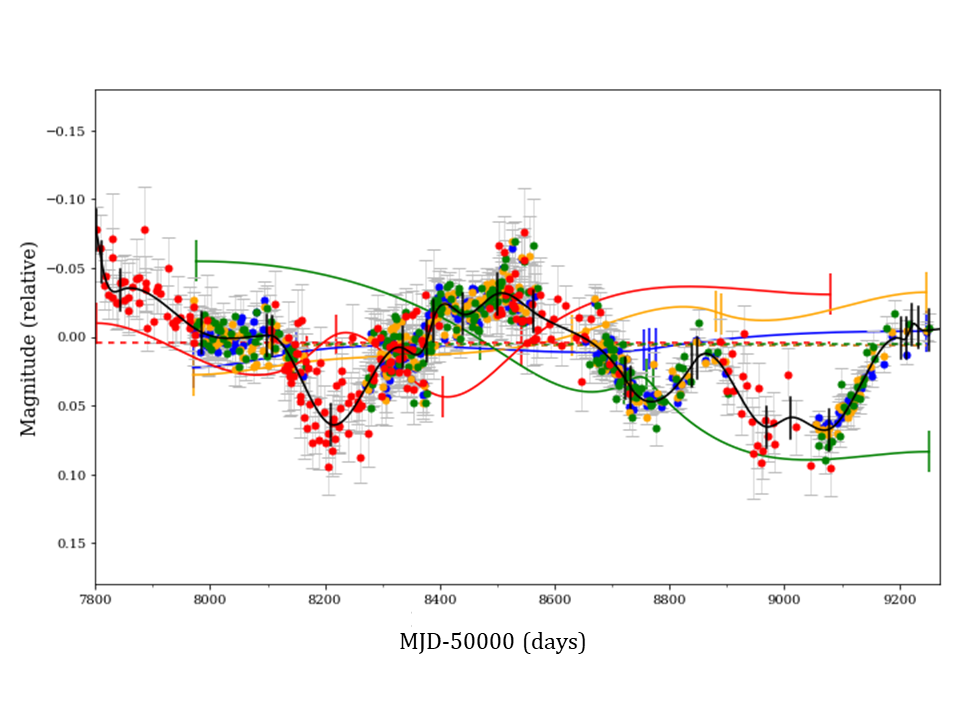


After building median-subtracted light curves, the central values of the adopted time delays (see Table 3) were used to shift in time such normalised curves. As A is the reference image and = 0, the new curves of A and B retained their original epochs. We then applied the PyCS3 software (/FKS model) to simultaneously fit the intrinsic signal and the microlensing variability of each quasar image. Figure 5 displays our results for = 30 d and = 400 d (left panel), and = 70 d and = 200 d (right panel). The black lines with knot vertical ticks model the intrinsic variation shared by the four light curves. Both intrinsic signal reconstructions are compared with microlensing-corrected and time-shifted normalised curves (circles). The blue, orange, green, and red lines model the microlensing variations of A, B, C, and D, respectively. The A image is weakly affected by microlensing, while the other three images show microlensing episodes with total amplitudes exceeding 0.05 mag, and the extrinsic variation of C is particularly prominent. We note that the two pairs of (, ) values we use in Figure 5 lead to similar delays between A and D (both consistent with the adopted one), but they produce microlensing splines for D (red lines) having different behaviours on time scales of hundreds of days.
| Emission | ||||
|---|---|---|---|---|
| Mg ii | 2.355 | 0.065 0.001 | ||
| cont@2800 | 0.113 0.001 | |||
| H | 0.450 0.012 | 0.263 0.010 | 0.065 0.003 | |
| [O iii] | 2.357 | |||
| [O iii] | 0.559 0.038 | 0.311 0.037 | 0.072 0.017 | |
| cont@5100 | 0.593 0.012 | 0.423 0.008 | 0.122 0.005 | |
| H main | 2.359 | 0.484 0.003 | 0.292 0.002 | 0.064 0.001 |
| H VBC | 0.541 0.007 | 0.406 0.005 | 0.068 0.003 | |
| cont@6563 | 0.636 0.002 | 0.435 0.001 | 0.152 0.001 |
Note: The Mg ii and cont@2800 (continuum at = 2800 Å) emissions are derived from the multi-component decomposition of Keck-ESI spectra (see the right panel of Figure 7). The H, [O iii], cont@5100 (continuum at = 5100 Å), H, and cont@6563 (continuum at = 6563 Å) emissions are inferred from multi-component decompositions of GTC-EMIR spectra (see Figures 10 and 11).
We also considered the adopted time delays to fit seasonal magnitude offsets between image A and the other three images (/SMO model). In the left panel of Figure 6, we show the overlaps between the A data and the magnitude- and time-shifted curves of BCD. It is noteworthy that there is a significant overlap between the original curve of A and the shifted curve of D (see also Figure 5), supporting the reliability of the measurements in Table 3. In addition to an image comparison spanning four years, a comparison over an 11-year period is depicted in the right panel of Figure 6. We have downloaded five -band warp frames of PS J0147+4630 that are included in the Data Release 2 of the Pan-STARRS. These Pan-STARRS frames were obtained on three nights in the 20102013 period, i.e. a few years before the discovery of the lens system. Two frames are available on two of the three nights, so rough photometric uncertainties through average intranight variations are 0.012 (A), 0.008 (B), 0.019 (C), and 0.033 (D) mag. To discuss the differential microlensing variability of the images BCD with respect to A, the right panel of Figure 6 shows the original curve of A along with shifted curves of BCD. We used the adopted time delays and arbitrary (constant) magnitude offsets to shift curves. The shapes of the four brightness records indicate the presence of long-term microlensing effects and suggest that PS J0147+4630 is a suitable target for a deeper analysis of its microlensing signals.
4 Quasar redshift and image flux ratios from recent spectroscopic data
Rubin et al. 2018 estimated the redshift of PS J0147+4630 by cross-correlating a quasar spectral template with spectra of the four quasar images at wavelengths shorter than 5500 Å. This blue spectral region contains emission lines that are severely affected by absorption features, and even excluding the Ly and N v lines, Rubin et al. obtained an inaccurate redshift = 2.377 0.007 for the BAL quasar. The C iii] emission of the broad absorption-line quasar is observed at 6400 Å, and Lee 2017 measured = 2.341 0.001 using only such emission line, which is apparently free of significant absorption-induced distortions. In this section, we analyse several emission lines at longer wavelengths, checking the reliability of the current value of and trying to get information on image flux ratios.
The Keck Observatory Archive includes relevant data of PS J0147+4630 on 1 December 2018 (MJD50 000 = 8453)66 6 https://koa.ipac.caltech.edu/cgi-bin/KOA/nph-KOAlogin (Program ID: U122, Program PI: C. Fassnacht). These deep spectroscopic observations with the Echellette Spectrograph and Imager (Sheinis et al. 2002, ESI;) consisted of 32400 s exposures using an 10-width slit with a spatial pixel scale of 0154. The slit was oriented along the line joining A and D. In addition, the ESI wavelength range and its resolving power were 390010 500 Å and 4000, respectively. We downloaded the exposures of the lens system and spectroscopic data of the standard star Feige110, as well as CuAr, Xe, and HgNe lamps exposures for wavelength calibration. Data reduction and spectral extraction were then performed using the MAuna Kea Echelle Extraction (MAKEE) package by Tim Barlow77 7 https://sites.astro.caltech.edu/~tb/makee. To extract the individual spectra of A and D from the MAKEE software, we considered two apertures with 7 pixel size, which are similar to the slit width and the FWHM seeing. The normalised spectrum of the standard star allowed us to calibrate in flux and correct by telluric absorption the quasar spectra.
The final spectra of A and D are available in tabular format at the CDS: Table 4 includes fluxes of both quasar images covering the spectral range 390010 500 Å with 33 001 channels of 0.2 Å each. The Keck-ESI spectra of the two images are also plotted in the left panel of Figure 7. These new spectra show emission lines that were previously detected at visible wavelengths (Lee 2017; Rubin et al. 2018) and the Mg ii line at 9400 Å. Thus, we focused on the analysis of the Mg ii line spectral region using a decomposition into three components: power-law continuum, Fe ii pseudo-continuum, and Gaussian Mg ii emission (see the right panel of Figure 7). The two Gaussian distributions (A and D) led to an unbiased redshift = 2.355. Additionally, the flux ratios for the pure Mg ii emission and the continuum at = 2800 Å are given in Table 5. Uncertainties in these flux ratios (1 confidence intervals) were estimated from 300 repetitions of each spectrum. To obtain synthetic spectra for A and D, we modified the observed fluxes by adding realizations of normal distributions around zero, with standard deviations equal to the measured errors.
Recent spectroscopic observations of PS J0147+4630 with the near-IR instrument EMIR (Garzón et al. 2016) on the 10.4 m Gran Telescopio Canarias (GTC) are useful tools to discuss the H, [O iii], and H emissions from the distant quasar. These data were taken on 14 August 2019 (MJD50 000 = 8709) under excellent seeing conditions (FWHM seeing 06) and are available at the GTC Public Archive88 8 https://gtc.sdc.cab.inta-csic.es/gtc/ (Program ID: GTCMULTIPLE2B-19B, Program PI: R. Scarpa). The 06-width slit was oriented along two different directions (see Figure 8): one crossing the ABC images (slit orientation 1; total exposure time of 1920 s = 12160 s), and the other crossing the AD images and the lens galaxy G (slit orientation 2; total exposure time of 3840 s = 24160 s). The spatial pixel scale was 01915, while the EMIR- pseudo-grism wavelength range and resolving power were 1.452.42 m and 987, respectively. There are also observations of the standard telluric star HIP10814 on the same night.


We downloaded the GTC-EMIR data and used the PyEMIR software (Cardiel et al. 2019) for their reduction. For each slit orientation, we extracted three individual spectra (ABC or ADG) by fitting three 1D Moffat profiles in the spatial direction for each wavelength bin (Sluse et al. 2007; Shalyapin & Goicoechea 2017; Goicoechea & Shalyapin 2019, e.g.). To fit the Moffat profiles, the positions of BCDG with respect to A were set from the HST astrometry of the system (Shajib et al. 2019; Shajib et al. 2021). Spectra were calibrated in flux, and telluric absorption was properly corrected. In addition, we have taken into account slit losses (relative to A) of 0.928 (B), 0.932 (C), and 0.995 (D) because the BCD images are not centred on the slit axis (see Figure 8). An 1D Moffat profile does not account for the total light of the very faint galaxy G and the slit loss of G is not taken into account either. In this study, we are interested in the quasar spectra and warn that fluxes of G are underestimated. Final spectra for the slit orientations 1 and 2 are shown in Tables 6 and 7, respectively. Both tables are available at the CDS and are structured in a similar way. Table 6 includes wavelengths in Å and fluxes of ABC, whereas Table 7 includes the same wavelengths and fluxes of ADG. All fluxes are given in 10-17 erg cm-2 s-1 Å-1. Figure 9 also displays the new near-IR spectra of PS J0147+4630.
The GTC-EMIR quasar spectra cover the wavelength range of H, [O iii], and H emission lines. At around 4900 Å, these spectra were modelled as the sum of a power-law continuum, a Fe ii pseudo-continuum, and three Gaussian emissions of H, [O iii], and [O iii] (see Figure 10). From the [O iii] doublet, we determined the optimal redshift = 2.357. Flux ratios were also estimated and incorporated in Table 5. To account for the shape of the H emission at rest-frame wavelengths around 6500 Å, we considered a decomposition into three components: power-law continuum and two Gaussian H emissions (see Figure 11), i.e. a main component (the average FWHM of the velocity distributions is 4900 km s-1) and a very broad component (VBC; the average FWHM velocity is 22 300 km s-1) that is blueshifted with respect to the main one by 50009000 km s-1. The source redshift from the main component and several flux ratios are shown in Table 5. Uncertainties in flux ratios from GTC-EMIR data were derived from 300 repetitions of the experiment (synthetic spectra based on the observed ones; see above). To generate simulated spectra of a quasar image, we previously estimated spectral errors as absolute differences between the measured fluxes and those in a smoothed version of its observed spectrum.
Our detailed analysis of emission lines detected at near-IR wavelengths suggests that = 2.357 0.002 (see Table 5). This is basically the average of previous redshifts based on visible spectra, and reported by Lee 2017 and Rubin et al. 2018. The single-epoch image flux ratios in Table 5 are also worthy of attention. We find that all flux ratios for emission lines are smaller than those for continuum emissions at wavelengths inside or near wavelength ranges of lines. Lee 2018 also indicated that the flux ratio for the C iii] emission line is smaller than that for its underlying continuum. This previous result, which was interpreted as evidence of spectral microlensing, is fully consistent with new data in the last column of Table 5. Additionally, the VBC H emission is most likely due to an outflow in the BAL quasar, which is not detected in the H emission. We also note that possible extended blue wings of the [O iii] lines cannot be resolved with available observations. Our data suggest a possible link between the outflow related to absorption features in high-ionization emission lines (Rubin et al. 2018, Ly, N v and C iv;) and the VBC H emission.
At the end of Section 5, flux ratio measurements in Table 5 are compared with macrolens flux ratios predicted by an updated lens mass model, which permits us to discuss extinction/microlensing scenarios. Some results of this discussion are used to confidently estimate the quasar black hole mass in Section 6.
5 Lens mass model
Berghea et al. 2017 presented preliminary modelling of the lens mass of PS J0147+4630 from Pan-STARRS data, whereas Shajib et al. 2019; Shajib et al. 2021 have recently modelled the lens system using HST imaging. Shajib et al.’s solution for the lensing mass relies on a lens scenario consisting of a singular power-law ellipsoid (SPLE; describing the gravitational field of the main lens galaxy G) and an external shear (ES; accounting for the gravitational action of other galaxies). The dimensionless surface mass density (convergence) profile of the SPLE was characterised by a power-law index , and they found = 2.00 0.05, where = 2 for an isothermal ellipsoid99 9 More precisely, the original name of the power-law index in Shajib et al. 2019; Shajib et al. 2021 was , but we have renamed it as to avoid confusion between such index and the shear.
Assuming a flat CDM cosmology with matter and dark energy densities of = 0.3 and = 0.7, respectively1010 10 Results do not change appreciably for values of and slightly different from those adopted here, we first considered Shajib et al.’s solution, updated redshifts = 0.678 (Goicoechea & Shalyapin 2019) and = 2.357 (see Section 4), and our longest (most accurate) time delay in the fourth row of Table 3 to calculate and put it into perspective (Jackson 2015, e.g.). Using the measured delay between images A and D, the Hubble constant is 102 11 km s-1 Mpc-1, in clear disagreement with currently accepted values around = 70 km s-1 Mpc-1. If additional mass along the line of sight is modelled as an external convergence , the factor should be 0.7 ( 0.3) to decrease until accepted values. Therefore, the external convergence required to solve the delay crisis is an order of magnitude higher than typical values of (Rusu et al. 2017; Birrer et al. 2020, e.g.).
To better understand the reasons for the crisis of Shajib et al.’s solution when measured time delays are taken into account, the system was also modelled using astrometric and time-delay constraints, an SPLE + ES mass model, updated redshifts, a flat CDM cosmology, and = 70 km s-1 Mpc-1. Thus, even in presence of a standard (weak) external convergence, the value would be consistent with accepted ones. We have downloaded the four HST-WFC3 frames that were used by Shajib et al.1111 11 https://archive.stsci.edu/missions-and-data/hst (Program ID: 15320, Program PI: T. Treu), and then determined positions of ABCDG in each of them through the IRAF/FITPSF/ELGAUSS task. We also considered the Gaia EDR3 positions of the quasar images1212 12 https://gea.esac.esa.int/archive/ (Lindegren et al. 2021). The Gaia-HST imaging allowed us to obtain the astrometric constraints in Table 8, consisting of positions of BCDG with respect to A at the origin of coordinates. Table 8 shows means and standard errors of means from the five (four) independent solutions for the coordinates of BCD (G), so typical statistical uncertainties are 00008 (coordinates of BCD) and 0006 (coordinates of G).
| Component | ||
|---|---|---|
| B | 1.1683 0.0003 | 0.4137 0.0008 |
| C | 1.2432 0.0011 | 0.0988 0.0008 |
| D | 0.3383 0.0010 | 3.2343 0.0005 |
| G | 0.1632 0.0055 | 2.0562 0.0062 |
Note: The A image is at the origin of coordinates (0, 0), and positive directions of and are defined by west and north, respectively. Both and are given in arcseconds.
| Parameter | SOC 1 | SOC 2 |
|---|---|---|
| /d.o.f. | 4.0/3 | 3.2/3 |
| 1.83 | 1.845 0.070 | |
| (″) | 1.88 | 1.882 0.016 |
| 0.165 | 0.151 0.041 | |
| (°) | 71.5 | 67.5 4.8 |
| 0.174 | 0.166 0.019 | |
| (°) | 10.9 | 11.5 0.7 |
Note: When fitting the SPLE + ES mass model, we consider updated lens and source redshifts, a flat CDM cosmology, = 70 km s-1 Mpc-1, and two different sets of observational constraints (SOC 1 and SOC 2; see main text). Position angles ( and ) are measured east of north, and /d.o.f., , , , and denote reduced chi-square, power-law index, mass scale and ellipticity of the SPLE, and external shear strength, respectively.


Each set of observational constraints (SOC) included the three combined time delays in Table 3. In addition to these three constraints, the first set (SOC 1) incorporated the HST relative positions of ABCD (Shajib et al. 2019; Shajib et al. 2021, with respect to G at the origin of coordinates;), while the second (SOC 2) contained the Gaia-HST astrometry in Table 8. When building the SOC 1, we considered the Shajib et al.’s astrometric uncertainties for ABCD, i.e. the original ones. In the SOC 2, we assumed = = 00008 for BCD (see above). SPLE + ES mass models of quads usually indicate the existence of an offset between the centre of the SPLE and the light centroid of the galaxy (Sluse et al. 2012; Shajib et al. 2019; Shajib et al. 2021, e.g.). Hence, instead of formal astrometric errors for G, we initially adopted = = 004 in both SOC 1 and SOC 2. This uncertainty level equals the root-mean-square of mass/light positional offsets for most quads in the sample of Shajib et al. The number of observational constraints and the number of model parameters were 13 and 10, respectively. For three degrees of freedom (d.o.f.), the GRAVLENS/LENSMODEL software1313 13 http://www.physics.rutgers.edu/~keeton/gravlens/ (Keeton 2001; Keeton 2004) led to the best fit (SOC 1) and 1 intervals (SOC 2) in Table 9. Additionally, Figure 12 depicts the and relationships from the SOC 2.
The SOC 1 and SOC 2 produce similar parameter values, and hereafter we focus on results from the SOC 2 because it leads to a better fit in terms of the reduced chi-square. Regarding the mass of the early-type galaxy G, it is clear that a convergence a little shallower than isothermal ( 2) is required to reasonably fit the measured time delays when = 70 km s-1 Mpc-1 (see Table 9 and the top panel of Figure 12). Additionally, our values of the mass scale and ellipticity (, where is the axis ratio) agree with those in Table 3 of Shajib et al., and the new orientation of G () does not differ substantially from the previous one. Therefore, there is still a high misalignment angle between light and mass distributions. This misalignment may be true or an artefact arising from the SPLE + ES scenario that we and Shajib et al. assumed. Despite the new external shear orientation () is almost perpendicular to that of Shajib et al. (see the bottom panel of Figure 12), the external shear strength around 0.166 in Table 9 coincides with the previous one. Most early-type galaxies reside in overdense regions, so external tidal fields in their vicinity are expected to have relatively high amplitudes. External shear strengths for quads exceeding 0.1 are consistent with N-body simulations and semianalytic models of galaxy formation (Holder & Schechter 2003). Using a model consisting of a singular isothermal elliptical potential and external shear, Luhtaru et al. 2021 have also shown that PS J0147+4630 is a shear-dominated system.

Using constraints from HST imaging, Shajib et al. 2019; Shajib et al. 2021 found a mass/light positional offset for G exceeding 01 (see Fig. 5 in that paper). However, our solution from the SOC 2 suggests a positional offset of 006 (see Figure 13), which is one half of that by Shajib et al., but still noticeably large. This new offset is about 10 times the formal uncertainties and for G (see above). Shajib et al. have briefly commented on the existence of nearby companions of G, which could fix the issue. For example, Sluse et al. 2012 reported that ”astrometric anomalies” of many quads are solved by explicitly incorporating the nearest galaxy/group to the main lens into the lens model. The astrometric anomaly of PS J0147+4630 might also be related to the substructure and azimuthal shape of the mass distribution of G (Sluse et al. 2012; Gomer & Williams 2021, e.g.). Alternatively, the displacement vector from the observed centroid to the centre of the mass distribution could be real instead of an artefact due to the mass model used (Shu et al. 2016, e.g.).
| Parameter | SPLE + ES (SOC 2) |
|---|---|
| 0.561 0.001 | |
| 0.567 0.008 | |
| 0.056 0.002 | |
| 36.4 4.4 | |
| 20.4 2.4 | |
| 20.6 2.2 | |
| 2.03 0.22 |
Note: Macrolens flux ratios (X = B, C, D) and macolens magnification () of the four quasar images.
We may also consider the predicted macrolens flux ratios and magnifications in Table 10 as proxies for their true values. First, the and values in Table 10 are in good agreement with the and flux ratios for the [O iii] emission line (see Table 5). This narrow forbidden line is most likely related to a quasar extended region that is unaffected by microlensing (Abajas et al. 2002, e.g.). Additionally, regarding the narrow-line emitting region in PS J0147+4630, differential dust extinction at 10 000 Å does not seem to play a relevant role in image pairs AB and AD1414 14 denotes wavelength in the lens rest-frame. The situation is quite different, however, for the pair AC. The C image is probably crossing a dust-rich region of the lens galaxy, which would resolve the conflict between and for the [O iii] line.
Second, if we focus on the images A and B, the flux ratio for the continuum at = 5100 Å (see Table 5) is only 48% above the value of in Table 10. Therefore, (cont@5100) is weakly affected by differential microlensing and differential dust extinction at = 10 200 Å (the time delay between A and B is extremely short). To account for the 48% excess, the two simplest scenarios are: (1) A is not affected by extinction/microlensing, i.e. we can adopt a galaxy transmission factor = 1 for light emission at 5100 Å and a total magnification equal to in Table 10, but B is suffering a slight microlensing magnification ( = 1 and total magnification , where = 1.06 0.02 and is given in Table 10), and (2) B is not affected by extinction/microlensing ( = 1 and total magnification ), but the dust of G is weakly affecting A or microlensing is demagnifying this image ( total magnification = ).
6 Mass of the central black hole in the quasar
Assuming the two extinction/microlensing scenarios in the last paragraph of Section 5, we plausibly estimated the mass of the supermassive black hole at the centre of PS J0147+4630. Vestergaard & Peterson 2006 have reported a relationship between the central black hole mass in a quasar, the continuum luminosity at = 5100 Å, and the FWHM of the H emission line, and we used their result to obtain H-based masses from the GTC-EMIR spectra of A and B in Section 4. While the H line widths, FWHM = 5731 (A) and 5588 (B) km s-1, were used as they are, we adopted a flat CDM cosmology with = 70 km s-1 Mpc-1 to infer luminosities from continuum fluxes = 30.21 (A) and 17.92 (B) in units of 10-17 erg cm-2 s-1 Å-1, the corresponding galaxy transmissions and total magnifications, and the Milky Way transmission = 0.95 (Shalyapin et al. 2021, see Eq. (1) in). The first extinction/microlensing scenario led to = 9.319.36 and 9.289.34 for A and B, respectively. The second scenario yielded = 9.329.37 (A) and 9.309.35 (B). Additionally, using Eq. (4) of Assef et al. 2011 to estimate H-based masses, the mass logarithm ranged from 9.30 to 9.40.
Assef et al. 2011 also proposed a correlation between , the continuum luminosity at = 5100 Å, and the FWHM of the H emission line. The line widths FWHMHα = 4981 (A) and 4943 (B) km s-1 from the GTC-EMIR spectra, along with the continuum luminosities (see the previous paragraph) and Eq. (5) of Assef et al. 2011, provided confirmation of the H-based black hole masses. We obtained values ranging between 9.29 and 9.37, in excellent agreement with those from the H line. Although our overall result is = 9.34 0.06, the scatter of 0.06 dex does not account for errors in line widths, continuum fluxes, and other physical quantities. Assef et al. showed (see their Table 5) that the true uncertainty in the logarithmic mass is four to five times larger than our scatter estimation. Thus, we finally adopted = 9.34 0.30.
In a Schwarzschild geometry, the event horizon of the central black hole would be located at a typical radius of cm, whereas the innermost ring of the accretion disc would have a radius three times larger, i.e. cm. Although the Event Horizon Telescope (EHT) has recently taken stunning radio images of the vicinity of the central supermassive black holes in the Milky Way and the local galaxy M87 (The EHT Collaboration et al. 2019; The EHT Collaboration et al. 2022), such tiny regions in distant galaxies cannot be resolved by direct imaging. Fortunately, inner regions of accretion discs in gravitationally lensed quasars can be spatially resolved by microlensing (Kochanek 2004; Fian et al. 2021a, e.g.) and reverberation-mapping (Gil-Merino et al. 2012, e.g.) studies. Thus, the microlensing variability observed for 14 lensed quasars provided a relationship between black hole mass and accretion disc radius at 2500 Å (Morgan et al. 2018), which yielded a radius of about cm for the 2500 Å continuum source of PS J0147+4630. Using the standard accretion disc model (Shakura & Sunyaev 1973), the measured black hole mass and predicted accretion disc size led to an Eddington factor 2 (Morgan et al. 2010, e.g.), suggesting a very low radiative efficiency .
7 Conclusions
In this paper, we performed a comprehensive analysis of the optical variability of the quadruply-imaged quasar PS J0147+4630. Well-sampled light curves from its discovery in 2017 to 2021 were used to robustly measure the time delay between the brightest image A and the faintest D (167.5 7.4 d, A is leading). Unfortunately, these light curves did not allow us to accurately determine the very short time delays between the three bright images ABC forming a compact arc. Additionally, the A image was weakly affected by microlensing over the period 20172021, while the microlensing-induced variation of the C image was particularly large in that period. Combining our new brightness records with quasar fluxes from Pan-STARRS imaging in 20102013, the extended light curves also revealed significant long-term microlensing effects. A microlensing analysis of current data and future light curves from a planned optical multi-band monitoring is expected to lead to important constraints on the spatial structure of the quasar accretion disc (Eigenbrod et al. 2008; Poindexter et al. 2008; Cornachione et al. 2020; Goicoechea et al. 2020).
The GTC and Keck Observatory public archives contain unexplored near-IR spectroscopy of the lensed quasar PS J0147+4630 in 20182019. We extracted spectra for individual images from such near-IR observations, and then analysed in detail the Mg ii, H, [O iii], and H emission lines, as well as their associated continua. These emission lines cover the spectral range 0.92.4 m, are unaffected by absorption features, and were used to constrain the source (quasar) redshift in a reliable way. We obtained = 2.357 0.002, which resolves the controversy over the value through visible spectra (Lee 2017; Rubin et al. 2018). We also derived single-epoch image flux ratios for emission lines, and the continuum at quasar rest-frame wavelengths of 2800, 5100 and 6563 Å. Athough a detailed analysis of the flux ratios in Table 5 is out of the scope of this paper, it might provide accurate measurements of macrolens flux ratios, and reveal details of the spectral microlensing and dust extinction in the system (Goicoechea & Shalyapin 2016; Shalyapin & Goicoechea 2017, e.g.). Spectral microlensing is often used to probe the quasar structure (Sluse et al. 2007; Motta et al. 2012; Fian et al. 2021b, e.g.). In addition, we detected a very broad component in the H emission that is likely related to the outflow in the BAL quasar (Lee 2017; Rubin et al. 2018).
Using HST imaging of the quad, Shajib et al. 2019; Shajib et al. 2021 have carried out reconstruction of the lensing mass from an SPLE + ES model. Adopting updated redshifts of the source and lens (Goicoechea & Shalyapin 2019, see here above and), and assuming a standard cosmology with 70 km s-1 Mpc-1, the Shajib et al.’s solution cannot reproduce the measured delay between images A and D. An unacceptably high value of or an unusual external convergence is required to account for our longest delay. All the previous mass models, including the most recent modelling of Schmidt et al. 2022, actually predict a delay between the brightest image and the faintest that exceeds the measured one by a factor of 1.51.8. To take a deeper look at the SPLE + ES mass model, we used Gaia-HST astrometry and the measured delays as constraints. Updated redshifts and a standard cosmology with = 70 km s-1 Mpc-1 were also adopted. We found that the power-law index of the SPLE and the position angle of the ES disagree with those of the Shajib et al.’s solution. Although the Gaia-HST relative positions of quasar images and measured delays are well reproduced by the mass model, the light and mass distributions of the lens galaxy do not match. There is a significant mass/light misalignment that could be true or due to an oversimplification of the lens scenario (Sluse et al. 2012; Shu et al. 2016; Gomer & Williams 2021, e.g.). Further refinement of the new lens mass model along with an extension/improvement of the set of observational constraints (delays, macrolens flux ratios, galaxy velocity dispersion, etc) will contribute to an accurate determination of and other cosmological parameters (Bonvin et al. 2017; Birrer et al. 2020, e.g.).
Comparing macrolens flux ratios predicted by our lens model with measured flux ratios (see above), we checked the consistency of results and discussed some extinction/microlensing effects in the lens system. The narrow-line emitting region is expected to be free from microlensing effects (Abajas et al. 2002, e.g.), although it could be affected by dust extinction. Indeed, the flux ratios for the [O iii] emission line are consistent with the absence of microlensing and the presence of an important amount of dust in the region of the lens galaxy that is crossed by the C image. Additionally, the flux ratio for the continuum at = 5100 Å is very close to the macrolens flux ratio between images B and A. Hence, with regard to the continuum at = 5100 Å, both images are presumably suffering weak extinction/microlensing effects, which allowed us to obtain a relatively narrow range of quasar luminosities from the fluxes of A and B. These luminosities, and the widths of the H and H emission lines for the two brightest images, led to an estimate of the black hole mass in the heart of the distant quasar (Melo et al. 2021, a black hole mass based on spectra of two quasar images in a quad was also derived by). The mass of the black hole in PS J0147+4630 is similar to those measured in other quads from Balmer line widths (Assef et al. 2011, e.g. Cloverleaf quasar and Einstein Cross;), but one of great relevance in constraining the relationship between accretion disc size and black hole mass at masses above (Morgan et al. 2018, see Fig. 9 of).
Acknowledgements.
We thank Martin Millon for making publicly available a Jupiter notebook that has greatly facilitated the use of the PyCS3 software. We also thank an anonymous referee for her/his comments and suggestions, which have helped us to improve the original manuscript. This paper is based on observations made with the Liverpool Telescope (LT) and the Nordic Optical Telescope (NOT). The LT is operated on the island of La Palma by Liverpool John Moores University in the Spanish Observatorio del Roque de los Muchachos of the Instituto de Astrofísica de Canarias with financial support from the UK Science and Technology Facilities Council. The NOT is operated by the Nordic Optical Telescope Scientific Association at the Observatorio del Roque de los Muchachos, La Palma, Spain, of the Instituto de Astrofísica de Canarias. The data presented here were in part obtained with ALFOSC, which is provided by the Instituto de Astrofísica de Andalucia (IAA) under a joint agreement with the University of Copenhagen and NOTSA. We thank the staff of both telescopes for a kind interaction. This work is also based on spectroscopic data from the GTC Public Archive at CAB (INTA-CSIC), as well as the Keck Observatory Archive (KOA), which is operated by the W. M. Keck Observatory and the NASA Exoplanet Science Institute (NExScI), under contract with the NASA. We have also used imaging data taken from the Pan-STARRS archive, the Barbara A. Mikulski archive for the NASA/ESA Hubble Space Telescope, and the archive of the ESA mission Gaia, and we are grateful to all institutions developing and funding such public databases. HD acknowledges support from the Research Council of Norway. This research has been supported by the grant PID2020-118990GB-I00 funded by MCIN/AEI/10.13039/501100011033.References
- Abajas et al. (2002) Abajas, C., Mediavilla, E., Muñoz, J. A., Popović, L. Č., & Oscoz, A. 2002, ApJ, 576, 640
- Assef et al. (2011) Assef, R. J., Denney, K. D., Kochanek, C. S., et al. 2011, ApJ, 742, A93
- Berghea et al. (2017) Berghea, C. T., Nelson, G. J., Rusu, C. E., Keeton, C. R., & Dudik, R. P. 2017, ApJ, 844, A90
- Birrer et al. (2020) Birrer, S., Shajib, A. J., Galan, A., et al. 2020, A&A, 643, A165
- Bonvin et al. (2017) Bonvin, V., Courbin, F., Suyu, S. H., et al. 2017, MNRAS, 465, 4914
- Bonvin et al. (2018) Bonvin, V., Chan, J. H. H., Millon, M., et al. 2018, A&A, 616, A183
- Cardiel et al. (2019) Cardiel, N., Pascual, S., Gallego, J., et al. 2019, in Highlights on Spanish Astrophysics X, Proc. of the XIII Scientific Meeting of the Spanish Astronomical Society, ed. B. Montesinos, A. Asensio-Ramos, F. Buitrago, R. Schödel, E. Villaver, S. Pérez-Hoyos, & I. Ordóñez-Etxeberria, 605
- Chambers et al. (2019) Chambers, K. C., Magnier, E. A., Metcalfe, N., et al. 2019, arXiv:1612.05560v4 [astro-ph.IM]
- Cornachione et al. (2020) Cornachione, M. A., Morgan, C. W., Burger, H. R., et al. 2020, ApJ, 905, A7
- Dyrland (2019) Dyrland, K. 2019, Master Thesis, University of Oslo (available at http://urn.nb.no/URN:NBN:no-73119)
- Eigenbrod et al. (2008) Eigenbrod, A., Courbin, F., Meylan, G., et al. 2008, A&A, 490, 933
- Fian et al. (2021a) Fian, C., Mediavilla, E., Jiménez-Vicente, J., et al. 2021a, A&A, 654, A70
- Fian et al. (2021b) Fian, C., Mediavilla, E., Motta, V., et al. 2021b, A&A, 653, A109
- Flewelling et al. (2020) Flewelling, H. A., Magnier, E. A., Chambers, K. C., et al. 2020, ApJS, 251, A7
- Garzón et al. (2016) Garzón, F., Castro, N., Insausti, M., et al. 2016, Proc. SPIE, 9908, 99081J
- Gil-Merino et al. (2012) Gil-Merino, R., Goicoechea, L. J., Shalyapin, V. N., & Braga, V. F. 2012, ApJ, 744, A47
- Goicoechea & Shalyapin (2016) Goicoechea, L. J., & Shalyapin, V. N. 2016, A&A, 596, A77
- Goicoechea & Shalyapin (2019) Goicoechea, L. J., & Shalyapin, V. N. 2019, ApJ, 887, A126
- Goicoechea et al. (2020) Goicoechea, L. J., Artamonov, B. P., Shalyapin, V. N., et al. 2020, A&A, 637, A89
- Gomer & Williams (2021) Gomer, M. R., & Williams, L. L. R. 2021, MNRAS, 504, 1340
- Holder & Schechter (2003) Holder, G. P., & Schechter, P. L. 2003, ApJ, 589, 688
- Howell (2006) Howell, S. B. 2006, Handbook of CCD Astronomy (Cambridge Univ. Press, Cambridge)
- Jackson (2015) Jackson, N. 2015, Living Rev. Relat., 18, 2
- Keeton (2001) Keeton, C. R. 2001, arXiv:astro-ph/0102340
- Keeton (2004) Keeton, C. R. 2004, Software for Gravitational Lensing (gravlens 1.06 User Manual)
- Kochanek (2004) Kochanek, C. S. 2004, ApJ, 605, 58
- Lee (2017) Lee, C.-H. 2017, A&A, 605, L8
- Lee (2018) Lee, C.-H. 2018, MNRAS, 475, 3086
- Liao et al. (2015) Liao, K., Treu, T., Marshall, P., et al. 2015, ApJ, 800, A11
- Lindegren et al. (2021) Lindegren, L., Klioner, S. A., Hernández, J., et al. 2021, A&A, 649, A2
- Luhtaru et al. (2021) Luhtaru, R., Schechter, P. L., & de Soto, K. M. 2021, ApJ, 915, A4
- Massey & Davis (1992) Massey, P., & Davis, L. E. 1992, A User’s Guide to Stellar CCD Photometry with IRAF (Technical Report)
- McLeod et al. (1998) McLeod, B. A., Bernstein, G. M., Rieke, M. J., & Weedman, D. W. 1998, AJ, 115, 1377
- Melo et al. (2021) Melo, A., Motta, V., Godoy, N., et al. 2021, A&A, 656, A108
- Millon et al. (2020a) Millon, M., Tewes, M., Bonvin, V., et al. 2020a, JOSS, 5(53), 2654
- Millon et al. (2020b) Millon, M., Courbin, F., Bonvin, V., et al. 2020b, A&A, 640, A105
- Morgan et al. (2010) Morgan, C. W., Kochanek, C. S., Morgan, N. D., & Falco, E. E. 2010, ApJ, 712, 1129
- Morgan et al. (2018) Morgan, C. W., Hyer, G. E., Bonvin, V., et al. 2018, ApJ, 869, A106
- Motta et al. (2012) Motta, V., Mediavilla, E., Falco, E., & Muñoz, J. A. 2012, ApJ, 755, A82
- Pelt et al. (1996) Pelt, J., Kayser, R., Refsdal, S., & Schramm, T. 1996, A&A, 305, 97
- Poindexter et al. (2008) Poindexter S., Morgan N., & Kochanek C. S. 2008, ApJ, 673, 34
- Rubin et al. (2018) Rubin, K. H. R., O’Meara, J. M., Cooksey, K. L., et al. 2018, ApJ, 859, A146
- Rusu et al. (2017) Rusu, C. E., Fassnacht, C. D., Sluse, D., et al. 2017, MNRAS, 467, 4220
- Schmidt & Wambsganss (2010) Schmidt, R. W., & Wambsganss, J. 2010, GReGr, 42, 2127
- Schmidt et al. (2022) Schmidt, T., Treu, T., Birrer, S., et al. 2022, arXiv:2206.04696v1 [astro-ph.CO]
- Shajib et al. (2019) Shajib, A. J., Birrer, S., Treu, T., et al. 2019, MNRAS, 483, 5649
- Shajib et al. (2021) Shajib, A. J., Birrer, S., Treu, T., et al. 2021, MNRAS, 501, 2833
- Shakura & Sunyaev (1973) Shakura, N. I., & Sunyaev, R. A. 1973, A&A, 24, 337
- Shalyapin & Goicoechea (2017) Shalyapin, V. N., & Goicoechea, L. J. 2017, ApJ, 836, A14
- Shalyapin et al. (2021) Shalyapin, V. N., Goicoechea, L. J., Morgan, C. W., et al. 2021, A&A, 646, A165
- Sheinis et al. (2002) Sheinis, A. I., Bolte, M., Epps, H. W., et al. 2002, PASP, 114, 851
- Shu et al. (2016) Shu, Y., Bolton, A. S., Moustakas, L. A., et al. 2016, ApJ, 820, A43
- Sluse et al. (2007) Sluse, D., Claeskens, J. F., Hutsemékers, D., & Surdej, J. 2007, A&A, 468, 885
- Sluse et al. (2012) Sluse, D., Chantry, V., Magain, P., Courbin, F., & Meylan, G. 2012, A&A, 538, A99
- Stetson (1987) Stetson, P. B. 1987, PASP, 99, 191
- Tewes et al. (2013) Tewes, M., Courbin, F., & Meylan, G. 2013, A&A, 553, A120
- The EHT Collaboration et al. (2019) The Event Horizon Telescope Collaboration et al. 2019, ApJL, 875, L1
- The EHT Collaboration et al. (2022) The Event Horizon Telescope Collaboration et al. 2022, ApJL, 930, L12
- Tody (1986) Tody, D. 1986, Proc. SPIE, 627, 733
- Tody (1993) Tody, D. 1993, in ASP Conf. Ser. 52, Astronomical Data Analysis Software and Systems II, ed. R. J. Hanisch, R. J. V. Brissenden, & Jeannette Barnes (San Francisco: ASP), 173
- Treu & Marshall (2016) Treu, T., & Marshall, P. J. 2016, A&ARv, 24, A11
- Vestergaard & Peterson (2006) Vestergaard, M., & Peterson, B. M. 2006, ApJ, 641, 689