Scaling multi-species occupancy models to large citizen science datasets
keywords
Variational inference, hierarchical models, species distribution models, Bayesian statistics- 1.
Citizen science datasets can be very large and promise to improve species distribution modelling, but detection is imperfect, risking bias when fitting models. In particular, observers may not detect species that are actually present. Occupancy detection models can estimate and correct for this observation process, and multi-species occupancy detection models exploit similarities in the observation process, which can improve estimates for rare species. However, the computational methods currently used to fit these models do not scale to large datasets.
- 2.
We develop approximate Bayesian inference methods and use graphics processing units (GPUs) to scale multi-species occupancy detection models to very large citizen science data. We fit multi-species occupancy detection models to one month of data from the eBird project consisting of 186,811 checklist records comprising 430 bird species. We evaluate the predictions on a spatially separated test set of 59,338 records, comparing two different inference methods – Markov chain Monte Carlo (MCMC) and variational inference (VI) – to occupancy detection models fitted to each species separately using maximum likelihood.
- 3.
We fitted models to the entire dataset using VI, and up to 32,000 records with MCMC. Variational inference fitted to the entire dataset performed best, outperforming single-species models on both AUC (90.4% compared to 88.7%) and on log likelihood (-0.080 compared to -0.085). We also evaluate how well range maps predicted by the model agree with expert maps. We find that modelling the detection process greatly improves agreement and that the resulting range maps agree as closely with expert maps as ones estimated using high quality survey data.
- 4.
Our results demonstrate that multi-species occupancy detection models are a compelling approach to model large citizen science datasets, and that, once the observation process is taken into account, they can model species distributions accurately.
1 Introduction
Citizen science datasets, that is, datasets collected by volunteers, can be extremely useful for ecological research. Their value lies in their large spatial and temporal scale: datasets are often collected across large areas, and throughout the year. This allows ecologists to investigate important questions that would be hard or impossible to answer with conventional datasets. Such questions are, for example, how species ranges and migration patterns are shifting over time (Dickinson et al. 2010).
Aided by the use of the internet and smartphones, modern citizen science projects often amass enormous amounts of data. In this work, we focus on the eBird dataset, a dataset of bird sightings. It contains over 100 million bird sightings each yearii i see https://ebird.org/about, collected throughout the year and across the world (Sullivan et al. 2009). This makes it far larger than many other datasets. For example, the North American Breeding Bird Survey (BBS) (Pardieck et al. 2020) is collected only once a year and consists of a comparatively small number of sightings.
Datasets as large and frequently collected as eBird should allow ecologists to investigate more hypotheses. For example, the larger sample of eBird may allow estimates of ranges for species that are rarely observed in the BBS. However, analysing such datasets is complicated by the quality of the sightings. While the BBS is a high-quality survey, with a standardised protocol and skilled observers, eBird sightings are made following different protocols, by observers with different skill levels, at different times of day. As a result, while the BBS records can plausibly be treated as presences or absences along sampling routes (as done, for example in Harris 2015), doing the same for eBird data risks introducing severe bias.
The data could also be modelled as presence-only data, another well-established approach in species distribution modelling. However, this fails to make use of a crucial part of eBird data: participants are asked whether they reported all species they were able to identify confidently. Participants are encouraged to do so, and in the majority of records, all species are reported. In this case, the absence of a record implies that the species was not observed, and thus that the data is more than just “presence-only”. This is crucial, since only limited inferences can be drawn from presence-only data. At best, relative suitability of sites can be assessed (see Guillera-Arroita et al. 2015, for example). We note that eBird also contains some ad-hoc sightings where participants may report only a subset of species, but we focus on the complete records in this paper.
Occupancy detection models are a natural approach to model datasets like eBird (MacKenzie et al. 2002; Altwegg and Nichols 2019). These models assume that, at each visit to a site, a species is detected with probability if it is present; this probability of detection is a function of covariates, such as the time of day and time spent birding. The probability of presence at the site is inferred jointly with ; it is modelled as a function of environmental covariates. In this way, occupancy detection models aim to separate the biological process determining from the observation process determining .
Occupancy detection models can be fitted separately to each species by maximum likelihood (MacKenzie et al. 2002). A multi-species occupancy detection (MSOD) model instead models all species at once by placing a hierarchical Bayesian prior on the coefficients modelling the observation process iiii ii A hierarchical prior can also be placed on the coefficients modelling the biological process , but we focus on the observation process here.. This is particularly useful when modelling rare species: for these species, the detection coefficients will be shrunk towards the group mean, which is often reasonable, since we expect similarity in the observation processes across species. MSOD models were initially proposed by Kery and Royle 2009 and are typically fitted with Markov chain Monte Carlo (MCMC) software such as WinBUGS or JAGS.
Both single-species and multi-species occupancy detection models are well known in ecology, and the potential advantages of modelling imperfect detection for species distribution modelling and citizen science data have been discussed in previous work (see Guillera-Arroita 2017; Altwegg and Nichols 2019, for example). However, existing methods for fitting MSOD models are unable to scale to large citizen science datasets such as eBird. For example, recent work Guillera-Arroita et al. 2019 reported that it took hours to fit an MSOD model to around 1,000 observations of about 100 species. We will see that even a single month of eBird data consists of almost 200,000 checklists, suggesting that a different approach is needed to fit models to this data in a reasonable amount of time.
We make the following contributions in this paper. Firstly, we develop efficient Bayesian inference approaches which allow us to fit MSOD models to very large datasets. To do so, we propose a sparse data structure to make evaluation of the likelihood more efficient and make use of Graphics Processing Units (GPUs) to accelerate computations. We fit models using both MCMC, and variational inference. Secondly, we evaluate the predictive performance of these models on a spatially separated test set. We find that they outperform maximum likelihood fitted separately to each species on both AUC and log likelihood, especially for rarely-observed species. The variational inference approach performed best: it fitted the full dataset in under two hours while achieving similar evaluation metrics as MCMC, which took multiple days to fit. Finally, we demonstrate that predictions made by the model agree as well with expert range maps from BirdLife International (BirdLife International 2020) as those estimated using data from the North American Breeding Bird Survey (Pardieck et al. 2020). Compared to the BBS, we argue that using eBird data has two main advantages: (1) over 80% of species observed fewer than eight times in the BBS are observed at least 20 times in the eBird dataset, expanding the number of species for which we can produce reliable range maps, and (2) eBird data are collected throughout the year. We thus believe that our approach is compelling for large citizen science datasets, and are excited about the opportunities it offers for advancing ecological research.
2 Methods
2.1 Model
In this section, we briefly revisit the assumptions behind multi-species occupancy detection modelling. The true presence or absence of a species at site , , is modelled conditional on a column vector of environmental covariates for that site. This is the same assumption made in many presence/absence (PA) models. The difference is that PA models assume that is observed directly, while occupancy detection models do not. Mathematically speaking, we model as follows:
| (1) | |||
| (2) | |||
| (3) | |||
| (4) |
Here, the vector of coefficients models the environmental response for species , and is a species-specific intercept.
Occupancy detection models assume that there is a possibility that any given observer may have overlooked a species that is actually present. Observers may also incorrectly identify a species, but in this study we make the common assumption that there are no false positives. We refer the interested reader to Altwegg and Nichols 2019 for a detailed discussion of the assumptions made in occupancy detection modelling.
Our dataset takes the form of records , where if the -th observation for species at site was a presence, and zero otherwise. We make the following assumptions for :
| (5) | ||||
| (6) | ||||
| (7) |
In words, Equation 5 says that the probability of observing species in site on the -th visit, assuming that it is present, is ; Equation 6 rules out false positives; and Equation 7 sets up a logistic regression model for the detection probability in terms of the observation covariates.
The key feature of the multi-species occupancy detection models used in this paper is that the species-specific observation coefficients are given a hierarchical prior:
| (8) | ||||
| (9) | ||||
| (10) |
where denotes the half-normal distribution with a standard deviation of . This prior models each species’ coefficient as drawn from a group prior distribution. As mentioned in the introduction, this is useful since we expect that many observation coefficients across species are likely to be similar. For example, for most species, the probability of observation is likely to be lower at night, so the group mean for a “night-time” indicator would likely be negative, and its variance would indicate the strength of this prior belief.
We note that the vector of environmental coefficients could similarly be given a hierarchical prior, and this is done in many MSOD models. When designing the model, we chose not to do this as niches can differ greatly between species and thus we expected that pooling coefficients towards a group prior would be less useful than for the observation process, but the extension would be straightforward to implement.
The assumptions above lead to the following likelihood for all sites, species, and checklists, where is the number of checklists at site :
| (11) |
This is the complete-data likelihood. In practice, only is observed. To produce a likelihood for only, can be summed out (see section A of the supplementary material) to yield:
| (12) |
2.2 Computational approaches
The model presented in the previous subsection is well known. The likelihood in Equation 12 was first proposed for a single species by MacKenzie et al. 2002, where it was used to fit models with maximum likelihood. The extension to multiple species with hierarchical priors on coefficients was first proposed by Kery and Royle 2009. There, the authors fit the model to 267 1km2 units sampled 2-3 times for 134 species, focusing on the estimation of species richness. The same dataset, this time considering 158 species, was analysed by Guillera-Arroita et al. 2019, where the authors wrote that the model took about 7 hours to fit with the modelling software JAGS. It is usually fitted using a data augmentation approach originally proposed by Royle et al. 2007, which is more efficient than directly using the likelihood in Equation 12 when sampling using the MCMC algorithms implemented in WinBUGS (Lunn et al. 2000). While these approaches are well understood and trusted, as discussed previously, they are unable to fit datasets as large as eBird in a reasonable time.
To accelerate computations, we implemented the code to evaluate the log posterior density using Google’s JAX package (Bradbury et al. 2018), which automatically parallelises code evaluation and is able to use GPUs. Rather than using the augmentation approach of Royle et al. 2007, we calculate the likelihood as it is stated in Equation 12, which we found to be efficient. This means we can do without the additional assumptions made by Royle et al. 2007 and avoid introducing latent parameters, simplifying the model’s interpretation.
We use two inference methods: MCMC using the No-U-Turn sampler (NUTS) (Hoffman and Gelman 2014), and mean-field variational inference. For MCMC, we used NUTS as implemented in the numpyro software package (Phan et al. 2019). NUTS is the main approach used by many well-known software packages, such as Stan (Stan Development Team 2020). It is a version of Hamiltonian Monte Carlo (HMC), used for example in the greta package (Golding 2019). NUTS and HMC are often more efficient than the MCMC algorithms used in WinBUGS and JAGS (Monnahan et al. 2017).
Our mean-field variational inference approach is based on automatic differentiation variational inference (ADVI) (Kucukelbir et al. 2017), specifically the variant proposed by Giordano et al. 2018. This variant allows the use of second-order optimisation, rather than the stochastic optimisation used for ADVI. We prefer second-order optimisation for two reasons: firstly, it has no tuning parameters, and secondly, convergence is easily detected. We implemented the approach in JAX. We provide both a python package and an R package to allow users to fit our approaches.iiiiii iii The python package is available at https://github.com/martiningram/occu_py, and the R package (recommended) is available at https://github.com/martiningram/roccupy. Unlike MCMC, variational inference does not provide samples from the exact posterior distribution. Instead, it approximates the posterior distribution using independent univariate normal distributions, one for each parameter. The parameters of these distributions are optimised to minimise the Kullback-Leibler divergence between the approximation and the posterior distribution. This type of variational inference tends to underestimate parameters’ marginal variances and is also unable to capture posterior correlations. However, it often provides good estimates of the posterior means, and it can be much faster to fit. Later in this paper, we find that when predicting to unseen data, the gap between MCMC and ADVI narrows as more data is used, suggesting that modelling correlations becomes less important when data are abundant. We include more mathematical details about ADVI in section D of the supplementary material. Our version of ADVI has one parameter that has to be chosen: the number of fixed draws, , used to evaluate an expectation in the objective. A larger yields more precise estimates of the objective, so it should be set as large as possible given the available memory constraints.
As mentioned in the introduction, occupancy detection models are commonly estimated using maximum likelihood fitted to each species separately. To compare our methods against this approach, we had initially planned to use the implementation in the software package unmarked (Fiske and Chandler 2011) but found it to be very inefficient. We believe this is because of two factors. First, unmarked does not use gradient information to optimise the objective, which requires using costly numerical differentiation instead. Second, and more importantly, unmarked stores the observations as a matrix of size , where is the maximum number of observations at a site. If a site is visited fewer than times, the remaining observations are coded as missing. This is convenient when sites are visited roughly equally often, but becomes very inefficient when they are not. In the dataset used in this analysis, most sites are visited just once, but some are visited hundreds of times, resulting in a matrix of observations that contains a very large number of missing entries.
To avoid this inefficiency, we instead encode observations using one long binary vector for each species, together with another vector of integers specifying which site each observation was made in. We use this sparse representation to efficiently estimate the likelihood both for the hierarchical models proposed and for a faster implementation of maximum likelihood. Our focus in this paper is on hierarchical occupancy detection models, but we show in the supplementary material that the fast maximum likelihood implementation recovers the same coefficients as unmarked on an example dataset (section G), and that it scales much more efficiently as the number of checklists is increased (section B).
2.3 Dataset
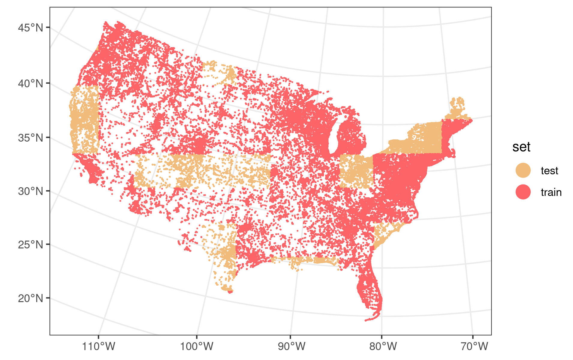
We used the eBird Basic Dataset (EBD) for our analysis. We focused on a single month, June 2019, and limited records to the United States of America. We also limited the species in the analysis to those found in the North American Breeding Bird Survey to facilitate comparisons with that dataset. Records outside of the mainland of the US were dropped. This resulted in 430 species with at least one observation. We further used the blockCV software package (Valavi et al. 2019) to split the dataset into four folds, of which we used three as a training set and the fourth as a spatially separated test set.
The basic unit of observation in the eBird dataset is the checklist. When an eBird user goes bird watching, they are asked to record the species they were able to identify. An important difference between eBird data and other citizen science datasets is that participants are asked whether they reported all species they were able to identify on their trip, or whether they included only a subset. They are strongly encouraged to report all species they were able to identify, and generally do so. We used only these complete records. The absence of this flag would complicate modelling, as it would be unclear whether an observer truly did not observe a species or chose not to report it.
In addition, eBird users are required to record a number of additional fields, depending on the protocol used. We subsetted the data to the three most common protocols:
- 1.
Traveling and Traveling – property specific (58.4% of checklists): Birds observed while travelling. Observers record the duration of their trip as well as the distance travelled.
- 2.
Stationary (40.0% of checklists): Birds seen while the observer stays at a certain location, recording the time spent.
- 3.
Area (0.4% of checklists): Birds seen while the observer systematically searches an area. Both the time spent searching and the area searched are recorded.
Each checklist record includes a single latitude and longitude entry. To ensure that these spatial coordinates were close to the location of the observations, we dropped checklists following the Traveling protocol with distances travelled greater than 3km, which resulted in roughly every third checklist in this protocol being dropped. For the same reason, we dropped checklists in the Area protocol with areas of over 9 km2 searched, of which there were only five.
The full dataset consisted of 323,299 checklists. After all filtering steps, a total of 246,149 checklists remained, of which 186,811 were in the training set, and the remaining 59,338 formed the test set. The locations of these checklists and the split into train and test sets chosen automatically by the blockCV package are shown in Figure 1.
Finally, we kept only species with at least five observations in the training set, resulting in a total of 426. Even after these processing steps, the dataset remained very large, at 186,811 observations of these 426 species. For comparison, the Swiss bird dataset used in Guillera-Arroita et al. 2019 consisted of 267 sites sampled 2-3 times with records for 158 species. If every site were sampled three times, this would result in 861 checklists. The full dataset considered here thus contains over 100 times as many observations of almost three times as many species, demonstrating the need for more scalable inference techniques.
2.4 Choice of covariates and sites
To fit the model described in subsection 2.1 to this dataset, we had to choose which environmental variables to include. Since climate is likely to strongly influence bird distribution, we included the worldclim climate variables (Hijmans et al. 2005) at a resolution of 10 minutes of a degree, which is roughly equivalent to about km2 in area.iviv iv This is the area spanned at the equator; at the latitudes in question, the equivalent area will be somewhat smaller. Among these, we removed highly correlated covariates as follows: going through each column in order, if a column of the design matrix had a sample correlation greater than 95% with a previous column, we dropped it from the analysis. This eliminated three of the nineteen covariates.
Occupancy detection models assume that the data consist of sites that are repeatedly visited. In surveys, sites are chosen and visited several times, while in eBird, checklist locations are not chosen systematically. To still be able to apply occupancy detection models, we broke the area of interest into sites. To do this, we used the environmental covariates to define a grid across the study area. The worldclim covariates are constant within cells of roughly km2 area, as described in the previous paragraph. Using these cells as the sites resulted in a total of 15,011 sites containing at least one checklist. Most cells (3,498) contained only a single checklist, but some contained hundreds, the most being 928.
At this point, we would like to point out a potential issue with our choice of data. The likelihood given in Equation 12 assumes that sites are independent conditional on the observation and environmental covariates. Although the assumption that checklists are collected independently from each other is likely to be reasonable, the occupancy of cells is likely to be spatially correlated, for example due to unmeasured covariates. Put simply, knowing that a species is present in one cell likely raises the probability of it being present in a neighbouring cell, even if the two locations have the same, or very similar, environmental covariates. The model presented here could be extended to also model spatial correlation, as was proposed for example in Johnson et al. 2013.
However, we choose not to pursue this route here, for the following reasons. Firstly, from a practical point of view, a spatial model would raise difficult computational challenges. Secondly, adding a spatial effect is also complicated by the problem of spatial confounding (Johnson et al. 2013; Hodges and Reich 2010) which, summarised briefly, says that adding a spatial effect can cause bias in the estimates of the coefficients of a regression model. To address spatial confounding, the spatially-correlated errors are often modified to explain only variation not explained by the environmental covariates. In such a modified model, the estimated environmental coefficients have the same posterior means, but larger variances (see Figure 1 in Johnson et al. 2013, for example). This means that the model presented should produce good posterior mean estimates of the environmental coefficients, even if their variance estimates are likely to be somewhat overconfident. In summary, we argue that while a spatial extension would be interesting and useful future work, the simpler approach presented here can still produce reasonable predictions.
In addition to the worldclim climate variables, we included land cover covariates derived from the National Land Cover Database in its 2016 iteration (Homer et al. 2012). We aggregated these as follows. Four of the covariates related to “developed” areas of varying intensity. We grouped these together into a single category. Three of the categories – “Unknown”, “Barren Land”, and “Perennial Ice/Snow” – were very rarely assigned, so we grouped them together into the category “Other”. Finally, we combined the two categories relating to wetlands into a single category.
We derived binary indicators of whether each cell contained a particular land cover. For example, the “has_open_water” covariate takes the value of 1 if the cell is partly classified as “Open Water”, and zero otherwise. We considered two alternative summaries: an indicator of the majority land cover for each cell, and the fraction of the cell occupied by each land cover type. We chose the binary indicator over the majority cover since it encodes more information. Compared to the fraction covered, we believe the indicator to be a more useful summary in a linear model. Our reasoning is that, taking a water bird as an example, the availability of any water is likely to drastically increase the probability that the cell is suitable, but the difference between, say, 20% or 40% of the cell being covered by water is unlikely to increase it much further.
A list of all environmental covariates used together with their means and standard deviations is given in Table 1 in the supplementary material. We further included the square of each worldclim covariate since the unimodal environmental responses implied by quadratic terms are more ecologically plausible than straight line fits. Some authors have argued that species response curves are skewed and thus quadratic terms are not sufficient (Austin 2007). The model could be extended to include spline terms or interactions to improve its fit, but for simplicity, we included only quadratic terms here. All in all, we used a total of 43 environmental covariates. All covariates apart from the indicators were standardised to have mean 0 and standard deviation 1 in the training data.
The observation covariates should be chosen to provide information about , the probability that a species is observed given that it is present. To do this, we included the (log-transformed) duration spent birding in minutes, as well as the protocol type (Stationary, Travelling, or Area). The detection probability is also likely to be affected by the time of day. To take this into account, we obtained the times of sunrise and sunset for each checklist and categorised the observation times into eight categories based on the time to sunrise and from sunset (please see section E of the supplementary material for a description of these categories).
We also expected the land cover to affect the probability of detection, for two reasons. Firstly, land cover can make it more difficult to detect species presence. For example, a densely wooded area may reduce visibility compared to an open grassy area. Secondly, checklists only cover part of the site: sites are around km2 in size, but checklists cover a route of 3 km at most. So, even though a site may be partly covered by forest, making it suitable for a forest-dwelling bird, the observations may not be made in that part of the cell. To take these factors into account, we used the NLCD dataset at a finer km2 resolution to determine the dominant land cover for each checklist and included this indicator as a covariate. We aggregated the land cover covariates more coarsely for the detection probability, to “Forest”, “Developed”, “Water”, and “Other”, since we expected these to affect detection probabilities the most. All together, this resulted in 13 covariates used to model the observation process.
2.5 Evaluation
Evaluating occupancy detection models is challenging, since no ground truth is available for the true presence and absence of species. We therefore evaluate the different approaches in two stages: first, by how well they are able to predict the observations in the spatially separated test set. This evaluation only assesses the model’s ability to predict joint detection and suitability, so its ability to separate the two is not evaluated. Our assumption is that better evaluation performance on the separated test set translates to improved estimates of occupancy, but we acknowledge that this is not necessarily so. For this reason, we also include a comparison of predicted suitability maps with expert range maps, which provides a qualitative evaluation of the model’s ability to separate the two processes.
To evaluate the utility of using more data, we fitted the proposed inference approaches – variational inference and MCMC – to different dataset sizes. We created smaller datasets from the full one by randomly selecting a sample of checklists from the training set, starting with 1,000 and doubling them until 32,000 checklists are reached. For variational inference, we also fitted 64,000 checklists, 100,000 checklists and, finally, the full training set of 186,811. As mentioned previously, the variational inference approach requires fixing a number of draws to estimate the objective, with large reducing bias but also requiring more memory. We used up to 4,000 checklists, for 8,000, for 16,000 up to 100,000, and for the full 186,811 checklists. Using should incur only a small amount of bias, so we did not explore using larger than this for the smaller number of checklists. For the larger datasets, we chose to be as large as possible given the available GPU memory.
We added two baseline models to compare against. First, we fitted the smallest dataset of 1,000 checklists with Stan (Stan Development Team 2020). We did this to ensure that the MCMC approach in numpyro worked as expected. Second, we fitted each species separately using maximum likelihood on the full dataset. We used only the full dataset since, unlike the Bayesian models which fall back to the prior in the absence of data, maximum likelihood inference requires a minimum number of observations to avoid singular estimates. Some species are observed very rarely, so only using the full dataset ensured that each species was observed at least once in the data.
As we increased the number of checklists, we faced two computational issues. When the dataset included more than 16,000 checklists, the MCMC approach in numpyro failed to converge using its default settings. We were able to address this by switching from single precision arithmetic to double precision. When using the variational inference approach, the largest checklist datasets required a large amount of GPU memory. For this reason, we used an NVIDIA P100 GPU with 16GB of memory for the variational inference approaches, while an NVIDIA GTX-2070 GPU with 8GB of memory was used for the MCMC approach.
To assess the quality of predictions, we use the area under the receiver operating characteristic curve (AUC) and mean log likelihood. AUC estimates the probability that a randomly chosen positive example will be ranked more highly than a randomly chosen negative example (Fielding and Bell 1997), making it easy to interpret. However, AUC only assesses the ability of the model to rank its predictions, not the calibration of the predicted probabilities. The log likelihood, our second metric, also assesses calibration, and it is maximised when the predicted probabilities are equal to the true probabilities, making it a proper scoring rule (Gneiting and Raftery 2007). We calculated each species’ mean log likelihood by computing the log probability assigned to the observed outcome in each checklist, and then computing its average. We refer the interested reader to Lawson et al. 2014 for a detailed discussion of the differences between AUC and log likelihood.
The metrics above evaluate how well the different methods are able to predict unseen, spatially separated data from the eBird dataset. As mentioned at the start of the section however, if model scores highly on these metrics, this does not necessarily mean that it is a good model of species distribution. Each data point in eBird is affected not only by the biological process of interest but also the observation process, and it cannot be used to evaluate either in isolation. To address this, we initially considered using the North American Breeding Bird Survey (BBS) (Pardieck et al. 2020), a high quality survey dataset, as ground truth. This dataset consists of routes, each of which is divided into fifty stops, spaced half a mile apart. At each stop, surveyors remain stationary for three minutes and record all bird species they were able to detect. Participants in the survey are highly skilled, but we believe that the BBS protocol is still likely to miss species that are actually present. For example, observations are made by roads, which may make it hard to observe certain kinds of species. They also tend to be made at a particular time of day (usually in the early morning) and the time spent per stop is short.
In view of these issues, we instead compared the models’ predictions against expert range maps from BirdLife International 2020. These expert maps also do not represent ground truth: they are based on subjective judgement, and they are generally not specified at a high level of detail. Still, good agreement with expert maps should indicate that a model is in line with established knowledge, which may build trust.
Our aim in using the expert maps was to answer two questions. First, how does the best MSOD model fitted to eBird compare to the same model fitted to high-quality BBS data; and second, how much is agreement improved when using an MSOD model compared to treating the data as presence/absence. To answer the first question, we fitted an MSOD model to BBS by treating the fifty stops made along each survey route as repeat visits to the same site. For the second, we fitted PA models to BBS and eBird. To do this for the BBS dataset, we treated a species as present if it was observed at least once on a route and absent otherwise. For eBird, we fitted a PA model by assuming that each checklist consisted of presence/absence data. To keep the PA models as similar to the MSOD models as possible, we used the same model for as in subsection 2.1, but treated as being directly observed.
To evaluate how well a model agrees with an expert map, we first predicted the probability of presence, , for each cell of the worldclim covariates in the study area. We then computed the square error between the predicted probability and the value in the expert map for each cell (either 1 or 0). We summarised the overall error by taking the mean of these square errors, which is also known as the Brier score.
3 Results
3.1 Evaluation results
Figure 2shows the evaluation results for different numbers of checklists. The top panel, comparing AUC, shows a clear increasing trend as the number of checklists increases. At 1,000 checklists, MCMC clearly outperforms VI, at around 83% AUC compared to about 80.1% for VI. This difference shrinks as the dataset size is increased, however, and at 32,000 checklists, VI’s AUC is essentially identical to MCMC’s. This suggests that, for prediction, the ability to capture posterior correlations becomes less important as the amount of data grows. Most of the improvement comes between the dataset sizes of 1,000 and 32,000, with AUC improving from 80% to 89.7% for VI. The very largest datasets improve AUC slightly further, with VI fitted to the entire dataset reaching 90.4% AUC. Maximum likelihood fitted to the entire dataset separately for each species achieves a lower AUC of around 88.7%. This gap suggests that modelling the observation process with a hierarchical model is able to improve predictions. Stan fitted to 1,000 checklists performs exactly as well as MCMC, suggesting that numpyro’s estimates are very similar to those made by Stan.
The middle panel, comparing log likelihood, shows a similar trend. There appears to be a slight downward trend as the number of checklists grows beyond 32,000 in VI, which may be because the number of fixed draws to approximate the objective is reduced to allow the model to be loaded in memory. The difference is very small, however, and unlikely to be important in practice. Maximum likelihood performs worse on log likelihood than on AUC: even hierarchical models fitted to a random sample of 2,000 checklists outperform maximum likelihood fitted to the entire dataset, indicating that calibration is substantially improved using the Bayesian multi-species models.
Finally, the bottom panel compares the runtime of the different approaches. The slowest of all approaches is Stan fitted to the 1,000 checklists. We note that while we attempted to write the Stan model efficiently, more could be done to improve its performance. Our purpose here is not to provide a benchmark comparing Stan and numpyro, but to use Stan as a trusted method to ensure numpyro is providing reliable estimates. numpyro’s runtime increased as the number of checklists grows, and fitting 32,000 checklists took around 18 hours. Variational inference was substantially faster, taking less than two hours to fit the largest dataset. Given the similar AUC and log-likelihood metrics but dramatically faster runtime, we believe VI to be the most compelling inference approach and analyse the detectability estimates of the model fitted to the full dataset using VI in the rest of the manuscript.
In the introduction, we suggested that multi-species occupancy detection models may be particularly useful to predict rarely-observed species due to their ability to borrow strength. To investigate this, we calculated the improvement in AUC for each species when using the MSOD model fitted using VI compared to maximum likelihood fitted separately to each species. Figure 3 shows these AUC improvements as a function of the number of observations for each species in the training dataset. The figure suggests that for the most common species with more than 1,000 presences or so, the single-species approach (using maximum likelihood) and the multi-species approaches generally achieve a similar AUC. For rarer species however, there appears to be a clear benefit to partially pooling the observation process: almost all species show a positive improvement in AUC, and some improve a considerable amount. Of those that show reduced AUC, almost all error bars overlap with zero, indicating that the proposed model almost always performs as well or better than maximum likelihood.

3.2 Detectability estimates
| Coefficient | Group mean | Group sd |
|---|---|---|
| Intercept | -1.83 | 0.86 |
| Protocol: Stationary | -0.43 | 0.38 |
| Protocol: Traveling | -0.03 | 0.00 |
| Daytime: Early morning | -0.16 | 0.27 |
| Daytime: Late morning | -0.32 | 0.27 |
| Daytime: Mid-day | -0.46 | 0.33 |
| Daytime: Early evening | -0.49 | 0.35 |
| Daytime: Late evening | -0.49 | 0.35 |
| Daytime: Dusk | -1.79 | 1.18 |
| Daytime: Night | -1.78 | 1.03 |
| Dominant Land Cover: Developed | -0.90 | 0.72 |
| Dominant Land Cover: Forest | -0.44 | 0.86 |
| Dominant Land Cover: Water | -0.47 | 0.60 |
| Log duration | 0.45 | 0.20 |
Table 1shows the group means and standard deviations inferred by the variational inference model fitted to all checklists in the training set. The reference classes for the categorical variables are “Area” for protocol, “dawn” for daytimes, and “Other” for land cover. The log duration is standardised so that a log duration of zero corresponds to about 22 minutes spent birding. The group intercept of suggests that a typical bird species has a probability of being detected when 22 minutes is spent following the Area protocol, but that a probability of or as high as would not be very surprising. In fact, the species with the lowest intercept is the Northern goshawk (Accipiter gentilis), whose intercept is , indicating that this species is very unlikely to be detected even if present. The American robin (Turdus migratorius) has the highest intercept at . The group mean for log duration is positive, indicating that in general, a longer time spent birding raises the chance of detection, as one might expect.
The means of -0.43 and -0.03 imply that compared to the Area protocol, bird species are somewhat less likely to be detected when following the Stationary protocol, and roughly as likely when following the Traveling protocol. The group standard deviation of 0.38 suggests that there is variability among the Stationary coefficients by species, and indeed they range from -1.37 for Bell’s vireo (Vireo bellii) to 1.14 for the Ruby-throated hummingbird (Archilochus colubris). It is likely that the stationary protocol is often followed by observers in their back yards, where hummingbirds are often attracted to feeders, which may explain this high coefficient. By contrast, the group standard deviation for the Traveling protocol is zero, indicating that the variational inference procedure estimates no difference among birds here compared to the Area protocol.
All daytime group means are smaller than zero, suggesting that most bird species are most easily detected at dawn, the reference class, which is consistent with common knowledge. Birds are typically considerably less likely to be detected at dusk and night, but the group standard deviations of 1.18 and 1.03, respectively, indicate that there is considerable variation by species. Figure 4 investigates this in more depth. Species above the dashed line are more likely to be detected at night, while those below it (the majority) are more likely to be detected at dawn. For some species, the difference is dramatic: the Eastern Whip-poor-will (Antrostomus vociferus), for instance, is estimated to be very likely to be detected at night (61.3%) but quite unlikely to be detected at dawn (5.2%). The other species more likely to be detected at night are generally other noctural species such as owls and other nightjars, which appears reasonable.
All three land cover categories are estimated to decrease the probability of detecting most birds. The largest amount of variability is estimated to be among the forest cover class, at 0.86. Abert’s Towhee (Melozone aberti) is estimated to be much less likely to be detected in forests (-3.88), while the Varied Thrush (Ixoreus naevius) is much more likely to be detected there (+1.88).

3.3 Expert map evaluation
Figure 5shows the mean Brier score across species for each combination of model (MSOD and PA) and dataset (eBird and BBS). A lower Brier score indicates better agreement, on average, with the expert maps from BirdLife International 2020. The figure shows that there is a large improvement in agreement when using MSOD models on eBird compared to PA, emphasising the importance of accounting for the observation process. The MSOD model fitted to eBird has the lowest Brier score on average, but there is overlap in the standard errors with MSOD fitted to BBS. Comparing the Brier scores between these approaches, MSOD fitted to eBird had a lower error for 238 of 357 birds, or 66.7%. A sign test suggested that this advantage is very unlikely to be due to chance (). Figure S2 in the supplementary material investigates the differences between these approaches further by comparing the Brier scores for these two approaches. Most scores are similar, but MSOD on eBird may agree slightly better when predicting water birds. Fitting the MSOD model slightly improves agreement on BBS compared to PA, but the change is not as dramatic as for the eBird dataset. We also provide an interactive web applicationvv v Accessible here: https://martiningram.shinyapps.io/range_map_comparisons/ where range maps predicted by the four approaches can be compared for species of interest. Overall, the results suggest that an MSOD model fitted to eBird data agrees with expert maps at least as well as the same model fitted to the high-quality survey data.

When comparing to BBS, it became apparent that the eBird data may be particularly useful for predicting the distributions of rare species. In the comparison above, we included only species that were observed at least eight times in the BBS data, as species with fewer observations were unlikely to be well estimated. Of the species fitted here, 47 were observed this rarely. About 80.8% of these are observed at least 20 times in the eBird dataset, and 55.3% are observed more than 100 times, increasing the number of species for which predictions could be made. Figure 6 shows one such species: the Northwestern Crow (Corvus caurinus). This species had zero observations in the BBS training set and a prediction was thus impossible. By contrast, eBird contained 213 observations of Corvus caurinus in the training set, and the suitability map predicted in Figure 6 agrees well with the expert map.


We note that the predicted map in Figure 6 shows the posterior mean. The posterior mean is a reasonable point estimate as it minimises the expected square error (see e.g. (Berger 1985, p.161)), but it does not show the uncertainty in the posterior. We discuss how to obtain and visualise the uncertainty in the model’s predictions in section H of the supplementary material.
4 Discussion and conclusions
The focus of this paper was to develop methods to scale multi-species occupancy detection models to large datasets. We believe them to be a compelling model for citizen science data, making the most of the wealth of data collected while accounting for the heterogeneity in the observation process.
The ability to partially pool the coefficients in the observation process sets this work apart from previous work applying occupancy detection models to citizen science data. For example, Johnston et al. 2019 fitted a single-species occupancy detection model to a single bird species using eBird data. In this work, we have shown that partial pooling can improve model predictions, both in AUC and log likelihood.
Another approach taken in Johnston et al. 2019 was to model the encounter rate using random forests. Such models are able to model complicated environmental responses, which may provide a better fit to the observed data. However, this added flexibility comes at the cost of interpretability: the high-dimensional interactions and non-linear functions fitted by random forests can be hard to understand. Perhaps more importantly, unlike occupancy detection models, random forests cannot estimate detection and occupancy probabilities separately, further complicating interpretation. A more compelling alternative could be to retain the occupancy detection modelling framework but use either generalised additive (Hastie and Tibshirani 1986) or Gaussian process models (Ingram et al. 2020) to allow for more complex environmental responses.
A key result of the paper is that, when evaluated against expert maps, the model fitted to citizen science data performs at least as well as the same model fitted to the high quality BBS dataset. As we have pointed out, compared to survey data, citizen science data has the advantage of being more abundant, allowing predictions to be made for rare species like the Northwestern crow (Corvus caurinus). In addition, while the BBS is only performed once a year, eBird data is collected throughout, and the model presented could be fitted to different time periods to investigate how distributions change over the course of a year, or over time.
We see a number of ways to further refine the proposed model. The detection probabilities could be made observer-specific, perhaps using an estimate of observer skill such as that derived by Kelling et al. 2015. The possibility of false positives could be taken into account, perhaps using the methodology of Yu et al. 2014 to identify species most at risk of being confused. To estimate changes in occupancy over time, a dynamic version of the proposed model could be developed (Royle and Kéry 2007). The prior means could also be refined using species-specific information: for example, a species indicator of whether it is nocturnal or not could be used to set a prior expectation for the daytime coefficients.
As discussed previously, the model presented in this paper is non-spatial and treats presences in each cell as independent conditional on the environmental covariates. We have argued that this is a reasonable approximation, but we believe that extending the model to account for spatial autocorrelation would be worthwhile and should improve posterior variance estimates. A second useful spatial extension could be to allow the environmental coefficients to vary throughout each species’ range (Osborne et al. 2007). This could improve the model’s predictions, as the study region is large, and species’ environmental responses may differ across their range.
From the point of view of ecological research, we are excited about the possible applications of our approach. The ability to make estimates for species too rare in the BBS could be used to investigate their range shifts over time. To this end, the model could be fitted to data from previous years, and the range estimates could be compared. Similarly, because eBird is collected each month, changes in phenology, such as species migration patterns, could be assessed. While maps of species migration are already being produced with eBird data (see Sullivan et al. 2009, for example), our estimates corrected for observer bias may be preferable, especially when data are sparse. We also note that apart from the set of covariates chosen, our approach is general and not tied to the eBird dataset. It could thus be applied also to other citizen science datasets, and other species.
Finally, we would like to emphasise that the reason occupancy detection models can be fitted to eBird data is the existence of the flag indicating that all species that were observed were reported. Without this flag, eBird data would be presence-only data, and at best we could only estimate relative suitability (see Guillera-Arroita et al. 2015, for example). With the flag, as we have shown, reasonable predictions can be made which we argued can even compete with those based on systematic surveys. We believe that this has strong implications for the design of citizen science protocols: citizen scientists should be asked to report not only which species they observed, but also which species they were looking for but did not observe.
Acknowledgements
We would like to thank the Associate Editor and the two anonymous reviewers for their valuable feedback. We would also like to thank Alison Johnston for her helpful comments and suggestions on an early version of the manuscript.
This research was undertaken using the LIEF HPC-GPGPU Facility hosted at the University of Melbourne. This Facility was established with the assistance of LIEF Grant LE170100200. MI was partially supported by a Melbourne Research Scholarship. NG was supported by an ARC DECRA fellowship (DE180100635).
Authors’ contributions
All authors conceived the ideas and methodology. MI implemented the analysis. MI led writing the manuscript but all authors contributed significantly throughout and gave final approval before submission.
Data accessibility
- •
Scripts to fit the models discussed in this paper are available in a GitHub repository for python https://github.com/martiningram/occu_py and R (recommended) https://github.com/martiningram/roccupy.
- •
The eBird dataset used in this paper is the eBird Basic Dataset (EBD), which is freely available at https://ebird.org/data/download (Sullivan et al. 2009). The code we used to process this data is available at https://github.com/martiningram/ebird-prep.
- •
The Breeding Bird Survey (BBS) dataset used in this paper is freely available from ScienceBase: https://www.sciencebase.gov/catalog/item/5ea04e9a82cefae35a129d65.
References
- Altwegg and Nichols (2019) Res Altwegg and James D. Nichols. Occupancy models for citizen-science data. Methods in Ecology and Evolution, 10(1):8–21, 2019. https://doi.org/10.1111/2041-210X.13090. URL https://besjournals.onlinelibrary.wiley.com/doi/abs/10.1111/2041-210X.13090.
- Austin (2007) Mike Austin. Species distribution models and ecological theory: A critical assessment and some possible new approaches. Ecological Modelling, 200(1):1 – 19, 2007. ISSN 0304-3800. https://doi.org/10.1016/j.ecolmodel.2006.07.005.
- Berger (1985) James O Berger. Statistical decision theory and Bayesian analysis; 2nd ed. Springer series in statistics. Springer, New York, 1985. 10.1007/978-1-4757-4286-2. URL https://cds.cern.ch/record/1327974.
- BirdLife International (2020) BirdLife International. Bird species distribution maps of the world. Version 2020.1. 2020. URL http://datazone.birdlife.org/species/requestdis.
- Bradbury et al. (2018) James Bradbury, Roy Frostig, Peter Hawkins, Matthew James Johnson, Chris Leary, Dougal Maclaurin, George Necula, Adam Paszke, Jake VanderPlas, Skye Wanderman-Milne, and Qiao Zhang. JAX: composable transformations of Python+NumPy programs, 2018. URL http://github.com/google/jax.
- Dickinson et al. (2010) Janis L. Dickinson, Benjamin Zuckerberg, and David N. Bonter. Citizen science as an ecological research tool: Challenges and benefits. Annual Review of Ecology, Evolution, and Systematics, 41(1):149–172, 2010. 10.1146/annurev-ecolsys-102209-144636. URL https://doi.org/10.1146/annurev-ecolsys-102209-144636.
- Fielding and Bell (1997) Alan H Fielding and John F Bell. A review of methods for the assessment of prediction errors in conservation presence/absence models. Environmental Conservation, 24(1):38–49, 1997.
- Fiske and Chandler (2011) Ian Fiske and Richard Chandler. unmarked: An R Package for Fitting Hierarchical Models of Wildlife Occurrence and Abundance. Journal of Statistical Software, 43(10):1–23, 2011. URL http://www.jstatsoft.org/v43/i10/.
- Giordano et al. (2018) Ryan Giordano, Tamara Broderick, and Michael I. Jordan. Covariances, Robustness, and Variational Bayes. Journal of Machine Learning Research, 19(51):1–49, 2018. URL http://jmlr.org/papers/v19/17-670.html.
- Gneiting and Raftery (2007) Tilmann Gneiting and Adrian E Raftery. Strictly Proper Scoring Rules, Prediction, and Estimation. Journal of the American Statistical Association, 102(477):359–378, 2007. 10.1198/016214506000001437. URL https://doi.org/10.1198/016214506000001437.
- Golding (2019) Nick Golding. greta: simple and scalable statistical modelling in R. Journal of Open Source Software, 4(40):1601, 2019. 10.21105/joss.01601. URL https://doi.org/10.21105/joss.01601.
- Guillera-Arroita (2017) Gurutzeta Guillera-Arroita. Modelling of species distributions, range dynamics and communities under imperfect detection: advances, challenges and opportunities. Ecography, 40(2):281–295, 2017. https://doi.org/10.1111/ecog.02445. URL https://onlinelibrary.wiley.com/doi/abs/10.1111/ecog.02445.
- Guillera-Arroita et al. (2015) Gurutzeta Guillera-Arroita, José J. Lahoz-Monfort, Jane Elith, Ascelin Gordon, Heini Kujala, Pia E. Lentini, Michael A. McCarthy, Reid Tingley, and Brendan A. Wintle. Is my species distribution model fit for purpose? Matching data and models to applications. Global Ecology and Biogeography, 24(3):276–292, 2015. https://doi.org/10.1111/geb.12268. URL https://onlinelibrary.wiley.com/doi/abs/10.1111/geb.12268.
- Guillera-Arroita et al. (2019) Gurutzeta Guillera-Arroita, Marc Kéry, and José J. Lahoz-Monfort. Inferring species richness using multispecies occupancy modeling: Estimation performance and interpretation. Ecology and Evolution, 9(2):780–792, 2019. https://doi.org/10.1002/ece3.4821. URL https://onlinelibrary.wiley.com/doi/abs/10.1002/ece3.4821.
- Harris (2015) David J. Harris. Generating realistic assemblages with a joint species distribution model. Methods in Ecology and Evolution, 6(4):465–473, 2015. https://doi.org/10.1111/2041-210X.12332. URL https://besjournals.onlinelibrary.wiley.com/doi/abs/10.1111/2041-210X.12332.
- Hastie and Tibshirani (1986) Trevor Hastie and Robert Tibshirani. Generalized Additive Models. Statistical Science, 1(3):297 – 310, 1986. 10.1214/ss/1177013604. URL https://doi.org/10.1214/ss/1177013604.
- Hijmans et al. (2005) Robert J. Hijmans, Susan E. Cameron, Juan L. Parra, Peter G. Jones, and Andy Jarvis. Very high resolution interpolated climate surfaces for global land areas. International Journal of Climatology, 25(15):1965–1978, 2005. 10.1002/joc.1276.
- Hodges and Reich (2010) James S. Hodges and Brian J. Reich. Adding spatially-correlated errors can mess up the fixed effect you love. The American Statistician, 64(4):325–334, 2010. 10.1198/tast.2010.10052. URL https://doi.org/10.1198/tast.2010.10052.
- Hoffman and Gelman (2014) Matthew D. Hoffman and Andrew Gelman. The No-U-Turn Sampler: Adaptively Setting Path Lengths in Hamiltonian Monte Carlo. Journal of Machine Learning Research, 15(47):1593–1623, 2014. URL http://jmlr.org/papers/v15/hoffman14a.html.
- Homer et al. (2012) Collin H Homer, Joyce A Fry, and Christopher A Barnes. The National Land Cover Database. US Geological Survey Fact Sheet, 3020(4):1–4, 2012.
- Ingram et al. (2020) Martin Ingram, Damjan Vukcevic, and Nick Golding. Multi-output Gaussian processes for species distribution modelling. Methods in Ecology and Evolution, 11(12):1587–1598, 2020. https://doi.org/10.1111/2041-210X.13496. URL https://besjournals.onlinelibrary.wiley.com/doi/abs/10.1111/2041-210X.13496.
- Johnson et al. (2013) Devin S. Johnson, Paul B. Conn, Mevin B. Hooten, Justina C. Ray, and Bruce A. Pond. Spatial occupancy models for large data sets. Ecology, 94(4):801–808, 2013. https://doi.org/10.1890/12-0564.1. URL https://esajournals.onlinelibrary.wiley.com/doi/abs/10.1890/12-0564.1.
- Johnston et al. (2019) A Johnston, WM Hochachka, ME Strimas-Mackey, V Ruiz Gutierrez, OJ Robinson, ET Miller, T Auer, ST Kelling, and D Fink. Best practices for making reliable inferences from citizen science data: case study using eBird to estimate species distributions. bioRxiv, 2019. 10.1101/574392. URL https://www.biorxiv.org/content/early/2019/03/13/574392.
- Kelling et al. (2015) Steve Kelling, Alison Johnston, Wesley M. Hochachka, Marshall Iliff, Daniel Fink, Jeff Gerbracht, Carl Lagoze, Frank A. La Sorte, Travis Moore, Andrea Wiggins, Weng-Keen Wong, Chris Wood, and Jun Yu. Can Observation Skills of Citizen Scientists Be Estimated Using Species Accumulation Curves? PLOS ONE, 10(10):1–20, 10 2015. 10.1371/journal.pone.0139600. URL https://doi.org/10.1371/journal.pone.0139600.
- Kery and Royle (2009) M. Kery and J. Andrew Royle. Inference about species richness and community structure using species-specific occupancy models in the National Swiss Breeding Bird Survey MUB, pages 639–656. Modeling demographic processes in marked populations. Springer, New York and London, 2009. URL http://pubs.er.usgs.gov/publication/5211455.
- Kucukelbir et al. (2017) Alp Kucukelbir, Dustin Tran, Rajesh Ranganath, Andrew Gelman, and David M. Blei. Automatic Differentiation Variational Inference. Journal of Machine Learning Research, 18(14):1–45, 2017. URL http://jmlr.org/papers/v18/16-107.html.
- Lawson et al. (2014) Callum R Lawson, Jenny A Hodgson, Robert J Wilson, and Shane A Richards. Prevalence, thresholds and the performance of presence–absence models. Methods in Ecology and Evolution, 5(1):54–64, 2014.
- Lunn et al. (2000) David J. Lunn, Andrew Thomas, Nicky Best, and David Spiegelhalter. WinBUGS - A Bayesian modelling framework: Concepts, structure, and extensibility. Statistics and Computing, 10(4):325–337, Oct 2000. ISSN 1573-1375. 10.1023/A:1008929526011. URL https://doi.org/10.1023/A:1008929526011.
- MacKenzie et al. (2002) Darryl I. MacKenzie, James D. Nichols, Gideon B. Lachman, Sam Droege, J. Andrew Royle, and Catherine A. Langtimm. Estimating site occupancy rates when detection probabilities are less than one. Ecology, 83(8):2248–2255, 2002. https://doi.org/10.1890/0012-9658(2002)083[2248:ESORWD]2.0.CO;2. URL https://esajournals.onlinelibrary.wiley.com/doi/abs/10.1890/0012-9658%282002%29083%5B2248%3AESORWD%5D2.0.CO%3B2.
- Monnahan et al. (2017) Cole C. Monnahan, James T. Thorson, and Trevor A. Branch. Faster estimation of Bayesian models in ecology using Hamiltonian Monte Carlo. Methods in Ecology and Evolution, 8(3):339–348, 2017. https://doi.org/10.1111/2041-210X.12681. URL https://besjournals.onlinelibrary.wiley.com/doi/abs/10.1111/2041-210X.12681.
- Osborne et al. (2007) Patrick E. Osborne, Giles M. Foody, and Susana Suárez-Seoane. Non-stationarity and local approaches to modelling the distributions of wildlife. Diversity and Distributions, 13(3):313–323, 2007. ISSN 13669516, 14724642. URL http://www.jstor.org/stable/4539924.
- Pardieck et al. (2020) K.L. Pardieck, D.J. Ziolkowski Jr, M. Lutmerding, V.I. Aponte, and M-A.R. Hudson. North American Breeding Bird Survey Dataset 1966-2019: U.S. Geological Survey data release. US Geological Survey, Patuxent Wildlife Research Center, 2020. 10.5066/P9J6QUF6.
- Phan et al. (2019) Du Phan, Neeraj Pradhan, and Martin Jankowiak. Composable Effects for Flexible and Accelerated Probabilistic Programming in NumPyro. arXiv preprint arXiv:1912.11554, 2019.
- Royle and Kéry (2007) J. Andrew Royle and Marc Kéry. A Bayesian state-space formulation of dynamic occupancy models. Ecology, 88(7):1813–1823, 2007. https://doi.org/10.1890/06-0669.1. URL https://esajournals.onlinelibrary.wiley.com/doi/abs/10.1890/06-0669.1.
- Royle et al. (2007) J. Andrew Royle, Robert M Dorazio, and William A Link. Analysis of Multinomial Models With Unknown Index Using Data Augmentation. Journal of Computational and Graphical Statistics, 16(1):67–85, 2007. 10.1198/106186007X181425. URL https://doi.org/10.1198/106186007X181425.
- Stan Development Team (2020) Stan Development Team. RStan: the R interface to Stan, 2020. URL http://mc-stan.org/. R package version 2.21.2.
- Sullivan et al. (2009) Brian L. Sullivan, Christopher L. Wood, Marshall J. Iliff, Rick E. Bonney, Daniel Fink, and Steve Kelling. eBird: A citizen-based bird observation network in the biological sciences. Biological Conservation, 142(10):2282–2292, 2009. ISSN 0006-3207. https://doi.org/10.1016/j.biocon.2009.05.006. URL https://www.sciencedirect.com/science/article/pii/S000632070900216X.
- Valavi et al. (2019) Roozbeh Valavi, Jane Elith, José J Lahoz-Monfort, and Gurutzeta Guillera-Arroita. blockCV: An R package for generating spatially or environmentally separated folds for k-fold cross-validation of species distribution models. Methods in Ecology and Evolution, 10(2):225–232, 2019.
- Yu et al. (2014) Jun Yu, Rebecca Hutchinson, and Weng-Keen Wong. A Latent Variable Model for Discovering Bird Species Commonly Misidentified by Citizen Scientists. Proceedings of the AAAI Conference on Artificial Intelligence, 28(1), Jun. 2014. URL https://ojs.aaai.org/index.php/AAAI/article/view/8763.