Modeling, robust control synthesis and worst-case analysis for an on-orbit servicing mission with large flexible spacecraftJournal: Aerospace Science and Technology
Abstract
This paper outlines a complete methodology for modeling an on-orbit servicing mission scenario and designing a feedback control system for the attitude dynamics that is guaranteed to robustly meet pointing requirements, despite model uncertainties as well as large inertia and flexibility changes throughout the mission scenario. A model of the uncertain plant was derived, which fully captures the dynamics and couplings between all subsystems as well as the decoupled/coupled configurations of the chaser/target system in a single linear fractional representation (LFR). In addition, a new approach is proposed to model and analyze a closed-loop kinematic chain formed by the chaser and the target spacecraft through the chaser’s robotic arm, which uses two local spring-damper systems with uncertain damping and stiffness. This approach offers the possibility to model the dynamical behaviour of a docking mechanism with dynamic stiffness and damping. The controller was designed by taking into account all the interactions between subsystems and uncertainties as well as the time-varying and coupled flexible dynamics. Lastly, the robust stability and worst-case performances were assessed by means of a structured singular value analysis.
Keywords:
On-orbit servicing , Multibody modeling , Flexible structures , Robust control , Worst-case analysis1 Introduction
1.1 Background and motivation
On the one hand, the autonomous assembly of large structures in space is a key challenge for missions possessing structures to be self-deployed as a single piece, like PULSAR, which is able to overcome the size restrictions of current launchers [1, 2, 3]. On the other hand, there are also many ongoing on-orbit servicing (OOS) projects, which fall into three main categories: observation, motion and manipulation [4]. Both ESA’s Clean Space initiative and NASA’s Orbital Debris Program Office are mainly focused on de-orbiting satellites, while investigating the capture of a satellite by means of space robotics [5]. However, the use of robotics can also be a solution for different types of OOS missions such as maintenance, repair, refuel, upgrade and docked inspection of a satellite, which come under the manipulation category. NGIS’ MEV-1 [6] and EROSS [7, 8, 9] are some of the examples.
Over the years, a wide variety of studies has been conducted on the topic of spacecraft on-orbit rendezvous and assembly with disturbance rejection [10, 11, 12, 13, 14, 15]. However, most of these studies neglect flexibility and study the system as a rigid mass. Moreover, some papers consider the presence of uncertainties when doing control design [16]. When it comes to study the docking with another satellite on-orbit, some approaches acknowledge the capture mechanism as a simple basket [15], while others consider the usage of a robotic arm for this purpose [17, 18, 19, 20]. Nevertheless, these studies do not analyze in depth the change in mechanical properties due to the robotic arm movement while being docked to a target spacecraft with flexible appendages and considerable mass/inertial properties. Several docking mechanisms such as HOTDOCK [2] or ASSIST [21] are also being developed in order to make OOS missions possible. The contact dynamics model of ASSIST is built in a simulator [21] by considering the forces and torques caused by physical contact between the chaser and target spacecraft. However, no symbolic linear model is obtained in order to consider this effect when designing a controller.
From an AOCS/GNC point of view, this type of complex missions is particularly challenging due to the time-varying & coupled flexible dynamics. Consequently, the success of these projects is constrained by the ability to have an accurate model of the system and analysis tools which allow to predict the worst-case scenarios during preliminary design phases.
In this context, this paper aims at proposing an end-to-end structure/control co-design activity for an on-orbit servicing mission scenario. The ambition is to fill an important gap in the literature by taking into account flexibility and system uncertainty in the design of a robust controller to be used in an orbital servicing operation. In fact, this kind of scenario will be more and more frequent in the near future of space missions, where on-orbit operations of large and flexible structures will be put in place. In this context, a full modeling of multibody complex structures can help predicting in a very early phase the worst-case scenarios and push the control system to its limits of performance. Moreover, the availability of a model valid for any possible configuration simplifies the synthesis of the controller, which does not have to switch from one control mode to another. The transition between different control phases is in fact a critical aspect of the control design, that often implies intermediate tranquilization time windows.
The goal is then to establish a methodology for performing robust control system design and worst-case analysis for an on-orbit servicing scenario involving the interaction between two flexible vehicles. A Linear Parameter-Varying (LPV) model of two flexible multibody systems was firstly obtained. This model is fully parameterized according to the system’s geometrical configuration and was built using the Two-Input Two-Output Ports (TITOP) approach [22, 23, 24, 25, 26, 27], which offers the possibility to model complex multibody mechanical systems, while keeping the uncertain nature of the plant and condensing all the possible mechanical configurations in a single low order LFR. This model is then ready for robust control synthesis as well as robust stability and performance assessment [28]. All the models derived with the TITOP approach have been systematically implemented in the last release of the Satellite Dynamics Toolbox (SDT) [29], which allows the user to easily build the model of a flexible spacecraft with several appendages by assembling elemental Simulink customized blocks.
The chosen scenario is a system composed of two different spacecraft, a chaser and a target, both with large flexible solar arrays. The target, also called client satellite, is considered collaborative and prepared as it should be designed with specific features to facilitate the rendezvous and capture. First, the chaser performs a rendezvous with the target. Subsequently, the collaborative target is grasped by means of a robotic arm. Finally, the target vehicle is rigidly attached to one of the docking ports on the chaser to free up the robotic manipulator. This type of mission could be used to perform some maintenance on the target spacecraft, but also to use this target as a mission extension pod. It should be noted that this is just a scenario chosen to demonstrate the capabilities of the proposed approach. A multitude of other mission concepts such as on-orbit assembly or refueling could be explored using the same toolset.
1.2 Contributions and paper organization
The paper introduces the following key contributions:
- 1.
the development of a complete model fully capturing the dynamics and interactions between all subsystems of an OOS scenario: robotic arm, flexible appendages, decoupled/coupled configurations in a single LFR. This model includes the various interactions and uncertainty effects in a very compact representation. The fact that this model is minimal is critical to allow the usage of modern controller synthesis and analysis tools, which call for reduced numerical complexity.
- 2.
a new approach to the modeling of a closed-loop kinematic chain, which uses an uncertain local damping and stiffness in order to model the dynamical behaviour of a docking mechanism.
- 3.
a thorough controller synthesis and analysis procedure for the design of a static and structured attitude controller, taking into account all the various interactions and couplings which exist between different subsystems.
This paper is organized into three parts: system modeling, controller design and stability and performance analysis. In the first part (section 2), a symbolic linear model for control synthesis is obtained using SDT. The result is an LFR, minimal in terms of parameter occurrences. The proposed modeling design is verified using a non-linear physics simulator built with the Simscape multibody toolset from Mathworks. In the second part of the paper (section 3), the SDT model is used to design and optimize a controller capable of complying with the performance requirements which are imposed as constraints on the feedback loop. Finally, the third part (section 4) details the rigorous analysis procedure that was used to obtain robust performance and robust stability certificates.
2 Multibody Modeling Approach
2.1 The TITOP approach
The link connected to the parent substructure at the point and to the child substructure at point is depicted in Fig. 1a. The double-port or TITOP model is a linear dynamic model between 12 inputs:
- 1.
the six components in of the wrench applied by the substructure to the link at point stands for the three-component force vector applied at point , and stands for the three-component torque vector applied at point .
- 2.
the six components in of the acceleration twist of point : stands for the three-component linear acceleration vector at point , and stands for the three-component angular acceleration vector at point .
and 12 outputs:
- 1.
the six components in of the acceleration twist .
- 2.
the six components in of the wrench that is applied by the link to the substructure at point .
and can be represented by the block-diagram depicted in Fig. 1b. The way to obtain such a TITOP model will be detailed later.

2.2 SDT and Simscape modeling
For the on-orbit servicing mission scenario being studied in this paper, two different spacecraft are considered, the chaser and the target, which can be observed in Fig. 2.

The chaser spacecraft is composed of a rigid hub, two symmetric flexible solar arrays and one robotic arm. The target vehicle consists of a rigid hub and two flexible solar arrays. Initially, the chaser’s robotic arm is stretched near the bottom surface of the vehicle. While the chaser performs a rendezvous with the target, the arm starts its motion in order to dock to the other spacecraft. After seizing the vehicle, the robotic manipulator attaches it to the chaser’s rigid body by means of another docking mechanism. Finally, the chaser’s solar panels start rotating with the objective of optimizing the power being provided to the coupled system. For a better understanding of the mission scenario being studied, Fig. 3 depicts six different representations of the decoupled and coupled systems during the whole final rendezvous phase.

Let us now introduce in Table 1 the block-diagram representations based on the dynamic models of the several elements that will be used to build the full model of the system. A detailed analysis of each model will be provided later in the following sections of this paper. In this table, describes the rigid kinematic model between the degrees of freedom (DOF) of point and the DOF of point projected in frame . It is given by:
| (1) |
where represents the skew-symmetric matrix that results from the vector and is the coordinate vector of projected in frame . Furthemore, the transformation matrix between frames and is equal to:
| (2) |
where is a Direct Cosine Matrix (DCM) that transforms to (i.e., the matrix of components of unitary vectors in ). is a six-by-six matrix due to the fact that six DOF are being considered (three translations and three rotations).
2.2.1 Rigid hub model
A general rigid hub with center of mass can be modeled using the SDT’s block Multi-port rigid body, which computes the inverse linearized dynamic model of a rigid body at n given points, as explained in the SDT’s user guide [29]. Considering that the rigid body is submitted to external forces/moments and to forces/moments due to the interactions with an appendage connected at point , the linearized Newton/Euler equations read:
| (3) |
where is the static direct dynamic model of at the body’s center of mass and is the linear acceleration vector of at . Furthermore, is the mass of and represents the inertia tensor of written in the body frame of the rigid hub.
Looking now at the case of the OOS mission scenario being studied, the rotating body frames of the rigid hubs of the chaser and target spacecraft are represented in Fig. 2 (for the sake of simplicity, the x-axes are displayed in solid red lines, the y-axes in dashed green lines and the z-axes in dash-dotted blue lines). The body reference frame of the chaser’s rigid hub is given by , where is the center of mass and reference point of the main body. The same applies to the target’s rigid hub , with .
Since the chaser’s rigid hub is considered to be the system’s main body, is denoted as the angular velocity vector of the body frame with respect to the inertial frame , expressed in . Initially, when the chaser spacecraft is decoupled from the target, is connected to two solar arrays at points and as well as to one robotic arm at point . However, point of will eventually dock to point of , as can be observed in illustrations \normalsize5⃝ and \normalsize6⃝ in Fig. 3. For that reason, this port also needs to be considered. Furthermore, it is also considered that external forces and torques are acting on at point . is finally modeled using the compact representation \normalsizeA⃝ shown in Table 1. The inverse linearized dynamic model of defined in is then equal to .
Connection between rigid hubs: The frame transformation block-diagram based on the compact representation \normalsizeE⃝ in Table 1 is used to connect to at point .
Similarly to the chaser’s rigid hub, is connected to two solar arrays at points and . However, two docking phases will occur. Firstly, the end effector of the robotic arm located at point will dock to point of the target’s rigid hub , as can be seen in illustrations \normalsize5⃝ and \normalsize6⃝, with point being displayed in Fig. 4a. Secondly, port of will also dock to port of , as referred before.
Mechanical uncertainty : One of the objectives of this paper is to demonstrate how to design a controller in the presence of significant model uncertainty. For that reason, relative uncertainty is taken into account on the mass and moments of inertia of , since the robust stability and performance of the coupled system need to be ensured even when the mechanical characteristics of the target’s rigid hub are not perfectly known. As an example, let us now consider the mass of the target’s rigid body as uncertain:
| (4) |
where is the body’s nominal mass, is used to set the maximum percent of variation for the body’s mass and is a normalized real uncertainty. In the case of the mass, appears three times in a minimal LFR of a rigid body [29]. Therefore, the uncertainty block regarding the mass of is equal to . Similarly, relative uncertainty is also considered on the inertial properties of . However, only the diagonal moments of inertia were assumed to be uncertain while the off-diagonal terms are kept at their nominal values. For the moments of inertia of the target’s rigid hub , and , the normalized real uncertainties , and have just one occurrence in the same minimal LFR [29], where and are used to set the maximum percent of variation for , just like in Eq. (4). Therefore, the mechanical uncertainty block of the target’s rigid body can be written as . The dynamic model of will although be defined later in this paper.
In Simscape, the Inertia block is used to model a rigid body, which assumes the mass to be distributed in space, allowing the rigid hubs to have non-zero moments of inertia, products of inertia and center-of-mass coordinates.
2.2.2 Dynamic model of a cantilevered solar array
A general flexible solar array connected to a parent body at point can be modeled in SDT using the block One-port flexible body, as explained in [29]. The effective mass model of the solar array relates the six DOF acceleration vector of point and the six DOF forces/moments vector applied by the parent body to the appendage at point :
| (5) |
where:
- 1.
is the linear acceleration vector of at .
- 2.
and are the natural frequency, the damping ratio and the 6 DOF participation factor vector of the -th flexible mode of the appendage .
- 3.
is the matrix of modal participation factors of the flexible modes of the appendage at point .
- 4.
is the 6-by-6 residual mass/inertia of the appendage rigidly cantilevered to the parent body at point .
- 5.
is the 6-by-6 effective mass/inertia matrix of the -th flexible mode of the appendage.
MATLAB’s Partial Differential Equation (PDE) Toolbox is used to perform finite element analysis and extract all these structural dynamics parameters based on the 3D model of each solar array, its material properties and the boundary conditions. All the reference frames of the solar arrays are depicted in Fig. 2, where points represent the connection and reference points of the four flexible appendages. In addition, points are the solar arrays’ centers of mass. The effective mass models of the solar arrays are based on the compact representation \normalsizeC⃝ shown in Table 1 and equal to , with being described in Eq. (5).
In Simscape, the same process is achieved by means of the Reduced Order Flexible Solid block, which takes into account three mass, stiffness and damping matrices which are obtained by applying the Craig-Bampton order reduction method while considering the solar arrays to be cantilevered at points .
Modal uncertainty : Changes in structural parameters can provoke variations in the natural frequency of some flexible modes. Since the final goal is to design a controller where the bandwidth of interest can be highly impacted by these parameters, relative uncertainty is taken into consideration on the natural frequencies of all the solar arrays’ first flexible modes, which are given by . Similarly to how was constructed, it results that:
| (6) |
where represents the nominal natural frequencies, are normalized real uncertainties and the parameters are used to set the maximum percent of variation for . Since the uncertainties appear two times per flexible mode in a minimal LFR of a flexible appendage, as explained in [30], the modal uncertainty block linked to each solar array is equal to . Furthermore, the uncertainty block regarding the modal properties of all the four solar arrays can be described as .
Connection between rigid hubs and solar arrays: The frame transformation blocks are needed to project onto frames and onto frames . Here, frames correspond exactly to frames when the geometrical configuration of the solar arrays is equal to 0 . These blocks are based on the compact representation defined in \normalsizeE⃝.
Varying tilt angles of the solar arrays : The system is also parameterized according to the solar arrays’ tilt angles , respectively expressed in the reference frames . The fact that these configurations are considered as time-varying is of paramount importance because these structures are cantilevered on the main bodies of both spacecraft with a varying tilt angle, which has a direct influence on the dynamic behavior of both the decoupled and coupled systems. In essence, the attitude control system must be robust to such a variation. The frame transformation blocks defined in \normalsizeD⃝ are needed to project onto frames and onto frames . These block-diagrams are parameterized according to , which leads to a minimal LFR-type representation, as proposed by Dubanchet in [31]. Since is repeated eight times per , appears sixteen times for each connection between a rigid hub and a solar array. In the end, the uncertainty block describing the varying tilt angles of the flexible appendages is equal to , with and (which characterizes a complete revolution of the flexible appendages). It should also be noted that in Fig. 2. are also defined according to the coordinates of 3-by-1 rotation axis vectors. In this case, the rotations happen around , as depicted in Fig. 2.
In Simscape, the same process is achieved by attaching Revolute Joint blocks to the respective Reduced Order Flexible Solid blocks. Furthermore, the revolute joints are considered to be actuated in motion, meaning that the physical signal input provides the desired trajectory and the actuation torque is automatically computed and applied based on model dynamics.
2.2.3 Robotic arm model
Ultimately, the chaser spacecraft uses a robotic arm for catching the target on-orbit, which is inspired by the Universal Robots’ UR5 robotic arm [32]. First, it should be noted that represents the arm’s angular configuration, as depicted in Fig. 4a. In addition, all the arm’s 7 different links are assumed to be rigid. Each link can be taken into account using the Multi-port rigid body block of the SDT library. The TITOP dynamic model of each link (for ) is given by , since is connected to a parent substructure at point and to a child substructure at point .
Connection between the chaser’s rigid hub and the robotic arm: The frame transformation block-diagram is used to connect the chaser’s rigid hub to the robotic arm at point .
Varying tilt angles of the robotic arm : The robotic manipulator is assumed to be motion actuated. The system is also parameterized according to the manipulator’s geometrical configuration , respectively expressed in the reference frames displayed in Fig. 4a. This means that the block-diagram depicted in \normalsizeE⃝ is once again used to model the change of frame blocks , as can be observed in the block-diagram displayed in Fig. 4b. Similarly to how was built, the uncertainty block describing the changing geometrical configuration of the robotic arm is given by , with and . Fig. 4c displays the equivalent global LFR form of the robotic arm, where . Furthermore, and are the endogenous inputs and outputs of the arm manipulator model. It should also be noted that the angular configuration of the arm represented in Fig. 4a is given by and .
In Simscape, the robotic arm model consists of a combination of Inertia and Revolute Joint blocks.

2.2.4 Modeling of the decoupled/coupled configurations
The coupled and decoupled configurations are modeled with the help of two real parametric uncertainties and , as described in \normalsizeF⃝. If , the respective channels are completely switched off and there is no attachment between bodies. In case , then docking has occurred and the bodies are connected to each other. Three different possibilities are considered. The first one can be seen in representation \normalsize1⃝, where the target is completely detached from the chaser. In this case, both and are equal to 0. Moreover, the second case is illustrated in representations \normalsize2⃝, \normalsize3⃝ and \normalsize4⃝, where and , since the robotic arm is docked to the target. The third and last case occurs when the target is attached to the chaser’s rigid hub and completely disconnected from the robotic arm, as can be observed in \normalsize5⃝ and \normalsize6⃝. In this case, and . Since the objective is to connect/disconnect all the six DOF, the uncertainty blocks that allow for the modeling of the decoupled/coupled configurations in a single LFR are equal to and .
All the required information to build the dynamic model of has now been obtained. One of the inputs of the model is the wrench applied by to when both bodies are attached at point , which has necessarily to be one of the outputs of the dynamic model of . Similarly, is one of the robotic arm model inputs when . Therefore, the linearized inverse dynamic model of has to be computed for points , and the linearized direct dynamic model (with a minus sign) of has to be computed for points , . However, only one port can be inverted, which means points and have to share the same port. The result is the model defined in , which is achieved with the block-diagram \normalsizeB⃝ shown in Table 1. As stated before, the uncertainty block is taken into account on the linearized model of . Furthermore, the SDT’s block Multi-port rigid body takes as input the positions of the connection points of defined in with respect to the reference point . Since and share the same port, the position of the connection point / (inverted port) with respect to is given by , considering that both and cannot be equal to 1 at the same time. From Eq. (1), the corresponding skew-symmetric matrix is equal to:
| (7) |
with and . Since the rank of the 3-by-3 matrix is always equal to 2, each one of the uncertainties and will have 2 occurrences per kinematic model . Looking now at the block-diagram \normalsizeB⃝ displayed in Table 1, the kinematic model appears once in the non-transposed form and once in the transposed form. Therefore, the new uncertainty block linked to the body is equal to .
All the numerical values and range of variations of the numerous system parameters which are employed in this section are described in Table 2.
2.2.5 Complete model of the system
A global LFR representation is obtained, minimal in terms of mechanical parameter occurrences. This model fully captures the dynamics and interactions between all the subsystems of the OOS scenario being studied: robotic arm, flexible appendages and decoupled/coupled configurations. Furthermore, it also takes into account the various uncertainty effects in a very compact representation.
Fig. 5 illustrates the internal structure of the overall LFR model as well as the interconnections between the several subsystems. In this representation, all the block uncertainties are isolated at the component level. However, a low order global uncertainty block system can be built in a very straightforward way by just concatenating the individual uncertainty blocks [28], as shown in Fig. 6, with and . Nevertheless, this LFR does not allow for the investigation of what occurs when docking takes place. For that reason, spring-damper systems are introduced.
2.2.6 Connection model using two spring-damper systems
As previously anticipated, docking mechanisms in reality do not act as simple 6 DOF clamped connections. For that purpose, local spring-dampers are used, implementing the model of a massless spring-damper system in order to close the kinematic chain of two rigid bodies at a particular point of the mechanism loop. The new connection model, which is displayed in Fig. 7a, replaces and by two spring-damper systems and . It can also be observed that the dynamic model of the target’s rigid hub is now given by , since both spring-damper models output the wrenches to be applied to the rigid hub . The dynamic model of a general spring-damper system , also displayed in \normalsizeG⃝, reads:
| (8) |
where and are uncertain stiffness and damping six-by-six matrices acting on the six different DOF, respectively. Furthermore, and are real parametric uncertainties describing the shear stiffness and damping properties of these spring-damper systems, respectively. Similarly, and are real parametric uncertainties describing the torsional stiffness and damping coefficients of the spring-dampers. Therefore, the uncertainty block of each spring-damper system is given by . Since and are considered uncertain, one can investigate the system’s behaviour while docking/undocking occurs. Eq. (8) is always written in the respective reference points of the systems . Furthermore, Eq. (8) is also projected in reference frames , depicted in Fig. 7b.
The two docking phases of this OOS mission scenario are shown in Fig. 7b. Illustration \normalsize7⃝ shows the moment where the robotic arm docks to the target spacecraft. Moreover, illustration \normalsize8⃝ shows the instant where the target’s rigid hub docks to the chaser’s rigid hub, followed by the robotic arm disengaging from the target spacecraft. Two different LFR models are built in order to study each one of these two different docking phases, which are obtained by introducing the new connection system displayed in Fig. 7a in the block-diagram representation shown in Fig. 5.
Docking phase \normalsize7⃝: Even though the robotic arm configuration is static and known in \normalsize7⃝, this model is also parameterized according to , which gives the possibility to study this type of docking for different robotic arm configurations. However, this LFR model cannot be parameterized according to , since the system is only in equilibrium when and , due to the fact that . A new global LFR form is thus obtained, as depicted in Fig. 8a.
Docking phase \normalsize8⃝: The connection model depicted in Fig. 7a is also used here. However, instant \normalsize8⃝ differs from \normalsize7⃝ in the sense that it introduces a closed-loop kinematic chain. Simply put, for closed-loop kinematic chain systems, the number of rigid and independent DOF is reduced due to the loop closure constraints:
- 1.
- 2.
- 3.
with and being the deformation DOF vector of the whole system. These constraints are non-linear equations which are not solved in SDT, which means that the system parameterized according to the robotic arm geometrical configuration cannot be derived in this case. It is however possible to provide a geometrical configuration of the robotic arm satisfying these constraints and the equilibrium conditions, i.e. . Then, SDT can be used to compute a linear model which is valid for small variations around the geometrical configuration while satisfying the linearized loop closure constraints at the acceleration level:
| (9) |
In the circumstances displayed in \normalsize8⃝, the non-linear loop closure constraint at the acceleration level is given by , where depends on . Nevertheless, for this on-orbit servicing mission, docking occurs when the robotic arm is static and is perfectly known. Since and , the blocks are left uncertain. A new global LFR form is derived, as depicted in Fig. 8b.
The 2 LFR models displayed in Fig. 8 are thus obtained in order to model the system during the two existent docking phases that take place during the OOS mission scenario in question.

2.3 Analysis of the system dynamics
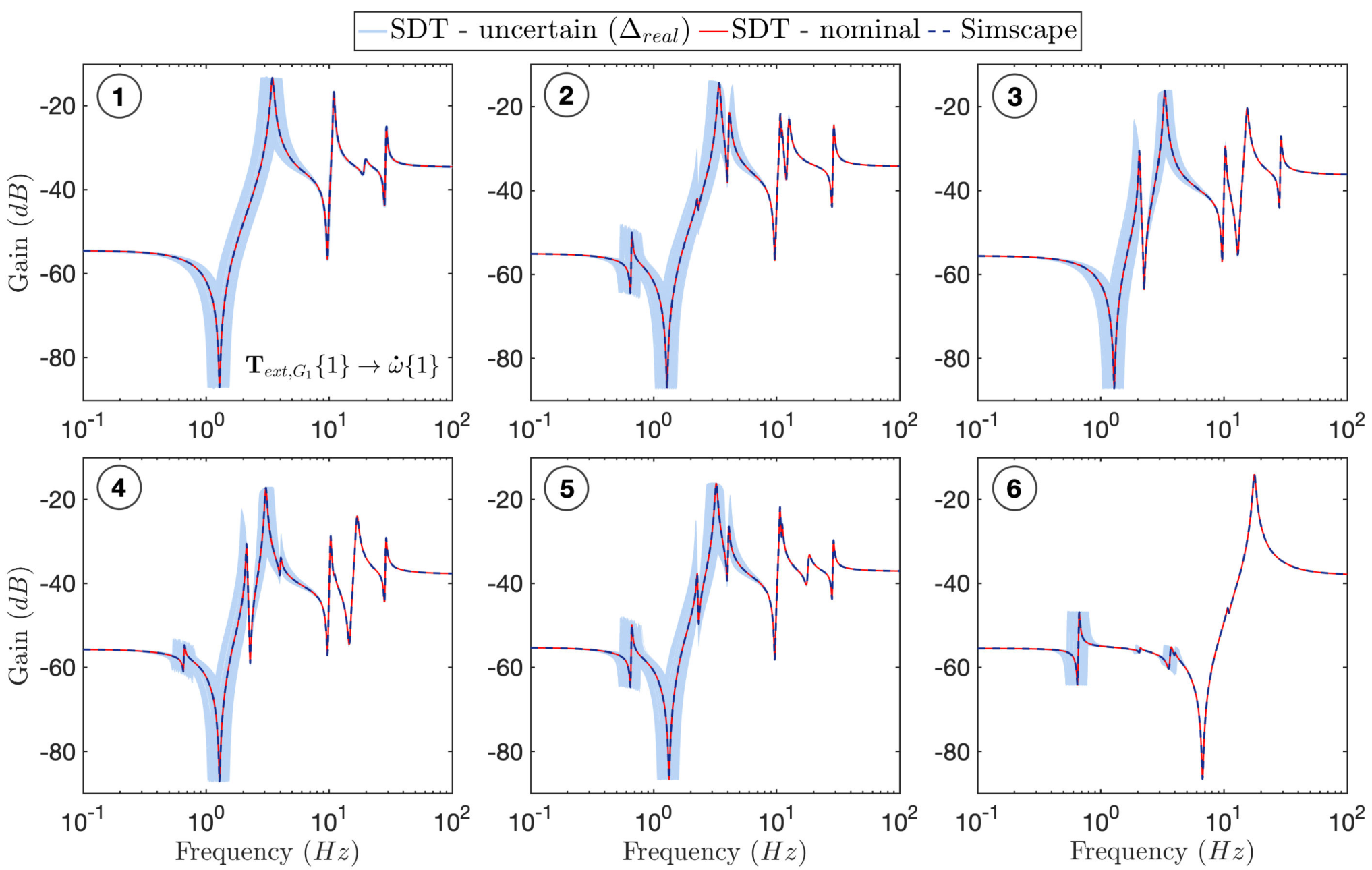
Before proceeding to control design, it has to be ascertained whether the SDT open loop model represented in Fig. 5 and the Simscape system which was built in parallel are identical in the linear domain. Let us now compare the singular values between the Simscape and nominal SDT systems for all six different configurations displayed in Fig. 3 considering the plant shown in Fig. 6. For instance, if the transfer function from the first component of the external torque to the first component of the angular acceleration is considered, Fig. 9 shows an excellent match, since the red and dashed blue lines overlap. The plot is also coherent with the properties of both spacecraft’s flexible elements, in accordance with the modal participation factor matrices definition [30]. Indeed, the antiresonances occur at the frequencies of the cantilevered flexible modes corresponding to the solar arrays. Since SDT computes the inverse linearized dynamic model of the whole system projected in and the channel is being analyzed, the static gains of all the plots in Fig. 9 represent the inverse of the first moment of inertia measured at point and with respect to for all the different moments depicted in Fig. 3.
Furthermore, Fig. 9 also depicts the effect that the set of real parametric uncertainties has on the singular values of the channel . Logically, all the varying tilt angles and are set according to the geometrical configurations that can be observed in the illustrations of Fig. 3. The parametric uncertainties are also replaced accordingly.
Moreover, Fig. 10 assesses the behaviour of the channel when docking happens. For that reason, the LFR models depicted in Fig. 8 are used. The tilt angles and are replaced accordingly and all the modal and mechanical uncertainties are set as nominal. When the damping and stiffness coefficients are very big, a spring-damper system behaves just like a clamped attachment. In addition, when a body docks to another one, the stiffness coefficients are initially small and increase with respect to time.
Fig. 10a shows how the system behaves when the robotic arm docks to the target spacecraft, where the shear and torsional damping coefficients of are equal to or and the stiffness coefficients vary from to or . Since is disconnected, or and or . When are small, the flexible modes of the target’s solar arrays show very small or even non-existent antiresonances/resonances. This can be explained by the fact that the connection to the target is still very weak when are small and therefore the flexible modes do not have a relevant effect on the system dynamics. As the coefficients increase, these resonances and antiresonances start showing up. One of the examples is the antiresonance at around 0.65 , which corresponds to the first flexible mode of the target’s solar arrays. Since or , the six flexible modes which are introduced by are noticeable even when are very big. Logically, as the coefficients increase, there is a shift of these flexible modes to the right, as can be observed in Fig. 10a.
Moreover, Fig. 10b and 10c show both phases of the second docking. First, increase in order to mimic the docking of the target spacecraft to the rigid hub. Then, once this connection is rigid, decrease in order to detach the robotic arm from the target’s rigid hub. The damping coefficients of are equal to or . In this case, the flexible modes which are introduced by do not interfere with the system dynamics for frequencies smaller than 10 . In addition, it can also be observed that the evolution of the system is similar for both cases when increase and when decrease. Another aspect which can be perceived is that the static gain of the singular values plot shown in Fig. 10a is smaller than the one shown in Fig. 10b and 10c. This makes sense since the singular values correspond to the channel and the second moment of inertia of the coupled system measured at point with respect to is bigger in \normalsize7⃝ than in \normalsize8⃝.

2.4 Time-varying analysis
By means of both connection models, this system fully captures the dynamics and interactions between all subsystems as well as the decoupled/coupled configurations. Nevertheless, the trajectories of the robotic arm and solar arrays still need to be defined. With that purpose, fifth-order polynomials are generated, which achieve a given set of input waypoints expressed in terms of joint configurations. The result is displayed in Fig. 11. It should also be noted that the target’s solar panels are considered to be static. Henceforth, and are not represented in Fig. 11 and are both equal to .

The first thing to notice is that the robotic arm starts unfolding during the approach phase, before the first docking occurs at around . Afterwards, the target is attached to the chaser’s bottom surface at . Next, the robotic arm undocks from the target and moves to another configuration. Finally, the chaser’s solar arrays start tilting at . For better analyzing the behaviour of the nominal open loop system, the evolution of the products and moments of inertia with respect to time is obtained and depicted in Fig. 12. It should also be noted that these inertias are measured with respect to . In fact, this plot outlines why it is so fundamental to parameterize the system with respect to its geometrical configuration and to be able to take these inertial changes into account when applying a control methodology. When the first docking occurs, an increase in the moments and products of inertia can be easily observed. However, as the robotic arm moves and brings the target closer to the chaser’s rigid body, the inertia tensor entries start approaching their original values. Around moments \normalsize5⃝ and \normalsize6⃝, some variations can be noticed due to the movement of the solar arrays. Since these rotations happen around and , stays constant.
Moreover, by inspecting the singular values for different frequencies and system configurations, Fig. 13 shows in a clear manner how the system’s flexible modes evolve when the robotic arm moves and the tilt angles of the solar arrays vary. The channel is considered, where denotes the linearized euler angles of the main body with respect to the inertial frame . It should also be noted that is obtained from a double integration of .

Before the first docking, the flexible modes remain practically constant, since the movement of the robotic arm is almost negligible. However, after the first docking occurs at , some of the flexible modes in the mid-range frequency show a very interesting evolution, which can be explained by the fact that the robotic arm is bringing the target spacecraft closer to the chaser’s rigid hub, thus causing great changes in the inertial characteristics of the coupled system. Next, a stabilization can be observed after , since the second docking takes place and the robotic arm movement does not provoke big changes in the mechanical parameters. Finally, when the chaser’s solar arrays start tilting at , a symmetric evolution of some flexible modes can be observed. This behaviour can be explained by the fact that the chaser’s solar arrays are almost symmetric and they undergo a revolution of 180 degrees.
3 Control architecture and synthesis methodology
3.1 Baseline attitude controller
Some of the challenges of an OOS mission scenario include the control structure interactions between the flexible appendages and the AOCS, the time-varying inertial properties, the flexible dynamics, the system uncertainties and also the dynamic couplings. Initially, the control design is divided into two different parts, namely the translational and the attitude. However, only attitude control design is addressed, since this paper’s objective is to focus on the very last phase of the rendezvous between the chaser and target spacecraft. A baseline attitude controller is tuned based on the inertial properties of the coupled system when the first docking takes place at , as follows:
| (10) |
where represents the torque control output and is the angular velocity of the chaser spacecraft defined in with respect to the inertial frame and obtained from integrating . Moreover, is the inertia tensor of the collection of all the body elements, measured with respect to . The objective is to have a critically damped system that returns to rest slowly without oscillating when tracking the reference signals and . For that reason, and represent the controller’s damping ratio and natural frequency, respectively.
The attitude controller is to take action during the complete mission scenario, which involves big changes in the orientation and magnitude of the inertia tensor. Consequently, this tuning methodology is far from appropriate when considering such a challenging and complex scenario. Nevertheless, this controller is useful as an initial guess when using more powerful and advanced control methodologies, such as , which is able to optimize a first approximation until reaching the limits of robustness and performance.
3.2 control
In order to design a control law that accommodates the desired performance requirements, the synthesis problem is recast into the nonsmooth framework [33] by first assembling the weighted interconnection shown in Fig. 14a. First, the plant model represented in Fig. 6 is introduced. However, only the channels are considered, since the objective is to improve the attitude controller. This interconnection is composed of the following blocks:
- 1.
Sensor and actuator models: First, the star tracker dynamics corresponds to a first order low pass filter with a cutoff frequency of 8 . Secondly, the gyroscope dynamics is represented by a first order low pass filter with a 200 cutoff frequency. Finally, the reaction wheel system dynamics is approximated by a second order transfer, with a damping ratio equal to 0.7 and a natural frequency of 200 .
- 2.
Disturbance weights , and : The measurement noise weights and are used to define the upper bounds on the expected spectral amplitude of the closed-loop noise measurements. In this case, and . Similarly, the purpose of the weight is to model the upper bound on the expected closed-loop orbital and robotic arm disturbances at different frequencies. Even though the control loop should include a feedforward term responsible for counteracting the resistance against motion on the locked axes of the joint connecting the robotic arm and the chaser’s rigid hub, some residual constraint torques will still continue to exist. Therefore, the disturbance weight is tuned to take into account these robotic arm disturbances and also orbital perturbations acting on the system, like magnetic or gravity gradient torques.
- 3.
Performance weights and : The purpose of the weight is to impose a desired closed-loop upper bound of 2 on the worst-case actuator signals at different frequencies. Moreover, the Absolute Pointing Error (APE) requirement is given by .
- 4.
Roll-off filter : A 4th-order roll-off Butterworth filter with a cutoff frequency of 0.7 is also added to the output control signal , ensuring the controller is not sensitive to high frequency content.
- 5.
Structured controller : The desired ACS (Attitude Control System) is a static and structured three-by-six controller. All 18 tunable gains are initially set to the values obtained with the baseline controller, which tuning is based on the initial inertial properties of the coupled system. The closed-loop model, denoted , is achieved with the lower linear fractional transformation [28] between the open loop model and the tunable three-by-six controller. This interconnection can be observed in Fig. 14b, where . Ultimately, the uncertain closed-loop model is given by , where represents the upper linear fractional transformation.
First, an array of 200 different plant models is obtained from , by replacing and with 200 equally distributed geometrical configuration waypoints in the time domain. These plant models are obtained with the connection model depicted in Fig. 6, where and are also substituted accordingly. A soft constraint is considered on the norm between the normalized disturbances and outputs of the system, as can be seen below:
| (11) |
Following Eq. (11), any controller for which satisfies the robust performance and stability requirements. The control methodology is finally applied on the array of 200 different plant models, where remains uncertain. In the end, this multimodel control design approach pretends to optimize a controller while taking into account all the big inertia changes that happen during the OOS mission scenario that is being studied. In the case of the optimization shown in Eq. (11), a controller was found to achieve a performance level of , meaning that the soft constraint has been completely satisfied. This control synthesis methodology allows for the design of a structured static controller in one shot, which is able to comply with the imposed requirements for all the different plant models. An in-depth worst-case analysis is now provided in section 4.
4 Performance and stability analysis
4.1 Worst-case analysis
Let us now introduce the structured singular value function [34], which provides very precise information about the magnitude of uncertainty which is needed to destabilize the loop at any frequency [28]. If the nominal system (i.e. the block ) shown in Figure 14b is stable, then the stability of this loop is conditioned by the existence of . This is assessed by evaluating for different frequencies the structured singular value , with being defined for a complex matrix and a set of uncertainties as:
| (12) |
where is the set of -by- complex matrices, represents the maximum singular value of and the set describes the set of finite gain transfer matrices with outputs and inputs. For , the value represents the system gain. If no makes singular, then . Following this definition and under the assumption that the nominal system is stable, then is stable , if and only if: . In this context, gives a measure of the smallest structured uncertainty that causes closed-loop instability for any frequency . Moreover, the gain of this destabilizing perturbation is exactly . This fact will be used to evaluate the stability margin of the loop with respect to different uncertainty structures in the analysis phase. However, due to its non-convex character, can be difficult to compute exactly. For that reason, some very efficient algorithms [35] have been developed in order to estimate the bounds of . In order to assess the stability and performance robustness of the system, two further uncertainties are also considered:
- 1.
Additive uncertainty : The additive uncertainty matrix is an unstructured uncertainty block with a very clear physical interpretation, since it maps the torque signals to the angular acceleration signals . Consequently, essentially covers for unknown inverse dynamic (static or flexible) inertia along the three axes. This 3-by-3 matrix is full (non-zero off-diagonal terms), therefore accounting for possible unknown cross-couplings between the different axes. These imprecisions are covered by the following model :
(13) The weight is used to scale the magnitude of the additive normalized LTI uncertainty block , with .
- 2.
Multiplicative uncertainty : The multiplicative uncertainty block is used to model neglected dynamics, gain fluctuations in the actuators and also phase uncertainty. The new uncertain control torques to the plant are equal to:
(14) where are scalar normalized LTI uncertainties satisfying . In addition, the weights and are used to scale the magnitude of the multiplicative LTI uncertainty blocks and . In addition, it should also be noted that the diagonal terms of the expression are one order of magnitude larger than the off-diagonal terms, with the objective of considering possible couplings due to unmodeled effects or actuator misalignments.
Fig. 15 shows the separate effects of each type of uncertainty on the gains of the transfer function from to regarding the open loop system for moment \scriptsize2⃝.

A new uncertain closed-loop interconnection is obtained using the controller synthesized in the previous section, which is given by , with . A new array of 330 different plant models is obtained from . Similarly to how was accomplished, results from replacing , , and accordingly along 330 equally distributed waypoints in the time domain. In this case, the block remains uncertain.
The robust stability of is finally evaluated. This assessment is done by calculating the bounds on the structured singular value across a dense grid of frequencies , while taking into account all the uncertain 330 plant models. Fig. 16a depicts the upper bounds of for the complete set of considered uncertainties . Furthermore, Fig. 16b illustrates the side views of the upper bounds of the same function with respect to several different sets of uncertainty. The peak of , which corresponds to the minimum in stability margin, occurs around , which means it happens right after the first docking. Furthermore, this peak also occurs for a frequency of 0.55 , which corresponds to the worst-case . However, even when combining all the uncertainty, remains below 0.79 and therefore the loop can tolerate an increase in the uncertainty of 26% while maintaining stability.

The impact of all the subsets of uncertainties was also assessed on different performance indicators using structured singular value computations. Fig. 17 illustrates the upper bounds on the peak gain for different performance signals across frequencies and for . The first performance transfer can be observed in Fig. 17a, which corresponds to the absolute pointing error tracking channel. In this case, the highest peak happens for frequencies around . This peak is mainly caused by the worst-case and , which causes an increase in the gain of the closed-loop system for frequencies around . For , the worst-case gains are mainly sensitive to modal uncertainties . The peaks that occur at 0.59, 0.66 and 0.72 are once again caused by the uncertain natural frequencies . For , some small peaks can be observed in Fig. 17a around the flexible modes’ natural frequencies. However, they do not compromise the tracking performance.
The worst-case gains of a second performance channel corresponding to the maximum control effort are shown in Fig. 17b. It can be observed that the channel maintains values close to nominal ones even in the presence of significant model uncertainty. However, this channel is also slightly sensitive to the presence of modal uncertainties for frequencies around . Indeed, Fig. 17b clearly shows that the highest peak happens around . Afterwards, there is a visible roll-off, which is caused by . The increase in control effort around is once again caused by the worst-case and , which forces the controller to work harder around this frequency.
4.1.1 Stability analysis for the first docking phase
Fig. 10 has shown that taking into account the dynamic behaviour of the docking mechanisms when modeling such a complex system is of paramount importance. Let us now consider the case of Fig. 10a, where the robotic arm is docking to the target, since \normalsize7⃝ represents the most critical docking phase. For that reason, the interconnection displayed in Fig. 14a is now derived by considering the global LFR representation shown in Fig. 8a.
A new uncertain closed-loop interconnection is obtained using the controller synthesized in the previous section, which is given by , with and . A new array of 300 different plant models is obtained from by replacing with 300 systematically increasing values from 0.1 to or and by setting the damping coefficients of as or . Furthermore, and are constant for all the 300 different plant models and set according to the system’s geometrical configuration displayed in \normalsize7⃝.
Fig. 18 depicts the side views of the upper bounds of with respect to . The peak of occurs around or as well as for a frequency equal to 0.58 , which corresponds once again to the worst-case . This peak of is equal to 1.04, what means that the closed-loop can only tolerate 96% of the considered uncertainty while maintaining stability. This stability analysis thus shows the importance of being able to study the behaviour of docking mechanisms, by having spring-damper systems parameterized according to their stiffness and damping characteristics. These LFR models can be taken into account when designing a controller, so that the closed-loop system does not go unstable when docking takes place. Furthermore, these models can also be used for worst-case analysis and controller validation, as it was demonstrated in this section.
This structured singular value analysis can thus be carried out to perform this type of preliminary Validation and Verification cycles on the linearized model of the system. The obtained results can then be utilized to run a guided Monte Carlo simulation where the most problematic areas are explored in more detail. The sensitivity analysis depicted in Fig. 15 can also be used to understand which uncertainties have more impact on the dynamic behaviour of the system. In addition, these results can be used to inform the control and system design process in order to perform quick design iterations. It must be noted that the method described in this paper expects the system to undergo small variations around the linearization point, so that the dynamics remain fairly linear. Since most space missions tend to avoid large deflections and nonlinearities in the structural dynamics by design, this approach covers a vast range of applications. In case relevant nonlinearities are present, which can result from the flexible structures undergoing big deflections, this effect has to be considered during the tuning and validation procedures.
5 Conclusion
This paper outlined a full modeling and control design methodology for an on-orbit servicing scenario. The presented framework shows how to build a very compact representation of the system by taking into account all the elements which make OOS missions so complex and challenging, namely the coupled flexible spacecraft and robotic arm interactions. This modeling process also introduces a new approach using two spring-damper systems with local uncertain damping and stiffness, offering the possibility of modeling the dynamic behaviour of a docking mechanism and also a closed-loop kinematic chain when the robotic arm configuration is static and perfectly known. The controller synthesis procedure includes a thorough description of how to assemble the design model, including all the details related to the different requirements and limits of performance. The posterior robust performance assessment which was performed is a necessary step to ensure the safety and reliability of the proposed control law. The precious information that can be extracted from this analysis can be used to inform the control and system design process. Afterwards, it can also be utilized to perform quick design iterations. This can lead to structural design adjustments or even to the optimization of certain mechanical parameters, like the mass or the inertial properties of a spacecraft. In addition, the possibility to have these Validation and Verification cycles without the need of high computational burden simulations in such a preliminary phase is extremely important.
| Parameter | Description | Value and Uncertainty | |
| Chaser’s rigid hub | distance vector between and written in | m | |
| distance vector between and written in | m | ||
| mass of | |||
| inertia of at written in frame | |||
| Chaser’s solar arrays | distance vector between and written in | ||
| mass of | |||
| inertia of at written in frame | |||
| flexible modes’ frequencies | |||
| flexible modes’ damping | |||
| modal participation factors | |||
| Chaser’s robotic arm | mass of | ||
| x-coordinate of the CoM of written in frame | |||
| y-coordinate of the CoM of written in frame | |||
| z-coordinate of the CoM of written in frame | |||
| first MoI of at the CoM of written in frame | |||
| second MoI of at the CoM of written in frame | |||
| third MoI of at the CoM of written in frame | |||
| first PoI of at the CoM of written in frame | |||
| second PoI of at the CoM of written in frame | |||
| third PoI of at the CoM of written in frame | |||
| Target’s rigid hub | distance vector between and written in | m | |
| mass of | |||
| inertia of at written in frame | |||
| Target’s solar arrays | distance vector between and written in frame | ||
| mass of | |||
| inertia of at written in frame | |||
| flexible modes’ frequencies | |||
| flexible modes’ damping | |||
| modal participation factors |
Funding Sources
This work was funded by ISAE-SUPAERO.
References
- Cumer et al. [2021] C. Cumer, M. Rognant, J.-M. Biannic, C. Roos, Modelling and Attitude Control Design for Autonomous In-orbit Assembly, in: ESA GNC 2021, Sopot, Poland.
- Deremetz et al. [2020] M. Deremetz, P. Letier, G. Grunwald, M. A. Roa, B. Brunner, B. Lietaer, Mosar-wm: A relocatable robotic arm demonstrator for future on-orbit applications.
- Rognant et al. [2019] M. Rognant, C. Cumer, J.-M. Biannic, M. A. Roa, A. Verhaeghe, V. Bissonnette, Autonomous assembly of large structures in space: a technology review, in: EUCASS 2019, Madrid, Spain.
- Crepy-Marglais [2018] J.-D. Crepy-Marglais, Development of a Robust and Combined Controller for On-Orbit Servicing Missions, Ph.D. thesis, 2018.
- Wormnes et al. [2013] K. Wormnes, R. Le Letty, L. Summerer, R. Schonenborg, O. Dubois-Matra, E. Luraschi, A. Cropp, H. Krag, J. Delaval, Esa technologies for space debris remediation, in: 6th European Conference on Space Debris, volume 1, ESA Communications ESTEC Noordwijk, The Netherlands, pp. 1–8.
- Glogowski et al. [2020] M. J. Glogowski, J. D. Anderson, G. A. Herbert, A. D. Kodys, W. A. Llorens, Application of solar electric propulsion in the emerging satellite servicing industry, in: IEPC- 2019.
- Dubanchet et al. [2020a] V. Dubanchet, J. B. Romero, K. N. Gregertsen, H. Austad, J. Gancet, K. Natusiewicz, J. Viñals, G. Guerra, G. Rekleitis, I. Paraskevas, K. Nanos, E. Papadopoulos, L. Majewski, S. Ferraris, J. Purnell, D. Casu, J. D’amico, S. Andiappane, Eross Project-European Autonomous Robotic Vehicle for on-Orbit Servicing, in: i-SAIRAS 2020.
- Dubanchet et al. [2020b] V. Dubanchet, S. Andiappane, P. L. Negro, D. Casu, A. Giovannini, G. Durand, J. D’Amico, Validation and demonstration of EROSS project: The european robotic orbital support services, in: IAC 2020.
- Andiappane et al. [2019] S. Andiappane, G. Durand, V. Dubanchet, Mission and System Design for EROSS project: The European robotic orbital support services, in: IAC 2019.
- Liu et al. [2022] Y. Liu, X. Chen, Y. Zhang, C. Li, Sample data game strategy for active rendezvous with disturbance rejection, Aerospace Science and Technology 121 (2022) 107358.
- Biggs and Brisotto [2021] J. D. Biggs, S. Brisotto, Robust spacecraft rendezvous using a variable speed control moment gyro and thruster, Aerospace Science and Technology 112 (2021) 106644.
- Colagrossi et al. [2021] A. Colagrossi, V. Pesce, L. Bucci, F. Colombi, M. Lavagna, Guidance, navigation and control for 6dof rendezvous in cislunar multi-body environment, Aerospace Science and Technology 114 (2021) 106751.
- Samsam and Chhabra [2022] S. Samsam, R. Chhabra, Multi-impulse smooth trajectory design for long-range rendezvous with an orbiting target using multi-objective non-dominated sorting genetic algorithm, Aerospace Science and Technology 120 (2022) 107285.
- Chai et al. [2020] Y. Chai, J. Luo, N. Han, J. Sun, Robust event-triggered game-based attitude control for on-orbit assembly, Aerospace Science and Technology 103 (2020) 105894.
- Henry et al. [2021] D. Henry, J. Zenteno-Torres, J. Cieslak, A. Ferreira De Loza, J. Dávila, A 6-dof sliding mode fault tolerant control solution for in-orbit autonomous rendezvous, Aerospace Science and Technology 118 (2021) 107050.
- Jonchay et al. [2021] T. S. d. Jonchay, H. Chen, O. Gunasekara, K. Ho, Framework for modeling and optimization of on-orbit servicing operations under demand uncertainties, 2021.
- Moosavian and Papadopoulos [2007] S. A. A. Moosavian, E. Papadopoulos, Free-flying robots in space: An overview of dynamics modeling, planning and control, Robotica 25 (2007) 537–547.
- Brannan and Carignan [????] J. C. Brannan, C. Carignan, Modeling Flexible-Body Dynamics in Real-Time Robotic Systems used in Satellite Servicing Simulations.
- Raina et al. [2021] D. Raina, S. Gora, D. Maheshwari, S. Shah, Impact modeling and reactionless control for post-capturing and manoeuvring of orbiting objects using a multi-arm space robot, Acta Astronautica 182 (2021).
- Wang et al. [2006] J. Wang, R. Mukherji, M. Ficocelli, A. Ogilvie, M. Liu, C. Rice, Modeling and simulation of robotic system for servicing hubble space telescope, pp. 1026–1031.
- Medina et al. [2015] A. Medina, A. Tomassini, M. Suatoni, N. Solway, I. Coxhill, I. Paraskevas, G. Rekleitis, E. Papadopoulos, R. Krenn, A. Brito, B. Sabbatinelli, C. Vidal, O. Benoist, K. Pegg, N. Metzger-Fragnol, G. Visentin, Towards a standardized grasping and refuelling on-orbit servicing for geo spacecraft.
- Sanfedino et al. [2018] F. Sanfedino, D. Alazard, V. Pommier-Budinger, A. Falcoz, F. Boquet, Finite element based n-port model for preliminary design of multibody systems, Journal of Sound and Vibration 415 (2018) 128–146.
- Chebbi et al. [2017] J. Chebbi, V. Dubanchet, J. A. P. Gonzalez, D. Alazard, Linear dynamics of flexible multibody systems : a system-based approach, Multibody System Dynamics 41 (2017) 75–100.
- Sanfedino [2019] F. Sanfedino, Experimental validation of a high accuracy pointing system, Ph.D. thesis, 2019.
- Sanfedino et al. [2021] F. Sanfedino, P. Valentin, D. Oddenino, Integrated modeling of microvibrations induced by solar array drive mechanism for worst-case end-to-end analysis and robust disturbance estimation, Mechanical Systems and Signal Processing 163 (2021) 108168.
- Gonzalez et al. [2016a] J. A. P. Gonzalez, C. Pittet, D. Alazard, T. Loquen, Integrated control/structure design of a large space structure using structured control, in: 20th IFAC Symposium on Automatic Control in Aerospace (ACA 2016), volume 49, Elsevier, Shrerbrooke, CA, 2016a, pp. 302–307.
- Gonzalez et al. [2016b] J. A. P. Gonzalez, D. Alazard, T. Loquen, C. Pittet, C. Cumer, Flexible multibody system linear modeling for control using component modes synthesis and double-port approach, Journal of Dynamic Systems, Measurement, and Control 138 (2016b) 121004.
- Preda et al. [2020] V. Preda, F. Sanfedino, S. Bennani, F. Boquet, D. Alazard, Robust and adaptable dynamic response reshaping of flexible structures, Journal of Sound and Vibration 468 (2020) 115086.
- Alazard and Sanfedino [2021] D. Alazard, F. Sanfedino, Satellite dynamics toolbox library (sdtlib) - user’s guide, 2021.
- Guy et al. [2014] N. Guy, D. Alazard, C. Cumer, C. Charbonnel, Dynamic modeling and analysis of spacecraft with variable tilt of flexible appendages, Journal of Dynamic Systems, Measurement, and Control 136 (2014) 0.
- Dubanchet [2016] V. Dubanchet, Modeling and control of a flexible space robot to capture a tumbling debris, Ph.D. thesis, 2016.
- Kebria et al. [2016] P. M. Kebria, S. Al-wais, H. Abdi, S. Nahavandi, Kinematic and dynamic modelling of ur5 manipulator, in: 2016 IEEE International Conference on Systems, Man, and Cybernetics (SMC), pp. 004229–004234.
- Apkarian and Noll [2006] P. Apkarian, D. Noll, Nonsmooth Synthesis, IEEE Transactions on Automatic Control 51 (2006) 71–86.
- Packard and Doyle [1993] A. Packard, J. Doyle, The complex structured singular value, Automatica 29 (1993) 71–109.
- Balas et al. [2007] G. Balas, R. Chiang, A. Packard, M. Safonov, Robust control toolbox user’s guide, The Math Works, Inc., Tech. Rep (2007).