Multiple Object Trajectory Estimation
Using Backward SimulationThanks: Y. Xia and L. Svensson are with the Department
of Electrical Engineering, Chalmers University of Technology, Gothenburg, Sweden. E-mail: firstname.lastname@chalmers.se. A. F. García-Fernández is with the Department of Electrical Engineering and Electronics, University of Liverpool, Liverpool, United Kingdom, and also with the ARIES research centre, Universidad Antonio de Nebrija, Madrid, Spain. J. L. Williams is with the Commonwealth Scientific and Industrial Research Organization, Brisbane, Australia. D. Svensson is with NVIDIA Corporation, Gothenburg, Sweden. K. Granström is with Embark Trucks Inc., San Francisco, CA, USA.Thanks: The work of D. Svensson was done when he was with Zenseact AB, and the work of K. Granström was done when he was with Chalmers University of Technology.
Abstract
This paper presents a general solution for computing the multi-object posterior for sets of trajectories from a sequence of multi-object (unlabelled) filtering densities and a multi-object dynamic model. Importantly, the proposed solution opens an avenue of trajectory estimation possibilities for multi-object filters that do not explicitly estimate trajectories. In this paper, we first derive a general multi-trajectory backward smoothing equation based on random finite sets of trajectories. Then we show how to sample sets of trajectories using backward simulation for Poisson multi-Bernoulli filtering densities, and develop a tractable implementation based on ranked assignment. The performance of the resulting multi-trajectory particle smoothers is evaluated in a simulation study, and the results demonstrate that they have superior performance in comparison to several state-of-the-art multi-object filters and smoothers.
Index Terms:
Multi-object tracking, random finite sets, sets of trajectories, forward-backward smoothing, backward simulation.I Introduction
Multi-object tracking (MOT) refers to the problem of jointly estimating the number of objects and their trajectories from noisy sensor measurements [1, 2, 3, 4]. Vector-type MOT methods, e.g., the joint probabilistic data association filter (JPDAF) [5] and the multiple hypothesis tracker (MHT) [6, 7], describe the multi-object states and measurements by random vectors; they explicitly estimate trajectories by linking a state estimate with a previous state estimate or declare the appearance of a new object. However, for MOT methods based on sets representation of the multi-object states, e.g., [8, 9, 10, 11], sequences of object states at consecutive time steps cannot be easily constructed.
For these MOT methods, one approach to estimating trajectories is to add a unique label to each single-object state such that each object can be identified over time [12, 13, 14, 15, 16]. This track labelling procedure may work well in some cases, but it often becomes problematic in challenging scenarios, for example, where initially well-separated objects move in close proximity with each other and thereafter separate again [16, 17, 18]. A more advantageous approach to estimating trajectories for filters based on random finite sets (RFSs) [8] is to compute the multi-object posterior on sets of trajectories [17], which captures all the information about the trajectories. This has led to the development of a variety of multi-object trackers: the trajectory probability hypothesis density (PHD) filter [19], the trajectory cardinality PHD filter [19], the trajectory Poisson multi-Bernoulli mixture (PMBM) filter [18], the trajectory multi-Bernoulli mixture (MBM) filter [20], and their approximations the trajectory Poisson multi-Bernoulli (PMB) filter [21] and the trajectory multi-Bernoulli (MB) filter [22]. Note that for RFS-based filters with MB birth, the multi-object posterior may be labelled to consider sets of labelled trajectories [17, 20, 23, 22].

Smoothing for state-space models considers the estimation of object states of interest conditioned on the complete measurement sequence [24]. Therefore, smoothing may provide significantly better object state estimation performance than filtering, by refining earlier object state estimates. Solutions to single-object smoothing in clutter mainly include the Gaussian sum smoother [25, 26, 27, 28, 29], the (integrated) probabilistic data association smoother [30, 31, 32] and the Bernoulli smoother [33, 34, 35]. For vector-type MOT methods with Gaussian filtering, smoothed trajectory estimates are typically obtained by applying a Rauch-Tung-Striebel (RTS) smoother [36] on sequences of single-object filtering densities [37, 38, 39]. It is also possible to consider a batch solution for estimating trajectories using expectation-maximisation [40]. As a comparison, trajectory filters [17, 18, 19, 21, 20, 22, 23] recursively compute the posterior of sets of trajectories as new observations arrive, by performing smoothing-while-filtering [41], and therefore the initiation and termination of estimated trajectories can also be improved.
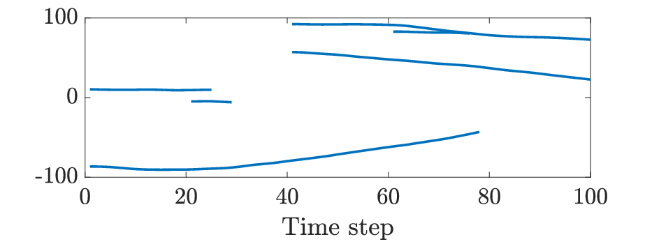
Nevertheless, there are several MOT methods in the literature, e.g., the set JPDAF [42] and the variational PMB filter [43], that can efficiently estimate the multi-object states, but that cannot easily produce smoothed trajectory estimates in a principled manner11 1 A heuristic track-to-target management scheme was presented in [44] by making use of the permutation probabilities of state vectors.. Then an interesting research question arises: “Can we leverage filters that do not keep trajectory information to compute the posterior density of sets of trajectories?”. A one-dimensional example of such trajectory building is illustrated in Fig. 1. Also note that, even for methods that do retain implicit trajectory information, in complex scenarios, approximations made for computational tractability (such as pruning) may cause loss of information that could be recovered with the help of information from later time steps.
In this paper, we show that the exact multi-object posterior of sets of trajectories can be obtained from a sequence of multi-object (unlabelled) filtering densities using the multi-object dynamic model. Specifically, we present a general multi-trajectory backward smoothing equation based on sets of trajectories. The proposed solution has important advantages over multi-object forward-backward smoothers that only compute the marginal multi-object smoothing densities at each time step [45, 46, 47, 48, 49, 50, 51, 52], which, even if labelled, may not be enough to provide meaningful trajectory information [17, Example 2]. Moreover, the proposed forward-backward smoother does not specify the form of the multi-object filtering densities. This is in contrast to multi-object forward-backward smoothers based on labelled RFSs [53, 54, 55], which cannot incorporate the Poisson birth model and require that the multi-object filtering densities must be labelled. The outcome of this work is a method for efficiently sampling multi-object trajectories from the posterior distribution of sets of trajectories, based on operations involving only the single time step multi-object state distributions constructed during forward filtering. This has important applications to offline trajectory analytics, e.g., extracting trajectory estimates that can be viewed as ground truth for the development and verification of perception modules in autonomous driving.
A preliminary version of this work was presented in [56]. This paper is a significant extension of that work, and contains the following contributions:
- 1.
We derive a general multi-trajectory backward smoothing equation based on sets of trajectories.
- 2.
We propose a multi-trajectory particle smoother using backward simulation [57] for PMB filtering densities. In particular, this is a method for doing inference (drawing samples) in the multi-object trajectory space while only ever manipulating single time step, single object marginal distributions, which is only possible because of the properties of the multi-trajectory dynamic model that is stated in Section II-C.
- 3.
We present a tractable implementation of the proposed smoother based on a linear-Gaussian dynamic model and ranked assignment.
- 4.
The rest of the paper is organised as follows. The background on sets of trajectories, multi-object dynamic models and PMB filtering densities is introduced in Section II. The backward smoothing equation for sets of trajectories is presented in Section III. A multi-trajectory particle smoother for PMB filtering densities and its tractable implementation are given in Section IV and Section V, respectively. The simulation results are shown in Section VI, and the conclusions are drawn in Section VII.
II Background
The notation in this paper is defined following the convention in [17, 59]. For a generic space , the set of finite subsets of is denoted by , and the cardinality of a set is . The sequence of ordered positive integers is denoted by , and the set that includes all the permutations of is denoted by . We use to denote union of sets that are mutually disjoint, to denote the inner product , and the multi-object exponential , for some real-valued function , to denote the product with by convention. In addition, we use and to represent the Dirac and Kronecker delta functions centred at , respectively.
II-A State variables
The single-object state is described by a vector , typically containing the kinematic information about the object (e.g., position and velocity). A trajectory is represented as a variable where is the initial time step of the trajectory, is its length, and denotes a finite sequence of length that contains the object states at time steps . For two time steps and , , a trajectory in the time interval existing from time step to satisfies that , and the variable hence belongs to the set . A single trajectory in the time interval therefore belongs to the space . We note that trajectory is a combination of discrete and continuous states. Such a hybrid state is not uncommon in MOT: a typical example is the interacting multiple model [60].
A set of single-object states is a finite subset of , and a set of trajectories is a finite subset of . The subset of trajectories in that were alive at time step where is denoted by
Given a set of trajectories , we denote the resulting set of trajectories in the time interval by
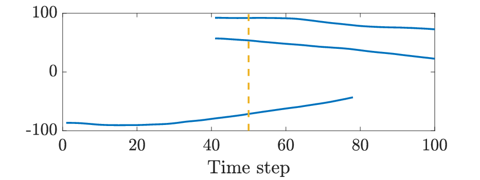
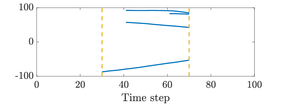
Note that depends on , but we keep this relation implicit for notational clarity. An illustrative example of , and is given in Fig. 2.
Given a single-object trajectory , the set of object states at time step is
and given a set of trajectories, the set of object states at time step is .
II-B Densities and integrals
Given a real-valued function on the single trajectory space , its integral is [17]
| (1) |
which goes through all possible start times, lengths and object states of trajectory . The single trajectory space is locally compact, Hausdorff and second-countable [17], and therefore one can perform inference on sets of finite number of trajectories with finite length [8].
Given a real-valued function on the space of finite sets of trajectories, its set integral is [17]
| (2) |
where . A function on the space is a multi-trajectory density if and its set integral is one.
The multi-object state density at time step and the multi-trajectory density in the time interval , both conditioned on the sequence of sets of measurements received up to and including time step , are denoted by and , respectively. Given a set of object states at time step , the set of trajectories in the time interval is
where trajectory has start time and length with probability one. Therefore, it holds that the multi-trajectory density takes the same value as the multi-object state density when where .
A trajectory Poisson point process (PPP) has density
| (3) |
where is the Poisson intensity, and a trajectory Bernoulli process has density
| (4) |
where is a single-trajectory density and is the probability of existence. A trajectory MB process is the union of independent trajectory Bernoulli components and its density is given by the convolution formula for RFSs [8, Sec. 11.5.3]
| (5) |
where is the density of the -th Bernoulli component, and the sum in (5) goes through all disjoint and possibly empty subsets such that .
Given two single-object trajectories and , the trajectory Dirac delta function is defined as
and the multi-trajectory Dirac delta function centred at is defined as [8, Sec. 11.3.4.3]
II-C Multi-trajectory dynamic model
The conventional multi-object dynamic model described in [8] is considered. Given the current multi-object state , each object survives with probability , and moves to a new state with a Markovian transition density , or dies with probability . The multi-object state at the next time step is the union of the surviving objects and new objects, which are born independently of the rest. The newborn objects are typically modelled as a PPP or an MB process with multi-object state density .
The above conventional multi-object dynamic model results in the following dynamic model for the set of all trajectories that have existed up to the current time step, which will be required in backward smoothing for sets of trajectories. Given a set of all trajectories in the time interval , each trajectory “survives” with probability one, , and moves to a new state according to [17]
| (6) |
That is, if the object underlying trajectory has died before time step , the trajectory remains unaltered with probability one. If trajectory exists at time step , it remains unaltered with probability , or the new final object state is generated according to the single-object transition density with probability . The set of trajectories in the time interval is the union of the dead trajectories, surviving trajectories and new trajectories where each new trajectory has deterministic start time , length , and multi-object state is distributed as .
II-D PMB filtering densities
RFS-based Bayes filters propagate the multi-object posterior density of in time via the prediction and update steps:
| (7) | ||||
| (8) |
where is the multi-object transition density and is the measurement likelihood. For the multi-object dynamic model described in Section II-C with Poisson birth model
| (9) |
where is the Poisson birth intensity at time step , and general multi-object measurement models with Poisson clutter, if the prior is PMBM, the predicted and posterior densities on the current set of object states are PMBM [61]. We note that the Poisson birth model is a special case of PMBM.
The PMB is a common and efficient approximation of a PMBM [11, 43], and its filtering density is defined as
| (10a) | ||||
| (10b) | ||||
| (10c) | ||||
| (10d) | ||||
with . The PMB is the union of two independent RFSs: a PPP with density , parameterised by Poisson intensity , representing undetected objects, and an MB process with density representing detected objects where the -th Bernoulli component has density with probability of existence and single-object state density .
III Backward Smoothing for Sets of Trajectories
In this paper, the objective is to compute the multi-trajectory posterior density using a sequence of multi-object filtering densities with and the multi-trajectory dynamic model via backward smoothing. To achieve this, we first present the multistep prediction theorem for sets of trajectories, which generalises the general prediction theorem for sets of trajectories [17, Theorem 7] to multistep prediction, along with a resulting corollary that is important for the derivation of the general backward smoothing equation for sets of trajectories.
Theorem 1.
Given a multi-trajectory density , its -step predicted multi-trajectory density, with , and , is given by
| (11) |
| (12) |
where we write and denotes the set of trajectories born in the time interval , where is the set of trajectories born at time step with .
Theorem 1 is proved in Appendix A, and it describes that the -step predicted multi-trajectory density of can be evaluated by multiplying the following terms: the multi-trajectory density , for trajectories that died in the time interval , for trajectories that were alive at time step , and the multi-trajectory density for trajectories that appeared after time step .
Corollary 1.1.
For , it holds that
| (13) |
Corollary 1.1 is proved in Appendix B, and it shows that the ratio between the two multi-trajectory densities and does not depend on for .
The general backward smoothing equation for sets of trajectories under the conventional multi-object dynamic model assumptions is presented in the following theorem. Its proof is given in Appendix C.
Theorem 2.
Given the multi-trajectory density and the multi-object state filtering density , the multi-trajectory density in the time interval conditioned on the sequence of sets of measurements up to and including time step is
| (14) |
where the multi-object state predicted density can be computed using via (7), and is the one-step predicted multi-trajectory density of , which takes the same value as .
Theorem 2 shows that the multi-trajectory smoothing density can be expressed as the product of the multi-trajectory smoothing density and the one-step predicted multi-trajectory density of , normalised by the multi-object state predicted density . By applying Theorem 2 recursively backwards in time, we obtain , as desired.
IV A Multi-Trajectory Particle Smoother
In this section, we first introduce a general backward kernel for sets of trajectories, which enables us to perform backward simulation and to approximate the multi-trajectory posterior. Then we present how to evaluate the backward kernel when the multi-object filtering densities are PMB. For the proposed multi-trajectory particle smoother using PMB filtering densities, the forward filtering representations involving single time step, single object marginal distributions can implicitly represent uncertainty over an exponentially large hypothesis space that cannot be feasibly represented through multiple hypothesis methods. The backward simulation framework allows us to draw samples in the multi-object trajectory space from these single time step, single object marginal distributions calculated during the forward filtering which incorporate information from measurements over all the time steps.
IV-A Backward kernel for sets of trajectories
The backward kernel for sets of trajectories is introduced in the following lemma. Its proof is given in Appendix D.
Lemma 3.
The backward kernel for sets of trajectories, i.e., the multi-trajectory density of the set of trajectories in the time interval conditioned on the set of trajectories in the time interval and the sequence of measurement sets up to and including time step , satisfies
| (15) |
Lemma 3 describes that the backward kernel conditioned on the set of trajectories is proportional to the one-step predicted multi-trajectory density only if , and zero otherwise. Note that although the set of trajectories is deterministically given by , evaluating the backward kernel is complicated by the multiple different ways of associating to ; see, e.g., Fig. 1.
In both Theorem 2 and Lemma 3, we consider the distribution of the set of trajectories in the time interval , and we condition on all measurements in the time interval . The main difference between Theorem 2 and Lemma 3 is that the multi-trajectory density computed in Lemma 3 is conditioned on a particular value of the set of trajectories in the time interval , which is what we require for backward simulation.
IV-B Backward kernel for PMB filtering densities
We proceed to present the backward kernel (15) for PMB filtering densities, see (10). We first observe that the backward kernel (15) is in analogy to the Bayesian measurement update (8) in the sense that is the prior and is the measurement likelihood. Specifically, for a PMB filtering density , the one-step predicted multi-trajectory density is a trajectory PMB [21, Lemma 4]. Moreover, the multi-trajectory Dirac delta can be understood as a standard multi-object measurement model [8] with the following characteristics (this will be further elaborated in Appendix E):
- •
Each trajectory is detected with probability
(16) and if detected, it generates a measurement with density .
- •
Clutter is Poisson with intensity .
Then, the backward kernel (15) for PMB filtering densities, obtained via updating the trajectory PMB prior using is a trajectory PMBM [21, Lemma 5]. In what follows, we explain the result of the trajectory PMB update applied to backward simulation with PMB filtering densities, where each trajectory Bernoulli component has information on start/end times of the trajectories giving rise to the following local hypotheses:
- •
The trajectory had never existed in the entire time interval .
- •
The trajectory ended at time step .
- •
The trajectory existed at both time step and .
- •
The trajectory started at time .
We define by the set of indices of trajectories in . Each trajectory in creates a unique trajectory Bernoulli component. The number of trajectory Bernoulli components in is , and they are indexed by variable . A global hypothesis is , where is the number of local hypotheses and is the index to the local hypothesis for the -th trajectory Bernoulli component, which incorporates the following information:
- •
The set of indices . If , then the -th hypothesised trajectory did not appear after time step . If , then the -th hypothesised trajectory existed in the time interval .
- •
The local hypothesis weight (used for computing the probability of the global hypotheses).
- •
The hypothesis-conditioned Bernoulli density of the form (4), parameterised by the probability of existence and the single-trajectory density .
The set of all global hypotheses is
| (17) |
and the weight of global hypothesis satisfies
| (18) |
where the proportionality means that normalisation is required to ensure that . A simple example of the hypothesis structure is illustrated and described in Fig. 3.
The following theorem gives the explicit expression of the PMBM backward kernel (15) for PMB filtering densities.
Theorem 4.
Given a PMB filtering density (10) at time step , the set of trajectories in the time interval and the multi-trajectory dynamic model described in Section II-C with Poisson birth (9), the multi-trajectory density in the time interval conditioned on and the sequence of measurement sets up to and including time step , is a PMBM of the form
| (19) | ||||
| (20) |
| (21) |
where , is given by (18) and
| (22) |
Also, we write with being trajectories of objects that existed at time step , and being trajectories of objects that appeared after time step .
For each trajectory Bernoulli component in the predicted trajectory PMB , , there are local hypotheses. The local hypothesis, corresponding to the case that the trajectory ended at time step , is given by and
| (23a) | ||||
| (23b) | ||||
| (23c) | ||||
The local hypothesis, corresponding to the case that the trajectory Bernoulli component is updated by trajectory , (present at time step , i.e., ), is given by and
| (24a) | ||||
| (24b) | ||||
| (24c) | ||||
The trajectory Bernoulli component created by trajectory , , has two local hypotheses . The first one corresponds to a non-existent Bernoulli and is given by and
| (25) |
The second one is given by and
| (26a) | ||||
| (26b) | ||||
| (26c) | ||||
| (26d) | ||||
| (26e) | ||||
The trajectory Bernoulli component created by trajectory , (not present at time step ) only has a single local hypothesis , given by and
| (27a) | ||||
| (27b) | ||||
| (27c) | ||||
Proof.
See Appendix E. ∎
The local hypothesis parameterised by (25) corresponds to a non-existent Bernoulli component. For a global hypothesis that includes this local hypothesis, trajectory has been assigned to a Bernoulli filtering density. The local hypothesis parameterised by (26) covers the case that the trajectory is associated to the trajectory PPP in ; i.e., the corresponding object was first detected at time step . Note that, for an object that was first detected at time step , it might be born at any time before, or at, time step . Therefore, there is uncertainty on the start time of its corresponding trajectory.
IV-C Backward simulation for sets of trajectories
A particle approximation of the multi-trajectory density is
| (28) |
where is the number of particles and the -th particle has state and weight . By running the backward simulation for sets of trajectories times for where we recursively draw samples of from the backward kernel (15), we can obtain particles representing the multi-trajectory density with uniform weights . Note that, multiple backward set of trajectories can be generated independently, without having to rerun the forward multi-object filter. That is the complexity of backward simulation for sets of trajectories is linear with the number of particles.
For the PMBM backward kernel (19), it is sufficient to sample sets of trajectories described by the MBM (21), which are trajectories of objects that are hypothesised to have been detected at some time, possibly also including object states before their first detection. In other words, we do not sample trajectories of objects that are hypothesised to exist but were never detected. To do so, we first sample a global hypothesis to obtain a trajectory MB, and then we sample a single trajectory state for each Bernoulli component. It is, however, generally intractable to exhaustively enumerate all the global hypotheses. Therefore, approximations are needed for a tractable implementation. One such implementation will be presented for a linear-Gaussian dynamic model in the next section.
V A Tractable Implementation for Linear-Gaussian Dynamic Model
In this section, we present a tractable implementation of the proposed multi-trajectory particle smoother for PMB filtering densities with the following assumptions:
Assumption 1.
The linear Gaussian dynamic model and the PMB filtering densities are defined as follows
- •
The survival probabilities are constant, i.e., .
- •
The linear Gaussian single-object state transition density is where is the state transition matrix and is the motion noise covariance matrix.
- •
The Poisson birth intensity is a Gaussian mixture
(29) where is the number of components, , and are the weight, the mean and the covariance of the -th component, respectively.
- •
The PMB filtering density at time step is parameterised by . Here,
(30) is the Poisson RFS intensity for undetected objects where is the number of components, , and are the weight, the mean and the covariance of the -th component, respectively. In addition, there are Bernoulli components, and the -th component has probability of existence and single-object state density where is its mean and is its covariance.
V-A Gaussian implementation for backward kernel
The backward kernel for sets of trajectories under Assumption 1 is given by the following lemma. For general non-linear dynamic models, the smoothed state density can be computed using Gaussian assumed density approximations [24].
Lemma 5.
Given the linear Gaussian dynamic model, the PMB filtering density at time step specified in Assumption 1 and the set of trajectories in the time interval specified in Theorem 4, the multi-trajectory density in the time interval is a PMBM of the form (19) with and Poisson intensity
| (31) |
The local hypothesis of the -th trajectory Bernoulli component, , corresponding to the case that the trajectory ended at time step , is given by
| (32a) | ||||
| (32b) | ||||
| (32c) | ||||
The local hypothesis of the -th trajectory Bernoulli component, , corresponding to the case that the trajectory Bernoulli component is updated by trajectory , , is given by
| (33a) | ||||
| (33b) | ||||
| (33c) | ||||
| (33d) | ||||
| (33e) | ||||
| (33f) | ||||
| (33g) | ||||
The local hypothesis of the -th trajectory Bernoulli component, , corresponding to the case that the object with trajectory was first detected at time step , is given by
| (34a) | ||||
| (34b) | ||||
| (34c) | ||||
| (34d) | ||||
| (34e) | ||||
| (34f) | ||||
| (34g) | ||||
| (34h) | ||||
| (34i) | ||||
The local hypothesis of the -th trajectory Bernoulli component, , , corresponding to the case that trajectory remains unaltered, has , and .
V-B Practical considerations
The difficulty in drawing samples of sets of trajectories from the trajectory PMBM backward kernel (19) is the number of global hypotheses since enumerating every global hypothesis is of combinatorial complexity. A simple solution is to truncate the MB mixture (21) to only keep global hypotheses with non-negligible weights. This can be achieved by solving a ranked assignment problem using, e.g., Murty’s algorithm [62].
As trajectory Bernoulli components created by trajectories not present at time step all have a single local hypothesis with weight , , the global hypothesis weight (18) becomes
| (35) |
We can then construct the corresponding cost matrix as:
| (36a) | ||||
| (36b) | ||||
| (36c) | ||||
where is a diagonal matrix, and its -th entry is , the weight of associating the -th trajectory to the -th trajectory Bernoulli component. Each global hypothesis can be represented as an assignment matrix consisting of or entries such that each row sums to one and that each column sums to zero or one. Then we obtain the -best global hypotheses that minimise using Murty’s algorithm. Note that the assignment problem formulated here is similar to the assignment problem involved in the PMBM filter update where measurements are associated to Bernoulli/PPP components.
In addition to pruning global hypotheses with small weights, we apply ellipsoidal gating to remove unlikely local hypotheses. Specifically, if the squared Mahalanobis distance between the first state of trajectory , and the predicted density of , i.e.,
is larger than a pre-defined threshold , we then set . This also applies to the Gaussian components of (29) and (30). In addition, clustering can be used to further simplify the computations of the assignment problem.
Having discussed strategies on how to efficiently sample the global hypotheses, we proceed to describe how to simplify the sampling of trajectories from the trajectory Bernoulli densities. We note that a fairly large number of particles may be needed to find the mode of the multi-trajectory density when the Gaussian covariance matrices in (34c) and (33c) are large. A simple heuristic that helps to quickly find the mode in some situations is to approximate each of these Gaussian densities as a Dirac delta centred at its mean. For instance, in this case the single-trajectory density (33c) becomes
and this also avoids the need for computing the corresponding Gaussian covariance (33e).
The robustness of the proposed multi-trajectory particle smoother mainly depends on the number of particles and the maximum number of global hypotheses used in backward simulation. For scenarios with large motion noises or PMB filtering densities with many Bernoulli components, we may need large and to obtain good smoothing performance. In fact, if the computational complexity is not a concern in offline applications (which is usually the case), one can always use larger and to obtain improved results.
Finally, the pseudocode of linear/Gaussian backward simulation for sets of trajectories with PMB filtering densities can be found in Appendix G.
VI Illustrative Example and Simulation Results
In this section, we first illustrate how to perform backward smoothing for sets of trajectories using Theorem 2 via a one-dimensional example shown in Fig. 4a. Then, we evaluate the performance of the proposed multi-trajectory particle smoother for PMB filtering densities in two different two-dimensional scenarios.
VI-A Illustrative example
We consider a one-dimensional scenario on the line segment , of length time steps, where two initially well-separated objects first approach each other (on the real line), then pause for , before crossing each other. In the model, objects survive with probability and new objects appear according to a Poisson birth model with intensity . A nearly constant velocity motion model is used with sampling period and single-object state transition density parameterised by
We also assume that the multi-object filtering density at each time step is a multi-object Dirac delta, which is a special type of PMB with zero PPP intensity and each Bernoulli component having probability of existence one and single target density being a Dirac delta. The ground truth and filtering estimates are illustrated in Fig. 4a.


The objective is to compute the multi-trajectory posterior , which, in this example, can be directly derived using Theorem 2. However, due to the multiple possible associations of single-object Dirac deltas at different time steps, the number of mixture components in the multi-trajectory smoothing density increases very fast when computed backward in time, and thus it soon becomes infeasible to evaluate without approximation. As shown in Appendix H, the multi-trajectory smoothing density has already a mixture representation of 7 components. In this example, we compute the approximate by pruning mixture components with negligible weights. Fig. 4b, 4c and 4d show the estimated sets of trajectories in descending order of posterior probability. The results show that the estimate with unbroken trajectories has the highest weight. With the considered multi-object dynamic model, the set of trajectories with the highest posterior probability closely matches the true trajectories. The other sets of trajectories (with less probability) do not properly link one of the trajectories and, therefore, estimate an additional trajectory.
VI-B Simulation results
We present the results from a Monte Carlo simulation with 500 runs where the performance of the following multi-object filters/smoothers are compared:
- 1.
Track-oriented PMB filter [11], referred to as TO-PMB.
- 2.
Variational PMB filter [43], referred to as V-PMB.
- 3.
Multi-trajectory particle smoother with TO-PMB filtering densities, referred to as BS-TO-PMB.
- 4.
Multi-trajectory particle smoother with V-PMB filtering densities, referred to as BS-V-PMB.
- 5.
Trajectory PMBM filter for the set of all trajectories [18], referred to as T-PMBM.
- 6.
Trajectory PMB filter for the set of all trajectories [21], referred to as T-PMB.
- 7.
-GLMB filter with a multi-scan estimator [58] and RTS smoothing, referred to as GLMB.
- 8.
Multi-scan GLMB with batch smoothing [23], referred to as M-GLMB.
We note that both 7) and 8) can be considered as implementations of the trajectory filter in [17].


We consider a two-dimensional scenario with time steps where six initially well-separated objects move in close proximity to each other and thereafter separate, in the area . The true trajectories of the simulated scenario are illustrated in Fig. 5. We use a nearly constant velocity motion model with sampling period and single-object state transition density parameterised by
where is an identity matrix, denotes the Kronecker product, and . Each object survives with probability . We also consider the point object measurement model where each object generates at most one measurement. The probability of detection is and the clutter is uniformly distributed in the tracking area with Poisson rate . The measurement model is also linear and Gaussian with observation matrix and measurement noise covariance where .
For implementations with Poisson birth model, the Poisson birth intensity is a single Gaussian (c.f. (29)) with parameter , , and . The MB birth model used in GLMB and MS-GLMB contains a single Bernoulli with the same PHD as the Poisson birth process.
All the implementations use ellipsoidal gating (with gating size computed using the inverse-chi-squared distribution at probability 0.9999) to remove unlikely local hypotheses and Murty’s algorithm to find the -best global hypotheses with highest weight, with the only exception being MS-GLMB where the multi-scan data association problem is solved using Gibbs sampling. The maximum number of hypotheses is 100 for TO-PMB, V-PMB and T-PMB, and 1000 for T-PMBM and GLMB. For filters with Poisson birth, Bernoulli components with probability of existence smaller than and Poisson components with weights smaller than are pruned. For T-PMBM and T-PMB, Bernoulli components with probability of being alive at the current time step smaller than are considered dead, and both filters are implemented without -scan approximation, i.e., single-object states at different time steps are not considered independent. For T-PMBM and GLMB, we prune global hypotheses with weight smaller than . For MS-GLMB, the smoothed multi-trajectory estimate obtained from GLMB is used to initialise the Markov chain and 1000 iterations are used in the multi-scan Gibbs sampler. For BS-TO-PMB and BS-V-PMB, the number of particles is 1000 and only a maximum of 100 global hypotheses with weight larger than can be sampled.
For filters with Poisson birth, estimates are extracted from Bernoulli components with probability of existence . For T-PMBM, this is done for the global hypothesis with the highest weight. Also note that we only extract T-PMBM and T-PMB estimates at the last time step. For GLMB and M-GLMB, we also report estimates from the global hypothesis with the highest weight. For BS-TO-PMB and BS-V-PMB, we report the particle (set of trajectories estimate) with the highest likelihood accumulated over time, see Appendix G for implementation details.
The multi-object state estimation performance is evaluated using the generalised optimal sub-pattern assignment (GOSPA) metric [63] with , and . Given a metric in , a scalar , and a scalar with , the GOSPA metric () between sets and is [63, Proposition 1]
where is an assignment set between sets and , and is the set of all possible assignment sets. In addition, the multi-trajectory estimation performance is evaluated using the linear programming (LP) metric for sets of trajectories [64] with , and , which is an extension of GOSPA to sets of trajectories.

| GOSPA | Localisation | Missed | False | |
|---|---|---|---|---|
| TO-PMB | 859.5 | 93.6 | 358.5 | 196.0 |
| BS-TO-PMB | 606.8 | 64.3 | 272.3 | 119.2 |
| V-PMB | 772.0 | 83.3 | 363.8 | 140.0 |
| BS-V-PMB | 55.7 | 226.7 | 78.6 |

| Total | Localisation | Missed | False | Switch | |
|---|---|---|---|---|---|
| BS-TO-PMB | 688.2 | 277.9 | 274.9 | 118.3 | 17.2 |
| BS-V-PMB | 242.6 | 225.2 | 79.0 | 17.7 | |
| T-PMBM | 640.5 | 243.9 | 356.2 | 22.9 | 17.5 |
| T-PMB | 722.3 | 280.3 | 237.8 | 185.9 | 18.3 |
| GLMB | 867.0 | 285.9 | 329.8 | 232.1 | 19.2 |
| M-GLMB | 724.3 | 262.5 | 324.5 | 116.5 | 18.8 |


We first analyse how the two multi-trajectory smoothers can improve multi-object estimation performance with respect to the forward filters. For TO-PMB, BS-TO-PMB, V-PMB and BS-V-PMB, the GOSPA error versus time is shown in Fig. 6, and the average GOSPA error and its decomposition into localisation error, missed detection error and false detection error are presented in Table I. It can be seen from Fig. 6 that TO-PMB shows the largest estimation error when objects moving in close proximity begin to separate, a problem known as track coalescence commonly observed in JPDAF. As a comparison, V-PMB resolves the coalescence by using a more accurate MB approximation method [43]. Both BS-TO-PMB and BS-V-PMB outperform their corresponding forward filters in terms of localisation error, missed and false detections by a large margin. Between these two smoothers, BS-V-PMB has better estimation performance than BS-TO-PMB.
We proceed to analyse the trajectory estimation performance of different implementations. The LP trajectory metric error versus time for all the implementations that estimate trajectories is shown in Fig. 7, and the numerical values of the average LP trajectory metric error are presented in Table II. On the whole, BS-V-PMB has the best estimation performance averaged over different time steps, followed by T-PMBM. In particular, BS-V-PMB has the best performance when objects are in close proximity, whereas T-PMBM has the best performance on initiating and terminating trajectories. In principle, T-PMBM will produce optimal trajectory estimates if it is implemented without approximation, and we apply an optimal estimator (e.g. in the sense of minimising the mean trajectory metric error). However, in practice, we use pruning and a suboptimal estimator. When objects are well-spaced, only hypotheses with negligible weight are pruned, so the performance of T-PMBM is effectively optimal. With closely-spaced objects, there are many feasible hypotheses which cannot be effectively enumerated, and the additional ability of BS-V-PMB to reason over the entire sequence is clearly evident. BS-TO-PMB outperforms T-PMB, with the latter being an efficient approximation of T-PMBM. GLMB is less accurate than the other implementations using Poisson birth model due to their less efficient representation of the multi-object posterior [65], even though for the considered scenario where at most one object is born at a time it is more beneficial to use a Bernoulli birth model. M-GLMB has better performance than GLMB by improving the GLMB estimates using a multi-scan Gibbs sampler with batch smoothing.
The decompositions of the LP trajectory metric error into localisation error, missed detection error, false detection error and track switch error are shown in Fig. 8. T-PMBM, GLMB and M-GLMB show large missed detection errors when objects are in close proximity. In this case, many global hypotheses in T-PMBM and GLMB can have non-negligible weights due to the high data association uncertainty, and capping the number of global hypotheses may result in larger approximation errors than merging multiple global hypotheses into one. This explains why T-PMBM has worse performance than its approximation T-PMB when objects are in close proximity (before separation). Moreover, T-PMBM has very small false detection error, whereas GLMB has difficulty in terminating trajectories of dead objects. T-PMB has less missed detection error but more false detection error than BS-TO-PMB. The track switch error of all the implementations becomes large when objects are in close proximity, and implementations with Poisson birth model have lower track switch error than the two GLMB implementations.
Fig. 9 shows the cardinality distributions of the estimated set of trajectories as well as the trajectory birth and death at different time steps, computed using the particle representations of the multi-trajectory density in BS-V-PMB. As can be seen, these statistics, in general, well reflect the ground truth except at time step 41 when one object died. Specifically, Fig. 9b and Fig. 9c show that it is very likely that no object dies at time step 41.
The average execution times in seconds of a single run22 2 MATLAB implementation on 3.0 GHz Intel Core i5. (81 time steps) for , , , and are: 281.0 (BS-TO-PMB), 209.4 (BS-V-PMB), 171.0 (T-PMBM), 6.5 (T-PMB), 11.1 (GLMB), 8683.7 (M-GLMB). The fastest implementation is T-PMB, followed by GLMB. T-PMBM is slower than GLMB as we do not use the L-scan approximation [21]. BS-V-PMB is faster than BS-TO-PMB even though V-PMB is slower than TO-PMB. This is due to the fact that the computational bottleneck of BS-V-PMB and BS-TO-PMB is backward simulation and that it is faster to run backward simulation on the PMB filtering densities obtained using V-PMB for the considered scenario. M-GLMB is significantly slower than the other implementations as it solves an 81-scan data association problem.
We proceed to analyse the performance of the filters and smoothers with Poisson birth for different scene parameters, and the results are shown in Table III. In general, BS-V-PMB has the best trajectory estimation performance, followed by T-PMBM. As expected, if the scenario has lower signal-to-noise ratio, e.g., when the motion noise or clutter intensity increases, performance of all the filters/smoothers decreases. If the scenario has higher signal-to-noise ratio, e.g., measurement noise or clutter intensity decreases, or probability of detection increases, performance of all the filters/smoothers increases.
| BS-TO-PMB | BS-V-PMB | T-PMBM | T-PMB | |
|---|---|---|---|---|
| No change | 688.2 | 640.5 | 722.3 | |
| 1096.4 | 926.1 | 1088.2 | ||
| 460.5 | 409.8 | 476.4 | ||
| 559.0 | 505.9 | 582.6 | ||
| 642.2 | 565.9 | 668.3 | ||
| 712.1 | 693.2 | 752.2 |

| GOSPA | Localisation | Missed | False | |
|---|---|---|---|---|
| TO-PMB | 281.7 | 24.1 | 192.1 | 11.6 |
| BS-TO-PMB | 96.5 | 15.4 | 33.8 | 3.6 |
| V-PMB | 280.2 | 24.1 | 191.2 | 11.2 |
| BS-V-PMB | 90.7 | 15.4 | 29.8 | 1.8 |
| T-PMBM | 14.4 | 17.0 | 1.2 | |
| T-PMB | 91.5 | 15.7 | 22.8 | 7.7 |
To further demonstrate the ability of the proposed multi-trajectory smoothers to infer object birth locations before first detection, we consider another scenario with time steps where four objects are born at time step 1 and no object dies. Compared to the first scenario, here the probability of detection is and the Poisson clutter rate is . We compare the performance of different implementations with Poisson birth model. The Poisson birth intensity is parameterised by , , , , and the initial Poisson intensity for undetected objects is set to .
The GOSPA error versus time for the considered scenario is shown in Fig. 10 and its decomposition is presented in Table IV. The results show that T-PMBM has the best estimation performance, and that TO-PMB and V-PMB have the worst estimation performance. The estimation performance of T-PMB, BS-TO-PMB and BS-V-PMB is similar, and it is slightly worse than T-PMBM. Due to the low detection probability, objects were usually detected a few time steps after they were born. This explains the high missed detection error of TO-PMB and V-PMB. The estimation of object states before first detection can be obtained by considering the posterior density on sets of trajectories, which captures all the information about the trajectories, including those of undetected objects. For T-PMBM and T-PMB, this information is explicitly carried over time via forward filtering, whereas for BS-TO-PMB and BS-V-PMB, this information is inferred from filtering densities of detected objects at later time steps and gradually recovered via backward smoothing.
At last, we note that the forward-backward smoothers BS-TO-PMB, BS-V-PMB and the trajectory filters T-PMBM, T-PMB are suitable for different applications. BS-TO-PMB and BS-V-PMB are offline methods and their backward smoothing steps do not utilise any information of the measurements and the multi-object measurement model, and therefore they are more suitable for offline trajectory analytics. T-PMBM and T-PMB are online methods, and they can also be applied to batch problems. The difference is that T-PMBM and T-PMB solve the data associations while filtering, whereas with backward simulation, we are not constrained to the previously solved data associations in the sense that future measurements can be utilised to improve trajectory estimation.
VII Conclusions
In this paper, we have derived a multi-trajectory backward smoothing equation based on sets of trajectories. This allows us to leverage filters that do not keep trajectory information to compute the posterior density of sets of trajectories, and has important applications to offline trajectory analytics. In addition, we have proposed a multi-trajectory particle smoother using backward simulation for PMB filtering densities along with its tractable implementation based on ranked assignment. The simulation results show that the proposed methods have superior trajectory estimation performance compared to several state-of-the-art algorithms.
A follow-up work direction is developing an implementation that works for forward densities with particle representation. In addition, it would be interesting to study how to extract better estimates from the particle representation of multi-trajectory densities (28), e.g., by merging different particles in the multi-object trajectory space.
References
- [1] Y. Bar-Shalom, X. R. Li, and T. Kirubarajan, Estimation with applications to tracking and navigation: theory algorithms and software. John Wiley & Sons, 2004.
- [2] S. Challa, M. R. Morelande, D. Mušicki, and R. J. Evans, Fundamentals of object tracking. Cambridge University Press, 2011.
- [3] F. Meyer, T. Kropfreiter, J. L. Williams, R. Lau, F. Hlawatsch, P. Braca, and M. Z. Win, “Message passing algorithms for scalable multitarget tracking,” Proceedings of the IEEE, vol. 106, no. 2, pp. 221–259, 2018.
- [4] R. L. Streit, R. B. Angle, and M. Efe, Analytic combinatorics in multiple object tracking. Springer, 2021.
- [5] Y. Bar-Shalom, F. Daum, and J. Huang, “The probabilistic data association filter,” IEEE Control Systems Magazine, vol. 29, no. 6, pp. 82–100, 2009.
- [6] S. S. Blackman, “Multiple hypothesis tracking for multiple target tracking,” IEEE Aerospace and Electronic Systems Magazine, vol. 19, no. 1, pp. 5–18, 2004.
- [7] C. Chong, S. Mori, and D. B. Reid, “Forty years of multiple hypothesis tracking,” Journal of Advances in Information Fusion, vol. 14, no. 2, pp. 131–151, 2019.
- [8] R. P. Mahler, Statistical Multisource-Multitarget Information Fusion. Artech House Norwood, MA, 2007.
- [9] ——, “Multitarget Bayes filtering via first-order multitarget moments,” IEEE Transactions on Aerospace and Electronic systems, vol. 39, no. 4, pp. 1152–1178, 2003.
- [10] ——, “PHD filters of higher order in target number,” IEEE Transactions on Aerospace and Electronic systems, vol. 43, no. 4, pp. 1523–1543, 2007.
- [11] J. L. Williams, “Marginal multi-Bernoulli filters: RFS derivation of MHT, JIPDA, and association-based member,” IEEE Transactions on Aerospace and Electronic Systems, vol. 51, no. 3, pp. 1664–1687, 2015.
- [12] B.-T. Vo and B.-N. Vo, “Labeled random finite sets and multi-object conjugate priors,” IEEE Transactions on Signal Processing, vol. 61, no. 13, pp. 3460–3475, 2013.
- [13] Á. F. García-Fernández, J. Grajal, and M. R. Morelande, “Two-layer particle filter for multiple target detection and tracking,” IEEE Transactions on Aerospace and Electronic Systems, vol. 49, no. 3, pp. 1569–1588, 2013.
- [14] Á. F. García-Fernández, M. R. Morelande, and J. Grajal, “Bayesian sequential track formation,” IEEE Transactions on Signal Processing, vol. 62, no. 24, pp. 6366–6379, 2014.
- [15] R. Streit, “Analytic combinatorics and labeling in high level fusion and multihypothesis tracking,” in 21st International Conference on Information Fusion (FUSION). IEEE, 2018, pp. 1–5.
- [16] E. H. Aoki, P. K. Mandal, L. Svensson, Y. Boers, and A. Bagchi, “Labeling uncertainty in multitarget tracking,” IEEE Transactions on Aerospace and Electronic systems, vol. 52, no. 3, pp. 1006–1020, 2016.
- [17] Á. F. García-Fernández, L. Svensson, and M. R. Morelande, “Multiple target tracking based on sets of trajectories,” IEEE Transactions on Aerospace and Electronic Systems, vol. 56, no. 3, pp. 1685–1707, 2019.
- [18] K. Granström, L. Svensson, Y. Xia, J. Williams, and Á. F. García-Femández, “Poisson multi-Bernoulli mixture trackers: Continuity through random finite sets of trajectories,” in 21st International Conference on Information Fusion (FUSION). IEEE, 2018, pp. 1–8.
- [19] Á. F. García-Fernández and L. Svensson, “Trajectory PHD and CPHD filters,” IEEE Transactions on Signal Processing, vol. 67, no. 22, pp. 5702–5714, 2019.
- [20] Y. Xia, K. Granström, L. Svensson, Á. F. García-Fernández, and J. L. Williams, “Multi-scan implementation of the trajectory Poisson multi-Bernoulli mixture filter,” Journal of Advances in Information Fusion, vol. 14, no. 2, pp. 213–235, 2019.
- [21] Á. F. García-Fernández, L. Svensson, J. L. Williams, Y. Xia, and K. Granström, “Trajectory Poisson multi-Bernoulli filters,” IEEE Transactions on Signal Processing, vol. 68, pp. 4933–4945, 2020.
- [22] ——, “Trajectory multi-Bernoulli filters for multi-target tracking based on sets of trajectories,” in IEEE 23rd International Conference on Information Fusion (FUSION). IEEE, 2020, pp. 1–8.
- [23] B.-N. Vo and B.-T. Vo, “A multi-scan labeled random finite set model for multi-object state estimation,” IEEE Transactions on Signal Processing, vol. 67, no. 19, pp. 4948–4963, 2019.
- [24] S. Särkkä, Bayesian filtering and smoothing. Cambridge University Press, 2013, no. 3.
- [25] G. Kitagawa, “The two-filter formula for smoothing and an implementation of the Gaussian-sum smoother,” Annals of the Institute of Statistical Mathematics, vol. 46, no. 4, pp. 605–623, 1994.
- [26] D. J. Lee and M. E. Campbell, “Smoothing algorithm for nonlinear systems using Gaussian mixture models,” Journal of Guidance, Control, and Dynamics, vol. 38, no. 8, pp. 1438–1451, 2015.
- [27] A. S. Rahmathullah, L. Svensson, and D. Svensson, “Merging-based forward-backward smoothing on Gaussian mixtures,” in 17th International Conference on Information Fusion (FUSION). IEEE, 2014, pp. 1–8.
- [28] ——, “Two-filter Gaussian mixture smoothing with posterior pruning,” in 17th International Conference on Information Fusion (FUSION). IEEE, 2014, pp. 1–8.
- [29] M. P. Balenzuela, J. Dahlin, N. Bartlett, A. G. Wills, C. Renton, and B. Ninness, “Accurate Gaussian mixture model smoothing using a two-filter approach,” in IEEE Conference on Decision and Control (CDC). IEEE, 2018, pp. 694–699.
- [30] R. Chakravorty and S. Challa, “Augmented state integrated probabilistic data association smoothing for automatic track initiation in clutter,” J. Adv. Inf. Fusion, vol. 1, no. 1, pp. 63–74, 2006.
- [31] T. L. Song and D. Mušicki, “Smoothing innovations and data association with IPDA,” Automatica, vol. 48, no. 7, pp. 1324–1329, 2012.
- [32] D. Mušicki, T. L. Song, and T. H. Kim, “Smoothing multi-scan target tracking in clutter,” IEEE Transactions on Signal Processing, vol. 61, no. 19, pp. 4740–4752, 2013.
- [33] D. Clark, “Joint target-detection and tracking smoothers,” in Signal Processing, Sensor Fusion, and Target Recognition XVIII, vol. 7336. International Society for Optics and Photonics, 2009, p. 73360G.
- [34] B.-T. Vo, D. Clark, B.-N. Vo, and B. Ristic, “Bernoulli forward-backward smoothing for joint target detection and tracking,” IEEE Transactions on Signal Processing, vol. 59, no. 9, pp. 4473–4477, 2011.
- [35] B.-N. Vo, B.-T. Vo, and R. P. Mahler, “Closed-form solutions to forward-backward smoothing,” IEEE Transactions on Signal Processing, vol. 60, no. 1, pp. 2–17, 2011.
- [36] H. E. Rauch, F. Tung, and C. T. Striebel, “Maximum likelihood estimates of linear dynamic systems,” AIAA journal, vol. 3, no. 8, pp. 1445–1450, 1965.
- [37] A. Mahalanabis, B. Zhou, and N. Bose, “Improved multi-target tracking in clutter by PDA smoothing,” IEEE Transactions on Aerospace and Electronic Systems, vol. 26, no. 1, pp. 113–121, 1990.
- [38] W. Koch, “Fixed-interval retrodiction approach to Bayesian IMM-MHT for maneuvering multiple targets,” IEEE Transactions on Aerospace and Electronic Systems, vol. 36, no. 1, pp. 2–14, 2000.
- [39] B. Chen and J. K. Tugnait, “Tracking of multiple maneuvering targets in clutter using IMM/JPDA filtering and fixed-lag smoothing,” Automatica, vol. 37, no. 2, pp. 239–249, 2001.
- [40] A. S. Rahmathullah, R. Selvan, and L. Svensson, “A batch algorithm for estimating trajectories of point targets using expectation maximization,” IEEE Transactions on Signal Processing, vol. 64, no. 18, pp. 4792–4804, 2016.
- [41] M. Briers, A. Doucet, and S. Maskell, “Smoothing algorithms for state-space models,” Annals of the Institute of Statistical Mathematics, vol. 62, no. 1, p. 61, 2010.
- [42] L. Svensson, D. Svensson, M. Guerriero, and P. Willett, “Set JPDA filter for multitarget tracking,” IEEE Transactions on Signal Processing, vol. 59, no. 10, pp. 4677–4691, 2011.
- [43] J. L. Williams, “An efficient, variational approximation of the best fitting multi-Bernoulli filter,” IEEE Transactions on Signal Processing, vol. 63, no. 1, pp. 258–273, 2015.
- [44] D. Svensson, L. Svensson, M. Guerriero, D. F. Crouse, and P. Willett, “The multitarget set JPDA filter with target identity,” in Signal Processing, Sensor Fusion, and Target Recognition XX, vol. 8050. International Society for Optics and Photonics, 2011, p. 805010.
- [45] N. Nandakumaran, K. Punithakumar, and T. Kirubarajan, “Improved multitarget tracking using probability hypothesis density smoothing,” in Signal and Data Processing of Small Targets, vol. 6699. International Society for Optics and Photonics, 2007, p. 66990M.
- [46] D. E. Clark, “First-moment multi-object forward-backward smoothing,” in 13th International Conference on Information Fusion. IEEE, 2010, pp. 1–6.
- [47] N. Nadarajah, T. Kirubarajan, T. Lang, M. McDonald, and K. Punithakumar, “Multitarget tracking using probability hypothesis density smoothing,” IEEE Transactions on Aerospace and Electronic Systems, vol. 47, no. 4, pp. 2344–2360, 2011.
- [48] R. P. Mahler, B.-T. Vo, and B.-N. Vo, “Forward-backward probability hypothesis density smoothing,” IEEE Transactions on Aerospace and Electronic Systems, vol. 48, no. 1, pp. 707–728, 2012.
- [49] P. Feng, W. Wang, S. M. Naqvi, and J. Chambers, “Adaptive retrodiction particle PHD filter for multiple human tracking,” IEEE Signal Processing Letters, vol. 23, no. 11, pp. 1592–1596, 2016.
- [50] D. Li, C. Hou, and D. Yi, “Multi-Bernoulli smoother for multi-target tracking,” Aerospace Science and Technology, vol. 48, pp. 234–245, 2016.
- [51] S. Nagappa, E. D. Delande, D. E. Clark, and J. Houssineau, “A tractable forward-backward CPHD smoother,” IEEE Transactions on Aerospace and Electronic Systems, vol. 53, no. 1, pp. 201–217, 2017.
- [52] R. Streit, “Interval/smoothing filters for multiple object tracking via analytic combinatorics,” in 20th International Conference on Information Fusion (Fusion). IEEE, 2017, pp. 1–8.
- [53] M. Beard, B. T. Vo, and B.-N. Vo, “Generalised labelled multi-Bernoulli forward-backward smoothing,” in 19th International Conference on Information Fusion (FUSION). IEEE, 2016, pp. 688–694.
- [54] R. Liu, H. Fan, T. Li, and H. Xiao, “A computationally efficient labeled multi-Bernoulli smoother for multi-target tracking,” Sensors, vol. 19, no. 19, p. 4226, 2019.
- [55] G. Liang, Q. Li, B. Qi, and L. Qiu, “Multitarget tracking using one time step lagged delta-generalized labeled multi-Bernoulli smoothing,” IEEE Access, vol. 8, pp. 28 242–28 256, 2020.
- [56] Y. Xia, L. Svensson, Á. F. García-Fernández, K. Granström, and J. L. Williams, “Backward simulation for sets of trajectories,” in IEEE 23rd International Conference on Information Fusion (FUSION). IEEE, 2020, pp. 1–8.
- [57] F. Lindsten and T. B. Schön, “Backward simulation methods for Monte Carlo statistical inference,” Foundations and Trends® in Machine Learning, vol. 6, no. 1, pp. 1–143, 2013.
- [58] T. T. D. Nguyen and D. Y. Kim, “GLMB tracker with partial smoothing,” Sensors, vol. 19, no. 20, p. 4419, 2019.
- [59] K. Granström, L. Svensson, Y. Xia, J. Williams, and Á. F. García-Fernández, “Poisson multi-Bernoulli mixtures for sets of trajectories,” arXiv preprint arXiv:1912.08718, 2019.
- [60] H. A. Blom and Y. Bar-Shalom, “The interacting multiple model algorithm for systems with Markovian switching coefficients,” IEEE Transactions on Automatic Control, vol. 33, no. 8, pp. 780–783, 1988.
- [61] Á. F. García-Fernández, J. L. Williams, L. Svensson, and Y. Xia, “A Poisson multi-Bernoulli mixture filter for coexisting point and extended targets,” IEEE Transactions on Signal Processing, vol. 69, pp. 2600–2610, 2021.
- [62] D. F. Crouse, “On implementing 2D rectangular assignment algorithms,” IEEE Transactions on Aerospace and Electronic Systems, vol. 52, no. 4, pp. 1679–1696, 2016.
- [63] A. S. Rahmathullah, Á. F. García-Fernández, and L. Svensson, “Generalized optimal sub-pattern assignment metric,” in Proceedings of International Conference on Information Fusion. IEEE, 2017, pp. 1–8.
- [64] Á. F. García-Fernández, A. S. Rahmathullah, and L. Svensson, “A metric on the space of finite sets of trajectories for evaluation of multi-target tracking algorithms,” IEEE Transactions on Signal Processing, vol. 68, pp. 3917–3928, 2020.
- [65] Á. F. García-Fernández, J. L. Williams, K. Granström, and L. Svensson, “Poisson multi-Bernoulli mixture filter: direct derivation and implementation,” IEEE Transactions on Aerospace and Electronic Systems, vol. 54, no. 4, pp. 1883–1901, 2018.
Supplementary Materials
Appendix A Proof of Theorem 1
We prove Theorem 1 by induction33 3 A direct proof using sets integrals can be found in [56, Appendix A].. The base case one-step prediction with has been proved in [17]. We proceed to show that if (11) and (12) hold, then the -step predicted multi-trajectory density of is also of the form (11) and (12). We define as the set of trajectories born at time step . Then the one-step predicted multi-trajectory density of is
| (37) |
We further write where is the set of trajectories present at time step and is the set of trajectories that appeared after time step (by assumption ). This allows us to separate the product over in (37) into two products over and , respectively. By plugging (11) and (12) into (37) and combining these two products with the product over in (11) and the product over in (12), respectively, we obtain
| (38) |
| (39) |
We can then observe that (38) has the same form as (11), and that (39) has the same form as (12).
This finishes the proof of Theorem 1.
Appendix B Proof of Corollary 1.1
We observe that the only factor in (11) that depends on time step is . This means that the quotient
does not depend on time step , and therefore it holds that
| (40) |
Setting in (40) gives
| (41) |
which can be rearranged to obtain (13).
This finishes the proof of Corollary 1.1.
Appendix C Proof of Theorem 2
Let and be the set of trajectories in the time interval and , respectively. Applying the total probability theorem and Bayes’ rule gives
| (42) |
where defines the backward transition density from to conditioned on the sequence of sets of measurements up to and including time step . Assume that is independent of measurements that are in the future given :
| (43) |
Then we have
| (44) |
Bayes’ rule then yields
| (45) |
where defines the transition density from to , which is a multi-trajectory Dirac delta. The integral over in (45) can then be cancelled out by applying the prediction equation for sets of trajectories [17, Eq. (8)], which gives us
| (46) |
Applying Corollary 1.1 on (46) yields
| (47) |
Appendix D Proof of Lemma 3
We first rewrite using (43) and Bayes’ rule:
| (48) |
where defines the transition density from to , which is a multi-trajectory Dirac delta. We then apply Corollary 1.1, which gives
| (49) |
As does not depend on , we can further express as (15).
This finishes the proof of Lemma 3.
Appendix E Proof of Theorem 4
We first give the explicit expression of the multi-trajectory density . Given the PMB filtering density at time step (cf. (10)) and the multi-trajectory dynamic model described in Section II-C with Poisson birth density (9), the predicted multi-trajectory density is a PMB [21, Lemma 4]
| (50) |
with , where is of the form (3) with intensity
| (51) |
and is of the form (4), parameterised by
| (52) | ||||
| (53) |
where the single trajectory transition density is given by (II-C).
Next, we elaborate on why the multi-trajectory Dirac delta can be seen as a standard multi-object measurement model [8] with characteristics specified in Section IV-B. We note that the multi-trajectory Dirac delta can be written as a trajectory MB where each trajectory Bernoulli component is parameterised by probability of existence one and a Dirac delta single-trajectory density, i.e.,
| (54) |
where for trajectories that did not exist in the time interval , they are implicitly represented by trajectory Bernoulli components with zero probability of existence. Therefore, the multi-trajectory Dirac delta can be understood as a standard measurement model for sets of trajectories [21]:
- •
Each trajectory is detected with probability
(55) and if detected, it generates a measurement with density .
- •
Poisson clutter intensity .
Note that if a trajectory in the time interval did not exist in the time interval , then it must have start time and length .
Having established the analogy between the backward kernel (15) for PMB filtering densities and the trajectory PMB update, the explicit expression of the trajectory PMBM backward kernel (19) can be straightforward obtained by plugging the trajectory PMB prior (50) and measurement model (54) into the trajectory PMB update equations [21, Lemma 5]. One thing to be noted is that the set of trajectories appeared after time step remains unaltered. This will be further elaborated.
We write as the disjoint union of the set of trajectories present at time step or and the set of trajectories of objects that appeared after time step . We also write as the disjoint union of the set of trajectories of objects that existed at time step and the set of trajectories of objects that appeared after time step . It holds that by construction, and that the density of conditioned on is zero unless . Then we have
| (56) |
and the backward kernel (15) becomes
| (57) |
where can be written as a trajectory MB similar to (54). This explains the last part of Theorem 4 and finishes the proof of Theorem 4.
Appendix F
For the particle representation of the multi-trajectory density (28), the cardinality distribution of the set of trajectories is given by
| (58) |
the cardinality distribution of the trajectories born at time step with is given by
| (59) |
and the cardinality distribution of the trajectories that die at time step with is given by
| (60) |
Appendix G
The pseudocode of linear-Gaussian backward simulation for sets of trajectories with PMB filtering densities along with an efficient estimator is given in Algorithm 1. The proposed estimator reports the particle with the highest likelihood accumulated over time from particles (sets of trajectories) with equal weight .
Appendix H
In this appendix, we derive the explicit expression of multi-trajectory smoothing density for the one-dimensional example in Section VI-A.
We write where the set of trajectories present at both time step and , the set of trajectories only present at time step , and the set of trajectories only present at time step . We also write the multi-object filtering density at time step as where and . The predicted multi-trajectory density of for each of the events can then be expressed using Theorem 1:
- •
The two objects existed at both time step and ,
- •
Object with state existed at time step and object with state died at time step ,
- •
Object with state existed at time step and object with state died at time step ,
- •
The two objects died at time step ,
When taking the product of the two multi-trajectory densities and , a multi-trajectory Dirac delta with two components, each of the first three events has two different cases due to the unknown correspondence between and . Therefore, the multi-trajectory density has a mixture representation of components.