Closed-Form Diffeomorphic Transformations for Time Series Alignment
Abstract
Time series alignment methods call for highly expressive, differentiable and invertible warping functions which preserve temporal topology, i.e diffeomorphisms. Diffeomorphic warping functions can be generated from the integration of velocity fields governed by an ordinary differential equation (ODE). Gradient-based optimization frameworks containing diffeomorphic transformations require to calculate derivatives to the differential equation’s solution with respect to the model parameters, i.e. sensitivity analysis. Unfortunately, deep learning frameworks typically lack automatic-differentiation-compatible sensitivity analysis methods; and implicit functions, such as the solution of ODE, require particular care. Current solutions appeal to adjoint sensitivity methods, ad-hoc numerical solvers or ResNet’s Eulerian discretization. In this work, we present a closed-form expression for the ODE solution and its gradient under continuous piecewise-affine (CPA) velocity functions. We present a highly optimized implementation of the results on CPU and GPU. Furthermore, we conduct extensive experiments on several datasets to validate the generalization ability of our model to unseen data for time-series joint alignment. Results show significant improvements both in terms of efficiency and accuracy.
Keywords:
time series, nonlinear time warping, diffeomorphisms, machine learning, deep learning, nearest centroid classification, time series averaging, temporal distortion, time series analysis, sensitivity analysis, ordinary differential equations1 Introduction and Context
Time series data recurrently appears misaligned or warped in time despite exhibiting amplitude and shape similarity. Temporal misalignment, often caused by differences in execution, sampling rates, or the number of measurements, confounds statistical analysis to the point where even the sample mean of semantically-close time series can obfuscate actual peaks and valleys, generate non-existent features and be rendered almost meaningless. Indeed, ignoring temporal variability can greatly decrease recognition and classification performance (Veeraraghavan et al. 2009).
Time series alignment can be solved by finding a set of optimal and plausible warping functions between observations of the same process so that their temporal variability is minimized. Alignment methods have become critical for many applications involving time series data, such as bioinformatics, computer vision, industrial data, speech recognition & synthesis, or human action recognition (Srivastava & Klassen 2016). Temporal warping functions extend from low dimensional global transformations described by a few parameters (e.g. affine transformations) to high dimensional non-rigid transformations specified at each point of the domain (e.g. diffeomorphisms). A () diffeomorphism is a differentiable invertible map with a differentiable inverse (Duistermaat & Kolk 2000). Diffeomorphisms belong to the group of homeomorphisms that preserve topology by design, and thereby are a natural choice in the context of nonlinear time warping, where continuous, differentiable and invertible functions are preferred (Mumford & Desolneux 2010; Rivet & Cohen 2016). Diffeomorphic warping functions can be generated via integration of regular stationary or time-dependent velocity fields specified by the ordinary differential equation (ODE) (Freifeld et al. 2017; Detlefsen et al. 2018; van der Ouderaa et al. 2021).
Temporal alignment problems have been widely stated as the estimation of diffeomorphic transformations between input and output data (Huang et al. 2021). Finding the optimal warping function for pairwise or joint alignment requires solving an optimization problem. However, aligning a batch of time series data is insufficient because new optimization problems arise as new data batches arrive. Inspired by Spatial Transformer Networks (STN), Temporal Transformer Networks (TTN) such as (Weber et al. 2019; Lohit et al. 2019; Nunez & Joshi 2020) and recently (Huang et al. 2021), generalize inferred alignments from the original batch to the new data without having to solve a new optimization problem each time. Temporal transformer’s neural network training proceeds via gradient descent on model parameters. Under such gradient-based optimization frameworks, neural networks that include diffeomorphic transformations require to calculate derivatives to the differential equation’s solution with respect to the model parameters, i.e. sensitivity analysis. Unfortunately, deep learning frameworks typically lack automatic-differentiation-compatible sensitivity analysis methods; and implicit functions, such as the solution of ODE, require particular care. Current solutions appeal to adjoint sensitivity methods (Chen et al. 2019), ResNet’s Eulerian discretization (Huang et al. 2021) or ad-hoc numerical solvers and automatic differentiation (Freifeld et al. 2017). More on this in Section 2.
In contrast, our proposal is to formulate the closed-form11 1 A closed-form expression may use a finite number of standard operations (), and functions (e.g., , , , , ) , but no limit, differentiation, or integration. expression for the ODE’s diffeomorphic solution and its gradient under continuous piecewise-affine (CPA) velocity functions. CPA velocity functions yield well-behaved parametrized diffeomorphic transformations, which are efficient to compute, accurate and highly expressive (Freifeld et al. 2015). These finite-dimensional transformations can handle optional constraints (zero-velocity at the boundary) and support convenient modeling choices such as smoothing priors and coarse-to-fine analysis. The term “piecewise” refers to a partition of the temporal domain into subintervals. The fineness of the partition controls the trade-off between expressiveness and computational complexity. Unlike other spaces of highly-expressive velocity fields, integration of CPA velocity fields is given in either closed form (in 1D) or “essentially” closed form for higher dimensions (Freifeld et al. 2017). However, the gradient of CPA-based transformations is only available via the solution of a system of coupled integral equations (Freifeld 2018). Following the first principle of automatic differentiation — if the analytical solution to the derivative is known, then replace the function with its derivative—, in this work we present a closed-form solution for the ODE gradient in 1D that is not available in the current literature.
A closed-form solution provides efficiency, speed and precision. Fast computation is essential if the transformation must be repeated several times, as is the case with iterative gradient descent methods used in deep learning training. Furthermore, a precise (exact) gradient of the transformation translates to efficient search in the parameter space, which leads to better solutions at convergence. Encapsulating the ODE solution (forward operation) and its gradient (backward operation) under a closed-form transformation block shortens the chain of operations and decreases the overhead of managing a long tape with lots of scalar arithmetic operations. Indeed, explicitly implementing the backward operation is more efficient than letting the automatic differentiation system naively differentiate the closed-form forward function.
Furthermore, we integrate closed-form diffeomorphic transformations into a temporal transformer network (see Figure 3) for time series alignment. Similarly to (Weber et al. 2019), we formulate the joint alignment problem as to simultaneously compute the centroid and align all sequential data within a class, under a semi-supervised schema.
Contributions
- •
We propose a novel closed-form expression for the gradient of CPA-based one-dimensional diffeomorphic transformations, providing efficiency, speed and precision.
- •
We present Diffeomorphic Fast Warping (DIFW), an open-source library and highly optimized implementation of 1D diffeomorphic transformations on multiple backends for CPU (NumPy and PyTorch with C++) and GPU (PyTorch with CUDA). Speed tests show an x18 (x260) and x10 (x30) improvement on CPU (GPU) over current solutions for forward and backward operations respectively.
- •
We incorporate these improvements into a diffeomorphic temporal transformer network resembling (Weber et al. 2019) for time-series alignment and classification.
- •
We conduct extensive experiments on 84 datasets from the UCR archive (Dau et al. 2019) to validate the generalization ability of our model to unseen data for time-series joint alignment. Results show significant improvements both in terms of efficiency and accuracy (see Figure 1).
The paper is structured as follows. We discuss related work in Section 2 and outline the mathematical formalism relevant to our method in Section 3. The experiments with extensive results are described in Section 4 and final remarks are included in Section 5.
2 Related Work
2.1 Time Series Alignment
Pairwise alignment: Given two time series observations y and z: , where is the temporal domain, the goal of pairwise alignment is to compute an optimal transformation , such than the data fit between the query y and transformed target is high, that is, their difference according to a distance measure is minimum22 2 The operator refers to function composition. This problem is typically solved as an optimization problem. The “goodness” of the transformation is measured by a cost of the form: . The set is the set of all monotonically-increasing functions from to itself. The first term evaluates the similarity between y and , whereas the second term imposes constraints on the warping function , as smoothness, monotonicity preserving and boundary conditions.
Dynamic Time Warping (DTW) (Sakoe & Chiba 1978) is a popular method that finds the optimal alignment by first computing a pairwise distance matrix and then solving a dynamic program using Bellman’s recursion with a quadratic cost. However, DTW is not differentiable everywhere, is sensitive to noise and leads to bad local optima when used as a loss (Blondel et al. 2021). SoftDTW (Cuturi & Blondel 2017) is a differentiable loss function that replaces the minimum over alignments in DTW with a soft minimum, which induces a probability distribution over alignments.
Joint alignment: Given a set of time series observations the goal of joint alignment is to find a set of optimal warping functions such that the average sequence, , minimizes the sum of distance to all elements in the set : .
DTW Barycenter Averaging (DBA) (Petitjean et al. 2011) minimizes the sum of the DTW discrepancies to the input time-series and iteratively refines an initial average sequence. Generalized Time Warping (GTW) (Zhou & De La Torre 2012) approximates the optimal temporal warping by a linear combination of monotonic basis functions and a Gauss-Newton-based method is used to learn the weights of the basis functions. However, GTW requires a large number of complex basis functions to be effective. (Kawano et al. 2020) relaxed the DTW-based discrete formulation of the joint alignment problem to a continuous optimization in which a neural network learns the optimal warping functions. Also related is the square-root velocity function (SRVF) representation (Srivastava et al. 2011) for analyzing shapes of curves in euclidean spaces under an elastic metric that is invariant to reparametrization. Note that these solutions are cast as an optimization problem, and as a result, lack a generalization mechanism and must compute alignments from scratch for new data.
Temporal Transformer Networks can generalize inferred alignments from the original batch to the new data without having to solve a new optimization problem each time. Diffeomorphisms have been actively studied in the field of image registration and have been successfully applied in a variety of methods (Beg et al. 2005; Vercauteren et al. 2009; Dalca et al. 2018; Fu et al. 2020), such as the log-Euclidean polyaffine method (Arsigny et al. 2006a; Arsigny et al. 2006b). Hereof (Detlefsen et al. 2018) first implemented flexible CPA-based diffeomorphic image transformations within STN, and were later extended to variational autoencoders (Detlefsen & Hauberg 2019). On this subject, (van der Ouderaa et al. 2021) presented an STN with diffeomorphic transformations and used the scaling-and-squaring method for solving 2D stationary velocity fields and the Baker-Campbell-Hausdoorff formula for solving time-dependent velocity fields.
The counterpart STN model for time series alignment is Diffeomorphic Temporal Alignment Nets (DTAN) (Weber et al. 2019) and its recurrent variant R-DTAN. DTAN closely resembles the TTN model presented in this paper, even though the core diffeomorphic transformations are computed differently, as presented in Section 3. In this regard, (Lohit et al. 2019) generated input-dependent warping functions that lead to rate-robust representations, reduce intra-class variability and increase inter-class separation.
Also related is (Rousseau et al. 2019), a residual network for the numerical approximation of exponential diffeomorphic operators. The velocity field in this model is a linear combination of basis functions which are parametrized with convolutional and ReLu layers. Very recently, (Huang et al. 2021) proposed a residual network (ResNet-TW) that echoes an Eulerian discretization of the flow equation (ODE) for CPA time-dependent vector fields to build diffeomorphic transformations. As an alternative approach, (Nunez & Joshi 2020) proposed a deep neural network for learning the warping functions directly from DTW matches, and used it to predict optimal diffeomorphic warping functions. Regarding the SRVF framework, (Nunez et al. 2021) presented an unsupervised generative encoder-decoder architecture (SRVF-Net) to produce a distribution space of SRVF warping functions for the joint alignment of functional data. Beyond diffeomorphic transformations, Trainable Time Warping (Khorram et al. 2019) performs alignment in the continuous-time domain using a sinc convolutional kernel and a gradient-based optimization technique.
2.2 Computing Derivatives to ODE’s solution
In this section we review available solutions to compute derivatives to the ODE’s solution:
Numerical differentiation should be avoided because it requires two numerical ODE solutions for each parameter (very inefficient) and is prone to numerical error: if the step size is too small, it may exhibit floating point cancellation; if the step size is chosen too large, then the error term of the approximation is large.
Forward-mode continuous sensitivity analysis extends the ODE system and studies the model response when each parameter is varied while holding the rest at constant values. However, since the number of ODEs in the system scales proportionally with the number of parameters, this method is impractical for systems with a large number of parameters.
Residual networks (ResNets) can be interpreted as discrete numerical integrators of continuous dynamical systems, with each residual unit acting as one step of Euler’s forward method. ResNet-TW (Huang et al. 2021) use this Eulerian discretization schema of the ODE to generate smooth and invertible transformations. The gradient is computed using reverse-mode AD backpass, also known as backpropagation. However, ResNets are difficult to compress without significantly decreasing model accuracy, and do not learn to represent continuous dynamical systems in any meaningful sense (Queiruga et al. 2020). Even though highly expressive diffeomorphic transformations can be generated via non-stationary velocity functions, the integration error is proportional to the number of residual units. Computing precise ODE solutions with ResNets require increasing the number of layers and as a result, the memory use of the model.
Neural ODEs (Chen et al. 2019), the continuous version of ResNets, compute gradients via continuous adjoint sensitivity analysis, i.e. solving a second augmented ODE backwards in time. The efficiency issue with adjoint sensitivity analysis methods is that they require multiple forward ODE solutions, which can become prohibitively costly in large models. Neural ODEs reduce the computational complexity to a single solve, while retaining low memory cost by solving the adjoint gradients jointly backward-in-time alongside the ODE solution. However, this method implicitly makes the assumption that the ODE integrator is time-reversible and sadly there are no reversible adaptive integrators for first-order ODEs solvers, so this method diverges on some systems (Rackauckas et al. 2019). Other notable approaches for solving the adjoint equations with different memory-compute trade-offs are interpolation schemes (Daulbaev et al. 2020), symplectic integration (Zhuang et al. 2021), storing intermediate quantities (Zhang & Sandu 2014) and checkpointing (Zhuang et al. 2020).
Discrete sensitivity analysis calculates model sensitivities by directly differentiating the numerical method’s steps. Yet, this approach requires specialized implementation of the first-order ODE solvers to propagate said derivatives. Automatic differentiation (AD) can be used on a solver implemented fully in a language with AD (a differential programming approach) (Ma et al. 2021). However, pure tape-based reverse-mode AD software libraries (such as PyTorch (Paszke et al. 2019), ReverseDiff.jl (Revels 2020) and Tensorflow Eager (Agrawal et al. 2019)), have been generally optimized for large linear algebra and array operations, which decrease the size of the tape in relation to the amount of work performed. Given that ODEs are typically defined by nonlinear functions with scalar operations, the tape handling to work ratio gets cut down and is no longer competitive with other forms of derivative calculations (Ma et al. 2021). Other frameworks, such as JAX (Bradbury et al. 2018) cannot JIT optimize the non-static computation graphs of a full ODE solver. These issues may be addressed in the next generation reverse-mode source-to-source AD packages like Zygote.jl (Innes 2018) or Enzyme.jl (Moses & Churavy 2020) by not relying on tape generation.
3 Method
Time series alignment seeks to find a plausible warping function that minimizes the observed temporal variability. We propose spaces of diffeomorphic warping transformations that are based on fast and exact integration of CPA velocity fields. For this section, we inherit the notation used by (Freifeld et al. 2015; Freifeld et al. 2017), who originally proposed CPA-based diffeomorphic transformations.
3.1 CPA Velocity Functions
Let be the Cartesian product of 1D compact intervals that represents the temporal domain.
Definition 3.1.
A finite tessellation is a set of closed subsets of , also called cells , such that their union is and the intersection of any pair of adjacent cells is their shared border. Notation: is the number of cells, number of vertices and number of shared vertices (all three quantities positive integers).
Fix a tessellation , let and define the membership function , . If is not on an inter-cell border, then .
Definition 3.2.
A map is called piecewise affine (PA) w.r.t if are affine, i.e., where . Let’s define , then .
Definition 3.3.
is called CPA if it is continuous and piecewise affine.
Let be the spaces of CPA velocity fields on w.r.t and its dimensionality. A generic element of is denoted by where
The vectorize operation computes the row by row flattening to a column vector. If then . Also, if then , as follows:
Continuity Constraints
Since matrix A defines a CPA transformation, must satisfy a linear system of constraints to be continuous everywhere: where L is the constraint matrix. For a detailed explanation on this matter we refer the reader to Appendix A. The null space of L coincides with the CPA vector-field space. Let be the orthonormal basis of the null space of L. Under this setting, are the coefficients (parameters) of each basis vector, and we can compute the matrix A as follows: . If the velocity field is built using the orthonormal basis B such that , then is CPA.
In this work, we implement four different methods to obtain the null space of L: SVD decomposition, QR decomposition, Reduced Row Echelon Form (RREF) and Sparse Form. We refer the reader to Appendix C for a comparison of these four spaces about sparsity and computation times.
Additional Constraints
To allocate additional constraints, we must extend the constraint matrix L to have more rows. The null space of the extended is a linear subspace of the null space of the original L. For instance, constraining the velocity field to be zero at the border of : (zero-boundary constraint) adds two additional equations (one at each limit of ), thus the number of constraints and basis
Smoothness Priors
We include smoothness priors on CPA velocity functions as done by (Freifeld et al. 2017): First sampling a zero-mean gaussian with covariance matrix whose correlations decay with inter-cell distances ; and then projecting it into the CPA space: . With this procedure we can sample transformation parameters from a prior distribution: , where uses the squared exponential kernel and has two parameters: which controls the overall variance and which controls the kernel’s length-scale. Small generate close to the identity warps and vice versa. Large favors purely affine velocity fields.
3.2 CPA Diffeomorphic Transformations
Definition 3.4.
A map is called a () diffeomorphism on if exists and both and are differentiable. A diffeomorphism can be obtained, via integration, from uniformly continuous stationary velocity fields where for uniformly continuous and integration time .
Any continuous velocity field, whether piecewise-affine or not, defines differentiable trajectories. Let
such that and solves the integral equation:
| (1) |
or, the equivalent ordinary differential equation (ODE):
| (2) |
This integral equation should not be confused with the piecewise-quadratic map, . Both and are not piecewise quadratic.
| (5) |
Letting vary and fixing , is an transformation. Without loss of generality, we may set and define where . The solution to this ODE is the composition of a finite number of solutions :
| (3) |
where is the number of cells visited and is the solution of a basic ODE with an affine velocity field: and an initial condition . The integration details for this ODE are included in Appendix D.
3.3 Closed-Form Integration
Step 1: Given inputs , , and the membership function , compute the cell index and the cell boundary points
Step 2: Calculate the hitting time at the boundary :
Step 3: If then , otherwise repeat from step 1, with new values for , and
This is an iterative process until convergence. The upper bound for is , where refers to the first visited cell index.
3.4 Closed-Form Derivatives of w.r.t.
Let’s recall that the trajectory (the solution for the integral equation 1) is a composition of a finite number of solutions , as given by Equation 3. During the iterative process of integration, several cells are crossed, starting from cell at integration time , and finishing at cell at integration time . The integration time of the last cell can be calculated by subtracting from the initial integration time the accumulated boundary hitting times: . The final integration point is the boundary of the penultimate cell : . In case only one cell is visited, both time and space remain unchanged: and . Taking all of this into account, the trajectory can be calculated as follows:
| (4) |
Therefore, the derivative can be calculated by going backwards in the integration direction. We are interested in the derivative of the trajectory w.r.t. the parameters . Equation 5 shows the expression for the partial derivative w.r.t. one of the coefficients of , i.e., . We refer the reader to Appendices F and G for the corresponding detailed mathematical derivations.
3.5 Scaling-and-Squaring
We use the scaling-and-squaring method (Moler & Van Loan 2003; Higham 2009) to approximate the numerical or closed-form integration of the velocity field. This method uses the following property of diffeomorphic transformations to accelerate the computation of the integral: . Namely, computing the transformation at time is equivalent to composing the transformations at time and . The scaling-and-squaring method imposes , so it only needs to compute one transformation and self-compose it: . Repeating this procedure multiple times (N) we can efficiently approximate the integration:
| (6) |
This procedure relates to the log-euclidean framework (Arsigny et al. 2006a; Arsigny et al. 2006b) that uses (inverse) scaling and squaring for exponential (logarithm) operation on velocity fields.
3.6 Temporal Transformer Network (TTN) Model
The proposed model resembles the Spatial Transformer Network proposed by (Jaderberg et al. 2015), later adapted for time series alignment by (Oh et al. 2018; Lohit et al. 2019; Weber et al. 2019) (see Figure 3), and can recurrently apply nonlinear time warps to the input signal. Composing warps increases the expressiveness without refining as it implies non-stationary velocity functions which are CPA in and piecewise constant in time. Note that unlike (Weber et al. 2019), in our model the localization network parameters are not shared across layers. The differentiable sampler uses piecewise linear interpolation to estimate the warped signals. We refer the reader to Appendix H for details about the sampler estimation and its derivatives.
Loss function
Let denote an input signal among time series samples, and denote the corresponding output of the localization network , and let denote the result of warping by , where depends on w and . The variance of the observed is partially explained by the latent warps , so we seek to minimize the empirical variance of the warped signals:
| (7) |
where is the norm. For multi-class problems, the expression is the sum of within-class variances:
| (8) |
where is the number of classes, takes values in and is the class label associated with and is the number of examples in class . Hence, we formulate the joint alignment problem as to simultaneously compute the centroid and align all sequential data within a class, under a semi-supervised schema: A single net learns how to perform joint alignment within each class without knowing the class labels at test time. Thus, while the within-class alignment remains unsupervised (as in the single-class case), for multi-class problems labels are used during training (not on testing) to reduce the variance within each class separately. Both single- and multi-class cases use a regularization term for the warps:
| (9) |
In the context of joint-alignment using regularization is critical, partly since it is too easy to minimize by unrealistically-large deformations that would cause most of the inter-signal variability to concentrate on a small region of the domain (Weber et al. 2019); the regularization term prevents that. Therefore, our loss function, to be minimized over w, is .
Variable length & multi-channel data
As in (Weber et al. 2019), generalization to multichannel signal is trivial. Variable-length signals can be managed with the presented loss function as long as a fixed number of points is set on the linear interpolation sampler. Yet, a neural network that can handle variable-length (a Recurrent Neural Network, for instance) is required for the localization network .
Implementation
CPA diffeomorphic transformations were implemented on multiple backends for CPU (NumPy and PyTorch with C++) and GPU (PyTorch with CUDA) and presented under an open-source library called Diffeomorphic Fast Warping DIFW33 3 https://github.com/imartinezl/difw (see Supplementary Material). The TTN model was implemented in PyTorch and can be integrated with a few lines of code with other deep learning architectures for time series classification or prediction.
4 Experiments and Results
4.1 Computation Time
This section compares the performance of forward and backward operations between the proposed closed-form method and libcpab (Detlefsen 2018), which supports CPAB-based diffeomorphic transformations and implements a custom-made ODE solver (Freifeld et al. 2015) that alternates between the analytic solution and a generic solver. Speed tests show an x18 and x10 improvement on CPU over libcpab for forward and backward operations respectively. On GPU the performance gain of DIFW reaches x260 and x30 (see Figure 4). (Parameters: points in , , and batch size ).
Performance comparisons with other methods such as SoftDTW, and ResNet-TW were avoided due to parametrization and complexity differences. SoftDTW and its gradient have quadratic time & space complexity, but produce non-diffeomorphic warping functions. ResNet-TW, on the other hand, requires multiple convolutional layers to incrementally compute the warping function and is limited by the recursive computation of the monotonic temporal constraints.
4.2 Comparison with Numerical Methods
We compared the integration (and gradient) error averaged over random CPA velocity fields; i.e. we drew 100 CPA velocity functions from the zero-mean gaussian prior, , sampled uniformly 1000 points in , , and then computed the difference as presented in Equation 32. Results show a 5 decimals precision for the integration error but only 3 decimals for the gradient computation using numeric methods by (Detlefsen 2018).
4.3 Scaling-and-Squaring
The scaling-and-squaring method can be applied to approximate the flow and speed up the forward and backward operations. This method needs to balance two factors to be competitive: the faster integration computation (scaling step) versus the extra time to self-compose the trajectory multiple times (squaring step). The scaled-down integral solution is computed using the closed-form expression (Section 3.3), while adjoint equations are directly applied to compute derivatives. The reduced number of time steps benefits the memory footprint. We show that this method can indeed boost speed performance for large deformations (see Appendix I for details on this matter).
4.4 UCR Time Series Classification Archive
The UCR (Dau et al. 2019) time series classification archive contains 85 real-world datasets and we use a subset containing 84 datasets, as in DTAN (Weber et al. 2019) and ResNet-TW (Huang et al. 2021). Details about these datasets can be found on Appendix J. Experiments were conducted with the provided train and test split. Here we report a summary of our results which are fully detailed in Appendices K and L.
Nearest Centroid Classification (NCC) experiment
NCC first computes the centroid (average) of each class in the training set by minimizing the loss function for each class. During prediction, NCC assigns the class of the nearest centroid. In the lack of ground truth for the latent warps in real data, NCC accuracy rates also provide an indicative metric for the quality of the joint alignment and the average signal. Thus, we perform NCC on the UCR archive, comparing our model to: (1) the sample mean of the misaligned sets (Euclidean); (2) DBA (Petitjean et al. 2011); (3) SoftDTW (Cuturi & Blondel 2017), (4) DTAN (Weber et al. 2019) and (5) ResNet-TW (Huang et al. 2021).
Experiment hyperparameters
For each of the UCR datasets, we train our TTN for joint alignment as in (Weber et al. 2019), where , , , the number of transformer layers , scaling-and-squaring iterations and the option to apply the zero-boundary constraint. Summarized results of hyperparameters grid-search have been included on Section L.1, and the full table of results is available in the Supplementary Material. Regarding the tessellation size , an ablation study was conducted to investigate how partition fineness in CPA velocity functions controls the trade-off between expressiveness and computational complexity (see Section L.2). The network was initialized by Xavier initialization using a normal distribution and was trained for 500 epochs with learning rate, a batch size of and Adam (Kingma & Ba 2014) optimizer with , and .

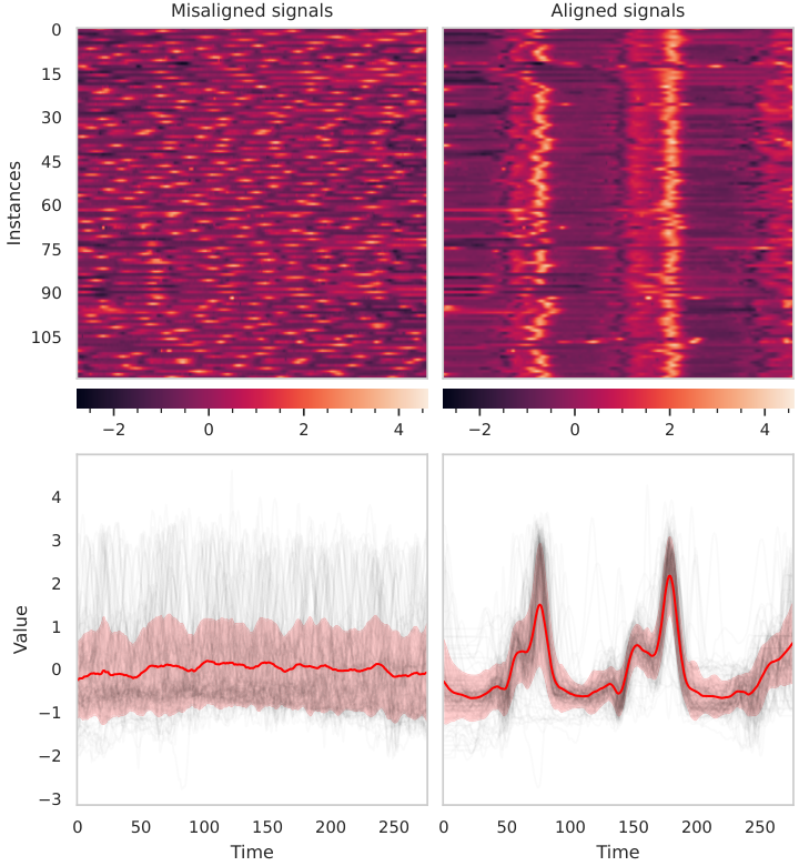
Results show that temporal misalignment strongly affects the Euclidean mean, and DBA usually reaches a local minimum. SoftDTW, DTAN and ResNet-TW show similar quantitative results. NCC test accuracy found that our method was better or no worse in 94% of the datasets compared with Euclidean, DBA (77%), SoftDTW (69%), DTAN (76%) and ResNet-TW (70%). Overall, our proposed TTN using DIFW beats all 5 comparing methods. The precise computation of the gradient of the transformation translates to an efficient search in the parameter space, which leads to faster and better solutions at convergence.
5 Conclusions
In this article a closed-form expression is presented for the gradient of CPA-based one-dimensional diffeomorphic transformations, providing efficiency, speed and precision. The proposed method was incorporated into a temporal transformer network that can both align pairwise sequential data and learn representative average sequences for multi-class joint alignment. Experiments performed on 84 datasets from the UCR archive show that our model achieves competitive performance in joint alignment and classification.
References
- Agrawal et al. (2019) Agrawal, A., Modi, A. N., Passos, A., Lavoie, A., Agarwal, A., Shankar, A., Ganichev, I., Levenberg, J., Hong, M., Monga, R., et al. Tensorflow eager: A multi-stage, python-embedded dsl for machine learning. arXiv preprint arXiv:1903.01855, 2019.
- Arsigny et al. (2006a) Arsigny, V., Commowick, O., Pennec, X., and Ayache, N. A log-euclidean framework for statistics on diffeomorphisms. Lecture Notes in Computer Science (including subseries Lecture Notes in Artificial Intelligence and Lecture Notes in Bioinformatics), 4190 LNCS:924–931, 2006a. ISSN 16113349.
- Arsigny et al. (2006b) Arsigny, V., Commowick, O., Pennec, X., and Ayache, N. A log-euclidean polyaffine framework for locally rigid or affine registration. Lecture Notes in Computer Science (including subseries Lecture Notes in Artificial Intelligence and Lecture Notes in Bioinformatics), 4057 LNCS:120–127, 2006b. ISSN 16113349. doi: 10.1007/11784012˙15.
- Beg et al. (2005) Beg, M. F., Miller, M. I., Trouvé, A., and Younes, L. Computing large deformation metric mappings via geodesic flows of diffeomorphisms. International Journal of Computer Vision, 61(2):139–157, 2005. ISSN 09205691. doi: 10.1023/B:VISI.0000043755.93987.aa.
- Blondel et al. (2021) Blondel, M., Mensch, A., and Vert, J.-P. Differentiable divergences between time series, 2021.
- Bradbury et al. (2018) Bradbury, J., Frostig, R., Hawkins, P., Johnson, M. J., Leary, C., Maclaurin, D., Necula, G., Paszke, A., VanderPlas, J., Wanderman-Milne, S., and Zhang, Q. JAX: composable transformations of Python+NumPy programs, 2018. URL http://github.com/google/jax.
- Chen et al. (2019) Chen, R. T. Q., Rubanova, Y., Bettencourt, J., and Duvenaud, D. Neural ordinary differential equations, 2019.
- Cuturi & Blondel (2017) Cuturi, M. and Blondel, M. Soft-dtw: a differentiable loss function for time-series. In International Conference on Machine Learning, pp. 894–903. PMLR, 2017.
- Dalca et al. (2018) Dalca, A. V., Balakrishnan, G., Guttag, J., and Sabuncu, M. R. Unsupervised learning for fast probabilistic diffeomorphic registration. In International Conference on Medical Image Computing and Computer-Assisted Intervention, pp. 729–738. Springer, 2018.
- Dau et al. (2019) Dau, H. A., Bagnall, A., Kamgar, K., Yeh, C.-C. M., Zhu, Y., Gharghabi, S., Ratanamahatana, C. A., and Keogh, E. The UCR Time Series Archive, 2019.
- Daulbaev et al. (2020) Daulbaev, T., Katrutsa, A., Markeeva, L., Gusak, J., Cichocki, A., and Oseledets, I. Interpolation technique to speed up gradients propagation in neural odes, 2020.
- Detlefsen (2018) Detlefsen, N. S. libcpab. https://github.com/SkafteNicki/libcpab, 2018.
- Detlefsen & Hauberg (2019) Detlefsen, N. S. and Hauberg, S. Explicit disentanglement of appearance and perspective in generative models. Advances in Neural Information Processing Systems, 32(NeurIPS), 2019. ISSN 10495258.
- Detlefsen et al. (2018) Detlefsen, N. S., Freifeld, O., and Hauberg, S. Deep Diffeomorphic Transformer Networks. Proceedings of the IEEE Computer Society Conference on Computer Vision and Pattern Recognition, pp. 4403–4412, 2018. ISSN 10636919. doi: 10.1109/CVPR.2018.00463.
- Duistermaat & Kolk (2000) Duistermaat, J. and Kolk, J. Lie groups and lie algebras. In Lie Groups, pp. 1–92. Springer, 2000.
- Freifeld (2018) Freifeld, O. Deriving the cpab derivative. Rn, 1:11, 2018.
- Freifeld et al. (2015) Freifeld, O., Hauberg, S., Batmanghelich, K., and Fisher, J. W. Highly-expressive spaces of well-behaved transformations: Keeping it simple. Proceedings of the IEEE International Conference on Computer Vision, 2015 Inter:2911–2919, 2015. ISSN 15505499. doi: 10.1109/ICCV.2015.333.
- Freifeld et al. (2017) Freifeld, O., Hauberg, S., Batmanghelich, K., and Fisher, J. W. Transformations Based on Continuous Piecewise-Affine Velocity Fields. IEEE Transactions on Pattern Analysis and Machine Intelligence, 39(12):2496–2509, 2017. ISSN 01628828. doi: 10.1109/TPAMI.2016.2646685.
- Fu et al. (2020) Fu, Y., Lei, Y., Wang, T., Curran, W. J., Liu, T., and Yang, X. Deep learning in medical image registration: a review. Physics in Medicine & Biology, 65(20):20TR01, 2020.
- Higham (2009) Higham, N. J. The scaling and squaring method for the matrix exponential revisited. SIAM Review, 51(4):747–764, 2009. ISSN 00361445. doi: 10.1137/090768539.
- Huang et al. (2021) Huang, H., Amor, B. B., Lin, X., Zhu, F., and Fang, Y. Residual Networks as Flows of Velocity Fields for Diffeomorphic Time Series Alignment. 2021. URL http://arxiv.org/abs/2106.11911.
- Innes (2018) Innes, M. Don’t unroll adjoint: Differentiating ssa-form programs. CoRR, abs/1810.07951, 2018. URL http://arxiv.org/abs/1810.07951.
- Jaderberg et al. (2015) Jaderberg, M., Simonyan, K., Zisserman, A., and Kavukcuoglu, K. Spatial transformer networks. Advances in Neural Information Processing Systems, 2015-Janua:2017–2025, 2015. ISSN 10495258.
- Kawano et al. (2020) Kawano, K., Kutsuna, T., and Koide, S. Neural time warping for multiple sequence alignment. In ICASSP 2020-2020 IEEE International Conference on Acoustics, Speech and Signal Processing (ICASSP), pp. 3837–3841. IEEE, 2020.
- Khorram et al. (2019) Khorram, S., McInnis, M. G., and Mower Provost, E. Trainable Time Warping: Aligning Time-series in the Continuous-time Domain. ICASSP, IEEE International Conference on Acoustics, Speech and Signal Processing - Proceedings, 2019-May:3502–3506, 2019. ISSN 15206149. doi: 10.1109/ICASSP.2019.8682322.
- Kingma & Ba (2014) Kingma, D. P. and Ba, J. Adam: A method for stochastic optimization. arXiv preprint arXiv:1412.6980, 2014.
- Lohit et al. (2019) Lohit, S., Wang, Q., and Turaga, P. Temporal transformer networks: Joint learning of invariant and discriminative time warping. Proceedings of the IEEE Computer Society Conference on Computer Vision and Pattern Recognition, 2019-June:12418–12427, 2019. ISSN 10636919. doi: 10.1109/CVPR.2019.01271.
- Ma et al. (2021) Ma, Y., Dixit, V., Innes, M., Guo, X., and Rackauckas, C. A comparison of automatic differentiation and continuous sensitivity analysis for derivatives of differential equation solutions, 2021.
- Moler & Van Loan (2003) Moler, C. and Van Loan, C. Nineteen dubious ways to compute the exponential of a matrix, twenty-five years later. SIAM Review, 45(1):3–49, 2003. ISSN 00361445. doi: 10.1137/S00361445024180.
- Moses & Churavy (2020) Moses, W. and Churavy, V. Instead of rewriting foreign code for machine learning, automatically synthesize fast gradients. In Larochelle, H., Ranzato, M., Hadsell, R., Balcan, M. F., and Lin, H. (eds.), Advances in Neural Information Processing Systems, volume 33, pp. 12472–12485. Curran Associates, Inc., 2020.
- Mumford & Desolneux (2010) Mumford, D. and Desolneux, A. Pattern theory: the stochastic analysis of real-world signals. CRC Press, 2010.
- Nunez & Joshi (2020) Nunez, E. and Joshi, S. H. Deep learning of warping functions for shape analysis. IEEE Computer Society Conference on Computer Vision and Pattern Recognition Workshops, 2020-June:3782–3790, 2020. ISSN 21607516. doi: 10.1109/CVPRW50498.2020.00441.
- Nunez et al. (2021) Nunez, E., Lizarraga, A., and Joshi, S. H. SrvfNet: A Generative Network for Unsupervised Multiple Diffeomorphic Shape Alignment. 2021. URL http://arxiv.org/abs/2104.13449.
- Oh et al. (2018) Oh, J., Wang, J., and Wiens, J. Learning to exploit invariances in clinical time-series data using sequence transformer networks. In Machine Learning for Healthcare Conference, pp. 332–347. PMLR, 2018.
- Paszke et al. (2019) Paszke, A., Gross, S., Massa, F., Lerer, A., Bradbury, J., Chanan, G., Killeen, T., Lin, Z., Gimelshein, N., Antiga, L., et al. Pytorch: An imperative style, high-performance deep learning library. Advances in neural information processing systems, 32:8026–8037, 2019.
- Petitjean et al. (2011) Petitjean, F., Ketterlin, A., and Gançarski, P. A global averaging method for dynamic time warping, with applications to clustering. Pattern Recognition, 44(3):678–693, 2011.
- Queiruga et al. (2020) Queiruga, A. F., Erichson, N. B., Taylor, D., and Mahoney, M. W. Continuous-in-depth neural networks, 2020.
- Rackauckas et al. (2019) Rackauckas, C., Innes, M., Ma, Y., Bettencourt, J., White, L., and Dixit, V. Diffeqflux.jl - a julia library for neural differential equations, 2019.
- Revels (2020) Revels, J. ReverseDiff.jl, 2020. Julia Package.
- Rivet & Cohen (2016) Rivet, B. and Cohen, J. E. Modeling time warping in tensor decomposition. In 2016 IEEE Sensor Array and Multichannel Signal Processing Workshop (SAM), pp. 1–5, 2016. doi: 10.1109/SAM.2016.7569733.
- Rousseau et al. (2019) Rousseau, F., Drumetz, L., Fablet, R., Rousseau, F., Drumetz, L., Fablet, R., and Networks, R. Residual Networks as Flows of Diffeomorphisms To cite this version : HAL Id : hal-01796729. 2019.
- Sakoe & Chiba (1978) Sakoe, H. and Chiba, S. Dynamic programming algorithm optimization for spoken word recognition. IEEE transactions on acoustics, speech, and signal processing, 26(1):43–49, 1978.
- Srivastava & Klassen (2016) Srivastava, A. and Klassen, E. P. Functional and shape data analysis, volume 1. Springer, 2016.
- Srivastava et al. (2011) Srivastava, A., Klassen, E., Joshi, S. H., and Jermyn, I. H. Shape analysis of elastic curves in euclidean spaces. IEEE Transactions on Pattern Analysis and Machine Intelligence, 33(7):1415–1428, 2011. ISSN 01628828. doi: 10.1109/TPAMI.2010.184.
- Van der Maaten & Hinton (2008) Van der Maaten, L. and Hinton, G. Visualizing data using t-sne. Journal of machine learning research, 9(11), 2008.
- van der Ouderaa et al. (2021) van der Ouderaa, T. F., Isgum, I., Veldhuis, W. B., Vos, B. D. D., and Moeskops, P. Diffeomorphic template transformers, 2021. URL https://openreview.net/forum?id=_sCOYXNwaI.
- Veeraraghavan et al. (2009) Veeraraghavan, A., Srivastava, A., Roy-Chowdhury, A. K., and Chellappa, R. Rate-invariant recognition of humans and their activities. IEEE Transactions on Image Processing, 18(6):1326–1339, 2009.
- Vercauteren et al. (2009) Vercauteren, T., Pennec, X., Perchant, A., and Ayache, N. Diffeomorphic demons: Efficient non-parametric image registration. NeuroImage, 45(1):S61–S72, 2009.
- Weber et al. (2019) Weber, R. S., Eyal, M., Detlefsen, N. S., Shriki, O., and Freifeld, O. Diffeomorphic temporal alignment nets. Advances in Neural Information Processing Systems, 32(NeurIPS), 2019. ISSN 10495258.
- Zhang & Sandu (2014) Zhang, H. and Sandu, A. Fatode: a library for forward, adjoint, and tangent linear integration of odes. SIAM Journal on Scientific Computing, 36(5):C504–C523, 2014.
- Zhou & De La Torre (2012) Zhou, F. and De La Torre, F. Generalized time warping for multi-modal alignment of human motion. Proceedings of the IEEE Computer Society Conference on Computer Vision and Pattern Recognition, pp. 1282–1289, 2012. ISSN 10636919. doi: 10.1109/CVPR.2012.6247812.
- Zhuang et al. (2020) Zhuang, J., Dvornek, N., Li, X., Tatikonda, S., Papademetris, X., and Duncan, J. Adaptive checkpoint adjoint method for gradient estimation in neural ode, 2020.
- Zhuang et al. (2021) Zhuang, J., Dvornek, N. C., Tatikonda, S., and Duncan, J. S. Mali: A memory efficient and reverse accurate integrator for neural odes, 2021.
Appendix A Velocity Continuity Constraints
Let’s consider three adjacent cells with affine transformations , and . The velocity field must be continuous. The velocity field is denoted as , since it depends on the affine tranformation . is continuous on every cell, because it is a linear function, but it is discontinuous on cell boundaries. Continuity of at implies one linear constraint on and . In the same way, continuity of at implies another linear constraint on and .
. In order to be continuous on points and , two linear constraints must be satisfied:
| (10) |
To place the linear constraints in matrix form, let’s recall the vectorize operation for this case:
| (11) |
Therefore,
| (12) |
Extending the continuity constraints to a tessellation with cells, the constraint matrix has dimensions , is and the null vector is . The number of shared vertices is .
Any matrix that satisfies will be continuous everywhere. The null space of coincides with the CPA vector-field space.
Appendix B Computing Infrastructures
We used the following computing infrastructure in our experiments: Intel(R) Core(TM) i7-6560U CPU @2.20GHz, 4 cores, 16gb RAM with an Nvidia Tesla P100 graphic card.
Appendix C Null Space of the Constraint Matrix
Four different methods have been implemented to obtain the null space of :
- 1.
SVD decomposition
- 2.
QR decomposition
- 3.
Reduced Row Echelon Form (RREF)
- 4.
Sparse form (SPARSE)
Given that the RREF and the Sparse basis can be computed efficiently in closed-form, the computation time of these null spaces is several orders of magnitude faster than SVD and QR Nonetheless, note that the null space only needs to be computed once, and as a result, this operation is not a critical step in the whole process to obtain the diffeomorphic trajectory.

Appendix D Integration Details
Given the initial value problem (IVT) defined by an ordinary differential equation (ODE) together with an initial condition:
| (13) |
D.1 Analytical Solution
To obtain the analytical solution we follow the separation of variables method, in which algebra allows one to rewrite the equation so that each of two variables occurs on a different side of the equation. We rearrange the ODE and integrate both sides:
| (14) |
| (15) | |||
| (16) | |||
| (17) |
The initial condition is then used to solve the unknown integration constant :
| (18) |
With that, we can obtain the closed-form expression for the IVP:
| (19) |
| (20) |
D.2 Matrix Form Solution
As an alternative, we can compute the IVT solution by transforming the system into matrix form and then using the matrix exponential operation. First, let’s rearrange the ODE into a matrix:
| (21) |
where is the affine vector, is the augmented affine matrix, and and are augmented vectors for and respectively.
The solution to the augmented ODE is given via the exponential matrix action: . The matrix exponential of a matrix can be mathematically defined by the Taylor series expansion, likewise to the exponential function :
| (22) |
In this case, . To calculate the matrix exponential of , we need to derive an expression for the infinite powers of . This can be obtained by generalizing the sequence of matrix products, or by using the Cayley Hamilton theorem.
a) If we try to generalize the sequence of matrix product:
(23)
(24)
(25)
(26)
(27) Then,
(28)
b) Rather, using the Cayley Hamilton theorem:
The characteristic polynomial of the matrix is given by:
The Cayley–Hamilton theorem claims that, if we define then . Hence, and as a consequence, . Now, using the exponential matrix expression we arrive at the same outcome as before:
(29)
Finally, from these two identical expressions, we can extract the same result obtained in the analytical solution:
| (30) |
| (31) |
Appendix E Comparing ODE Numerical and Closed-Form Methods for CPA Velocity Functions
In this article, we construct diffeomorphic curves by the integration of velocity functions. Specifically we work with continuous piecewise affine (CPA) velocity functions. The integral equation or the equivalent ODE can be solved numerically using any generic ODE solver.
In this sense, (Freifeld et al. 2015; Freifeld et al. 2017) proposed a specialized solver for integrating CPA fields which alternates between the analytic solution and a generic solver. This specialized solver is faster and more accurate than a generic solver since most of the trajectory is solved exactly, while the generic solver is only called in small portions. The two parameters used in (Freifeld et al. 2017), and imply two step sizes, one large used for exact updates, and one small, used for the generic-solver subroutine. By construction, the proposed closed-form solution is more accurate (exact solution) for both the ODE solution and for its derivative with respect to the velocity function parameters. We verified this empirically, comparing the specialized solver presented in (Freifeld et al. 2015; Freifeld et al. 2017) against the closed-form methods described in Sections 3.3 and 3.4. We compared the integration (and gradient) error averaged over random CPA velocity fields; i.e. we drew 100 CPA velocity functions from the prior (normal distribution of zero mean and unit standard deviation), , sampled uniformly 1000 points in , , and then computed the error:
| (32) |
The intention with this analysis was to study the number of numerical steps necessary to guarantee good enough integration and gradient estimations. The warping function is a bijective map from to . Figure 12 shows the precision obtained for different values of and . For instance, using the recommended values for and by the authors in (Freifeld et al. 2017) ( and ) we get a 5 decimals precision for the integration result but only 3 decimals for the gradient computation. Recall that Equation 32 computes the maximum absolute difference, and that the total error can be much higher over the entire gradient function. Lack of precision in the computation of transformation gradient translates to inefficient search in the parameter space, which leads to worse training processes and non-optimal solutions.


Appendix F Closed-Form Derivatives of w.r.t.
Let’s recall that the trajectory (the solution for the integral equation 1) is a composition of a finite number of solutions , as given by:
| (33) |
During the iterative process of integration, several cells are crossed, starting from at integration time , and finishing at at integration time . The integration time of the last cell can be calculated by subtracting from the initial integration time the accumulated boundary hitting times : . The final integration point is the boundary of the penultimate cell : . In case only one cell is visited, both time and space remain unchanged: and . Taking this into consideration, the trajectory can be calculated as follows:
| (34) |
In this section both the -dependent and are expressed as and to avoid overloading the notation. Therefore, the derivative can be calculated by going backwards in the integration direction. We are interested in the derivative of the trajectory w.r.t. the parameters . To obtain such gradient, we focus on the partial derivative w.r.t. one of the coefficients of , i.e., :
| (35) |
Let’s derive each of the terms of this derivative:
.
Notation. Recall the expression for from Section 3.2:
(36) Note that the slope and intercept are a linear combination of the orthogonal basis of the constraint matrix , with as coefficients.
(37) If we define one of the components from the orthogonal basis as:
(38) Then,
(39) And as a result,
(40) Thus, the slope and intercept ( parameters of the affine transformation) are denoted as follows:
(41)
F.1 Expression for
On the basis of the expression for ,
| (42) |
apply the chain-rule to obtain the derivative w.r.t :
| (43) |
Considering Equation 42 it is immediate to obtain the partial derivatives of and w.r.t :
| (44) |
| (45) |
Next, we find the derivative w.r.t and :
| (46) |
| (47) |
Finally, these expressions (Equations 44, 45, 46 and 47) are joined together into Equation 43:
| (48) |
F.2 Expression for
Starting from the expression for ,
| (49) |
we explicitly get the derivative w.r.t :
| (50) |
F.3 Expression for
After visiting cells, the integration time can be expressed as:
| (51) |
The derivative w.r.t. is obtained as follows:
| (52) |
where
| (53) |
and is the boundary for cell index . Now, apply the chain rule operation to the hitting time expression:
| (54) |
As it was previously derived in Section F.2, considering Equation 42 it is immediate to obtain the partial derivatives of and w.r.t :
| (55) |
| (56) |
Next, we develop the derivatives of w.r.t and :
| (57) |
| (58) |
Finally, these expressions (Equations 55, 56, 57 and 58) are joined together to obtain the derivative of w.r.t into Equation 54:
| (59) |
F.4 Expression for
After visiting cells, the integration point is the boundary point of the last visited cell. In case only one cell is visited, the integration point remains unchanged. In either case, does not depend on the parameters , thus
| (60) |
F.5 Final Expression for
Joining all the terms together and evaluating the derivative at and yields:
| (61) |
Appendix G Closed-Form Transformation when Slope
This special case ( leads to some indeterminations in the previous expressions for the integral (Equation 4) and derivative (Equation 5), consequently in this section we analyze and provide specific solutions. Note: infinitesimal equivalents of the exponential and natural logarithm functions: , if , and , if .
G.1 Integration when Slope
Recall the expression for from Section 3.2:
| (62) |
Estimate the limit of this expression when tends to zero:
| (63) |
| (64) |
Also, for the gradient computation it will be convenient to derive the expression for the hitting time of the boundary of :
| (65) |
| (66) |
| (67) |
G.2 Derivative when Slope
Note that the partial derivative w.r.t. one of the coefficients of , i.e., is expressed as:
| (68) |
To particularize this derivative to the special case , we first introduce the expressions obtained in Appendix F and then apply the limit when tends to zero.
G.2.1 Expression for when
| (69) |
| (70) |
G.2.2 Expression for when
If the partial derivative of w.r.t is given by:
| (71) |
then,
| (72) |
G.2.3 Expression for when
Recall that the partial derivative of the w.r.t depends on the previously hit boundaries:
| (73) |
| (74) |
Therefore,
| (75) |
| (76) |
G.2.4 Final Expression for when
Joining all the terms together and evaluating the derivative at and yields:
| (77) |
Appendix H Linear Interpolation Grid
Let be a discretized one-dimensional function defined by two arrays, i.e the input , and the output , such that . The differentiable time series sampler presented in the Temporal Transformer Network (TTN) is in charge of interpolating output values based on input values, i.e. get an estimate of the function value at using piecewise linear interpolation .
For a general irregular grid , is defined as follows:
| (78) |
where are known as the basis (hat functions), denoted as:
| (79) |
for , with the boundary ”half-hat” basis and .
In a regular grid every pair of values are separated by the same distance . In such case, the above expression for simplifies to:
| (80) |
The piecewise linear interpolation method is differentiable, which is a necessary condition to propagate the loss to the rest of the model. Thus, let’s compute the derivative of the piecewise linear interpolation function with respect to , and :
| (81) |
| (82) |
| (83) |
Self-composition
In order to apply the scaling-squaring approximate method we are interested in a special case of the piecewise linear interpolation in which the input is one of the output values , i.e. . In such case the derivative with respect to is extended as follows:
| (84) |
Appendix I Scaling-and-Squaring Integration Method
The scaling-and-squaring method needs to balance two factors to be competitive: the faster integration computation (scaling step) versus the extra time to self-compose the trajectory multiple times (squaring step). Figure 14 shows (top) the integration error (RMS) and (bottom) the computation time for different squaring iterations . Similarly, Figure 14 shows the error and the time for computing the derivative of the ODE solution for different scaling values . Under this setting, represents the parameter vector . Thus, a large value generates large deformations.
Executing more squaring iterations (large ) yields larger errors (both in the forward and backward operations). Even though the computation time increases for small deformations (positive slope for ) as the number of squaring iterations increases, experiments show that for large deformations computation speed can be gained at the expense of small integration errors. For example, in the backward operation with , takes around ms to compute if no scaling-and-squaring method is used. On the contrary, applying the scaling-and-squaring method 8 times (a reduction factor of ) reduces the computation time to around 2.5 ms (50% improvement), at the expense of 0.0035 RMS error in the gradient value. Therefore, this study shows that the scaling-and-squaring method can boost the speed performance for large deformations.
Appendix J UCR Archive (Dau et al. 2019) Dataset List
| Dataset | Train | Test | Length | Classes | Type |
|---|---|---|---|---|---|
| Adiac | 390 | 391 | 176 | 37 | Image |
| ArrowHead | 36 | 175 | 251 | 3 | Image |
| Beef | 30 | 30 | 470 | 5 | Spectro |
| BeetleFly | 20 | 20 | 512 | 2 | Image |
| BirdChicken | 20 | 20 | 512 | 2 | Image |
| Car | 60 | 60 | 577 | 4 | Sensor |
| CBF | 30 | 900 | 128 | 3 | Simulated |
| ChlorineConcentration | 467 | 3840 | 166 | 3 | Simulated |
| CinCECGTorso | 40 | 1380 | 1639 | 4 | ECG |
| Coffee | 28 | 28 | 286 | 2 | Spectro |
| Computers | 250 | 250 | 720 | 2 | Device |
| CricketX | 390 | 390 | 300 | 12 | Motion |
| CricketY | 390 | 390 | 300 | 12 | Motion |
| CricketZ | 390 | 390 | 300 | 12 | Motion |
| DiatomSizeReduction | 16 | 306 | 345 | 4 | Image |
| DistalPhalanxOutlineAgeGroup | 400 | 139 | 80 | 3 | Image |
| DistalPhalanxOutlineCorrect | 600 | 276 | 80 | 2 | Image |
| DistalPhalanxTW | 400 | 139 | 80 | 6 | Image |
| Earthquakes | 322 | 139 | 512 | 2 | Sensor |
| ECG200 | 100 | 100 | 96 | 2 | ECG |
| ECG5000 | 500 | 4500 | 140 | 5 | ECG |
| ECGFiveDays | 23 | 861 | 136 | 2 | ECG |
| ElectricDevices | 8926 | 7711 | 96 | 7 | Device |
| FaceAll | 560 | 1690 | 131 | 14 | Image |
| FaceFour | 24 | 88 | 350 | 4 | Image |
| FacesUCR | 200 | 2050 | 131 | 14 | Image |
| FiftyWords | 450 | 455 | 270 | 50 | Image |
| Fish | 175 | 175 | 463 | 7 | Image |
| FordA | 3601 | 1320 | 500 | 2 | Sensor |
| FordB | 3636 | 810 | 500 | 2 | Sensor |
| GunPoint | 50 | 150 | 150 | 2 | Motion |
| Ham | 109 | 105 | 431 | 2 | Spectro |
| HandOutlines | 1000 | 370 | 2709 | 2 | Image |
| Haptics | 155 | 308 | 1092 | 5 | Motion |
| Herring | 64 | 64 | 512 | 2 | Image |
| InlineSkate | 100 | 550 | 1882 | 7 | Motion |
| InsectWingbeatSound | 220 | 1980 | 256 | 11 | Sensor |
| ItalyPowerDemand | 67 | 1029 | 24 | 2 | Sensor |
| LargeKitchenAppliances | 375 | 375 | 720 | 3 | Device |
| Lightning2 | 60 | 61 | 637 | 2 | Sensor |
| Lightning7 | 70 | 73 | 319 | 7 | Sensor |
| Mallat | 55 | 2345 | 1024 | 8 | Simulated |
| Meat | 60 | 60 | 448 | 3 | Spectro |
| MedicalImages | 381 | 760 | 99 | 10 | Image |
| MiddlePhalanxOutlineAgeGroup | 400 | 154 | 80 | 3 | Image |
| MiddlePhalanxOutlineCorrect | 600 | 291 | 80 | 2 | Image |
| MiddlePhalanxTW | 399 | 154 | 80 | 6 | Image |
| MoteStrain | 20 | 1252 | 84 | 2 | Sensor |
| NonInvasiveFetalECGThorax1 | 1800 | 1965 | 750 | 42 | ECG |
| NonInvasiveFetalECGThorax2 | 1800 | 1965 | 750 | 42 | ECG |
| OliveOil | 30 | 30 | 570 | 4 | Spectro |
| OSULeaf | 200 | 242 | 427 | 6 | Image |
| PhalangesOutlinesCorrect | 1800 | 858 | 80 | 2 | Image |
| Phoneme | 214 | 1896 | 1024 | 39 | Sensor |
| Plane | 105 | 105 | 144 | 7 | Sensor |
| ProximalPhalanxOutlineAgeGroup | 400 | 205 | 80 | 3 | Image |
| ProximalPhalanxOutlineCorrect | 600 | 291 | 80 | 2 | Image |
| ProximalPhalanxTW | 400 | 205 | 80 | 6 | Image |
| RefrigerationDevices | 375 | 375 | 720 | 3 | Device |
| ScreenType | 375 | 375 | 720 | 3 | Device |
| ShapeletSim | 20 | 180 | 500 | 2 | Simulated |
| ShapesAll | 600 | 600 | 512 | 60 | Image |
| SmallKitchenAppliances | 375 | 375 | 720 | 3 | Device |
| SonyAIBORobotSurface1 | 20 | 601 | 70 | 2 | Sensor |
| SonyAIBORobotSurface2 | 27 | 953 | 65 | 2 | Sensor |
| Strawberry | 613 | 370 | 235 | 2 | Spectro |
| SwedishLeaf | 500 | 625 | 128 | 15 | Image |
| Symbols | 25 | 995 | 398 | 6 | Image |
| SyntheticControl | 300 | 300 | 60 | 6 | Simulated |
| ToeSegmentation1 | 40 | 228 | 277 | 2 | Motion |
| ToeSegmentation2 | 36 | 130 | 343 | 2 | Motion |
| Trace | 100 | 100 | 275 | 4 | Sensor |
| TwoLeadECG | 23 | 1139 | 82 | 2 | ECG |
| TwoPatterns | 1000 | 4000 | 128 | 4 | Simulated |
| UWaveGestureLibraryAll | 896 | 3582 | 945 | 8 | Motion |
| UWaveGestureLibraryX | 896 | 3582 | 315 | 8 | Motion |
| UWaveGestureLibraryY | 896 | 3582 | 315 | 8 | Motion |
| UWaveGestureLibraryZ | 896 | 3582 | 315 | 8 | Motion |
| Wafer | 1000 | 6164 | 152 | 2 | Sensor |
| Wine | 57 | 54 | 234 | 2 | Spectro |
| WordSynonyms | 267 | 638 | 270 | 25 | Image |
| Worms | 181 | 77 | 900 | 5 | Motion |
| WormsTwoClass | 181 | 77 | 900 | 2 | Motion |
| Yoga | 300 | 3000 | 426 | 2 | Image |
Appendix K Additional Alignment Results of Test Data
In this section, we provide more qualitative results of joint alignment of test data in different datasets from the UCR archive (Dau et al. 2019).


Figure 17 shows a t-SNE (Van der Maaten & Hinton 2008) visualization of the original and aligned data of the 11-class FacesUCR dataset. This illustrates how our TTN indeed decreases intra-class variance while increasing inter-class one, thus improving the performance of classification.
Appendix L Nearest Centroid Classification (NCC) Results
In this section, we show detailed quantitative results of the NCC experiment on UCR archive (Dau et al. 2019) in Figures 19, 20, 2 and 3. We compare our Temporal Transformer Network with Euclidean average (as a baseline), DTW Barycenter Averaging (DBA) (Petitjean et al. 2011), SoftDTW (Cuturi & Blondel 2017), DTAN (Weber et al. 2019) and ResNet-TW (Huang et al. 2021).


| Type (count) | Euclidean | DBA | SoftDTW | DTAN | ResNet-TW | Ours |
|---|---|---|---|---|---|---|
| Device (6) | 0.425781 | 0.584495 | 0.591291 | 0.523803 | 0.534700 | 0.540954 |
| ECG (7) | 0.687460 | 0.706706 | 0.705433 | 0.855727 | 0.814560 | 0.918076 |
| Image (29) | 0.625407 | 0.660084 | 0.686681 | 0.719903 | 0.739120 | 0.767902 |
| Motion (14) | 0.476806 | 0.577721 | 0.603160 | 0.579338 | 0.561593 | 0.609039 |
| Sensor (15) | 0.660346 | 0.651705 | 0.693455 | 0.749147 | 0.772336 | 0.783508 |
| Simulated (6) | 0.657427 | 0.786523 | 0.805312 | 0.710171 | 0.734658 | 0.770062 |
| Spectro (7) | 0.754846 | 0.700941 | 0.745851 | 0.805897 | 0.791203 | 0.866869 |
| Total (84) | 0.610865 | 0.655783 | 0.682124 | 0.705480 | 0.711170 | 0.748917 |
| Dataset | Euclidean | DBA | SoftDTW | DTAN | ResNet-TW | Ours |
|---|---|---|---|---|---|---|
| Adiac | 0.549872 | 0.462916 | 0.501279 | 0.695652 | 0.698210 | 0.718670 |
| ArrowHead | 0.611429 | 0.474286 | 0.520000 | 0.748571 | 0.754286 | 0.725714 |
| Beef | 0.533333 | 0.400000 | 0.566667 | 0.633333 | 0.633333 | 0.700000 |
| BeetleFly | 0.850000 | 0.900000 | 0.850000 | 0.800000 | 0.800000 | 0.950000 |
| BirdChicken | 0.550000 | 0.600000 | 0.700000 | 0.800000 | 0.950000 | 0.950000 |
| Car | 0.616667 | 0.633333 | 0.683333 | 0.816667 | 1.000000 | 0.988889 |
| CBF | 0.763333 | 0.965556 | 0.971111 | 0.914444 | 0.850000 | 0.982222 |
| ChlorineConcentration | 0.333073 | 0.323698 | 0.348177 | 0.333073 | 0.351823 | 0.396615 |
| CinCECGTorso | 0.385507 | 0.445652 | 0.398551 | 0.615942 | 0.542754 | 0.740580 |
| Coffee | 0.964286 | 0.964286 | 0.964286 | 1.000000 | 0.964290 | 1.000000 |
| Computers | 0.416000 | 0.616000 | 0.640000 | 0.592000 | 0.676000 | 0.616000 |
| CricketX | 0.238462 | 0.574359 | 0.602564 | 0.423077 | 0.341026 | 0.428205 |
| CricketY | 0.348718 | 0.541026 | 0.571795 | 0.541026 | 0.415385 | 0.512821 |
| CricketZ | 0.305128 | 0.605128 | 0.615385 | 0.420513 | 0.333333 | 0.451282 |
| DiatomSizeReduction | 0.957516 | 0.950980 | 0.950980 | 0.970588 | 0.973856 | 0.983660 |
| DistalPhalanxOutlineAgeGroup | 0.817500 | 0.840000 | 0.850000 | 0.847500 | 0.862500 | 0.748201 |
| DistalPhalanxOutlineCorrect | 0.471667 | 0.488333 | 0.490000 | 0.471667 | 0.505000 | 0.775362 |
| DistalPhalanxTW | 0.747500 | 0.755000 | 0.760000 | 0.780000 | 0.797500 | 0.683453 |
| Earthquakes | 0.754658 | 0.574534 | 0.822981 | 0.773292 | 0.973287 | 0.820000 |
| ECG200 | 0.750000 | 0.720000 | 0.730000 | 0.790000 | 0.795031 | 0.913778 |
| ECG5000 | 0.860444 | 0.834667 | 0.853778 | 0.891333 | 0.800000 | 0.998839 |
| ECGFiveDays | 0.689895 | 0.658537 | 0.670151 | 0.977933 | 0.931556 | 0.993031 |
| ElectricDevices | 0.482687 | 0.538970 | 0.539748 | 0.534820 | 0.518869 | 0.573726 |
| FaceAll | 0.491716 | 0.796450 | 0.827811 | 0.804734 | 0.840909 | 0.856213 |
| FaceFour | 0.840909 | 0.852273 | 0.852273 | 0.829545 | 0.855122 | 0.920455 |
| FacesUCR | 0.539512 | 0.774634 | 0.812683 | 0.857073 | 0.857143 | 0.800976 |
| FiftyWords | 0.516484 | 0.615385 | 0.615385 | 0.652747 | 0.516484 | 0.630769 |
| Fish | 0.560000 | 0.651429 | 0.697143 | 0.902857 | 0.902857 | 0.914286 |
| FordA | 0.495973 | 0.549570 | 0.552902 | 0.604832 | 0.568176 | 0.652273 |
| FordB | 0.499725 | 0.568482 | 0.591309 | 0.579758 | 0.566282 | 0.545679 |
| GunPoint | 0.753333 | 0.700000 | 0.733333 | 0.880000 | 0.806667 | 0.846667 |
| Ham | 0.761905 | 0.723810 | 0.733333 | 0.790476 | 0.761905 | 0.809524 |
| HandOutlines | 0.818000 | 0.804000 | 0.812000 | 0.850000 | 0.835000 | 0.908108 |
| Haptics | 0.392857 | 0.350649 | 0.373377 | 0.457792 | 0.464286 | 0.487013 |
| Herring | 0.546875 | 0.546875 | 0.609375 | 0.703125 | 0.765625 | 0.781250 |
| InlineSkate | 0.192727 | 0.232727 | 0.252727 | 0.260000 | 0.243636 | 0.287273 |
| InsectWingbeatSound | 0.601010 | 0.289394 | 0.328283 | 0.587374 | 0.570707 | 0.606566 |
| ItalyPowerDemand | 0.918367 | 0.730807 | 0.750243 | 0.962099 | 0.965015 | 0.966958 |
| LargeKitchenAppliances | 0.440000 | 0.728000 | 0.733333 | 0.482667 | 0.501333 | 0.517333 |
| Lightning2 | 0.688525 | 0.639344 | 0.622951 | 0.721311 | 0.754098 | 0.737705 |
| Lightning7 | 0.589041 | 0.698630 | 0.726027 | 0.712329 | 0.684932 | 0.726027 |
| Mallat | 0.966738 | 0.952665 | 0.953945 | 0.968870 | 0.966738 | 0.973561 |
| Meat | 0.933333 | 0.916667 | 0.933333 | 0.933333 | 0.933333 | 0.933333 |
| MedicalImages | 0.385526 | 0.436842 | 0.461842 | 0.468421 | 0.473684 | 0.482895 |
| MiddlePhalanxOutlineAgeGroup | 0.732500 | 0.712500 | 0.795000 | 0.737500 | 0.752500 | 0.636364 |
| MiddlePhalanxOutlineCorrect | 0.551667 | 0.483333 | 0.495000 | 0.543333 | 0.531667 | 0.697595 |
| MiddlePhalanxTW | 0.591479 | 0.556391 | 0.581454 | 0.596491 | 0.634085 | 0.538961 |
| MoteStrain | 0.861022 | 0.826677 | 0.843450 | 0.904153 | 0.912939 | 0.874601 |
| NonInvasiveFetalECGThorax1 | 0.769466 | 0.712977 | 0.710941 | 0.853435 | 0.838677 | 0.874300 |
| NonInvasiveFetalECGThorax2 | 0.802036 | 0.763868 | 0.773028 | 0.905344 | 0.838680 | 0.916539 |
| OliveOil | 0.866667 | 0.766667 | 0.800000 | 0.866667 | 0.866667 | 0.900000 |
| OSULeaf | 0.359504 | 0.438017 | 0.475207 | 0.462810 | 0.458678 | 0.933333 |
| PhalangesOutlinesCorrect | 0.625874 | 0.632867 | 0.637529 | 0.642191 | 0.663170 | 0.675991 |
| Phoneme | 0.078586 | 0.182489 | 0.204641 | 0.101793 | 0.116561 | 0.100738 |
| Plane | 0.961905 | 1.000000 | 0.990476 | 1.000000 | 1.000000 | 1.000000 |
| ProximalPhalanxOutlineAgeGroup | 0.819512 | 0.843902 | 0.853659 | 0.853659 | 0.873171 | 0.873171 |
| ProximalPhalanxOutlineCorrect | 0.646048 | 0.649485 | 0.725086 | 0.642612 | 0.687285 | 0.725086 |
| ProximalPhalanxTW | 0.707500 | 0.735000 | 0.747500 | 0.817500 | 0.822500 | 0.790244 |
| RefrigerationDevices | 0.354667 | 0.584000 | 0.586667 | 0.466667 | 0.482667 | 0.485333 |
| ScreenType | 0.442667 | 0.378667 | 0.389333 | 0.445333 | 0.469333 | 0.461333 |
| ShapeletSim | 0.500000 | 0.522222 | 0.588889 | 0.538889 | 0.588889 | 0.572222 |
| ShapesAll | 0.513333 | 0.603333 | 0.628333 | 0.628333 | 0.681667 | 0.643333 |
| SmallKitchenAppliances | 0.418667 | 0.661333 | 0.658667 | 0.621333 | 0.560000 | 0.592000 |
| SonyAIBORobotSurface1 | 0.811980 | 0.835275 | 0.893511 | 0.893511 | 0.860233 | 0.891847 |
| SonyAIBORobotSurface2 | 0.793284 | 0.766002 | 0.772298 | 0.811123 | 0.830010 | 0.875131 |
| Strawberry | 0.668842 | 0.616639 | 0.649266 | 0.843393 | 0.786297 | 0.891892 |
| SwedishLeaf | 0.702400 | 0.681600 | 0.723200 | 0.806400 | 0.836800 | 0.857600 |
| Symbols | 0.864322 | 0.954774 | 0.954774 | 0.857286 | 0.906533 | 0.911558 |
| SyntheticControl | 0.916667 | 0.980000 | 0.980000 | 0.950000 | 0.950000 | 0.980000 |
| ToeSegmentation1 | 0.574561 | 0.614035 | 0.671053 | 0.640351 | 0.653509 | 0.793860 |
| ToeSegmentation2 | 0.546154 | 0.838462 | 0.853846 | 0.753846 | 0.746154 | 0.784615 |
| Trace | 0.580000 | 0.970000 | 0.970000 | 0.780000 | 0.800000 | 0.980000 |
| TwoLeadECG | 0.554873 | 0.811238 | 0.801580 | 0.956102 | 0.955224 | 0.989464 |
| TwoPatterns | 0.464750 | 0.975000 | 0.989750 | 0.555750 | 0.700500 | 0.715750 |
| UWaveGestureLibraryAll | 0.849525 | 0.831937 | 0.833613 | 0.920715 | 0.911502 | 0.943886 |
| UWaveGestureLibraryX | 0.631212 | 0.676438 | 0.706868 | 0.681184 | 0.721943 | 0.710497 |
| UWaveGestureLibraryY | 0.548297 | 0.525405 | 0.564768 | 0.611669 | 0.617253 | 0.641262 |
| UWaveGestureLibraryZ | 0.537409 | 0.592406 | 0.604132 | 0.642099 | 0.646287 | 0.652150 |
| Wafer | 0.654445 | 0.511032 | 0.649416 | 0.988968 | 0.982803 | 0.986210 |
| Wine | 0.555556 | 0.518519 | 0.574074 | 0.574074 | 0.592593 | 0.833333 |
| WordSynonyms | 0.271160 | 0.344828 | 0.412226 | 0.474922 | 0.501567 | 0.474922 |
| Worms | 0.215470 | 0.414365 | 0.408840 | 0.259669 | 0.342541 | 0.337662 |
| WormsTwoClass | 0.541436 | 0.591160 | 0.651934 | 0.618785 | 0.618785 | 0.649351 |
| Yoga | 0.497000 | 0.557000 | 0.574000 | 0.631667 | 0.696667 | 0.681000 |
| Average accuracy | 0.610865 | 0.655783 | 0.682124 | 0.705480 | 0.711170 | 0.748917 |
| Average arithmetic ranking | 4.964 | 4.488 | 3.297 | 2.988 | 2.666 | 1.940 |
| Average geometric ranking | 4.760 | 4.077 | 2.816 | 2.730 | 2.299 | 1.589 |
| Winning times | 1 | 5 | 18 | 7 | 21 | 49 |
L.1 Hyperparameter Grid Search
For each of the UCR datasets, we trained our TTN for joint alignment as in (Weber et al. 2019), where , , , the number of transformer layers , scaling-and-squaring iterations and the option to apply the zero-boundary constraint. The full table of results is available in the Supplementary Materials, and was not included in the manuscript due to the large number of experiments for the 84 UCR datasets.
In total, different hyperparameter configurations were tested. To provide a summary of these experiments, we first gathered the hyperparameters that yield optimal (maximum) NCC test accuracy for each UCR dataset. Then we counted how many times each parameter value appears in the optimal NCC accuracy configuration for each of the 84 UCR datasets. Figure 21 shows the winning percentage of each hyperparameter value. For example, a tessellation size appears in of the winning parameter combinations among 84 datasets, while and get reduced to in respectively. The scaling-and-squaring method appears to be preferable based on the results, with of the datasets using 8 iterations of the method.
L.2 Ablation Study on Model Expressivity
Regarding the expressivity of the proposed model, it is worth noting that the fineness of the partition in CPA velocity functions controls the trade-off between expressiveness and computational complexity. An ablation study is presented in this section to investigate how partition fineness control affects such balance. We computed the training time and the model accuracy for different values of the tessellation size .
Figure 22 and Table 4 show the results from the ablation study in terms of model accuracy and compute time for all 84 UCR datasets and for different values of . Results show that increasing lead to longer training times, and large values can hinder accuracy performance. For instance, on average, going from 4 to 16 cells increments the training time by 1.5% and increments the NCC accuracy by 0.6962%. However, going from 16 to 32 cells increments the training time by 1.8% but reduces the NCC accuracy by 0.0905%.
|
| |||||
|---|---|---|---|---|---|---|
| 4 16 | 1.5% | 0.69% | ||||
| 16 32 | 1.8% | 0.09% | ||||
| 32 64 | 5.5% | 0.20% | ||||
| 64 128 | 16.3% | 0.24% | ||||
| 128 256 | 25.0% | 0.48% |
L.3 The Texas Sharpshooter Fallacy
The Texas Sharpshooter Fallacy is a common logic error that occurs when comparing methods across multiple datasets. In fact, it is not sufficient to have a method that can be more accurate on some datasets unless one can predict on which datasets it will be more accurate. Therefore, in this section we test whether the expected accuracy gain over another competing method coincides with the actual accuracy gain. The expected accuracy gain and the actual accuracy gain are defined by Equation 85 and Equation 86, respectively. An expected accuracy gain larger than one indicates that we predict our method will perform better, while an actual accuracy gain larger than one indicates that our method indeed performs better.
| (85) |
| (86) |
As shown in Figure 23, Texas sharpshooter plot is a convenient tool to visualize the comparison between the expected accuracy gain and the actual accuracy gain on multiple datasets. Each point represents a dataset which falls into one of the following four possibilities:
- •
TP (True Positive): we predicted that our method would increase accuracy, and it did. This is the most beneficial situation and the majority of points fall into this region.
- •
TN (True Negative): we predicted that our method would decrease accuracy, and it did. This is not truly a bad region since knowing ahead of time that a method will do worse allows choosing another method to avoid the loss of accuracy.
- •
FN (False Negative): we predicted that our method would decrease accuracy but it actually increased. This is also not a bad case even though we might miss the opportunity to improve.
- •
FP (False Positive): we predicted our method would increase accuracy and it did not. Truly the painful region to be, but fortunately not many points fall into it.
L.4 Correlation With Dataset Size
Finally, we analyze the correlation between the expected accuracy gain and the dataset size. For each competing method, we analyze whether more data availability translates into larger accuracy gains. As visualized in Figure 24, there is a lack of correlation between data availability and accuracy improvement across the five competing methods.