Three-Dimensional Alignment of Density Maps in Cryo-Electron Microscopy
Abstract
A common task in cryo-electron microscopy (cryo-EM) data processing is to compare three-dimensional density maps of macromolecules. In this paper, we propose an algorithm for aligning three-dimensional density maps that exploits common lines between projection images of the maps. The algorithm is fully automatic and handles rotations, reflections (handedness), and translations between the maps. In addition, the algorithm is applicable to any type of molecular symmetry without requiring any information regarding the symmetry of the maps. We evaluate our alignment algorithm on publicly available density maps, demonstrating its accuracy and efficiency. The algorithm is available at https://github.com/ShkolniskyLab/emalign.
1 Introduction
Single particle cryo-electron microscopy (cryo-EM) is a method to determine the three-dimensional structure of biological macromolecules from their two-dimensional projection images acquired by an electron microscope [1]. In this method, a sample of identical copies of the investigated molecule is quickly frozen in a thin layer of ice, where each copy is frozen at an unknown random orientation. The frozen sample is imaged by an electron microscope, resulting in two-dimensional images, where each image is a tomographic projection of one of the randomly oriented copies in the ice layer. The goal of single particle cryo-EM is to determine the three-dimensional structure of the molecule from the acquired two-dimensional images. A common task in cryo-EM data processing is to compare two density maps of the same molecule. This is required, for example, for estimating the resolution of the maps, evaluating their Fourier shell correlation curve [2], or to analyze their different conformations. All these tasks require to first align two density maps, that is, to orient them in the same way in a common coordinate system. Due to the nature of the cryo-EM imaging process, the two density maps may differ not only in their three-dimensional orientation (that is, their “rotation”), but may also have different handedness (namely, reflected relative to each other), and may be centered differently with respect to a common coordinate system.
In this paper, we propose an algorithm for aligning two density maps, which is fully automatic and can handle rotations, translations, and reflections between the maps. The algorithm requires as an input only the two density maps. In particular, it does not assume knowledge of any other information such as the symmetry of the maps.
Formally, let and be two volumes such that
| (1) |
where , and ( is the group of all orthogonal transformations of the three-dimensional space, namely, rotations and reflections). The alignment problem is to estimate and given and . The matrix is known as the orientation parameter, and the vector as the translation parameter. In practice, we only get samples of and , arranged as three-dimensional arrays of size , where is the resolution of sampling. In cryo-EM, and represent two reconstructions of the same underlying molecule that we would like to compare (such as two half maps from a refinement process). In principle, it is possible to approximate the solution to the alignment problem using exhaustive search, by generating a set of candidate pairs , where and , and finding the pair which “best aligns” to in some chosen metric. The purpose of the alignment algorithm presented in this paper is to estimate the optimal alignment parameters in a fast and accurate way.
The paper is organized as follows. In Section 2, we review existing alignment algorithms. In Section 3, we give a high level simplified description of our algorithm. A detailed description is then given in Section 4. This description relies of a method for aligning a single projection image against a volume, a procedure which is described in Section 5. In Section 6, we discuss implementation considerations of the algorithm, and analyze its complexity. An optional procedure for refining the estimated alignment parameters in described in Section 7. In Section 8, we demonstrate numerically the properties and performance of our algorithm. Finally, in Section 9, we discuss the properties and advantages of our algorithm.
2 Existing methods
There exist several methods for three-dimensional alignment of molecular volumes. The Chimera software [3] offers a semi-automatic alignment method which requires the user to approximately align the volumes manually, and then refines this alignment using an optimization procedure. This means that a sufficiently accurate initial approximation for the alignment is required. Achieving this initial approximate alignment manually naturally takes time and effort, yet it is crucial for the success of Chimera’s alignment algorithm. The alignment procedure implemented by Chimera maximizes the correlation or overlap function between the two volumes by using a steepest descent optimization. The iterations of this optimization stop after reaching convergence or after 2,000 steps.
Another alignment method is the projection based volume alignment algorithm (PBVA) [4]. This method aligns a target volume to a reference volume by aligning multiple projections of the reference volume to the target volume whose orientation is unknown. The PBVA algorithm is based on finding two identical projections, a projection from the reference volume and a projection from the target volume as follows. The reference volume is projected at some known Euler angles, resulting in a projection , and the matching projection is found by maximizing the cross-correlation function between and a set of projections representing the possible projections of the target volume. The cross-correlation function is of five parameters – three Euler angles and two translation parameters in the plane of the projection [5]. Finally, the rotation between the volumes is estimated from the relation between the Euler angles corresponding to the projections and . After estimating the rotation between the volumes, the translation between them is found using projection images from the target volume. The translation between the volumes is estimated by least-squares regression using the two translation parameters of each projection from the target volume, where a minimum of two projections is required for calculating the three-dimensional translation vector. Using multiple projection images to estimate the translation between the volumes makes the alignment more robust.
The Xmipp software package [6] also offers a three-dimensional alignment algorithm. It is based on expanding the two volumes using spherical harmonics followed by computing the cross-correlation function between the two spherical harmonics expansions representing the volumes [7]. The process of expanding a volume into spherical harmonics is called the Spherical Fourier Transform (SFT) of the volume, where like the FFT algorithm, there exists an efficient algorithm for calculating the SFT [7]. The process of calculating the cross-correlation function between the two spherical harmonics expansions of the volumes and estimating the rotation between the two volumes is implemented by a fast rotational matching (FRM) algorithm [8]. After estimating the rotation between the two volumes, the translation between them is found by using the phase correlation algorithm [9].
Finally, the EMAN2 software package [10] offers two three-dimensional alignment algorithms. In the first algorithm (implemented by the program e2align3d, now mostly obsolete), the rotation between the volumes is estimated using an exhaustive search for the three Euler angles of the rotation. First, the algorithm generates a set of candidate Euler angles with large angular increments. Then, the algorithm iteratively decreases the angular increments in the set of candidates in order to refine the resolution of the angular search [11]. A much faster tree-based algorithm is implemented in the program e2proc3d. This method performs three-dimensional rotational and translational alignment using a hierarchical method with gradually decreasing downsampling in Fourier space. In Section 8, we compare our algorithm to this latter algorithm, as well as to the fast rotational matching algorithm implemented by Xmipp.
3 Outline of the approach
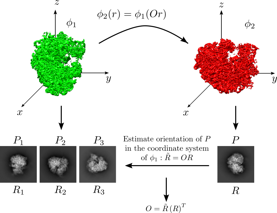
We are given two volumes and satisfying (1). For simplicity, we assume for now that the volumes have no symmetry, and are related by rotation only (no translation nor reflection). We generate a projection image from , denoted , corresponding to an orientation given by a rotation matrix . Since and are the same volume up to rotation, we can orient relative to , that is, we can find the rotation such that projecting in the orientation determined by results in the image . As we show below, it holds that , where is the transformation from (1). Since and are known, we can estimate as .
In practice, it may be that is not determined uniquely by , as for example, a volume may have two very similar views even if it is not symmetric. Moreover, the volumes to align are discretized and sometimes noisy, which introduces inaccuracies into the estimation of . Thus, to estimate more robustly, instead of using a single image , we generate from multiple images with orientations , align each to as above, resulting in estimates for given by , and then estimate from all simultaneously by solving
where is the Frobenius matrix norm. In Section 4, we give an explicit solution for the latter optimization problem.
The key of the above procedure is estimating the orientation of a projection image of in the coordinate system of . This is done by inspecting a large enough set of candidate rotations, and finding the rotation for which the induced common lines between (when assuming its orientation is ) and a set of projections generated from best agree. As inspecting each candidate rotation involves only one-dimensional operations (even if the input volumes are centered differently), it is very fast and highly parallelizable. Thus, this somewhat brute-force approach is applicable to very large sets of candidate rotations (several thousands, for accurate alignment) and still results in a fast algorithm. We discuss below the complexity and advantages of this approach. We summarize the outline of our approach in Fig. 1, and describe it in detail in Sections 4 and 5.
In the above approach, we assume that is a rotation. However, and may have a different handedness, and so may include a reflection. The above approach can obviously be used to resolve the handedness by aligning to and to a reflected copy of , and determining whether a reflection is needed using some quality score of the alignment parameters (e.g., the correlation between the aligned volumes). However, as we show below, in our method, there is no need to actually align to a reflected copy of , saving roughly half of the computations (those required to actually align to a reflected copy of ), as explained in Section 4.
We next explain in detail the various steps of our algorithm, including handling translations, reflections, and symmetry in the volumes.
4 Estimating the alignment parameters
Consider two volumes and , where one volume is a rotated copy of the other (assuming for now no reflection nor translation between the volumes), namely (see (1))
| (2) |
where is an unknown rotation matrix. Our goal is to find an estimate for .
In case where and exhibit symmetry, the solution for is not unique. To be concrete, we denote by the group of all rotation matrices. A group is a symmetry group of a volume , if for all it holds that
| (3) |
In other words, a symmetry group of a volume is a group of rotations under which the volume is invariant (see [12] for more details). If we denote the symmetry group of by and define , then, from (2) and (3), we get for any symmetry element
| (4) |
Comparing the latter with (2), we conclude that the solution for is not unique, and we thus replace the goal of finding by finding any for some arbitrary element of the symmetry group.
Note that we assume that is a rotation, namely that and are related by rotation without reflection. The case where is a reflection will be considered below. Let be a projection image generated from using a rotation , that is
| (5) |
where , , are the columns of the matrix and . From (2), we have that
| (6) |
Thus, using (5), we have
| (7) |
Equation (7) implies that if has orientation with respect to , then it has orientation with respect to . In Section 5, we describe how to estimate given and , namely, how to estimate a rotation that satisfies . If the volume is symmetric with symmetry group , then (as shown above) the rotation is equivalent to the rotation for any , and moreover, the two rotations cannot be distinguished. Thus, we conclude that
for some unknown . Using the latter equation, we can estimate as
| (8) |
Note that in the latter equation is known, can estimated using the algorithm in Section 5 below, and can be arbitrary. Thus, (8) provides a means for estimating .
However, to estimate more robustly, we use multiple projections generated from . Let be random rotations, and let be the corresponding projections generated from according to (5). Using the procedure described above, we estimate for each a rotation that satisfies for some unknown . Thus, as in (8), we can estimate using any by
| (9) |
Contrary to (8), if we want the right hand side of (9) to result in the same for all , then cannot be arbitrary. In order to estimate , we therefore need to find , , and combine all estimates for given in (9) into a single estimate.
To that end, define
| (10) |
and look at the matrix of size whose block of size is given by (see (9) and (10))
| (11) | ||||
By a direct calculation, we get that the matrix of size
| (12) |
where is an arbitrary orthogonal matrix (i.e., ) satisfies
| (13) |
Equation (11) also shows that the matrix is of rank 3, which together with (13) implies that can be calculated by arranging the three leading eigenvectors , , of in a matrix
| (14) |
whose blocks are , for some unknown arbitrary (see [13] for a detailed derivation). In practice, at this point, we replace each by its closest orthogonal transformation, as described in [14], to improve its accuracy in the presence of noise and discretization errors.
Next, in order to extract an estimate for from (14) (that is, to eliminate from the estimates in given by (12)), we multiply each by , resulting in
| (15) |
Thus, each is a rotation, even if is not. We define , and using (9), we get for
| (16) |
Thus, we have estimates for . Equation (4) states that for any symmetry element . Therefore, estimating is equivalent to estimating . In order to estimate simultaneously from all , , we search for the rotation (the superscript will be explained shortly) that satisfies
| (17) |
In other words, is the “closest” to all the estimated rotations in the least squares sense. To solve (17), let be the matrix
| (18) |
In [15], it is proven that the solution to the optimization problem in (17) is
| (19) |
where is the singular value decomposition (SVD) of . The algorithm for estimating given and , as described above, is presented in Algorithm 1.
To handle the case where and have a different handedness (namely, related by reflection), we can of course apply Algorithm 1 to and a reflected copy of . However, this would roughly double the runtime of the estimation process, as the most time consuming step in Algorithm 1 is step 3, whose complexity is operations for a volume of size voxels (see Section 5).
Alternatively, it is possible to augment the above algorithm to handle reflections without doubling its runtime. In the case where there is a reflection between and , we need to replace the relation in (2) by the relation
| (20) |
Note that in (20) is a reflection and that is a rotation. Repeating the above derivation starting from (20) shows that to estimate in this case, we can use the same used above and the same estimates obtained above (steps 1 and 3 of Algorithm 1), but this time we get that (compare with (9)). Then, we set (compare with (10)) and proceed as above, resulting in an estimate (compare with (17)), which corresponds to the optimal alignment parameters if and have opposite handedness. Once we have the two estimates and for the alignment parameters between and (without and with reflection), we estimate the translation corresponding to each of and using phase correlation [9] (see Appendix C for details). This results in two sets of alignment parameters (rotation+translation). We then apply both sets of parameters to to align it with , and pick the parameters for which after alignment has higher correlation with . We denote the estimated parameters by .
5 Projection alignment
It remains to show how to implement step 3 of Algorithm 1, that is, how to find the orientation of a projection of with respect to the coordinate system of . Mathematically, we would like to solve the equation
| (21) |
for the unknown rotation . A brute-force approach of testing many candidate rotations in search for the that (best) satisfies (21) is prohibitively expensive, as it requires to compute a projection of for each candidate rotation (this is essentially projection matching). We therefore take a different approach, whose cost for inspecting each candidate rotation is much lower (in fact requires operations to test each candidate rotation for a volume discretized into an array of size ).
The idea is to generate several projection images from , and then, for each candidate rotation, to check the agreement of the common lines between and the projections of , assuming the orientation of is given by the candidate rotation. We estimate the rotation corresponding to as the candidate rotation that results in the best agreement. We next formalize this method, and then analyze its complexity.
We start by considering the case where there is no translation between and , namely, and satisfy (21), and our goal is to estimate given and . We generate projection images from ( is typically small, see Section 8), denoted , with rotations chosen uniformly at random (note that we deliberately reuse the notation used in Section 4, as explained below) . We generate a set of candidate rotations , over which we will search for the solution of (21). The set consists of a large number of approximately equally spaced rotations. See Appendix B for a detailed description of the construction of .
We will assume for each candidate rotation that was generated using the rotation (that is, we assume that in (21) is equal to ), compute the mean correlation of the common lines between and , and choose as an estimate for the rotation for which the mean correlation is highest. Specifically, for each and , , we compute the direction of the common line between and , given by the angles in and in , as explained in Appendix A. The common line property [16] states that if then
where and are the Fourier transforms of and , respectively (see Appendix A for a review of common lines and their properties). We thus define
and the cost function
| (22) |
where denotes the complex conjugate of . In other words, measures how well the common lines induced by between and agree. We then set our estimate for to be
We explore the appropriate value for in Section 8.
We now extend the above scheme to the case where is not centered with respect to , namely, is given by
| (23) |
for an unknown rotation and an unknown translation . The idea for estimating is the same as before, except that the calculation of the common lines should take into account the unknown translation, as we describe next.
We denote the unshifted version of by , which is given by
| (24) |
(this is exactly (21), but we repeat it to clearly set up the notation). Then,
Taking the Fourier transform of both sides of the latter equation, we get that [1]
| (25) |
Suppose that the common line between and is given by the angles in and in (see Appendix A). By definition of the common line, it holds that
Using (25), we get that
where is the one-dimensional shift between the projections along their common line. We assume that this one-dimensional shift is bounded by some number .
Thus, we need to modify our cost function (22) to take into account also the unknown (one-dimensional) phase . We therefore define (with a slight abuse of notation in reusing the previous notation for the cost function)
and the cost function
| (26) |
and set our estimate for the solution of (23) to be
| (27) |
The formula for the angles and of the common line between and induced by the rotations and is given in Appendix A. Note that at this point we are only interested in and not in the translation in , as the relative translation between and is efficiently determined using phase correlation (see [9] and Appendix C) once we have determined their relative rotation. The algorithm for solving equation (23) is summarized in Algorithm 2.
As mentioned above, we use the same in Sections 4 and 5. While in principle, the number of projections generated from in Section 4 can be different from the number of projections generated from in Section 5, due to the symmetric role of and in the alignment problem, there is no reason to consider different values.
6 Implementation and complexity analysis
Algorithms 1 and 2 are formulated in the continuous domain. Obviously, to implement them, we must explain how to apply them to volumes and given as three-dimensional arrays of size . We now explain how to discretize each of the steps of Algorithms 1 and 2, and analyze their complexity. For simplicity, we use for the discrete quantities the same notation we have used for the continuous ones.
The only step in Algorithm 1 that needs to be discretized is step 2. This step is accurately discretized based on the Fourier projection slice theorem (32) using a non-equally spaced fast Fourier transform [17, 18], whose complexity is (for a fixed prescribed accuracy). The result of this step is a discrete projection image given as a two-dimensional array of size pixels. The remaining steps of Algorithm 1 are already discrete, and since the value of is small compared to , their complexity is negligible.
We next analyze Algorithm 2. The input to this algorithm is a projection image of size pixels, and a volume of size voxels. The algorithm also uses the parameter , but since it is a small constant, we ignore it in our complexity analysis. Step 1 of Algorithm 2 requires a constant number of operations. Step 2 is accurately implemented using a non-equally spaced fast Fourier transform [17, 18], whose complexity is (for a fixed prescribed accuracy). Step 3 is independent of the input volume, and moreover, the set can be precomputed and stored. To implement step 4, we first discretize the interval of one-dimensional shifts in fixed steps of pixels (say, 1 pixel). Specifically, we use the following shift candidates for the optimization in step 4
Then, for each , we compute the angles and (see Appendix A), and evaluate (26) for the pair by replacing the integral with a sum. If we store the polar Fourier transforms of all involved projection images and (computed using the non-equally spaced fast Fourier transform [17, 18]), each such evaluation amounts to accessing the rays in the polar Fourier transform corresponding to the angles and , namely operations. Thus, the total number of operations required to implement step 4 of Algorithm 2 is ( is the number of elements in the set ). Of course, all evaluations are independent, and can be computed in parallel. Thus, the total complexity of Algorithm 2 is operations for step 2 and operations for testing each pair in step 4. Therefore, since the optimization in step 4 is very fast, it is practical to test even a very large set of candidate rotations .
Finally, we note that in practice, to further speed up the algorithm, we first downsample the input volumes to size , align the two downsampled volumes, and apply the estimated alignment parameters to the original volumes. We demonstrate in Section 8 that this approach still results in a highly accurate alignment.
To understand the theoretical advantage of the above approach, we compare it to a brute force approach. In the brute force approach, we 1) scan over a large set of rotations and three-dimensional translations, 2) for each pair of a rotation and a translation, we transform one of the volumes according to this pair of parameters, and 3) choose the pair for which the correlation between the volumes after the transformation is maximal. Testing each pair of candidate parameters requires operations (for rotating and translating one of the volumes, and for computing correlation), which amounts to a total of operations. In other words, testing each candidate rotation and translation is way more expensive than in our proposed method. In our approach, the expensive operation of complexity needs to be executed only once per each pair of inputs and . Moreover, in our approach, the search over shifts is one-dimensional as opposed to the three-dimensional search required in the brute-force approach.
7 Parameters’ refinement
In this section, we describe an optional refinement procedure for improving the accuracy of the estimated parameters and obtained using the algorithm of Section 4.
We define the vector consisting of the parameters required to describe the transformation between two volumes – Euler angles () describing their relative rotation, and parameters describing their relative translation. We define the operator , which applies the transformation parameters to the volume (that is, first rotates the volume and then translates it, according to the parameters in ). Next, for given volumes and , we denote their correlation by . We are reusing the notation from Section 5, since all occurrences of in this paper correspond to a correlation coefficient whose evaluation formula is clear from its arguments. Finally, we define the objective function
| (28) |
which vanishes for the parameters that align with .
8 Results
The alignment algorithm (with and without the optional refinement described in Section 7) was implemented in Python and is available online11 1 https://github.com/ShkolniskyLab/emalign, including the code that generates the figures of this section. A Matlab version of the algorithm is available as part of the ASPIRE software package [20].
As the algorithm uses two parameters – the downsampling (see Section 6) and the number of reference projections (see Section 4) – we first examine how to appropriately set their values. Then, we examine the advantage of the refinement procedure proposed in Section 7. To show the benefits of our algorithm in practice, we then compare its performance to that of two other alignment algorithms – the alignment algorithm from the EMAN2 software package [10] (implemented in the program e2proc3d) and the fast rotational matching algorithm implemented in the Xmipp software package [6]. Finally, we examine the performance of the three algorithms using noisy input volumes.
We tested our algorithm on volumes from the electron microscopy data bank (EMDB) [21] with different types of symmetries, whose properties are described in Table 1. All tests were executed on a dual Intel Xeon E5-2683 CPU (32 cores in total), with 768GB of RAM running Linux. The memory required by the algorithm is of the order of the size of the input volumes. We used candidate rotations in Algorithm 2 (the size of the set ), generated as described in Appendix B. This set of candidates is roughly equally spaced in the set of rotations . While it is difficult to characterize the resolution of this set in terms of the resolution of each of the Euler angles, a rough calculation suggests that the resolution in each of the Euler angles is smaller than 5 degrees. We do not use rotations generated by a regular grid of Euler angles, as such a grid is less efficient than our grid, due to the nonuniform rotations generated by a regular grid of Euler angles. For example, discretizing each of the Euler angles to 5 degrees would result in 186,624 rotations, more than an order of magnitude larger than the number of rotations we use.
| EMDID | Sym | Size () |
|---|---|---|
| 2660 | C1 | 360 |
| 0667 | C2 | 480 |
| 0731 | C3 | 486 |
| 0882 | C4 | 160 |
| 21376 | C5 | 256 |
| 11516 | C7 | 512 |
| 21143 | C8 | 256 |
| 6458 | C11 | 448 |
| 30913 | D2 | 110 |
| 20016 | D3 | 384 |
| 22462 | D4 | 320 |
| 9233 | D7 | 400 |
| 21140 | D11 | 324 |
| 4179 | T | 200 |
| 24494 | I | 432 |
For each test, we generate a pair of volumes and related by a rotation matrix and a translation vector . The translation is chosen at random with magnitude up to 10% of the size of the volume. We denote the alignment parameters estimated by our algorithm by and . We evaluate the accuracy of our algorithm by calculating the difference between the rotations and . To that end, we first note that following (4), is an estimate of for some arbitrary , where is the symmetry group of . In order to calculate the difference between and , we have to find the symmetry element . In our tests, the symmetry group is known (see Table 1), and so we find by solving
| (29) |
followed by defining . Next, the error in the estimated rotation is calculated using the axis-angle representation of rotations as follows. The axis of the rotation is defined to be the unit vector that satisfies , that is, is an eigenvector of corresponding to eigenvalue . Similarly, we define the unit vector to be the axis of the rotation . Then, we calculate the angle between the axes of the rotations as
| (30) |
The angle of rotation of the matrix around its axis is given by , where is a unit vector perpendicular to . Similarly, we define to be the angle of rotation of the matrix around its axis . The error in the rotation angle is then defined as
| (31) |
We start by investigating the appropriate value for the downsampling parameter (see Section 6). To that end, for each of the volumes in Table 1, we create its rotated and shifted copy, and apply our algorithm with the downsampling parameter equal to 16, 32, 64, and 128 (namely, we actually align downsampled copies of the volumes and then apply the estimated parameters to the original volumes). The results are shown in Fig. 2. For each value of downsampling, we show a bar plot that summarizes the results for all test volumes. Note that these results are without the refinement procedure of Section 7. To provide a more detailed information on the chosen downsampling value, we show in Fig. 3 only the results for downsampling to sizes 64 and 128. Based on these results, we use a downsampling value of 64 in all subsequent tests. In particular, this value of downsampling results in an accurate initialization of the refinement procedure of Section 7, as shown in Fig. 4. As of timing, we show in Fig. 5 the timing, without and with refinement, for downsampling to sizes 64 and 128.


Next, we wish to determine the number of reference projections to use in Algorithms 1 and 2. We set the downsampling parameter to , and measure the estimation error for different numbers of reference projections. The results are summarized in Fig. 6. We also show the timing for different numbers of reference projections, without and with refinement, in Fig. 7. Based on these results, we choose the number of reference projections to be 30, as a good compromise between accuracy and speed.


Next, we compare the performance of our algorithm with that of EMAN2’s and Xmipp’s alignment algorithms. The accuracy and timing results are summarized in Tables 2 and 3, respectively. Finally, we demonstrate the performance of the different algorithms for noisy input volumes. To that end, we use as a reference volume EMD 2660 [22] from EMDB (of size voxels), and create its rotated and translated copy. We add to the reference volume and its rotate/translated copy additive Gaussian noise with SNR ranging from 1 to 1/256. A central slice from the noisy reference volume at different levels of SNR is shown in Fig. 8. The accuracy results of all algorithms for the various SNRs are shown in Table 4. The timings of the different algorithms are shown in Table 5.
| Sym | EMDID | EMalign(NR) | EMalign(R) | EMAN | Xmipp |
|---|---|---|---|---|---|
| C1 | 2660 | 2.802 | 0.094 | 0.094 | 5.557 |
| C2 | 667 | 3.747 | 0.223 | 0.121 | 7.181 |
| C3 | 731 | 8.664 | 5.131 | 0.135 | 48.058 |
| C4 | 882 | 1.952 | 0.041 | 0.408 | 0.317 |
| C5 | 21376 | 2.949 | 0.358 | 0.507 | 15.445 |
| C7 | 11516 | 3.961 | 0.397 | 0.153 | 5.745 |
| C8 | 21143 | 1.502 | 0.536 | 0.455 | 2.778 |
| C11 | 6458 | 2.825 | 0.116 | 0.046 | 0.314 |
| D2 | 30913 | 6.273 | 0.035 | 0.425 | 0.141 |
| D3 | 20016 | 3.499 | 0.075 | 0.033 | 1.564 |
| D4 | 22462 | 6.016 | 0.126 | 0.095 | 0.251 |
| D7 | 9233 | 4.034 | 0.063 | 0.029 | 5.866 |
| D11 | 21140 | 3.183 | 0.042 | 0.247 | 0.127 |
| T | 4179 | 1.324 | 0.556 | 0.348 | 6.246 |
| I | 24494 | 3.268 | 0.030 | 0.114 | 0.028 |
| mean | 3.733 | 0.522 | 0.214 | 6.641 | |
| std | 1.945 | 1.288 | 0.168 | 12.206 |
| Sym | EMDID | size | EMalign(NR) | EMalign(R) | EMAN | Xmipp |
|---|---|---|---|---|---|---|
| C1 | 2660 | 360 | 49 | 130 | 172 | 2106 |
| C2 | 667 | 480 | 80 | 235 | 354 | 5812 |
| C3 | 731 | 486 | 85 | 173 | 351 | 5582 |
| C4 | 882 | 160 | 18 | 55 | 66 | 91 |
| C5 | 21376 | 256 | 24 | 58 | 155 | 529 |
| C7 | 11516 | 512 | 78 | 216 | 425 | 6854 |
| C8 | 21143 | 256 | 33 | 55 | 120 | 698 |
| C11 | 6458 | 448 | 54 | 151 | 276 | 3854 |
| D2 | 30913 | 110 | 16 | 34 | 55 | 37 |
| D3 | 20016 | 384 | 41 | 105 | 197 | 2214 |
| D4 | 22462 | 320 | 29 | 87 | 201 | 1095 |
| D7 | 9233 | 400 | 40 | 124 | 171 | 2970 |
| D11 | 21140 | 324 | 35 | 79 | 197 | 1175 |
| T | 4179 | 200 | 21 | 59 | 80 | 246 |
| I | 24494 | 432 | 54 | 158 | 281 | 3313 |
| SNR | EMalign(NR) | EMalign(R) | EMAN | Xmipp |
|---|---|---|---|---|
| clean | 4.066 | 0.143 | 0.072 | 0.968 |
| 1 | 3.715 | 0.145 | 0.072 | 0.898 |
| 1/2 | 1.827 | 0.150 | 0.072 | 0.851 |
| 1/8 | 5.733 | 0.291 | 0.072 | 0.728 |
| 1/32 | 5.014 | 3.318 | 0.095 | 0.811 |
| 1/64 | 4.283 | 0.598 | 0.105 | 1.124 |
| 1/128 | 2.727 | 0.691 | 0.202 | 1.177 |
| 1/256 | 4.449 | 25.089 | 0.124 | 1.598 |
| 1/512 | 92.569 | 97.549 | 0.288 | 1.662 |
| SNR | EMalign(NR) | EMalign(R) | EMAN | Xmipp |
|---|---|---|---|---|
| clean | 33 | 102 | 181 | 2097 |
| 1 | 35 | 122 | 176 | 2091 |
| 1/2 | 39 | 97 | 175 | 2177 |
| 1/8 | 33 | 105 | 170 | 2121 |
| 1/32 | 33 | 100 | 155 | 1991 |
| 1/64 | 38 | 97 | 157 | 2125 |
| 1/128 | 39 | 113 | 179 | 2297 |
| 1/256 | 36 | 101 | 163 | 2092 |
| 1/512 | 39 | 92 | 167 | 2365 |


9 Discussion and conclusions
In this paper, we proposed a fully automatic method for aligning three-dimensional volumes with respect to rotation, translation, and reflection. While the parameters of the algorithm can be tuned whenever needed, we showed that the default parameters work very well for a wide range of volumes of various symmetries. We also developed an auxiliary algorithm which finds the orientation of a volume giving rise to a given projection image (Section 5). This algorithm may serve as a fast and highly accurate substitute to projection matching.
The core difference between our approach and other existing approaches is that our approach is based on commons line between projection images generated from the volumes. The advantage of this approach is that inspecting each candidate rotation is very fast, as it is based on one-dimensional operations on the common lines ( operations for volumes of size ). We also note that our cost function (26) for identifying the optimal alignment is different than in other algorithms. While the typical cost function used by alignment algorithms is the correlation between the volumes, our cost function is the average correlation of the common lines between projection images of the volumes. These two cost functions are not equivalent, and while in our experiments we have not identified a scenario where one cost function is superior over the other, having tools that are based on different principles may prove beneficial in the future.
From the comparison of our algorithm with the alignment algorithms in EMAN2 and Xmipp, we conclude that our algorithm can be used in one of two modes. If we are interested in fast alignment with good accuracy (average error of 1.9 degrees of the rotation axis, and average error of 1.86 degrees of the in-plane rotation angle, with standard deviations of 1.25 degrees and 1.3 degrees, respectively), we can use our algorithm without the refinement procedure of Section 7. This is appropriate, for example, for visualization, as such an initial alignment is sufficient as an input for high resolution optimization-based alignment algorithms, such as the one in Chimera [3]. In such a case, our algorithm is more than 3 times faster than EMAN2’s algorithm (even though our algorithm is implemented entirely in Python), and almost 40 times faster than Xmipp’s algorithm. If we are interested in very low alignment errors, the refinement procedure of Section 7 brings the average errors down to 0.25 degrees for the rotation axis and 0.28 degrees for the in-plane rotation angle (with standard deviations of 0.66 degrees and 0.63 degrees, respectively). In such a case, our algorithm is 80% faster than EMAN2’s and 15 times faster than Xmipp’s.
Acknowledgments
This research was supported by the European Research Council (ERC) under the European Union’s Horizon 2020 research and innovation programme (grant agreement 723991 - CRYOMATH) and by the NIH/NIGMS Award R01GM136780-01.
Appendix A Common lines
In this section, we review the Fourier projection slice theorem and its induced common line property. Given a volume and a rotation matrix , the projection image of corresponding to orientation is given by (5). We identify (the third column of ) as the viewing direction of (see [23]). The first two columns and of form an orthonormal basis for a plane in which is perpendicular to the viewing direction . Therefore, if and are two rotations with the same viewing direction (), then the two projection images and generated according to (5) look the same up to some in-plane rotation.
The Fourier projection slice theorem relates the two-dimensional Fourier transform of a projection image with the three-dimensional Fourier transform of . Let
be the two-dimensional Fourier transform of , and let
be the three-dimensional Fourier transform of . The Fourier projection slice theorem [16] states that
| (32) |
where is defined in (5). Equation (32) states that the two-dimensional Fourier transform of each projection image is equal to a planar slice of the three-dimensional Fourier transform of . Moreover, it states that this planar slice is the plane . The Fourier projection slice theorem (32) holds, up to discretization errors, also for discrete volumes and their sampled projection images.
From (32), we get that any two Fourier transformed projection images and with different viewing directions ( are equal to two different planar slices from . Since there exists a line that is common to both planar slices, the two Fourier transformed images share a common line. We refer to that line as the common line between and . We denote the angle that this line makes with the local -axis of the (Fourier transformed) images and by and , respectively. Mathematically, the common line property is expressed as [16]
implying that the samples of the Fourier transformed images along the common line are equal.
To find an expression for the angles and , we consider the unit vector
where is the cross product between vectors. Define the unit vectors
It can be shown [16] that these vectors satisfy the equation
which implies that and can be computed as
from which and can be easily extracted.
Appendix B Constructing the set
We generate the set of candidate rotations by using the Euler angles representation for rotations. Let be a positive integer, and let be Euler angles. We construct by sampling the Euler angles in equally spaced increments as follows. First, we sample at points. Then, for each , we sample at points. Finally, for each pair , we sample at points. For each on this grid, we compute a corresponding rotation matrix by
where
Appendix C Translation estimation
For completeness, we review the well-known phase correlation procedure for translation estimation [9]. Consider two volumes and shifted relative to one another, that is
| (33) |
where . Our goal is to estimate .
First, by the Fourier shift property, the Fourier transforms of and satisfy
| (34) |
| (35) | ||||
since . Then, since the inverse Fourier transform of a complex exponential is a Dirac delta, we have
| (36) |
Therefore, is given by
| (37) |
While this appendix is formulated in the continuous domain, the same holds if we replace and by their discrete versions sampled on a regular grid, and replace the Fourier transform by the discrete Fourier transform.
References
- [1] A. Singer, Y. Shkolnisky, Center of Mass Operators for Cryo-EM–Theory and Implementation, Springer US, Boston, MA, 2012, pp. 147–177.
- [2] M. Van Heel, M. Schatz, Fourier shell correlation threshold criteria, Journal of structural biology 151 (3) (2005) 250–262.
- [3] E. F. Pettersen, T. D. Goddard, C. C. Huang, G. S. Couch, D. M. Greenblatt, E. C. Meng, T. E. Ferrin, UCSF Chimera–a visualization system for exploratory research and analysis, Journal of Computational Chemistry 25 (13) (2004) 1605–1612.
- [4] L. Yu, R. R. Snapp, T. Ruiz, M. Radermacher, Projection-based volume alignment, Journal of Structural Biology 182 (2013) 93–105.
- [5]
M. Radermacher,
Three-dimensional
reconstruction from random projections: orientational alignment via Radon
transforms, Ultramicroscopy 53 (2) (1994) 121–136.
doi:https://doi.org/10.1016/0304-3991(94)90003-5.
URL https://www.sciencedirect.com/science/article/pii/0304399194900035 - [6] J. M. de la Rosa-Trevín, J. Otón, R. Marabini, A. Zaldívar, J. Vargas, J. M. Carazo, C. O. S. Sorzano, Xmipp 3.0: An improved software suite for image processing in electron microscopy, Journal of structural biology 184 (2) (2013) 321–328. doi:10.1016/j.jsb.2013.09.015.
- [7]
Y. Chen, S. Pfeffer, T. Hrabe, J. M. Schuller, F. Förster,
Fast
and accurate reference-free alignment of subtomograms, Journal of Structural
Biology 182 (3) (2013) 235–245.
doi:https://doi.org/10.1016/j.jsb.2013.03.002.
URL https://www.sciencedirect.com/science/article/pii/S1047847713000737 - [8]
J. A. Kovacs, W. Wriggers,
Fast rotational matching,
Acta Crystallographica Section D 58 (8) (2002) 1282–1286.
doi:10.1107/S0907444902009794.
URL https://doi.org/10.1107/S0907444902009794 - [9] C. D. Kuglin, D. C. Hines, The phase correlation image alignment method, IEEE Conference on Cybernetics and Society (September 1975) 163–165.
- [10] G. Tang, L. Peng, P. R. Baldwin, D. S. Mann, W. Jiang, I. Rees, S. J. Ludtke, EMAN2: an extensible image processing suite for electron microscopy, Journal of Structural Biology 157 (2007) 38–46.
- [11] E. M. page, Align3D, https://blake.bcm.edu/emanwiki/Align3D.
- [12] M. van Heel, Pointgroup symmetry of oligomeric macromolecules, Structure 7 (1999) 1575–1583.
- [13]
M. Cucuringu, A. Singer, D. Cowburn,
Eigenvector
synchronization, graph rigidity and the molecule problem, journal of the IMA
vol. 1(1) (21).
doi:https://doi:10.1093/imaiai/ias002.
URL https://www.ncbi.nlm.nih.gov/pmc/articles/PMC3889082/ - [14] K. S. Arun, T. S. Huang, S. D. Blostein, Least-squares fitting of two 3-D point sets, IEEE Transactions on pattern analysis and machine intelligence 5 (1987) 698–700.
- [15] A. Singer, Y. Shkolnisky, Three-dimensional structure determination from common lines in cryo-EM by eigenvectors and semidefinite programming, SIAM journal on imaging sciences 4 (2) (2011) 543–572.
- [16] Y. Shkolnisky, A. Singer, Viewing direction estimation in cryo-EM using synchronization, SIAM journal on imaging sciences 5 (3) (2012) 1088–1110.
- [17] A. H. Barnett, J. F. Magland, L. af Klinteberg, A parallel non-uniform fast Fourier transform library based on an “exponential of semicircle” kernel, SIAM Journal on Scientific Computing 41 (5) (2019) C479–C504.
- [18] A. H. Barnett, Aliasing error of the kernel in the nonuniform fast Fourier transform, Applied and Computational Harmononic Analysis 51 (2021) 1–16.
- [19] W. H. Press, S. A. Teukolsky, W. T. Vetterling, B. P. Flannery, Numerical Recipes, 3rd Edition, Cambridge University Press, Cambridge, USA, 2007.
- [20] ASPIRE - algorithms for single particle reconstruction, http://spr.math.princeton.edu/.
- [21]
C. L. Lawson, A. Patwardhan, M. L. Baker, C. Hryc, E. S. Garcia, B. P. Hudson,
I. Lagerstedt, S. J. Ludtke, G. Pintilie, R. Sala, J. D. Westbrook, H. M.
Berman, G. J. Kleywegt, W. Chiu,
EMDataBank unified data resource
for 3DEM, Nucleic Acids Research 44 (D1) (2015) D396–D403.
doi:10.1093/nar/gkv1126.
URL https://doi.org/10.1093/nar/gkv1126 - [22] W. Wong, X. Bai, A. Brown, I. S. Fernandez, E. Hanssen, M. Condron, Y. H. Tan, J. Baum, S. H. W. Scheres, Cryo-em structure of the plasmodium falciparum 80s ribosome bound to the anti-protozoan drug emetine, eLife 3 (2014) e03080.
- [23] A. Singer, Z. Zhao, Y. Shkolnisky, R. Hadani, Viewing angle classification of cryo-electron microscopy images using eigenvectors, SIAM journal on imaging sciences 4 (2011) 723–759. doi:10.1137/090778390.
- [24] B. S. Reddy, B. N. Chatterji, An FFT-based technique for translation, rotation, and scale-invariant image registration, IEEE Transactions on Image Processing 5 (8) (1996) 1266–1271. doi:10.1109/83.506761.