Cramér distance and discretizations of circle expanding maps II: simulationsThanks: This project was partially supported by a PEPS/CNRS project and the ANR CODYS
Abstract.
This paper presents some numerical experiments in relation with the theoretical study of the ergodic short-term behaviour of discretizations of expanding maps done in [GM22].
Our aim is to identify the phenomena driving the evolution of the distance between the -th iterate of Lebesgue measure by the dynamics and the -th iterate of the uniform measure on the grid of order by the discretization on this grid. Based on numerical simulations we propose some conjectures on the effects of numerical truncation from the ergodic viewpoint.
1. Introduction
This article is the experimental part of a series of two papers aiming to understand the ergodic behaviour of discretizations of circle expanding maps (see [GM22]). By expanding map of the circle we mean a map () such that for any (see Figure 2 for an example of such a map, described in Subsection 2.2). Note that these assumptions force the map to be of degree .


We identify the circle with its fundamental domain , and endow it with discretization grids, of parameter
and discretization projections defined by
This allow to define the discretizations of the map by . In other words, is obtained from by projecting on the closest point of the grid . Of course, this models what happens when the computer iterates a map using a fixed number of digits — when , the set represents the set of points with at most binary places. We also set the uniform probability measure on .
The basic example of expanding map shows that in some cases the discretizations dynamics does not reflect the chaotic properties of the map: if , then and for any . In other words, any point of the grid is mapped after a small number of iterations on the fixed point 0: the dynamics of is completely trivial.
To avoid these phenomena of resonance between the dynamics and the grid — that one can expect to be exceptional — one can consider generic dynamics. A property on expanding maps is said to be generic if it is satisfied on at least a countable intersection of open and dense subsets of the space of expanding maps (for topology). Baire’s theorem ensures that a generic property is satisfied on a dense set of dynamics.
While some theoretical results are known about the local dynamics of discretizations of generic dynamics (e.g. [Gui15c]), to our knowledge, the only known result about their global dynamics deals with the degree of recurrence (see [Vla96] and [Gui19]). Besides this local/global dichotomy, one can classify the discretizations’ dynamics into combinatorial and ergodic properties. Whereas combinatorial properties have been the subject of numerous numerical explorations, ergodic properties have been only little studied.
In this work (together with [GM22]), we intend to study the global ergodic behaviour of generic circle expanding maps discretizations.
The smoothness assumption on ensures the existence of a unique absolutly continuous invariant measure, called SRB (for Sinai-Ruelle-Bowen), which is moreover ergodic, mixing and has the property that (and this is crucial here) the measures converge exponentially fast to it11 1 Meaning that the densities of these measures converge exponentially fast towards the density of in the topology. This measure is of great importance for the ergodic study of expanding maps, and its counterpart for higher dimensional hyperbolic maps opened the way to a whole branch of the ergodic theory. See Figure 2 for the graph of this measure’s density in the case of the map of Figure 2.
A large part of this paper will be devoted to the numerical comparison, for some expanding map , of the actions of and of its discretizations on uniform measures. On the one hand, as said before, the iterates converge exponentially fast towards . On the other hand, what happens to the measures , where denotes the uniform measure on , is much more unclear.


Figure 3 shows the evolution of and with , for different discretization orders . Here, is a distance on the set of probability measures, that we call Cramér distance, defined in Equation (2) page 2, and which spans the weak-* topology. This distance il also called Cramér-von Mises distance, or “the -metrics between distribution functions” [Rac91, DM07]

All the curves for the discretizations have more or less the same shape:
- •
They first decrease, up to a certain point, following quite well the corresponding curve for the actual dynamics (in black), which decreases exponentially (see also Figure 5, left, for the plot of the densities of these measures). Figure 4 suggests a more or less linear relation between this time of minimum of the distance and .
- •
Then they move away from the black curve and start to increase (see also Figure 5, right).
- •
From a certain point, they seem to have a periodic behaviour (at least the ones for small values of the order ).
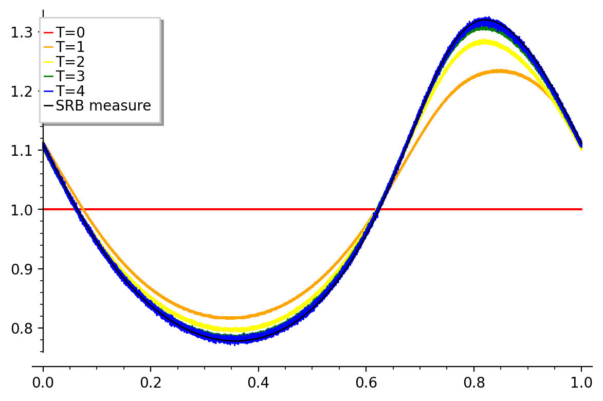

Let us explain the behaviour for small times. As a consequence of Theorem 2, for any , one has:
This is illustrated by Figure 5. See also [Gui15a, Theorem 12.17] for a proof with effective bounds on convergence speed. Roughly speaking, the operators , acting on invariant measures, converge towards . Hence, the behaviour of
is the “combination” of the behaviours of
| (1) | ||||
The second one is well understood, as tends to 0 exponentially fast in (combine Lemma 1 with the fact that the densities converge exponentially to the density of in the topology), so we are reduced to study the first map (1).


Figure 6 shows simulations of the first map (1). On these graphics there are three distinct time regimes:
- ()
The short-term behaviour, where the curves for discretizations seem to have a uniform behaviour: for a fixed time and the grid parameter going to infinity, they seem to converge to a curve that depends more or less exponentially on (it is close to a line on the right graph which is in logarithmic scale). For this regime we have a theoretical prediction given by the asymptotics (5) of Theorem 2. We will confront this prediction with the actual simulations in the sequel.
- ()
The medium term behaviour, where the curve globally grows slowly.
- ()
The long-term or asymptotic behaviour, where the curve is periodic (at least for small values of ).
These three different regimes will guide our study of (1). More precisely, we will study these three regime separately and one after the other.
As proved independently in [DV98] and [Flo02], for a generic map of , the roundoff errors equidistribute: for a fixed time , and the order going to infinity, the sequence of roundoff errors in time equidistributes in . See also [GM22, Proposition 3.2] for a more precise statement, which is obtained as a byproduct of the proofs.
So at first sight, one could expect the discretizations to behave very similarly to random perturbations. More precisely, the discretization ’s global dynamics may be thought as the typical global dynamics of the random map , acting on -tuples of points of such that each point of this tuple is randomly drawn uniformly in .
In fact, things are a bit more subtle, and one quickly realizes that the fact that orbits of can merge (i.e. that there exists distinct grid points that are eventually mapped to the same point under ) — and hence will stay together forever — must be an important parameter influencing the evolution of . With this in mind, one can isolate (at least) four phenomena that make the action of discretizations different from that of a random map.
- ()
The iterates of points always belong to .
- ()
Two points of having the same image by will have identical positive orbits.
- ()
The local shape around of the image is very similar to the one of a linearization of around the points , which is a model set (see [GM22]).
- ()
Any point eventually falls in a periodic cycle.
Part of the paper will be devoted to the understanding of the relative effects of these phenomena on the action of discretizations on measures.
Some bibliographical remarks
There are numerous numerical studies of the spatial discretization effects, but strangely only few works about these effects on ergodic properties.
A lot of these works focus on specific families of low-dimensional dynamics: [Bla98] for rotations and twist maps, [SB86] and [KMP99] for the tent map of slope , [Boy86] for a piecewise expanding map of slope , [DKP94] for (but for a random roundoff error model), [DKKP97, DKKP96, KMP99] for , [Cor92, CFM90] for the Gauss map… These articles mainly focus on combinatorial properties of discretizations: such discretizations are finite maps, hence their combinatorial properties are roughly determined by the family of lenghts of periodic orbits and the size of their basins of attraction. This focus on combinatorial properties seems to have been initiated in [Lev82].
In [Lan98], after some illuminating general remarks, Lanford carries numerical simulations of the expanding map . Although mainly combinatorial, one of them computes the measure carried by the longest detected cycle. On these simulations, these measures seem close to the SRB measure (the discretization is taken in the sense of the double precision).
More recently, Galatolo, Nisoli and Rojas [GNR14, Sections 6, 7 and 8] conducted numerical experiments on circle piecewise expanding maps (one example of which with a point with derivative 1) from an ergodic viewpoint. The difference with our study is that they consider Birkhoff averages of Dirac measures instead of the Lebesgue measure; their study is less extensive than ours but they still observe interesting behaviours of artefacts generated by roundoff errors. Their conclusion is that “These experiments show that, in general, using floating point arithmetics to compute Birkhoff averages and invariant measures should not be considered reliable, not because of truncation and rounding errors, but rather because the dynamics of the discretised map does not mirror the generic dynamic of the real map.”
There are few theoretical nontrivial results about the relations between discretizations and ergodic properties. In [GB88], Góra and Boyarsky get some theoretical results of convergence of the discretizations’ asymptotic measures (see (12)) towards , under the hypothesis that there exists large orbits for the discretization (of size for a fixed and any large enough). They check that this hypothesis holds for some piecewise linear maps of slope that are power of . However, [Gui19, Theorem 33] (see Theorem 3) shows that this hypothesis is not satisfied for generic dynamics…
In his PhD thesis [Flo02], Flockermann carries numerical simulations of maps which are similar to those considered in the present paper. However, these are mainly combinatorial: as in [Lan98], the only ergodic properties considered deal with the measure carried by some periodic orbits of the discretization. In this thesis the author also proves theoretical results about distribution of roundoff errors for generic circle expanding maps.
These results were obtained independently by Vladimirov in [Vla96] (further works based on this grounding article were published in [DV98, VKD00, DV02a, DV02b]). In this article, the author founds a solid theoretical basis about the discretizations’ behaviour, which revals more powerful than Flockermann’s approach: in addition to the equidistribution of roundoff errors, Vladimirov gets Theorem 3, and some functional central limit theorem, which was published with Vivaldi in [VV03]. Early apparitions of this kind of ideas can be found in the work of Voevodin [Voe67].
2. Preliminaries
2.1. Distance on measures
We will denote by the set of maps that are and expanding (meaning that for any .
In the first paper of this series [GM22], we give an asymptotics of the distance between the measures and , for fixed and going to infinity. This distance is measured by what we call the Cramér distance: if and are two probability measures on , and and are their respective repartition functions defined from the starting point 0, we set and
| (2) |
This is a distance spanning the weak-* topology on measures. For more details, see [GM22]. The following lemma is straightforward.
Lemma 1.
If and are two absolutely continuous probability measures on with respective densities with respect to Lebesgue measure and , then
Proof.
In this case we have, for any ,
and the same for , so
and
∎
We will also use the Ruelle-Perron-Frobenius (RPF) operator, defined on observables by
| (3) |
Note that if is the density of an absolutely continuous measure , then is the density of .
2.2. The maps used in the simulations
In our numerical studies, we will consider the following maps:
| (4) | ||||
with three parameters, with chosen such that the map is expanding (which is true if ).
In most of the simulations, we will take , and (and in this case the minimum of is bigger than ). See Figure 2 for a graph of this map.
For some simulations, we will consider small perturbations of this system, by choosing and , for
2.3. The code for the experiments
The code we used for experiment is based on the Python project CompInvMeas-Python [MNP15] developed as an initiative to unify the approach to the computation of invariant measures explained in [GN14] using SageMath [The22], the framework and related further developments will be fully described in the article in preparation [GMNP22]. The code used from the project was forked from an older version and contains facilities to work with dynamical systems, to compute the Perron-Frobenius operator of an expanding dynamical system and to retrieve the corresponding numeric fixed point.
When the dynamics is expanding with a factor it is possible to certify the error in the approximation of the SRB measure, estimating independently the numerical error which occurred while computing the numeric fixed point, and the mathematical error occurring representing the transfer operator with a finite-dimensional linear operator. While relevant, this estimation is very pessimistic therefore we used the result of the SRB measure in our experiments without adding the error coming from the rigorous error estimation, as it would have hidden the error coming from the spatial discretization.
Our experiments have been conducted in a notebook using the above facilities as a Python library, plus additionally a few support Python files offering facilities of our experiments. Such facilities are to compute different spatial discretizations of a dynamical system, to compute measure distances (Cramér and Wasserstein distance), and convenience functions to save intermediate results to a database in order to be able to interrupt experiments and resume them later. An end-to-end run of all the experiments takes several days and will create temporary files of roughly 500Gb.
The notebook with all the support file and the instructions to repeat the experiments is available on the url: https://github.com/maurimo/DiscretizedDynSys
3. Short term behaviour
3.1. Theoretical result for Cramér distance
Theorem 2 ([GM22]).
Let , a generic expanding map of the circle , and . Then
| (5) |
where stands for the scalar product, is the RPF transfer operator defined by (3), is the derivative and is the -th iterate of .

The aim of this section is to explore numerically the validity in practice of such results: the speed of convergence cannot be specified in the proof of Theorem 2 (it is hidden in the “generic” term).
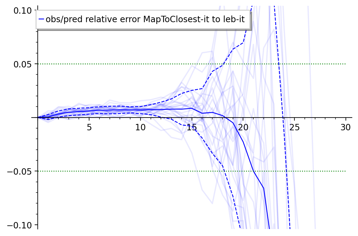

As can be seen on Figure 7, the theoretical prediction is quite good up to time 20 for . More precisely, as can be seen on the left of Figure 8, the theoretical prediction stops being relevant from time . Note that for , one has ; this behaviour of the time until when the theoretical prediction is accurate typically logarithmic in is strongly suggested by Figure 8, right. In can be explained heuristically in the following way: for , as the derivative of the map is everywhere close to 2, 20 is more or less the time needed for the iterations of a grid domain to become macroscopically visible.
Moral.
In practice, Theorem 2 is valid until times logarithmic in .
3.2. Rate of injectivity
Another quantity for which we have theoretical results is the rate of injectivity. It is defined as
This quantity (and the one studied in the next subsection) will be used in the study of the medium term behaviour of discretizations. In this subsection and the next one, we will:
- •
state theoretical results for these quantities, which will be proved for generic maps and small number of iterations;
- •
observe experimentally whether these theoretical results stay true in the short or medium term.
Before recalling the result of [Gui19], let us introduce some notations. Given an expanding map of of degree , the set of time- preimages of a point has a structure of complete -ary tree, whose vertices are the points for , and the edges are of the form . One labels each edge of this tree by the number , and denote by the resulting labelled graph (see Figure 9).
We call random graph associated to at the random subgraph of , such that the laws of appearance of the edges in are independent Bernoulli laws of parameter . In other words, is obtained from by erasing independently each vertex of with probability .
We define the mean density as the probability that in , there is at least one path linking the root to a leaf.
Theorem 3.
Let , a generic element of and . Then,
| (6) |
As a byproduct of the proof of this theorem (and in particular Lemma 34 of [Gui19]), we get the following local convergence result (see also [Vla96]).
Proposition 4.
For any , for a generic expanding map and for almost every point , one has
Note that a first step towards the proof of this theorem was realized in the unpublished thesis [Flo02].
The idea behind this theorem is the following. Assume for simplicity that , take some point , and denote its preimages by by and . Then, in the neighbourhood of , the set looks like the discretization22 2 Here, “discretization” stands for the projection on the nearest element of , i.e. the image under the projection on the nearest integer. of the set . But, still in the neighbourhood of , the “probability” for a point to be in the discretization of the set is equal to . One of the steps in the proof of Theorem 3 is to show that the probabilities coming from the different branches are independent: the probabilities for a point to be in the discretizations of the sets are independent.
The following lemma gives a practical way to compute the percolation probability , in terms of the transfer operator associated to (for which we have a fast and reliable algorithm).
Lemma 5.
For any ,
In particular, if the degree of satisfies , denoting , one has
It is possible to get similar formulae for bigger by using Vieta’s formulas.
Proof.
The first formula comes directly from the definition. The second one is a simple computation. ∎


Figure 10 compares the theoretical rate of injectivity (the one given by Theorem 3 and computed with the help of Lemma 5) with the actual rate of injectivity of a discretization , depending on the time .
Moral.
The predictions of Theorem 3 are really good during a quite long time (less than 5% up to time 200).
3.3. Local distribution of preimages
We pursue the study of the rate of injectivity by focusing on more precise quantities. We will look at the distribution of the number of preimages of a point of the grid. To do that, we set (which depends on the point and the time ) the probability that in , there are exactly paths linking the root with the leaves. Denote by
| (7) |
the associated generating series.
Of course, the polynomial is of degree at most and satisfies and .
The proof of Theorem 3 links the limiting behaviour, for , of the number of preimages of points of the grid , with the random behaviour of the tree . Hence, as a byproduct of this proof, one gets the following result (see also [Vla96]).
Proposition 6.
For any , for a generic expanding map and for almost every point , one has


In this case, the generating series formalism gives the following nice formula, that allows to compute the distributions by an iterating process involving the RPF operator .
Proposition 7.
If , then, denoting ,
Hence, denoting ,

Proof.
Direct computation of the probabilities. ∎
This proposition gives a fast algorithm to compute the distributions , as it allows to get it from iterations of for which we have a fast algorithm.
Figure 11 gathers both theoretical and real values of the local densities of preimages. For the actual values, we represent the quantities, for different integers , for a fixed discretization size and a fixed time ,
| (8) |
As can be seen on this figure, the predictions of Proposition 6 are quite accurate: the theoretical and actual curves match very well, up to time , for . In fact, these predictions stay accurate during quite a long time, as can be observed on Figure 12: for or , there is no big difference between the observed values and the prediction up to time 200. In fact, it seems that the theoretical predictions of Figures 10 and 12 stay accurate until a time comparable to .
Moral.
This suggests that the discretizations begin to deviate from these theoretical predictions when there is a significant proportion of points of that have fallen in a periodic orbit of .
4. Medium term behaviour
In [Lan98], Oscar E. Lanford proposes to study the dynamics of the maps in the regime . Note that in the view of the discussion of Section 5, one might be tempted to replace the last condition by , as sugested by Lanford himself (see also Figure 16 and the associated discussion). For the first condition , it is also justified by the previous study of the short term behaviour, as well as [Gui15a, Theorem 12.17].
For now, theoretical breakthroughs in Landford’s regime seem out of reach, which motivates a numerical study of discretizations in this case.
Recall the different phenomena isolated in the introduction, that can explain why the action of discretizations on measures differ from the one of the initial map .
- ()
The iterates of points always belong to .
- ()
Two points of having the same image by will have identical positive orbits.
- ()
The local shape around of the image is very similar to the one of a linearization of around the points , which is a model set (see [GM22]).
- ()
Any point eventually falls in a periodic cycle.
4.1. Different discretization schemes
To understand what influences the evolution of the distance between iterates of Lebesgue measure and iterates of the uniform measure under discretizations, we look at what happens when we change the definition of the discretized map. We will need the following notation: for , the integer is chosen such that ; it allows to set such that .
- •
MapToClosest: This is the already defined discretization of the map, where is defined as the point of closest to .
- •
OnceDecidedRandom: is a random map, such that for each , the point is chosen once for all and randomly (and independently) to be with probability , and to be with probability . Note that the iterations of two points under are independent iff .
- •
StepwiseRandom: is a random map quite similar to (OnceDecidedRandom), such that for each and at each iteration, the point is chosen randomly (and independently) to be with probability , and to be with probability .
- •
PointsRandomOnGrid: acts independently on -tuples of elements of as (StepwiseRandom):
Of course, this gives the measure
- •
PointsPerturbed: acts on -tuples of elements of as a random perturbation of : let be the random map obtained from by post-composing with a uniform noise on the segment (i.e. is chosen randomly and uniformly in ). Then
- •
MapToCombination: acts only on the measures on . It is affine, in the sense that for any convex combination , one has . And is defined by
Let us discuss the fundamental differences between these maps.
MapToClosest and OnceDecidedRandom have a quite similar definition, except that the first one is deterministic and the second one random. More precisely, there is the following difference between these maps: as is almost linear at a small scale, the image of under will depend deterministically on , while the image of under will depend only probabilistically on . In other words, for large enough, is locally almost (i.e. up to a set of arbitrarily small local density) a model set (for a definition and a study of this property, see [GM22] or [Gui19]), a property that does not possess. This will allow us to determine if the phenomenon ( P 3 ) has a detectable effect on the evolution of the distance (1) between and .
The difference between OnceDecidedRandom and StepwiseRandom is that the second one is not autonomous. Hence, almost surely, orbits for this map will not be pre-periodic, while all orbits of MapToClosest and OnceDecidedRandom are. This will allow us to determine if the phenomenon ( P 4 ) has an effect on the evolution of the distance (1).
An important feature of the three previous maps (MapToClosest, OnceDecidedRandom and StepwiseRandom) is that orbits that merge then stay together forever. The map PointsRandomOnGrid, which besides is quite similar to StepwiseRandom, does not have this property. A priori, does not imply that a.s. This will allow us to determine if ( P 2 ) affects the evolution of the distance (1).
All the four previous maps are based on the discretization grid . This is not the case for PointsPerturbed, which acts on -tuples of points of the circle. It can be seen as a continuous counterpart of PointsRandomOnGrid. This will allow us to determine if the phenomenon ( P 1 ) affects the evolution of (1).
Finally, MapToCombination is the only discretization type which splits measures 33 3 By Perron-Frobenius theorem, the measures obtained from MapToCombination tend (when the time goes to infinity) to some measure depending on . We do not know if these measures tend to when goes to infinity. It may be possible to prove it using the ideas of [GN14], by checking that the distance between both Perron-Frobenius and discretized (associated to MapToCombination) transfer operators are close relative to distance. As this is not in the scope of this article, we do not investigate this question..
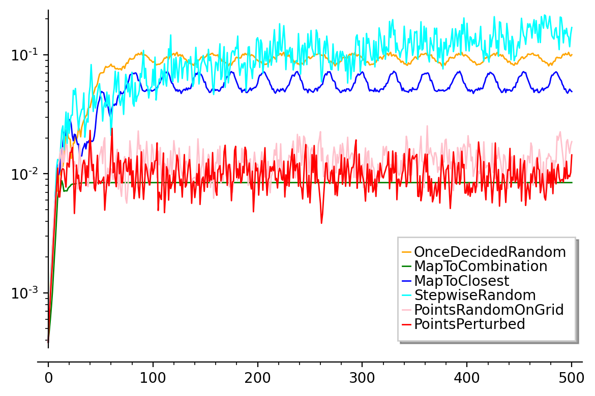
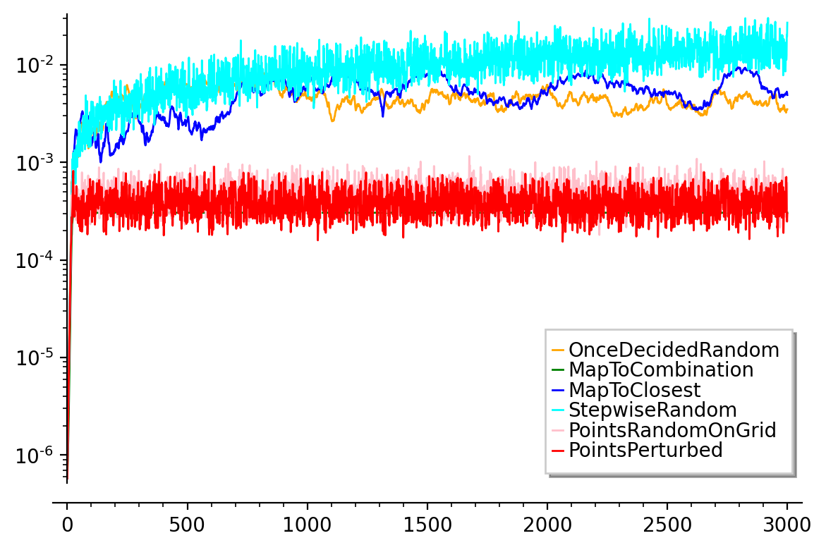
Figure 13 shows the evolution of the distance between the measures and the images of under the iterates of the different discretization types of : , , , , and .
On the left of this figure, where , there is no intermediate regime for the discretizations and : from time , the distance evolution becomes periodic. This can be explained by the fact that from this time, most of the grid’s points have fallen in a few cycles of the discretization: one directly jumps from the small term behaviour, which is described quite well by Theorem 2, to the periodic asymptotic regime. Indeed, in this case the limit time of short-term behaviour should be around , while the theoretical average time for orbits to cycle is (see Section 5).
For (Figure 13, right), this periodic asymptotic behaviour does not appear clearly for time : there is an actual medium term behaviour of discretizations.
Before studying further this intermediate regime, we first examine random point processes in the point of view of the distance with the initial measure.
4.2. Cramér distance between a measure and the random point process associated to it
We have seen that on the simulations we made, the theoretical estimates on the local distributions of preimages (Paragraphs 3.2 and 3.3) stay relevant in the middle term. Hence, they can be used to set a conjectural behaviour of the distance in the middle term. Let us first introduce some definitions.
Let be probability measures on , with the density of being given by the map (recall that was defined in (7) and described in Proposition 6). Let , , and set . Let also be the random probability measure defined by
where each point is chosen independently in , according to the measure . Suppose that for any ,
(meaning that we have this asymptotics when goes to infinity).
Conjecture 8.
In the regime and , the distance(1) is close to the expected value of the Cramér distance between the SRB measure and .
As a first step, before getting to the numerical study, we compute the expected value of the square of distance between the SRB measure and .
Let be a probability measure on . We identify with , and define as44 4 There is a conflict of notations with the dynamics , we hope that which one is used is clear from the context. the cumulative distribution function of minus its average (so that ). Let also be the primitive function of such that:
Remark that , and that . Finally, given , one defines to be the cumulative-minus-average distribution function of
The following theorem gives the expectation of the (square of the) distance between a measure and a point process associated to it.
Theorem 9.
Let and be probability measures on with respective repartition functions and .
Let , and set . Let also be the random probability measure defined by
where the points are chosen independently in , each one with distribution . Then
| (9) |
The proof of this theorem can be found in appendix.
The setting of this theorem will be applied in the case where can be written as (hence the are not probability measures), and the measures are the normalizations of the , with the being chosen such that the normalization factors are close to (see Remark 10).
Some similar estimations were obtained for the Wasserstein distance in [BL19], but the authors only manage to get bounds ant not exact values for the expected value.
Remark 10.
Note that being fixed, one can choose the family such that the first term is of order , while the second one is typically of order .
Indeed, suppose that the cumulative distribution function of satisfies , and for , let such that
Note that
so
and
Hence,
which gives a distance of the order of by Lemma 1.
On the other hand,
for any large enough. Hence, in this case, the dominating term in (9) is the second one.
The equality between the two lines of the theorem’s equation (9) comes from the following elementary lemma.
Lemma 11.
Let be a probability measure on , with distribution function minus average . Let be a primitive of such that . Then
A proof of this lemma can be found in appendix.
By taking for any , one gets the following corollary about point precesses with points of uniform weights.
Corollary 12.
Let be a probability measure on , , and be the random measure defined by
where the ’s are iid points with distribution . Then
| (10) |
Remark 13.
A simple computation shows that the square of the distance between equispaced points and Lebesgue measure, is equal to . On the other hand, one has .
Hence, the expectation of the square of the Cramér distance of the uniform point process (with all weights equal to 1) is . In this case, the squared distance for a typical point process is way bigger than the minimal squared distance for the same number of points (it is of the order of its square).
4.3. Comparison between the random point process and the discretization


Now we have defined different discretization types in Paragraph 4.1 and got a theoretical estimate of the distance between a measure and the random point process associated to it paragraph 4.2, we can compare them numerically.
Figure 14 displays the mean values as well as the mean values standard deviation of the Cramér distance between the iterates of the discrete measure by the discretization type and the iterate of Lebesgue measure by RPF operator, for all the discretization types defined in Paragraph 4.1.
It also shows the the theoretical prediction for small times given by Theorem 2, and the curves of two expected values of the distance between SRB measure and a point process. The first one, in violet, is obtained from Corollary 12 ; it is square root of the expected value of the square of the distance between the SRB measure and the measure made of independent random points with respect to this SRB measure. The second one, in pink, is cooked from Theorem 9 and the local distribution of preimages given by Proposition 6 in the following way: for each time , we compute the theoretical local distribution of preimages by the algorithm given by Proposition 7. To each of these functions , which represent local densities of measures (which we normalize to get probability measures), are associated a repartition functions . This allows to get an estimation by means of (9) (see also Remark 10)
| (11) |
At first glance, we can group the discretization types in three different clusters.
- (C1)
A first one containing only MapToCombination, whose asymptotic behaviour looks stationary, the asymptotic average distance is smaller than the estimation disc to m-random for SRB.
- (C2)
A second one containing PointsRandomOnGrid and PointsPerturbed. These two types of discretization give asymptotic behaviours similar to the estimation disc to m-random for SRB.
- (C3)
A third one containing MapToClosest, OnceDecidedRandom and StepwiseRandom. These three types of discretization behave asymptotically more or less as disc to m-random for lebit given by the map .
However, a closer look at each cluster reveals small differences.
For (C2), while the average value for PointsPerturbed follows asymptotically very well the curve of disc to m-random for SRB, the discretization type PointsRandomOnGrid has a significantly greater average asymptotic value. This is quite unexpected, as the difference induced by replacing the SRB measure by the projection of it on (by mean of ) in Corollary 12 is of order , and hence is negligible with respect to the orders of the computed distances, which are of order . We have no explanation to this phenomenon.
For (C3), the curves associated to MapToClosest and OnceDecidedRandom are very similar (see also Figure 15). Hence, the already discussed difference between microscopic behaviours of these discretizations, the first one having deterministic local correlations and the second one random local correlations, seems to have no impact on the asymptotics of the distance between measures. Moreover, the curves corresponding to StepwiseRandom, although also following quite well the curve of , behaves a bit more erratically than the two other ones (this is even more blatent on Figure 13).

Simulations over a larger time range show that the average distance for StepwiseRandom, form a certain point, gets bigger than the one for MapToClosest and OnceDecidedRandom. More precisely, Figure 15 shows this distance for times and . On this simulation, we can see that this time where the mean distances start to be different is more or less . This time is to be compared with the mean time necessary for an orbit to cycle for a typical map of elements, which is : from this time 137, a significant part of orbits have cycled, which perturbs the process of injectivity loss. Note that on Figure 15 we have not represented the prediction that we discussed in the beginning of this paragraph, as in this time range accurate computations are out of our machine capacities: in the simulations we have to truncate the series up to some to avoid exponential explosion of data depending on simulation time; we checked empirically that this truncation does not affect the prediction by verifying that the predictions are the same weather we truncate up to or . The threshold we chose for the simulations () gives similar results to for times (as in Figure 14) but not (as in Figure 15); a larger threshold for time would make the computations extremely long and memory costing.
From these observations, one can conclude the following moral.
Moral.
The main phenomenon influencing the middle term behaviour of is the fact that orbits under merge. More precisely, the distance between and is rather well described by the distance between the SRB measure and the point process described by (see (11)): locally around , the proportion of points with weight of this process is equal to , where represents the local proportion of points around that have preimages under .
Note that in the simulations we performed the “middle term” is not that long and it may be that the phenomena specific to the short and long term still interfere in the time range and the discretization orders we chose: as noticed in Figure 13, left, for smaller orders there is even no middle term transitory behaviour. We would need more computing power to test the validity of the prediction (11) on bigger orders (typically close to ).
5. Long term behaviour
From Figure 3, one can wonder whether the quantity
which depends on , tends to 0 when the discretization parameter goes to infinity or not. According to the simulations (see Figure 17), it seems that yes, but unfortunately the proof of this result seems unreachable for now.
Let us first recall the fact that the maps are finite, so that every orbit eventually falls in a periodic cycle. Hence, one can characterize the expression ‘‘asymptotic regime’’ by the fact that all points have already browsed a whole periodic orbit55 5 In practical, we will see the asymptotic regime’s behaviour as soon as most of points of already have browsed a whole cycle.. Figure 16 shows the average of this time over points of depending on .

One can observe that this quantity behaves more or less as the same quantity for a typical random map on a set of elements, which is equivalent to (see [Bol01]); this equivalent is represented in black in Figure 16. This quantity is around for (which is the classical precision used by computers). Hence, in practical, one usually does not reach the asymptotic regime when iterating a map.
There is a canonical measure associated to the asymptotic regime in the following way. Fix , and let be the uniform measure on the grid . The measures converge in the Cesàro mean towards a measure
| (12) |
This measure is supported in the union of the periodic cycles of , the total weight of each of them being proportional to the size of its basin of attraction.
Question 14.
Do we have (in the weak-* topology) for a generic expanding map ?


Numerical experiments suggest that the answer to this question might be yes, as shown by Figure 17. Note that the convergence, if happens, is extremely slow: it would give a terrible algorithm to compute an approximation of the SRB measure.
However, it is possible that these simulations are misleading. As observed in [Gui15a] (see Figures 12.14 and 12.17), for some area-preserving diffeomorphisms of the torus, the measures seem to converge to the area for a set of of density 1, but there are still rare values of for which the distance between and the area stay at positive distance. Such a behaviour can be observed on Figure 18: while for most of the 100 discretization orders between and , the distance between the SRB measure and is around , for two of these discretization orders, the distance is bigger than (a distance that is no longer attained after on Figure 17).
Moral.
Our simulations do not suggest a clear conjecture about the convergence or not of towards , but it seems that this convergence holds for a subsequence of of density 1.

6. Conclusion
We have identidfied three different temporal regimes and, for each one, proposed a model to describe it.
The first one, ( R 1 ), studied in Section 3, is the short term. It occurs for times . In this regime, iterates of points that are initially microscopically close stay at a microscopical distance one from the others. The evolution of (1) is well described by Theorem 3.
The second one, ( R 2 ), is the middle term, studied in Section 4. It seems to occur for times and . In this regime, orbits of points that were neighbours at time 0 are typically at a macroscopic distance one from the other. Our simulations suggest that the main phenomena governing the evolution of (1) in this regime is ( P 2 ): two points of the grid having the same image by will have identical positive orbits. On our simulations, the behaviour of (1) looks a lot like the one of a random process described in Paragraph 4.2 (see (11)). This is a point process made of points with different weights, the local density of the points with weight being equal to the predicted local density of points with preimages under the discretization , this prediction being made by Proposition 6 (which reflects Phenomenon ( P 2 )). The expected Cramér distance between the point process and the SRB measure is given by Theorem 9.
The third one, ( R 3 ), the long term, is studied in Section 5. It should happen for (or maybe , or ). What is the right model for this regime is more unclear than for the two other ones. It seems like that, as observed in the litterature (e.g. [Flo02, Lan98, ERDF83, Mie05, DKKP96, Bin92, Lev82]), the combinatorial behaviour is well described by the one of a random map on a set with elements. Note that for some classes of interval maps having 0 as a fixed point, the combinatorial behaviour seem to be well described by a specific type of random mpas called random maps with a single attractive centre [DKPV95, DSKP96]. Even if our simulations suggest that the asymptotic measures may converge towards when goes to , this conclusion is not so clear in view of phenomena such as rare orders for which the measure is for away from SRB [Gui15b, Gui15a].
Of course, it is natural to ask whether such numerical phenomena hold in higher dimensions for systems with some hyperbolic properties (Anosov or Axiom A systems, systems with dominated splittings, etc.).
It is indeed a real challenge to tackle a theoretical validation of the numerical observations we outlined in this paper. As written by Lanford in [Lan98], “[…] this problem may be as hard of that of non-equilibrium statistical mechanics.”
We woulk like to put forward some research tracks that may be the first ones to address. First, one could try to get explicit times of convergence in Theorems 2 and 3 for some specific examples of piecewise real-analytic maps. Going a bit further, understanding why the first one is valid only in the short term and the second one remains true in the medium term would be an exceptionnal progress.
Also, adapting the proofs of [GM22] to the case of infinite branches circle expanding maps (e.g. Gauss map) may suggest other research directions. The program of previous paragraph may also be addressed in the case of the -shift (): the constant slope of the map may allow to undestand completely the discretizations’ behaviours.
Appendix A Proof of Theorem 9 and Lemma 11
Proof of Lemma 11.
One has
so
This proves the equality of the lemma.
We now prove the inequality. We first suppose that is a convex combination of maps , where is the cumulative-minus-average distribution function of . For we have the equality
If , with and , , then
Notice that fixing , we have
| (13) |
so for any we have . This proves that in the case is a convex combination of maps . The general case comes from the density (in norm) of such convex combinations among zero-average maps.
Note that a simple additional argument shows that we have equality iff for some . ∎
Proof of Theorem 9.
Given two probability measures and , the square of their Cramér distance is obtained as
where are the cumulative distribution function minus their average (as defined before Theorem 9). In our case we want to compute the expectation of the square of the Cramér distance between the measure and the random measure (which depends on the random points ). In this case, the (random) function is given by
where is the cumulative-minus-average distribution function of , and (note that they satisfy ). Each point will be chosen randomly and independently with distribution
First, suppose that the distribution functions of are differentiable; in this case is equal to the density of . Note that in this case , so that all further applications of Fubini’s theorem will be valid.
Keeping implicit that we will be averaging over chosen at random in with distribution , the square of the Cramér distance can be computed as
In each integral the average will only be over (or in the last one), as the integrand does not depend on , for . Each follows the distribution . Therefore we can simplify the sums of equal values and see the integrals as integral in just (or in the last integral). We can write:
| (14) |
Before deducing a general formula we well state two trivial lemmas.
Lemma 15.
For all we have:
In particular, we get .
Lemma 16.
In particular we get .
The expression (13) is valid on the half of the square where , therefore we have (applying the above lemmas and the fact that )
| (15) |
For of (14) we have
| (16) |
while for the second integral
| (17) |
Joining all simplified expressions (17), (16) and (15), we deduce that (14) can be rewritten as
which gives the first formula of the theorem. The second one is a consequence of Lemma 11
We now treat the general case for . The cadlag map can be approached in uniform topology by a smooth repartition function of a measure , which is close to in weak-* topology. It then suffices to remark that in (10), the left side is continuous in for weak-* topology, and right side is continuous in for the uniform topology. ∎
References
- [Bin92] Philippe M. Binder, Limit cycles in a quadratic discrete iteration, Phys. D 57 (1992), no. 1-2, 31–38.
- [BL19] Sergey Bobkov and Michel Ledoux, One-dimensional empirical measures, order statistics, and kantorovich transport distances, Memoirs of the American Mathematical Society 261 (2019), 0–0.
- [Bla98] Michael Blank, Discreteness and continuity in problems of chaotic dynamics, The American mathematical monthly 105 (1998), no. 3, 299– (eng).
- [Bol01] Béla Bollobás, Random graphs, seconde ed., Cambridge University Press, 2001.
- [Boy86] Abraham Boyarsky, Computer orbits, Comput. Math. Appl. Ser. A 12 (1986), no. 10, 1057–1064.
- [CFM90] Robert M. Corless, Gregory W. Frank, and J. Graham Monroe, Chaos and continued fractions, Phys. D 46 (1990), no. 2, 241–253. MR 1083721
- [Cor92] Robert M. Corless, Continued fractions and chaos, Amer. Math. Monthly 99 (1992), no. 3, 203–215. MR 1216205
- [DKKP96] Phil Diamond, Anthony Klemm, Peter Kloeden, and Alexei Pokrovskii, Basin of attraction of cycles of discretizations of dynamical systems with SRB invariant measures, J. Statist. Phys. 84 (1996), no. 3-4, 713–733. MR 1400185 (97i:58102)
- [DKKP97] Phil Diamond, Victor Kozyakin, Peter Kloeden, and Alexei Pokrovskii, A model for roundoff and collapse in computation of chaotic dynamical systems, Math. Comput. Simulation 44 (1997), no. 2, 163–185. MR 1481914 (99a:58114)
- [DKP94] Phil Diamond, Peter Kloeden, and Alexei V. Pokrovskii, An invariant measure arising in computer simulation of a chaotic dynamical system, J. Nonlinear Sci. 4 (1994), no. 1, 59–68. MR 1258483 (94m:58136)
- [DKPV95] Phil Diamond, Peter Kloeden, Alexei V. Pokrovskii, and Alexander Vladimirov, Collapsing effects in numerical simulation of a class of chaotic dynamical systems and random mappings with a single attracting centre, Phys. D 86 (1995), no. 4, 559–571. MR 1353178 (96e:58098)
- [DM07] Jérôme Dedecker and Florence Merlevède, The empirical distribution function for dependent variables: asymptotic and nonasymptotic results in , ESAIM, Probab. Stat. 11 (2007), 102–114.
- [DSKP96] Phil Diamond, M. Suzuki, Peter Kloeden, and Alexei Pokrovskii, Statistical properties of discretizations of a class of chaotic dynamical systems, Comput. Math. Appl. 31 (1996), no. 11, 83–95. MR 1392078 (96m:58164)
- [DV98] Phil Diamond and Igor Vladimirov, Asymptotic independence and uniform distribution of quantization errors for spatially discretized dynamical systems, Internat. J. Bifur. Chaos Appl. Sci. Engrg. 8 (1998), no. 7, 1479–1490.
- [DV02a] by same author, Branching processes and computational collapse of discretized unimodal mappings, Internat. J. Bifur. Chaos Appl. Sci. Engrg. 12 (2002), no. 12, 2847–2867.
- [DV02b] by same author, Set-valued Markov chains and negative semitrajectories of discretized dynamical systems, J. Nonlinear Sci. 12 (2002), no. 2, 113–141.
- [ERDF83] T. Erber, T. M. Rynne, W. F. Darsow, and M. J. Frank, The simulation of random processes on digital computers: unavoidable order, J. Comput. Phys. 49 (1983), no. 3, 394–419.
- [Flo02] Paul Philipp Flockermann, Discretizations of expanding maps, Ph.D. thesis, ETH (Zurich), 2002.
- [GB88] Paweł Góra and Abraham Boyarsky, Why computers like lebesgue measure, Comput. Math. Appl. 16 (1988), no. 4, 321–329.
- [GM22] Pierre-Antoine Guihéneuf and Maurizio Monge, Cramér distance and discretizations of circle expanding maps I: theory, 2022, arXiv 2206.07991.
- [GMNP22] Stefano Galatolo, Maurizio Monge, Isaia Nisoli, and Federico Poloni, A general framework for the rigorous computation of invariant densities and the coarse-fine strategy, 2022, in preparation.
- [GN14] Stefano Galatolo and Isaia Nisoli, An elementary approach to rigorous approximation of invariant measures, SIAM Journal on Applied Dynamical Systems 13 (2014), no. 2, 958–985.
- [GNR14] Stefano Galatolo, Isaia Nisoli, and Cristóbal Rojas, Probability, statistics and computation in dynamical systems, Math. Structures Comput. Sci. 24 (2014), no. 3, e240304, 25.
- [Gui15a] Pierre-Antoine Guihéneuf, Discrétisations spatiales de systèmes dynamiques génériques, Ph.D. thesis, Université Paris-Sud, 2015.
- [Gui15b] by same author, Dynamical properties of spatial discretizations of a generic homeomorphism, Ergodic Theory Dynam. Systems 35 (2015), no. 5, 1474–1523.
- [Gui15c] by same author, Physical measures of discretizations of generic diffeomorphisms, to appear in Ergodic Theory and Dynamical Systems, arXiv:1510.00720, 2015.
- [Gui19] by same author, Degree of recurrence of generic diffeomorphisms, Discrete Anal. (2019), Paper No. 1, 43.
- [KMP99] Peter Kloeden, Jamie Mustard, and Alexei V. Pokrovskii, Statistical properties of some spatially discretized dynamical systems, Z. Angew. Math. Phys. 50 (1999), no. 4, 638–660. MR 1709708 (2000e:37039)
- [Lan98] Oscar E. Lanford, Informal remarks on the orbit structure of discrete approximations to chaotic maps, Experiment. Math. 7 (1998), no. 4, 317–324.
- [Lev82] Yves-Emmanuel Levy, Some remarks about computer studies of dynamical systems, Phys. Lett. A 88 (1982), no. 1, 1–3.
- [Mie05] Tomasz Miernowski, Dynamique discrétisée et stochastique, géométrie conforme, Ph.D. thesis, ÉNS de Lyon, 2005.
- [MNP15] Maurizio Monge, Isaia Nisoli, and Federico Poloni, CompInvMeas-Python, Computation of Invariant Measures in Python, 2015, https://bitbucket.org/fph/compinvmeas-python/src/master/.
- [Rac91] Svetlozar T. Rachev, Probability metrics and the stability of stochastic models, Wiley Series in Probability and Mathematical Statistics: Applied Probability and Statistics, John Wiley & Sons, Ltd., Chichester, 1991.
- [SB86] Manuel Scarowsky and Abraham Boyarsky, Long periodic orbits of the triangle map, Proc. Amer. Math. Soc. 97 (1986), no. 2, 247–254.
- [The22] The Sage Developers, Sagemath, the Sage Mathematics Software System (Version 9.2), 2022, https://www.sagemath.org.
- [VKD00] Igor Vladimirov, Nikolai Kuznetsov, and Phil Diamond, Frequency measurability, algebras of quasiperiodic sets and spatial discretizations of smooth dynamical systems, Math. Comput. Simulation 52 (2000), no. 3-4, 251–272.
- [Vla96] Igor Vladimirov, Quantized linear systems on integer lattices: a frequency-based approach, CADSEM Reports, Geelong, Australia: Center for Applied Dynamical Systems and Environmental Modeling, Deakin University 96-032, 96-033 (1996), Parts I,II.
- [Voe67] Valentin V. Voevodin, The asymptotic distribution of round-off errors in linear transformations, Ž. Vyčisl. Mat i Mat. Fiz. 7 (1967), 965–976.
- [VV03] Franco Vivaldi and Igor Vladimirov, Pseudo-randomness of round-off errors in discretized linear maps on the plane, Internat. J. Bifur. Chaos Appl. Sci. Engrg. 13 (2003), no. 11, 3373–3393.