跳到论文正文
W Papers独立论文阅读器 arXiv:2206.07944 论文正文 计算阅读时间 · 0%
引用这篇论文根据当前论文元数据生成,正式投稿前建议核对。


License: CC BY 4.0
arXiv:2206.07944v4 [math.OC] 03 Aug 2023

Distributed Online Private Learning of Convex Nondecomposable Objectives

Huqiang Cheng    Xiaofeng Liao    and Huaqing Li    Thanks: H. Cheng and X. Liao are with Key Laboratory of Dependable Services Computing in Cyber Physical Society-Ministry of Education, College of Computer Science, Chongqing University, Chongqing, China, 400044.
E-mail: huqiangcheng@126.com; xfliao@cqu.edu.cn.(Corresponding author: Xiaofeng Liao.) H. Li is with Chongqing Key Laboratory of Nonlinear Circuits and Intelligent Information Processing, College of Electronic and Information Engineering, Southwest University, Chongqing, China, 400715.
E-mail: huaqingli@swu.edu.cn.
Abstract

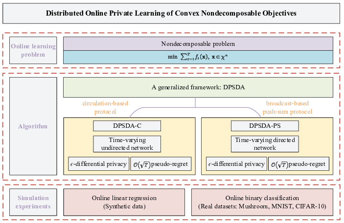
In the machine learning domain, datasets share several new features, including distributed storage, high velocity, and privacy concerns, which naturally requires the development of distributed privacy-preserving algorithms. Moreover, nodes (e.g., learners, sensors, GPUs, mobiles, etc.) in the real networks usually process tasks in real time, which inevitably requires nodes to have online learning capabilities. Therefore, we deal with a general distributed constrained online learning problem with privacy over time-varying networks, where a class of nondecomposable objectives are considered. Under this setting, each node only controls a part of the global decision, and the goal of all nodes is to collaboratively minimize the global cost over a time horizon TT while guarantees the security of the transmitted information. For such problems, we first design a novel generic algorithm framework, named as DPSDA, of differentially private distributed online learning using the Laplace mechanism and the stochastic variants of dual averaging method. Note that in the dual updates, all nodes of DPSDA employ the noise-corrupted gradients for more generality. Then, we propose two algorithms, named as DPSDA-C and DPSDA-PS, under this framework. In DPSDA-C, the nodes implement a circulation-based communication in the primal updates so as to alleviate the disagreements over time-varying undirected networks. In addition, for the extension to time-varying directed ones, the nodes implement the broadcast-based push-sum dynamics in DPSDA-PS, which can achieve average consensus over arbitrary directed networks. Theoretical results show that both algorithms attain an expected regret upper bound in 𝒪⁡(T)\mathcal{O}(\sqrt{T}) when the objective function is convex, which matches the best utility achievable by cutting-edge algorithms. Finally, numerous numerical experiments on both synthetic and real-world datasets verify the effectiveness of our algorithms.

Index Terms: 
Differential privacy, nondecomposable problem, distributed online learning, time-varying networks.

I Introduction

More recently, there has been an increasing interest in distributed learning problems arising from its extensive use in areas like machine learning [1], sensor network [2], smart grids [3], and so on. A distinctive feature of this class of problems is that all nodes collaboratively solve a learning problem without knowledge of the global gradient information. In the setting, nodes transmit local estimates to each other with its immediate neighbors, which in turn makes nodes converge asymptotically to the optimal point. Based on the system in which the learning occurs, the methods are categorized into two types, namely, offline and online algorithms.The former solves a fixed problem, while the latter works on a time-varying and uncertain one.

I-A Related Works

Distributed offline learning: The study of distributed offline algorithm is relatively mature, such as subgradient-push [4], primal-dual [5, 6], gradient tracking [7, 8, 9], stochastic optimization [10], asynchronous optimization [11, 12], etc. Generally, the algorithm is said to be elegant if it achieves a linear rate 𝒪⁡(at)\mathcal{O}\left(a^{t}\right), 0<a<10<a<1, for strongly convex objectives or a sublinear rate 𝒪⁡(1/t2)\mathcal{O}(1/t^{2}) for convex ones, where tt denotes the update counter.

Distributed online learning: In practice, a host of application scenarios are dynamic, and data often needs online processing to respond quickly to the real-time needs of users. For example, many people are always keen on online activities, such as watching videos, reading news, shopping, and so on. In order to increase advertising revenue, IT companies have to provide quality ad push services for each user based on their browsing data. As users’ online activities are dynamic and uncertain over time, the task of sampling data on all users needs to be performed repeatedly. In consequence, handling nearly petabytes of data every day is their daily routine. Thus, this naturally calls for online learning capabilities. In recent years, various types of distributed online algorithms have been developed, such as ADMM-based [13, 14], primal-dual [15, 16, 17], dual-averaging [18, 19], weight-balancing [20], subgradient-push [21], mirror descent [22, 23] and so on.

To measure the real-time performance, [24] presented a standard metric called as regret. Note that an online learning algorithm is claimed to be good if its regret is sublinear. It is well known that the optimal regret bound is an order 𝒪⁡(T)\mathcal{O}(\sqrt{T}) (resp. 𝒪⁡(log⁡T)\mathcal{O}(\log T)) for convex (resp. strongly convex) objectives.

Nevertheless, high volumes of online learning data may involve in some serious personal information, e.g., salary or medical records. Due to the distributed network topology, the information is transmitted and processed through mutual communication between neighboring nodes. The information may be eavesdropped during the transmission, which may lead to the leakage of sensitive information. To address the privacy concern, this paper mainly focuses on the differential privacy mechanism [25], which scrambles the sharing information by adding a certain amount of noise, thus making it impossible for an attacker to learn the users’ private data. Differential privacy has developed extremely rich mathematical formulation and provable privacy properties. A basic way to enable differential privacy involves injecting the noise or bias in the nodes’ communication or computation.

Differential privacy: Some works on differential privacy algorithms have been available. Zhu et al. [27] developed a private online algorithm using a weight-balancing technique. Employing the Laplacian mechanism, a differential privacy version of the online subgradient-push algorithm [21] was presented in [28] for time-varying directed networks. In [27, 28], only the unconstrained optimization problems are considered. For the constrained problems, Xiong et al. [29] proposed a subgradient rescaling privacy-preserving algorithm over fixed directed networks. Moreover, Han et al. in [30] and [31] considered two privacy versions of the work [18] by using uncorrelated and correlated perturbation mechanisms, respectively. In [32], a differential privacy by functional perturbation is achieved, but it is limited due to the requirement of squared integrability on the objective functions.

All of the above literature on differential privacy requires a decomposable system objective function ft​(𝐱)f_{t}\left(\mathbf{x}\right), i.e., ft​(𝐱)=∑i=1nfi,t​(𝐱)f_{t}\left(\mathbf{x}\right)=\sum\nolimits_{i=1}^{n}{f_{i,t}\left(\mathbf{x}\right)}, in which any local objective fi,tf_{i,t} is just revealed to node ii at time tt. In this case, each node ii holds and updates an estimate 𝐱i∈ℝd\mathbf{x}_{i}\in\mathbb{R}^{d} that converges asymptotically to the best decision 𝐱∗∈ℝd\mathbf{x}^{\ast}\in\mathbb{R}^{d} of the system problem. Note that the dimension dd is possibly consistent with the number of nodes nn or not. However, some system functions ft​(𝐱)f_{t}\left(\mathbf{x}\right) may not allow natural decompositions, and the decision variable 𝐱=[(𝐱1)⊤,⋯,(𝐱n)⊤]⊤∈ℝd\mathbf{x}=[(\mathbf{x}_{1})^{\top},\cdots,(\mathbf{x}_{n})^{\top}]^{\top}\in\mathbb{R}^{d} is distributed among the nodes. In this scenario, every node ii only controls a part 𝐱i∈ℝdi\mathbf{x}_{i}\in\mathbb{R}^{d_{i}} with ∑i=1ndi=d\sum\nolimits_{i=1}^{n}{d_{i}}=d, that converges asymptotically to the ii-th part of 𝐱∗\mathbf{x}^{\ast}. Fig. 1 further portrays the estimated behaviors of the decision variable 𝐱\mathbf{x} in the two problems. Each node only controls a coordinate of the decision variable in the nondecomposable problems (see Fig. 1(a)), while each node maintains a full estimate of the decision variable in decomposable setting (see Fig. 1(b)).

Refer to caption
Fig. 1: The behaviors of the decision variable in nondecomposable problems (a) and decomposable problems (b).

Motivations: Distributed methods for solving nondecomposable problems have been considered in [19, 33, 34, 35, 36, 37, 38]. References [33, 34, 35, 36, 38] are oriented towards distributed offline problems. In [37], an online local dynamic programming algorithm is presented, while Lee et al. [19] developed two online coordinate dual averaging algorithms. Regrettably, the privacy concerns are ignored in the existing works. Compared to the well-studied differential privacy on decomposable problems, how to do differential privacy on nondecomposable ones remains largely unexplored. It is of interest, therefore, to apply privacy mechanisms to the nondecomposable problems.

TABLE I: Related References
Reference Digraph Constraint Nondecomposability Private
[21] ✓ ×\times ×\times ×\times
[18] ×\times ✓ ×\times ×\times
[19] ✓ ✓ ✓ ×\times
[27, 28] ✓ ×\times ×\times ✓
[29, 30] ✓ ✓ ×\times ✓
[45] ×\times ✓ ×\times ✓
Our work ✓ ✓ ✓ ✓

I-B Contributions

In this study, we are committed to a structured investigation of differentially private distributed online for nondecomposable problems. A comparison of our work with the cutting-edge works is reported in TABLE 1. To begin with, we formulate a differentially private stochastic dual-averaging distributed online framework, named as DPSDA. Specifically, we inject the Laplace noise to perturb the dual variables so that the execution of the algorithm has the approximate output on a pair of adjacent datasets (cf. Definition 1), which in turn makes it infeasible for the attacker to infer the true data. Then the Nesterov’s dual-averaging subgradient method [40] is adopted in DPSDA as a learning subroutine. For all that we know, DPSDA is the first formal framework of differentially private distributed online learning protocol for nondecomposable problems.

In line with the rules of DPSDA, we design two differentially private distributed online learning algorithms. One employs the circulation-based protocol [39] for undirected communication (named as DPSDA-C), while the other utilizes the push-sum method [4] for the directed communication (named as DPSDA-PS). To be more general, the dual averaging steps of both algorithms use the noise-corrupted gradients instead of the exact gradients. This arises from numerous applications as well, including distributed learning over the network and recursive regression. It is important, but not trivial, to extend this since the stochastic gradient error of each node is spread to other nodes in real time through the communication, making the dynamics statistically dependent on time and nodes.

We further conduct a rigorous expected regret analysis on DPSDA-C and DPSDA-PS. The results show that both algorithms attain an expected regret 𝒪⁡(T)\mathcal{O}(\sqrt{T}) for convex objective functions, which matches the best utility achievable by cutting-edge algorithms. Moreover, the derived expected regret bounds capture explicitly the effect of privacy level, vector dimension, network size, and network topology. Besides, our results concerning differential privacy reveal an inevitable trade-off between privacy levels and algorithms accuracy.

I-C Organization and Notations

The latter sections of this study are scheduled as follows. Section 2 introduces several fundamentals about the problem of interest. In Section 3, we present DPSDA and a basic regret bound. DPSDA-C and its analysis are given in Section 4, while DPSDA-PS and its analysis are presented in Section 5. Then, Section 6 conducts numerical experiments to confirm the theoretical findings. Finally, Section 7 briefly provides some remarks on this study.

The notations of this paper are listed below.

Notation Definition
zz, 𝐳\mathbf{z}, and ZZ scalar, column vector, and matrix
ℝd\mathbb{R}^{d}, ℝ\mathbb{R}, ℤ0\mathbb{Z}_{0}, and ℤ+\mathbb{Z}_{+} the set of dd-dimensional real vector, real numbers, nonnegative integers, and positive integers
𝟏d\mathbf{1}_{d} and InI_{n} the dd-dimensional all-one vector and the n×nn\times n identity matrix
[A]i​j\left[A\right]_{ij} and (A)⊤(A)^{\top} the (i,j)(i,j)-th entry and the transpose of matrix AA
⟨⋅,⋅⟩\left<\cdot,\cdot\right> the inner product
∥⋅∥\lVert\cdot\rVert and ∥⋅∥1\lVert\cdot\rVert_{1} the 22-norm and the 11-norm
𝐞i\mathbf{e}_{i} the vector with the ii-th entry being 11 and the others being 00
δik\delta_{i}^{k} the Kronecker delta symbol, i.e., δik=1\delta_{i}^{k}=1 if i=ki=k and δik=0\delta_{i}^{k}=0 otherwise
Lap​(σ)\text{Lap}\left(\sigma\right) with σ>0\sigma>0 the Laplace distribution with probability density function pσ​(𝐱)=12​σ​exp⁡(−|𝐱|σ)p_{\sigma}\left(\mathbf{x}\right)=\frac{1}{2\sigma}\exp(-\frac{\left|\mathbf{x}\right|}{\sigma})
𝔼⁡(⋅)\mathbb{E}\left(\cdot\right) and ℙ⁡(⋅)\mathbb{P}\left(\cdot\right) the expectation and probability distribution
A⁡(t:s)A\left(t:s\right) with t≥s≥0t\geq s\geq 0 the product of the time-varying matrix sequence {A⁡(k)}k=st\left\{A\left(k\right)\right\}_{k=s}^{t}, i.e., A(t)⋯A(s)A\left(t\right)\cdots A\left(s\right). In particular, A⁡(t−1:t)≜InA\left(t-1:t\right)\triangleq I_{n} with t≥1t\!\geq\!1.

II Preliminaries

We provide several preliminary materials, including graph theory, problems of interest, as well as differential privacy.

II-A Graph Theory

Consider a general network with nn nodes, indicated by elements of the set 𝒱={1,⋯,n}\mathcal{V}=\left\{1,\cdots,n\right\}. The network topology specifies the local communication between nodes, which is usually modeled by one of the following two graphs:

  1. i)

    One is the time-varying undirected graphs 𝒢1​(t)=(𝒱,ℰ⁡(t))\mathcal{G}_{1}\left(t\right)=\left(\mathcal{V},\mathcal{E}\left(t\right)\right). Here, ℰ⁡(t)\mathcal{E}\left(t\right) is an undirected edge set at time tt. That is, if (i,j)∈ℰ⁡(t)\left(i,j\right)\in\mathcal{E}\left(t\right), then nodes ii and jj can send messages to each other at time tt. Let 𝒩i(t)={j∈𝒱|(i,j)∈ℰ(t)}∪{i}\mathcal{N}_{i}\left(t\right)=\left\{j\in\mathcal{V}\left|\left(i,j\right)\in\mathcal{E}\left(t\right)\right.\right\}\cup\left\{i\right\} denote the neighbor set of node ii at time tt. Also, define the degree of node ii at any time tt as degi​(t)=|𝒩i​(t)|\text{deg}_{i}\left(t\right)=\left|\mathcal{N}_{i}\left(t\right)\right|.

  2. ii)

    The other is the BB-strongly connected time-varying digraphs 𝒢2​(t)=(𝒱,ℰ⁡(t))\mathcal{G}_{2}\left(t\right)=\left(\mathcal{V},\mathcal{E}\left(t\right)\right). Concretely, ∃B>0\exists B>0 such that the union of BB consecutive time links ℰB​(t)=⋃k=(t−1)​B+1t​Bℰ⁡(k)\mathcal{E}_{B}\left(t\right)=\bigcup\nolimits_{k=\left(t-1\right)B+1}^{tB}{\mathcal{E}\left(k\right)} is strongly connected for any t∈ℤ+t\in\mathbb{Z}_{+}, where ℰ⁡(t)\mathcal{E}\left(t\right) is a directed edge set at time tt. That is, if (i,j)∈ℰ⁡(t)\left(i,j\right)\in\mathcal{E}\left(t\right), then node ii can send messages to node jj at time tt. Let 𝒩iout(t)={j∈𝒱|(i,j)∈ℰ(t)}∪{i}\mathcal{N}_{i}^{\text{out}}\left(t\right)=\left\{j\in\mathcal{V}\left|\left(i,j\right)\in\mathcal{E}\left(t\right)\right.\right\}\cup\left\{i\right\} and 𝒩iin(t)={j∈𝒱|(j,i)∈ℰ(t)}∪{i}\mathcal{N}_{i}^{\text{in}}\left(t\right)=\left\{j\in\mathcal{V}\left|\left(j,i\right)\in\mathcal{E}\left(t\right)\right.\right\}\cup\left\{i\right\} denote the out- and in-neighbors of node ii at time tt, respectively. Also, define the out- and in-degrees of node ii at time tt as degiout​(t)=|𝒩iout​(t)|\text{deg}_{i}^{\text{out}}\left(t\right)=\left|\mathcal{N}_{i}^{\text{out}}\left(t\right)\right| and degiin​(t)=|𝒩iin​(t)|\text{deg}_{i}^{\text{in}}\left(t\right)=\left|\mathcal{N}_{i}^{\text{in}}\left(t\right)\right|.

II-B Problem Formulation

Consider a constrained multi-node system in an online setting. Each node i∈𝒱i\in\mathcal{V} first comes to a decision xi​(t)x_{i}\left(t\right) taken from the constrained set χ⊂ℝ\chi\subset\mathbb{R} at each time t∈ℤ0t\in\mathbb{Z}_{0}11 1 It can be directly extended to multidimensional space ℝd\mathbb{R}^{d} with the help of augmented matrix. Here, we consider the scalar case, i.e.,d=1d=1, for simplicity.. Define a stack variable 𝐱⁡(t)=[x1​(t),⋯,xn​(t)]⊤∈χn\mathbf{x}\left(t\right)=\left[x_{1}\left(t\right),\cdots,x_{n}\left(t\right)\right]^{\top}\in\chi^{n} as the global decision at time tt. After committing to the decision, an uncertain objective function ftf_{t} is revealed as well as a cost ft​(𝐱​(t))f_{t}\left(\mathbf{x}\left(t\right)\right) is generated by the network system. Suppose that ft∈ℱf_{t}\in\mathscr{F}, where ℱ\mathscr{F} denotes a generalized class of convex functions. Note that ftf_{t} is not known before all nodes make their decisions.

Let [T]={1,⋯,T}\left[T\right]=\left\{1,\cdots,T\right\} wherein T∈ℤ+T\in\mathbb{Z}_{+} is a time horizon. In this study, we investigate the following constrained online learning problem:

min∑t=1Tft(𝐱),s.t.𝐱∈χn.\displaystyle\min\sum_{t=1}^{T}{f_{t}\left(\mathbf{x}\right)},\,\,\text{s}.\text{t}.\,\mathbf{x}\in\chi^{n}. (1)

Motivating example. One application of the described distributed online setting and problem (1) is the online collaborative supervised learning. Consider a real training dataset {(𝐚h,bh)}h∈𝒟\left\{\left(\mathbf{a}_{h},b_{h}\right)\right\}_{h\in\mathcal{D}}, where 𝐚h∈ℝn\mathbf{a}_{h}\in\mathbb{R}^{n} is the hh-th input feature vector and bh∈ℝb_{h}\in\mathbb{R} is the hh-th real output value. In the distributed online setting of this work, the dataset 𝒟\mathcal{D} is sampled in random batches in time interval t=1,⋯,Tt=1,\cdots,T. That is, the dataset 𝒟\mathcal{D} is split into {𝒟t}t∈[T]\left\{\mathcal{D}_{t}\right\}_{t\in\left[T\right]}, 𝒟t⊆𝒟\mathcal{D}_{t}\subseteq\mathcal{D}, within time horizon TT. The task is to learn a linear mapping ℳ⁡(⋅,𝐱)\mathcal{M}\left(\cdot;\mathbf{x}\right) parameterized by 𝐱∈ℝn\mathbf{x}\in\mathbb{R}^{n} by solving min𝐱∈χn  1/|𝒟|∑h∈𝒟ℓ(ℳ(𝐚h;𝐱),bh)\min_{\mathbf{x}\in\chi^{n}}\,\,1/\left|\mathcal{D}\right|\sum\nolimits_{h\in\mathcal{D}}{\ell\left(\mathcal{M}\left(\mathbf{a}_{h};\mathbf{x}\right),b_{h}\right)}, where ℓ⁡(⋅)\ell\left(\cdot\right) is the loss function which measures the mismatch between the predicted value ℳ⁡(𝐚h,𝐱)\mathcal{M}\left(\mathbf{a}_{h};\mathbf{x}\right) and the true value bhb_{h}. The problem is an exception to (1) with ft(𝐱)=1/|𝒟t|∑h∈𝒟tℓ(ℳ(𝐚h;𝐱),bh)f_{t}\left(\mathbf{x}\right)=1/\left|\mathcal{D}_{t}\right|\sum\nolimits_{h\in\mathcal{D}_{t}}{\ell\left(\mathcal{M}\left(\mathbf{a}_{h};\mathbf{x}\right),b_{h}\right)}. Some specific examples of ℓ⁡(ℳ⁡(𝐚h,𝐱),bh)\ell\left(\mathcal{M}\left(\mathbf{a}_{h};\mathbf{x}\right),b_{h}\right) include: i) Least-squares: for 𝐚h∈ℝn\mathbf{a}_{h}\in\mathbb{R}^{n} and bh∈ℝb_{h}\in\mathbb{R}, ℓ⁡(ℳ⁡(𝐚h,𝐱),bh)=(bh−𝐱⊤​𝐚h)2\ell\left(\mathcal{M}\left(\mathbf{a}_{h};\mathbf{x}\right),b_{h}\right)=\left(b_{h}-\mathbf{x}^{\top}\mathbf{a}_{h}\right)^{2}; ii) Hinge loss: for 𝐚h∈ℝn\mathbf{a}_{h}\in\mathbb{R}^{n} and bh∈{−1,1}b_{h}\in\left\{-1,1\right\}, ℓ⁡(ℳ⁡(𝐚h,𝐱),bh)=max⁡{0,1−bh​(𝐱⊤​𝐚h)}\ell\left(\mathcal{M}\left(\mathbf{a}_{h};\mathbf{x}\right),b_{h}\right)=\max\left\{0,1-b_{h}\left(\mathbf{x}^{\top}\mathbf{a}_{h}\right)\right\}; and iii) Logistic regression: for 𝐚h∈ℝn\mathbf{a}_{h}\in\mathbb{R}^{n} and bh∈{−1,1}b_{h}\in\left\{-1,1\right\}, ℓ⁡(ℳ⁡(𝐚h,𝐱),bh)=log⁡(1+exp⁡(−bh​(𝐱⊤​𝐚h)))\ell\left(\mathcal{M}\left(\mathbf{a}_{h};\mathbf{x}\right),b_{h}\right)=\log\left(1+\exp\left(-b_{h}\left(\mathbf{x}^{\top}\mathbf{a}_{h}\right)\right)\right).

Note that since nodes do not know the objective function before making a decision, the decision is inevitably different from the the best one. The performance measure of online algorithms that characterizes this difference is called regret as follows:

ℛ⁡(𝐱⁡(t),T)=∑t=1Tft​(𝐱⁡(t))−inf𝐯∈χn​∑t=1Tft​(𝐯).\displaystyle\mathcal{R}\left(\mathbf{x}\left(t\right),T\right)=\sum_{t=1}^{T}{f_{t}\left(\mathbf{x}\left(t\right)\right)}-\underset{\mathbf{v}\in\chi^{n}}{\text{inf}}\sum_{t=1}^{T}{f_{t}\left(\mathbf{v}\right)}. (2)

However, we consider a noise-bearing environment in this paper, the sequence {ft}t∈[T]\left\{f_{t}\right\}_{t\in\left[T\right]} chosen according to the environment is random. Furthermore, since the gradients are evaluated with random errors, the sequence {𝐱⁡(t)}t∈[T]\left\{\mathbf{x}\left(t\right)\right\}_{t\in\left[T\right]} is also random variable. Hence, the conventional regret form (2), which is commonly used in the analysis of online learning, has to be corrected in some way. Here, we consider the expected form of (2) below.

ℛ¯​(𝐱⁡(t),T)=𝔼⁡[∑t=1Tft​(𝐱⁡(t))]−inf𝐯∈χn​𝔼​[∑t=1Tft​(𝐯)].\displaystyle\bar{\mathcal{R}}\left(\mathbf{x}\left(t\right),T\right)\!=\!\mathbb{E}\left[\sum_{t=1}^{T}{f_{t}\left(\mathbf{x}\left(t\right)\right)}\right]\!-\!\underset{\mathbf{v}\in\chi^{n}}{\text{inf}}\mathbb{E}\left[\sum_{t=1}^{T}{f_{t}\left(\mathbf{v}\right)}\right]. (3)

Following the terminology in [41], we describe ℛ¯​(𝐱​(t),T)\bar{\mathcal{R}}\left(\mathbf{x}\left(t\right),T\right), t∈[T]t\in\left[T\right], T∈ℤ+T\in\mathbb{Z}_{+} as the pseudo-regret about decision 𝐱⁡(t)\mathbf{x}\left(t\right) at time horizon TT. Clearly, the pseudo-regret ℛ¯​(𝐱​(t),T)\bar{\mathcal{R}}\left(\mathbf{x}\left(t\right),T\right) is the expectation of the total cost generated by the algorithm over TT minus the expected total cost generated by the best decision in χn\chi^{n} in hindsight.

To solve the problem (1), our task is to design the distributed online learning algorithms that enable the pseudo-regret ℛ¯​(𝐱​(t),T)\bar{\mathcal{R}}\left(\mathbf{x}\left(t\right),T\right) to be sublinear scaling w.r.t TT, i.e., limT→∞ℛ¯​(𝐱⁡(t),T)/T=0\lim_{T\rightarrow\infty}\bar{\mathcal{R}}\left(\mathbf{x}\left(t\right),T\right)/T=0.

Remark 1.

The problem (1) is nondecomposable. Recalling the definition of 𝐱⁡(t)\mathbf{x}\left(t\right), every node ii just controls a coordinate xi​(t)x_{i}\left(t\right) of it at time tt, but each node maintains an estimate of 𝐱⁡(t)\mathbf{x}\left(t\right) in the decomposable case. Let 𝐱⁡(t)∈ℝd\mathbf{x}\left(t\right)\in\mathbb{R}^{d} and 𝐱i​(t)∈ℝdi\mathbf{x}_{i}\left(t\right)\in\mathbb{R}^{d_{i}} with d,di∈ℤ+d,d_{i}\in\mathbb{Z}_{+}. In the nondecomposable case, it holds d=∑i=1ndid=\sum\nolimits_{i=1}^{n}{d_{i}} while d=did=d_{i} in the decomposable case. Since all nodes do not grasp the global information, the pseudo-regret in (3) reflects the characteristics of decentralization.

II-C Privacy Concern and Attack Model

Research on online learning algorithms has progressed considerably over the years. However, some attacking methods were proposed to infer the input data by observing the outputs or the exchanged messages. These types of attacks are often referred to as membership inference attacks or model inversion attacks. Membership inference attacks involve an attacker trying to deduce whether or not a particular data point was included in the dataset used to train a machine learning model. By exploiting patterns in the model output, an attacker could potentially identify whether a specific individual data was used during training. Model inversion attacks involve an attacker attempting to reconstruct the original training data used to develop a machine learning model. This type of attack could reveal sensitive information about individual users or organizations that contribute data to the model.

Differentially private algorithms are designed to mitigate these types of attacks by intentionally injecting Laplace noise into the computation process. This noise makes it much more difficult for attackers to draw meaningful conclusions about individual data points, as any inferences are based on obscured output or transmission information. Note that differential privacy does not prevent an attacker from hacking into the database. Therefore, no matter what types of attacks differentially private algorithms suffer, the sensitive information cannot be leaked as long as the data is differentially private. Thereby, we assume the presence of an adversary in the network who has sufficient power to capture all transmitted information by wiretapping the communication links among the nodes, and can also access any auxiliary information to infer privacy.

II-D Differential Privacy

We review some basic concepts of differential privacy.

Definition 1.

([25]) Two function sequences ℱ={ft}t=1T\mathscr{F}=\left\{f_{t}\right\}_{t=1}^{T} and ℱ′={ft′}t=1T\mathscr{F}^{{}^{\prime}}=\{f_{t}^{{}^{\prime}}\}_{t=1}^{T} are claimed to be adjacent if ft0≠ft0′f_{t_{0}}\neq f_{t_{0}}^{{}^{\prime}} and ft=ft′f_{t}=f_{t}^{{}^{\prime}} for t0∈{1,⋯,T}t_{0}\in\left\{1,\cdots,T\right\} and ∀t≠t0\forall t\neq t_{0}.

In brief, two function sequences are adjacent only when one function entry is different. Let Adj(ℱ,ℱ′)\text{Adj}(\mathscr{F},\mathscr{F}^{{}^{\prime}}) denote this relationship. In the attack setting assumed above, we formally articulate the notion of differential privacy.

Definition 2.

([25]) Consider a randomized online algorithm 𝒜\mathcal{A} and a sequence of convex functions ℱ={ft}t=1T\mathscr{F}=\left\{f_{t}\right\}_{t=1}^{T}. Let 𝒜⁡(ℱ)={𝐳i​(t)}t=1T∈𝒳\mathcal{A}\left(\mathscr{F}\right)=\left\{\mathbf{z}_{i}\left(t\right)\right\}_{t=1}^{T}\in\mathcal{X} denote a sequence of TT outputs of the algorithm 𝒜\mathcal{A} when applied to ℱ\mathscr{F}. For any pair of adjacent function sequences ℱ\mathscr{F} and ℱ′\mathscr{F}^{{}^{\prime}}, if

ℙ[𝒜(ℱ)∈𝒳]≤exp(ϵ)ℙ[𝒜(ℱ′)∈𝒳]\displaystyle\mathbb{P}\left[\mathcal{A}\left(\mathscr{F}\right)\in\mathcal{X}\right]\leq\exp\left(\epsilon\right)\mathbb{P}\left[\mathcal{A}\left(\mathscr{F}^{\prime}\right)\in\mathcal{X}\right]

is satisfied, then the algorithm 𝒜\mathcal{A} is ϵ\epsilon-differential privacy. Here, ϵ>0\epsilon>0 is a constant.

Definition 2 indicates that changing any ft∈ℱf_{t}\in\mathscr{F}, t∈[T]t\in\left[T\right] does not produce large fluctuations on the outputs {𝐱⁡(t)}t=1T\{\mathbf{x}\left(t\right)\}_{t=1}^{T}. Consider each ftf_{t} being some information associated with an individual at time tt. It is evident that the existence or non-existence of individual’s data point has little influence on the outputs of the algorithm. Thus, no additional information about the individual is revealed from the outputs of the algorithm 𝒜\mathcal{A}. Observe that the extent of the fluctuation depends on the constant ϵ\epsilon. Moreover, a smaller ϵ\epsilon means a higher privacy level. Yet, an argument cannot be made that the algorithm has greater performance as long as ϵ\epsilon is kept small enough. Since ϵ\epsilon is related to the amount of noise added, a smaller ϵ\epsilon can result in poorer optimization accuracy. That is, ϵ\epsilon is a trade-off between the privacy level and the accuracy of 𝒜\mathcal{A}.

A natural concern is how much noise amount is appropriate. Appropriate here means that after adding noise, the algorithm provides excellent accuracy while keeping the sensitive information secure. Sensitivity is an important factor in determining the amount of noise.

Definition 3.

([26]) Let 𝐳i​(t+1)=𝒜​(ℱ)t\mathbf{z}_{i}\left(t+1\right)=\mathcal{A}\left(\mathscr{F}\right)_{t} (resp. 𝐳i′(t+1)=𝒜(ℱ′)t\mathbf{z}_{i}^{{}^{\prime}}\left(t+1\right)=\mathcal{A}(\mathscr{F}^{{}^{\prime}})_{t}) be the tt-th output of the algorithm 𝒜\mathcal{A} when applied to ℱ\mathscr{F} (resp. ℱ′\mathscr{F}^{{}^{\prime}}). The sensitivity of 𝒜\mathcal{A} at the tt-step is given by,

Δ(t)=supAdj(ℱ,ℱ′)∥𝒜(ℱ)t−𝒜(ℱ′)t∥1.\displaystyle\Delta\left(t\right)=\text{sup}_{\text{Adj}(\mathscr{F},\mathscr{F}^{{}^{\prime}})}\lVert\mathcal{A}\left(\mathscr{F}\right)_{t}-\mathcal{A}(\mathscr{F}^{{}^{\prime}})_{t}\rVert_{1}.

Sensitivity indicates the maximum impact that changing any single coordinate of data in the dataset will have on the query results, and serves a critical role in identifying the amount of noise for a certain privacy level.

Remark 2.

A common way for algorithms to achieve differential privacy in distributed optimization is to inject Laplace noise to the exchanged messages [27, 28, 29, 30] or to the objective function [32]. In DPSDA-C and DPSDA-PS, the exchanged messages are {𝐳i​(t)}t=1T\left\{\mathbf{z}_{i}\left(t\right)\right\}_{t=1}^{T}, thus deriving (11) below. Moreover, from Definition 3, a larger sensitivity means injecting more Laplace noise. Thus, we can bound the sensitivity Δ⁡(t)\Delta\left(t\right) to identify the amount of the Laplace noise to ensure certain differential privacy.

Based on the above discussion, our goal is to develop the distributed online learning algorithms for solving problem (1) that can attain ℛ¯​(𝐱​(t),T)=𝒪​(T)\bar{\mathcal{R}}\left(\mathbf{x}\left(t\right),T\right)=\mathcal{O}(\sqrt{T}) and achieve ϵ\epsilon-differential privacy, i.e., two requirements: privacy and utility for online learning algorithms are satisfied simultaneously.

III The Basic Framework and Regret Bound

In this section, we present an algorithmic framework (i.e., DPSDA) of differentially private distributed online learning for problem (1), then we provide a general regret bound that allows for any algorithm deduced from DPSDA.

III-A The Basic Framework—DPSDA

The algorithm employs the Laplace mechanism and uses Nesterov’s dual averaging method as the optimization subroutine. Every node i∈𝒱i\in\mathcal{V} maintains the tuple (𝐲i​(t),𝐳i​(t))(\mathbf{y}_{i}\left(t\right),\mathbf{z}_{i}\left(t\right)) for t∈[T]t\in\left[T\right], in which

𝐲i​(t)=[yi1​(t),⋯,yin​(t)]⊤∈χn,\mathbf{y}_{i}\left(t\right)=\left[y_{i}^{1}\left(t\right),\cdots,y_{i}^{n}\left(t\right)\right]^{\top}\in\chi^{n},

and

𝐳i​(t)=[zi1​(t),⋯,zin​(t)]⊤∈ℝn,\mathbf{z}_{i}\left(t\right)=\left[z_{i}^{1}\left(t\right),\cdots,z_{i}^{n}\left(t\right)\right]^{\top}\in\mathbb{R}^{n},

are updated by a generic framework shown in Protocol 1.

Protocol 1 DPSDA
1:  Input: A network graph 𝒢⁡(t)\mathcal{G}(t), constrained set χ\chi, and function class ℱ\mathscr{F}; initialize 𝐳i​(0)=𝟎\mathbf{z}_{i}\left(0\right)=\mathbf{0} for i∈𝒱i\in\mathcal{V}; step-size α⁡(t)\alpha\left(t\right) for ∀t∈[T]\forall t\in\left[T\right].
2:  for t=0,1,⋯,T−1t=0,1,\cdots,T-1, i∈𝒱i\in\mathcal{V} do
3:   Generate noise 𝜼i​(t)∼Lap​(σ⁡(t))\boldsymbol{\eta}_{i}\left(t\right)\sim\text{Lap}\left(\sigma\left(t\right)\right);
4:   Use 𝜼i​(t)\boldsymbol{\eta}_{i}\left(t\right) to distort 𝐳i​(t)\mathbf{z}_{i}\left(t\right) to acquire the noisy messages mi​(t)\text{m}_{i}\left(t\right) via
mi​(t)=𝐳i​(t)+𝜼i​(t).\displaystyle\text{m}_{i}\left(t\right)=\mathbf{z}_{i}\left(t\right)+\boldsymbol{\eta}_{i}\left(t\right). (4)
5:   Broadcast mi​(t)\text{m}_{i}\left(t\right) to its neighbors (resp. out-neighbors) l∈𝒩i​(t)l\in\mathcal{N}_{i}\left(t\right) (resp. l∈𝒩iout​(t)l\in\mathcal{N}_{i}^{\text{out}}\left(t\right)).
6:   Receive 𝐦j​(t)\mathbf{m}_{j}\left(t\right), j∈𝒩i​(t)j\in\mathcal{N}_{i}\left(t\right) (or j∈𝒩iin​(t)j\in\mathcal{N}_{i}^{\text{in}}\left(t\right)) and copy to the buffer ℬi​(t)\mathcal{B}_{i}\left(t\right).
7:   Update the dual variable via, for k∈𝒱k\in\mathcal{V},
zik​(t+1)=1ri​(t)​δik​ui​(t)+𝒜i,tk​(ℬi​(t)).\displaystyle z_{i}^{k}\left(t+1\right)=\frac{1}{r_{i}(t)}\delta_{i}^{k}u_{i}\left(t\right)+\mathcal{A}_{i,t}^{k}\left(\mathcal{B}_{i}\left(t\right)\right). (5)
8:   Update the primal variable via
𝐲i​(t+1)=Πχnψ​(𝒞i,t​(𝐳i​(t+1)),α⁡(t)).\displaystyle\mathbf{y}_{i}\left(t+1\right)=\Pi_{\chi^{n}}^{\psi}\left(\mathcal{C}_{i,t}\left(\mathbf{z}_{i}\left(t+1\right)\right),\alpha\left(t\right)\right). (6)
9:   Compute the decision variable: xi​(t+1)=yii​(t+1)x_{i}\left(t+1\right)=y_{i}^{i}\left(t+1\right).
10:  end for
11:  Output: {xi​(T)}\left\{x_{i}\left(T\right)\right\}, i∈𝒱i\in\mathcal{V}.

As shown in Protocol 1, to hide the real variable 𝐳i​(t)\mathbf{z}_{i}\left(t\right), each node ii first perturbs 𝐳i​(t)\mathbf{z}_{i}\left(t\right) using Laplace noise 𝜼i​(t)\boldsymbol{\eta}_{i}\left(t\right), see (4). In the dual update (5), ri​(t)>0r_{i}(t)>0 represents a time-varying weight of node ii associated with the graph topology at time tt, δik\delta_{i}^{k} is the Kronecker delta symbol, and ui​(t)∈ℝu_{i}\left(t\right)\in\mathbb{R} is a random signal involving a local computation of node ii. Note that ri​(t)r_{i}(t) is used to correct the direction of ui​(t)u_{i}\left(t\right), and δik\delta_{i}^{k} is introduced to ensure that each node ii uses ui​(t)u_{i}\left(t\right) only in its own coordinate. The main task of this step is to perform a local averaging operation 𝒜i,tk​(⋅)\mathcal{A}_{i,t}^{k}\left(\cdot\right) on the noise information mj​(t)\text{m}_{j}\left(t\right) stored in ℬi​(t)\mathcal{B}_{i}\left(t\right), where the distributed features (e.g., distributed communication) are mainly reflected in 𝒜i,tk​(⋅)\mathcal{A}_{i,t}^{k}\left(\cdot\right).

Then, the dynamic (6) of 𝐲i​(t+1)\mathbf{y}_{i}\left(t+1\right) is essentially an appropriation of the dual-averaging method. Here, 𝒞i,t​(⋅):ℝn→ℝn\mathcal{C}_{i,t}\left(\cdot\right):\mathbb{R}^{n}\rightarrow\mathbb{R}^{n} is a mapping operation on the dual variable 𝐳i​(t+1)\mathbf{z}_{i}\left(t+1\right), α⁡(t)\alpha\left(t\right) is a positive decay step-size, and Πχnψ\Pi_{\chi^{n}}^{\psi} is a mapping to ensure that the optimal point is in the feasible region, which is given by

Πχnψ​(𝐳,α)≜arg​min𝐱∈χn​{⟨𝐳,𝐱⟩+1α​ψ​(𝐱)},\displaystyle\Pi_{\chi^{n}}^{\psi}\left(\mathbf{z},\alpha\right)\triangleq\underset{\mathbf{x}\in\chi^{n}}{\text{arg}\min}\left\{\left<\mathbf{z},\mathbf{x}\right>+\frac{1}{\alpha}\psi\left(\mathbf{x}\right)\right\}, (7)

with a proximal function ψ:χn→[0,∞)\psi:\chi^{n}\rightarrow\left[0,\infty\right). Suppose ψ\psi is 11-strongly convex, i.e., it holds, for ∀𝐚,𝐛∈χn\forall\mathbf{a},\mathbf{b}\in\chi^{n},

ψ⁡(𝐛)≥ψ⁡(𝐚)+⟨∂ψ⁡(𝐚),𝐛−𝐚⟩+12​∥𝐚−𝐛∥2,\displaystyle\psi\left(\mathbf{b}\right)\geq\psi\left(\mathbf{a}\right)+\left<\partial\psi\left(\mathbf{a}\right),\mathbf{b}-\mathbf{a}\right>+\frac{1}{2}\lVert\mathbf{a}-\mathbf{b}\rVert^{2},

where ∂ψ⁡(𝐚)\partial\psi\left(\mathbf{a}\right) is a subgradient of ψ\psi. Note that the function ψ\psi and step-size α⁡(t)\alpha\left(t\right) are used to prevent excessive oscillations of the primal variable 𝐲i​(t)\mathbf{y}_{i}\left(t\right). Once the primal and dual updates are completed, each node makes its decision via xi​(t+1)=yii​(t+1)x_{i}\left(t+1\right)=y_{i}^{i}\left(t+1\right), where yii​(t+1)y_{i}^{i}\left(t+1\right) denotes the ii-th coordinate of the vector 𝐲i​(t+1)\mathbf{y}_{i}\left(t+1\right).

Remark 3.

In balanced or unbalanced networks, each node transmits information often using the uniform weighting strategy to assign weights. In a network with nn nodes, each node communicates with at most nn nodes (including itself). According to the uniform weighting strategy, the weight of node ii is at least 1/n1/n. Therefore, for convenience of analysis, we directly set ri​(t)r_{i}\left(t\right) to 1/n1/n for any ii and tt.

Discussion: Although we have given such a framework, it is still a challenge to determine the local computation ui​(t)u_{i}\left(t\right), the transmitted messages mi​(t)\text{m}_{i}\left(t\right) as well as the mappings 𝒜i,tk​(⋅)\mathcal{A}_{i,t}^{k}\left(\cdot\right) and 𝒞i,t​(⋅)\mathcal{C}_{i,t}\left(\cdot\right). The basic idea of DPSDA is that a differential privacy strategy [25] and Nesterov’s dual averaging method [40] are used as a learning subroutine. So, the specific design of the algorithm must follow similar rules as the differentially private centralized dual-averaging (DPCDA) method:

𝐳⁡(t+1)=𝐳⁡(t)+𝜼⁡(t)+𝐠⁡(t),\displaystyle\mathbf{z}\left(t+1\right)=\mathbf{z}\left(t\right)+\boldsymbol{\eta}\left(t\right)+\mathbf{g}\left(t\right),
𝐲⁡(t+1)=Πχnψ​(𝐳⁡(t+1),α⁡(t)),\displaystyle\mathbf{y}\left(t+1\right)=\Pi_{\chi^{n}}^{\psi}\left(\mathbf{z}\left(t+1\right),\alpha\left(t\right)\right),

where 𝐳⁡(t)\mathbf{z}\left(t\right), 𝜼⁡(t)\boldsymbol{\eta}\left(t\right), 𝐠⁡(t)\mathbf{g}\left(t\right), 𝐲⁡(t)\mathbf{y}\left(t\right), and α⁡(t)\alpha\left(t\right) are the dual variable, the Laplace noise, the gradient, the primal variable, and the step-size at time tt, respectively. An algorithm is valid as long as the designed protocols for ui​(t)u_{i}\left(t\right), mi​(t)\text{m}_{i}\left(t\right), 𝒜i,tk​(⋅)\mathcal{A}_{i,t}^{k}\left(\cdot\right) and 𝒞i,t​(⋅)\mathcal{C}_{i,t}\left(\cdot\right) yield an algorithm with similar properties to DPCDA. It is an open topic for the specific designs of ui​(t)u_{i}\left(t\right), mi​(t)\text{m}_{i}\left(t\right), 𝒜i,tk​(⋅)\mathcal{A}_{i,t}^{k}\left(\cdot\right) and 𝒞i,t​(⋅)\mathcal{C}_{i,t}\left(\cdot\right).

III-B The Generic Regret Bound

Before providing a generic regret bound, we make some assumptions about the objective ftf_{t}, the constraint set χ\chi, and the proximal function ψ\psi, which are standard in distributed optimization [18, 19, 29, 30, 42].

Assumption 1.

there have:

  1. a)

    Each function ft∈ℱf_{t}\in\mathscr{F} is convex for ∀t∈ℤ0\forall t\in\mathbb{Z}_{0};

  2. b)

    ∃C>0\exists C>0 making ψ⁡(𝐲)≤C\psi\left(\mathbf{y}\right)\leq C for all 𝐲∈χn\mathbf{y}\in\chi^{n};

  3. c)

    χn\chi^{n} is nonempty, convex, and closed. Moreover, Dχ≜supx,y∈χ​|x−y|D_{\chi}\triangleq\rm{sup}_{x,y\in\chi}\left|x-y\right|;

  4. d)

    ∃L>0\exists L>0 such that ∥∇ft​(𝐲)∥≤L\lVert\nabla f_{t}\left(\mathbf{y}\right)\rVert\leq L for ∀t∈ℤ0\forall t\in\mathbb{Z}_{0} and 𝐲∈χn\mathbf{y}\in\chi^{n};

  5. e)

    All functions ft∈ℱf_{t}\in\mathscr{F} are GG-smooth with G>0G>0, i.e., it holds ∥∇ft​(𝐱)−∇ft​(𝐲)∥≤G⁡∥𝐱−𝐲∥\lVert\nabla f_{t}\left(\mathbf{x}\right)-\nabla f_{t}\left(\mathbf{y}\right)\rVert\leq G\lVert\mathbf{x}-\mathbf{y}\rVert for ∀t∈ℤ0\forall t\in\mathbb{Z}_{0} and 𝐱,𝐲∈χn\mathbf{x},\mathbf{y}\in\chi^{n}.

We next introduce some properties about the projection operator Π\Pi defined in (7).

Proposition 1.

([42]) Given a sequence of random vectors {𝛗⁡(t)}t∈ℤ+⊆ℝn\left\{\boldsymbol{\varphi}\left(t\right)\right\}_{t\in\mathbb{Z}_{+}}\subseteq\mathbb{R}^{n}, we define a network-level summation of random variables by

𝐱¯​(t+1)=Πχnψ​(∑s=1t𝝋⁡(s),α⁡(t)).\displaystyle\mathbf{\bar{x}}\left(t+1\right)=\Pi_{\chi^{n}}^{\psi}\left(\sum_{s=1}^{t}{\boldsymbol{\varphi}\left(s\right)},\alpha\left(t\right)\right). (8)

Then, it follows that, for T∈ℤ+T\in\mathbb{Z}_{+} and 𝐲∈χn\mathbf{y}\in\chi^{n},

∑t=1T⟨𝝋⁡(t),𝐱¯​(t)−𝐲⟩≤12​∑t=1Tα⁡(t−1)​∥𝝋⁡(t)∥2+ψ⁡(𝐲)α⁡(T).\displaystyle\!\sum_{t=1}^{T}{\left<\boldsymbol{\varphi}\!\left(t\right),\mathbf{\bar{x}}\left(t\right)\!-\!\mathbf{y}\right>}\leq\frac{1}{2}\!\sum_{t=1}^{T}{\alpha\left(t\!-\!1\right)\!\lVert\boldsymbol{\varphi}\left(t\right)\rVert^{2}}\!+\!\frac{\psi\left(\mathbf{y}\right)}{\alpha\left(T\right)}. (9)

In addition, for any 𝐳1,𝐳2∈ℝn\mathbf{z}_{1},\mathbf{z}_{2}\in\mathbb{R}^{n}, it holds

∥Πχnψ​(𝐳1,α)−Πχnψ​(𝐳2,α)∥≤α⁡∥𝐳1−𝐳2∥.\displaystyle\lVert\Pi_{\chi^{n}}^{\psi}\left(\mathbf{z}_{1},\alpha\right)-\Pi_{\chi^{n}}^{\psi}\left(\mathbf{z}_{2},\alpha\right)\rVert\leq\alpha\lVert\mathbf{z}_{1}-\mathbf{z}_{2}\rVert. (10)

Using Assumption 1 and Proposition 1, we establish a generic upper bound for (3).

Theorem 1.

Consider the problem (1) under Assumption 1. Then, for T∈ℤ+T\in\mathbb{Z}_{+}, the pseudo-regret ℛ¯​(𝐱​(t),T)\bar{\mathcal{R}}\left(\mathbf{x}\left(t\right),T\right) is bounded. That is,

ℛ¯​(𝐱​(t),T)≤\displaystyle\bar{\mathcal{R}}\left(\mathbf{x}\left(t\right),T\right)\leq 12​∑t=1Tα⁡(t−1)​𝔼​[∥𝝋⁡(t)∥2]⏟(E1)+Cα⁡(T)\displaystyle\underset{\left(\mathrm{E}1\right)}{\underbrace{\frac{1}{2}\sum_{t=1}^{T}{\alpha\left(t-1\right)\mathbb{E}\left[\lVert\boldsymbol{\varphi}\left(t\right)\rVert^{2}\right]}}}+\frac{C}{\alpha\left(T\right)}
+L​∑t=1T𝔼⁡[∥𝐱⁡(t)−𝐱¯​(t)∥]⏟(E2)\displaystyle+\underset{\left(\mathrm{E}2\right)}{\underbrace{L\sum_{t=1}^{T}{\mathbb{E}\left[\lVert\mathbf{x}\left(t\right)-\mathbf{\bar{x}}\left(t\right)\rVert\right]}}}
+n​Dχ​∑t=1T𝔼⁡[∥∇ft​(𝐱¯​(t))−𝐠⁡(t)∥]⏟(E3)\displaystyle+\underset{\left(\mathrm{E}3\right)}{\underbrace{\sqrt{n}D_{\chi}\sum_{t=1}^{T}{\mathbb{E}\left[\lVert\nabla f_{t}\left(\mathbf{\bar{x}}\left(t\right)\right)-\mathbf{g}\left(t\right)\rVert\right]}}}
+sup𝐯∈χn​∑t=1T𝔼⁡[⟨𝐠⁡(t)−𝝋⁡(t),𝐱¯​(t)−𝐯⟩]⏟(E4),\displaystyle+\underset{\left(\mathrm{E}4\right)}{\underbrace{\underset{\mathbf{v}\in\chi^{n}}{\rm{sup}}\sum_{t=1}^{T}{\mathbb{E}\left[\left<\mathbf{g}\left(t\right)-\boldsymbol{\varphi}\left(t\right),\mathbf{\bar{x}}\left(t\right)-\mathbf{v}\right>\right]}}},

where 𝐠⁡(t)\mathbf{g}\left(t\right), t∈ℤ+t\in\mathbb{Z}_{+}, is an arbitrary vector.

Proof.

See Appendix A of supplementary material. ∎

Theorem 1 states that for a tight upper bound on the pseudo-regret, the following conditions are required:

  1. (E1)

    𝔼⁡[∥𝝋⁡(t)∥2]\mathbb{E}\left[\lVert\boldsymbol{\varphi}\left(t\right)\rVert^{2}\right] remains bounded.

  2. (E2)

    𝐱⁡(t)\mathbf{x}\left(t\right) is not too far away from 𝐱¯​(t)\mathbf{\bar{x}}\left(t\right).

  3. (E3)

    𝐠⁡(t)\mathbf{g}\left(t\right) stays near the gradient ∇ft​(𝐱¯​(t))\nabla f_{t}\left(\mathbf{\bar{x}}\left(t\right)\right).

Once the vectors 𝐠⁡(t)\mathbf{g}\left(t\right) and 𝝋⁡(t)\boldsymbol{\varphi}\left(t\right) are determined, the term (E4) can be derived directly. The theorem has a significant utility for the convergence analysis of this class of algorithms, and also serves as a guide for the designing of ui​(t)u_{i}(t), 𝒜i,tk​(⋅)\mathcal{A}_{i,t}^{k}\left(\cdot\right), and 𝒞i,t​(⋅)\mathcal{C}_{i,t}\left(\cdot\right).

Remark 4.

Note that if each xix_{i} is constrained in a heterogeneous set χi\chi_{i}, then DχD_{\chi} is replaced by DχmaxD_{\chi_{\max}}, where DχmaxD_{\chi_{\max}} is an upper bound of the maximal heterogeneous set χmax≜maxi=1,⋯,n⁡{χi}\chi_{\max}\triangleq\max_{i=1,\cdots,n}\left\{\chi_{i}\right\}.

In our work, we break the decomposability of traditional distributed optimization problems and develop two specific algorithms for such problems. Inevitably, this brings at least two challenges. First, due to the nondecomposability of problem (1), this requires that the evolution of each node is based on one coordinate of the global decision vector. Therefore, the analysis of the proposed algorithms also involve the handling of the coordinate controlling parameter. So far as we know, this is the first try to solve nondecomposable problems using differentially private distributed online learning algorithm. Second, the confidentiality of the algorithm requires that nodes send perturbation information, while algorithm accuracy requires that real information is sent or received between nodes to induce the optimal decision. As such, establishing a tradeoff between the privacy level and the accuracy is necessary. This will lead to some technical dilemmas in the performance analysis. The above challenges make our work interesting and challenging.

IV DPSDA-C AND ITS ANALYSIS

In this section, we show an algorithm developed from DPSDA, which uses the circulation-based framework over the network 𝒢1​(t)\mathcal{G}_{1}(t), hence it is named as DPSDA-C. Then, on the basis of Theorem 1 we give its differential privacy and pseudo-regret analysis.

IV-A DPSDA-C

The update rules of DPSDA-C are summarized in Algorithm 1, which essentially uses the circulation-based framework in the update of dual variable (5) of Protocol 1. In DPSDA-C, we consider a row-stochastic weighted matrix W⁡(t)W(t), t∈ℤ0t\in\mathbb{Z}_{0}, associated with the topology of 𝒢1​(t)\mathcal{G}_{1}(t), i.e., W⁡(t)​𝟏n=𝟏nW\left(t\right)\mathbf{1}_{n}=\mathbf{1}_{n} for all t∈ℤ0t\in\mathbb{Z}_{0}. Besides, ∃ϕ>0\exists\phi>0 such that [W⁡(t)]i​i≥ϕ\left[W\left(t\right)\right]_{ii}\geq\phi for i∈𝒱i\in\mathcal{V}, and [W⁡(t)]i​j≥ϕ\left[W\left(t\right)\right]_{ij}\geq\phi for (i,j)∈ℰ⁡(t)\left(i,j\right)\in\mathcal{E}\left(t\right). Thus, W⁡(t)W(t) is given by:

[W⁡(t)]i​j={[W⁡(t)]i​j(≥ϕ),if​(i,j)∈ℰ​(t);−∑ℓ∈𝒩i​(t)∖{i}[W(t)]i​ℓ,if​i=j;0,otherwise.\displaystyle\left[W\!\left(t\right)\right]_{ij}\!=\!\begin{cases}\left[W\!\left(t\right)\right]_{ij}\left(\geq\!\phi\right),&\text{if}\,\,\left(i,j\right)\!\in\!\mathcal{E}\left(t\right);\\ 1\!-\!\sum\nolimits_{\ell\in\mathcal{N}_{i}\left(t\right)\setminus\left\{i\right\}}^{\,\,}{\left[W\!\left(t\right)\right]_{i\ell}},&\text{if}\,\,i=j;\\ 0,&\text{otherwise}.\\ \end{cases}

Note that ϕ\phi is only used in the regret analysis of DPSDA-C and its exact value is not important and does not need to be known by the nodes.

Algorithm 1 DPSDA-C
1:  Input: A network graph 𝒢1​(t)\mathcal{G}_{1}\left(t\right), constrained set χ\chi, and function class ℱ\mathscr{F}; initialize 𝐳i​(0)=𝟎\mathbf{z}_{i}\left(0\right)=\mathbf{0} for i∈𝒱i\in\mathcal{V}; step-size α⁡(t)\alpha\left(t\right) for ∀t∈[T]\forall t\in\left[T\right].
2:  for t=0,1,⋯,T−1t=0,1,\cdots,T-1, i∈𝒱i\in\mathcal{V} do
3:   Generate noise 𝜼i​(t)∼Lap​(σ⁡(t))\boldsymbol{\eta}_{i}\left(t\right)\sim\text{Lap}\left(\sigma\left(t\right)\right);
4:   Use 𝜼i​(t)\boldsymbol{\eta}_{i}\left(t\right) to distort 𝐳i​(t)\mathbf{z}_{i}\left(t\right) to acquire 𝐡i​(t)\mathbf{h}_{i}\left(t\right) via
𝐡i​(t)=𝐳i​(t)+𝜼i​(t).\displaystyle\mathbf{h}_{i}\left(t\right)=\mathbf{z}_{i}\left(t\right)+\boldsymbol{\eta}_{i}\left(t\right). (11)
5:   Update the dual variable via, for k∈𝒱k\in\mathcal{V},
zik​(t+1)=\displaystyle z_{i}^{k}\left(t+1\right)= n​δik​ui​(t)+hik​(t)\displaystyle n\delta_{i}^{k}u_{i}\left(t\right)+h_{i}^{k}\left(t\right)
+∑j=1n[W(t)]i​j(hjk(t)−hik(t)).\displaystyle+\sum_{j=1}^{n}{\left[W\left(t\right)\right]_{ij}\left(h_{j}^{k}\left(t\right)-h_{i}^{k}\left(t\right)\right)}. (12)
6:   Update the primal variable via
𝐲i​(t+1)=Πχnψ​(𝐳i​(t+1),α⁡(t)).\displaystyle\mathbf{y}_{i}\left(t+1\right)=\Pi_{\chi^{n}}^{\psi}\left(\mathbf{z}_{i}\left(t+1\right),\alpha\left(t\right)\right). (13)
7:   Compute the decision variable: xi​(t+1)=yii​(t+1)x_{i}\left(t+1\right)=y_{i}^{i}\left(t+1\right).
8:  end for
9:  Output: {xi​(T)}\left\{x_{i}\left(T\right)\right\}, i∈𝒱i\in\mathcal{V}.

In Algorithm 1, the perturbation mechanism regarding the model estimation (11) is directly come from Protocol 1. The dual update rule (12) draws inspiration from the local control laws [39], while the dual process (13) is essentially a Nesterov’s scheme [40]. Recall the challenge of algorithm design, i.e., determining ui​(t)u_{i}\left(t\right), 𝒜i,tk​(⋅)\mathcal{A}_{i,t}^{k}\left(\cdot\right), and 𝒞i,t​(⋅)\mathcal{C}_{i,t}\left(\cdot\right). Algorithm 1 has given the specific form of 𝒜i,tk​(⋅)\mathcal{A}_{i,t}^{k}\left(\cdot\right) and 𝒞i,t​(⋅)\mathcal{C}_{i,t}\left(\cdot\right), so next we make ui​(t)u_{i}\left(t\right) in (12) explicit.

After the objective function ftf_{t} is revealed at time tt, each node ii computes the ii-th coordinate of global gradient at 𝐲i​(t)\mathbf{y}_{i}\left(t\right), i.e., ⟨∇ft​(𝐲i​(t)),𝐞i⟩\left<\nabla f_{t}\left(\mathbf{y}_{i}\left(t\right)\right),\mathbf{e}_{i}\right> with some error ξi​(t)\xi_{i}\left(t\right) caused by the noise in the communication network. Let g~i​(t)≜⟨∇ft​(𝐲i​(t)),𝐞i⟩+ξi​(t)\tilde{g}_{i}\left(t\right)\triangleq\left<\nabla f_{t}\left(\mathbf{y}_{i}\left(t\right)\right),\mathbf{e}_{i}\right>+\xi_{i}\left(t\right) be the noise gradient. Thus, for the random signal ui​(t)u_{i}\left(t\right) in (12), we directly define

ui​(t)=g~i​(t),t∈ℤ0.\displaystyle u_{i}\left(t\right)=\tilde{g}_{i}\left(t\right),\,\,t\in\mathbb{Z}_{0}. (14)

Defined as ℱt\mathcal{F}_{t}, all generated messages of entire history by the algorithm up to time t∈ℤ+t\in\mathbb{Z}_{+}. Then, we make an assumption about the stochastic gradient signals g~i​(t)\tilde{g}_{i}\left(t\right).

Assumption 2.

For i∈𝒱i\in\mathcal{V} and t∈ℤ0t\in\mathbb{Z}_{0}, it holds 𝔼[g~i(t)|ℱt−1]=⟨∇ft(𝐲i(t)),𝐞i⟩\mathbb{E}\left[\tilde{g}_{i}\left(t\right)\left|\mathcal{F}_{t-1}\right.\right]\!=\!\left<\nabla f_{t}\left(\mathbf{y}_{i}\left(t\right)\right),\mathbf{e}_{i}\right>, and 𝔼[|g~i(t)|2|ℱt−1]≤L^2\mathbb{E}[\left|\tilde{g}_{i}\left(t\right)\right|^{2}\left|\mathcal{F}_{t-1}\right.]\!\leq\!\hat{L}^{2} with L^>0\hat{L}>0.

This assumption is standard [19, 42] and also implies 𝔼[ξi(t)|ℱt−1]=0\mathbb{E}\left[\xi_{i}\left(t\right)\left|\mathcal{F}_{t-1}\right.\right]=0. Note that if 𝔼[|ξi(t)|2|ℱt−1]≤ν2\mathbb{E}[\left|\xi_{i}\left(t\right)\right|^{2}\left|\mathcal{F}_{t-1}\right.]\leq\nu^{2} holds for i∈𝒱i\in\mathcal{V} and t≥0t\geq 0, combined with Assumption 1(d), then Assumption 2 holds with L^=L2+ν2\hat{L}=L^{2}+\nu^{2}.

IV-B Differential Privacy Analysis of DPSDA-C

To explore the differential privacy of DPSDA-C, a key metric is the sensitivity, which determines how much noise needs to be added to ensure that DPSDA-C achieves ϵ\epsilon-differential privacy. Hence, we first bound the sensitivity so as to identify the amount of injecting noise under ϵ\epsilon-differential privacy. Lemma 1 below shows an upper bound of the sensitivity Δ⁡(t)\Delta\left(t\right), t∈ℤ0t\in\mathbb{Z}_{0}, for DPSDA-C.

Lemma 1.

Under the networks {𝒢1​(t)}t∈ℤ0\left\{\mathcal{G}_{1}\left(t\right)\right\}_{t\in\mathbb{Z}_{0}} and Assumptions 1-2, the sensitivity of DPSDA-C yields

Δ⁡(t)≤2​n​L^.\displaystyle\Delta\left(t\right)\leq 2n\hat{L}. (15)
Proof.

The proof follows similar path of [27, 29, 30] and is provided in Appendix B of supplementary material. ∎

Remark 5.

Note that the last inequality can also factor out the coefficient d\sqrt{d}, when each component of the xx-variable is dd-dimensional vector (in this paper we consider d=1d=1 for ease of analysis). Thus, one should not ignore the effect of dimension dd in the later discussions.

It can be learned from Lemma 1 that the upper bound of sensitivity correlates with the network size nn, the bound of noise gradient L^\hat{L}, and the dimension dd of the vectors xi​(t)x_{i}(t) (cf. Remark 5). Then, we provide a sufficient condition to guarantee that DPSDA-C achieves ϵ\epsilon-differential privacy.

Theorem 2.

Under the network {𝒢1​(t)}t∈ℤ0\left\{\mathcal{G}_{1}\left(t\right)\right\}_{t\in\mathbb{Z}_{0}}, suppose that Assumptions 1-2 hold. Given that the dual variables {𝐳i​(t)}i∈𝒱\left\{\mathbf{z}_{i}\left(t\right)\right\}_{i\in\mathcal{V}} are perturbed by adding independent Laplace noises with parameter σ⁡(t)\sigma\left(t\right) making σ⁡(t)=Δ⁡(t)/ϵ\sigma\left(t\right)=\Delta\left(t\right)/\epsilon for every tt and ϵ>0\epsilon>0, then any 𝐳i​(t)\mathbf{z}_{i}\left(t\right) of DPSDA-C for responding to queries is ϵ\epsilon-differential privacy at each tt-iteration. Furthermore, DPSDA-C guarantees T​ϵT\epsilon-differential privacy over the time horizon TT.

Proof.

See Appendix C of supplementary material. ∎

From Theorem 2, it is clearly stated that for a certain ϵ\epsilon at time t∈[T]t\in\left[T\right], the amount of noise added σ⁡(t)\sigma\left(t\right) is inversely proportional to the sensitivity Δ⁡(t)\Delta\left(t\right). Besides, Theorem 2 reveals that the differential privacy guarantee over the time horizon TT is an aggregate of that in each individual dynamic. Therefore, the confidentiality decreases as the iterative computation proceeds. One possible reason for this is that the same data suffers from multiple queries.

IV-C Pseudo-Regret Analysis

IV-C1 Consensus error of DPSDA-C

The following lemma demonstrates DPSDA-C has the traits of DPCDA, and shows the recursive forms of the dual variable 𝐳i​(t)\mathbf{z}_{i}\left(t\right). Note that although the computation of 𝐳¯​(t)\mathbf{\bar{z}}\left(t\right) involves the global information, it is just available in the analysis of the algorithm.

Lemma 2.

Let {𝐳i​(t)}i∈𝒱\left\{\mathbf{z}_{i}\left(t\right)\right\}_{i\in\mathcal{V}} and {ui​(t)}i∈𝒱\left\{u_{i}\left(t\right)\right\}_{i\in\mathcal{V}}, t∈ℤ0t\in\mathbb{Z}_{0}, be the sequence involved in the dual iterates (12). Define a stacking vector 𝐮⁡(t)=(u1​(t),⋯,un​(t))⊤\mathbf{u}\left(t\right)=\left(u_{1}\left(t\right),\cdots,u_{n}\left(t\right)\right)^{\top}.

  1. (a)

    For the weighted sum 𝐳¯​(t)≜1n​∑i=1n𝐳i​(t)\mathbf{\bar{z}}\left(t\right)\triangleq\frac{1}{n}\sum\nolimits_{i=1}^{n}{\mathbf{z}_{i}\left(t\right)}, there holds

    𝐳¯​(t+1)=𝐳¯​(t)+1n​∑i=1n𝜼i​(t)+𝐮⁡(t).\displaystyle\mathbf{\bar{z}}\left(t+1\right)=\mathbf{\bar{z}}\left(t\right)+\frac{1}{n}\sum_{i=1}^{n}{\boldsymbol{\eta}_{i}\left(t\right)}+\mathbf{u}\left(t\right). (16)
  2. (b)

    For any i,k∈𝒱i,k\in\mathcal{V}, we have that, from (12),

    zik​(t)=\displaystyle z_{i}^{k}\left(t\right)= n​∑s=0t−1[W⁡(t−1:s+1)]i​k​uk​(s)\displaystyle n\sum_{s=0}^{t-1}{\left[W\left(t-1:s+1\right)\right]_{ik}u_{k}\left(s\right)}
    +∑s=0t−1∑j=1n[W(t−1:s)]i​jηjk(s),\displaystyle+\sum_{s=0}^{t-1}{\sum_{j=1}^{n}{\left[W\left(t-1:s\right)\right]_{ij}\eta_{j}^{k}\left(s\right)}}, (17)

    where ηjk​(s)\eta_{j}^{k}\left(s\right) represents the kk-th entry of ηj​(s)\eta_{j}\left(s\right).

Proof.

See Appendix D of supplementary material. ∎

The recursive forms of 𝐳i​(t)\mathbf{z}_{i}\left(t\right) and 𝐳¯​(t)\mathbf{\bar{z}}\left(t\right) in Lemma 2 help in the analysis of the network-wide disagreement. The lemma below shows a fixed upper bound of the consensus error.

Lemma 3.

Under the network {𝒢1​(t)}t∈ℤ0\left\{\mathcal{G}_{1}\left(t\right)\right\}_{t\in\mathbb{Z}_{0}}, suppose that Assumptions 1-2 hold. For the iterates (12), it follows, for every tt,

∑i=1n𝔼⁡[∥𝐳i​(t)−𝐳¯​(t)∥2]\displaystyle\sum_{i=1}^{n}{\mathbb{E}\left[\lVert\mathbf{z}_{i}\left(t\right)-\mathbf{\bar{z}}\left(t\right)\rVert^{2}\right]}
≤\displaystyle\leq 3​n4​L^2θ2​(1−θ)2+3​n4​L^2+24​n6​L^2θ2​(1−θ)2​ϵ2,\displaystyle\frac{3n^{4}\hat{L}^{2}}{\theta^{2}\left(1-\theta\right)^{2}}+3n^{4}\hat{L}^{2}+\frac{24n^{6}\hat{L}^{2}}{\theta^{2}\left(1-\theta\right)^{2}\epsilon^{2}}, (18)

where 0<θ<10<\theta<1 is a network parameter.

Proof.

See Appendix E of supplementary material. ∎

Actually, the result of Lemma 3 helps to deal with (E2) and (E3) in Theorem 1. Note that 𝝋⁡(t)\boldsymbol{\varphi}\left(t\right), 𝐱¯​(t)\mathbf{\bar{x}}\left(t\right), and 𝐠⁡(t)\mathbf{g}\left(t\right) are arbitrary vectors. Once they are given, it is straightforward to calculate (E1) and (E4), while the remaining (E2) and (E3) are related to the consensus error. More details on 𝝋⁡(t)\boldsymbol{\varphi}\left(t\right), 𝐱¯​(t)\mathbf{\bar{x}}\left(t\right), and 𝐠⁡(t)\mathbf{g}\left(t\right) are given in Appendix F.

IV-C2 Pseudo-Regret of DPSDA-C

Using Lemma 3, we can derive the pseudo-regret bound of DPSDA-C, where the main idea is to transform the result in Theorem 1 into the corresponding analysis of DPSDA-C by using the specific update rules (11)-(13).

Theorem 3.

Under the network {𝒢1​(t)}t∈ℤ0\left\{\mathcal{G}_{1}\left(t\right)\right\}_{t\in\mathbb{Z}_{0}}, suppose that Assumptions 1-2 hold. Via choosing α⁡(t)=1/t\alpha\left(t\right)=1/\sqrt{t}, the pseudo-regret (3) of DPSDA-C satisfies, for T∈ℤ+T\in\mathbb{Z}_{+},

ℛ¯​(𝐱⁡(t),T)≤M1​T,\displaystyle\bar{\mathcal{R}}\left(\mathbf{x}\left(t\right),T\right)\leq M_{1}\sqrt{T},

where

M1=\displaystyle M_{1}= 16​n2​L^2ϵ2+2nL^2+C+2(L+nDχG)×\displaystyle\frac{16n^{2}\hat{L}^{2}}{\epsilon^{2}}+2n\hat{L}^{2}+C+2\left(L+\sqrt{n}D_{\chi}G\right)\times
3​n5​L^2θ2​(1−θ)2+3​n5​L^2+24​n7​L^2θ2​(1−θ)2​ϵ2.\displaystyle\sqrt{\frac{3n^{5}\hat{L}^{2}}{\theta^{2}\left(1-\theta\right)^{2}}+3n^{5}\hat{L}^{2}+\frac{24n^{7}\hat{L}^{2}}{\theta^{2}\left(1-\theta\right)^{2}\epsilon^{2}}}.
Proof.

See Appendix F of supplementary material. ∎

Theorem 3 indicates good performance of the DPSDA-C through the sublinear regret 𝒪⁡(T)\mathcal{O}(\sqrt{T}). Moreover, it explicitly emphasizes the significance of the underlying network via the parameters nn and θ\theta, the vector dimension dd (cf. Remark 5), the privacy level ϵ\epsilon, the constraint set DχD_{\chi}, and the objective function through the parameters LL, GG, and L^\hat{L}.

Remark 6.

The pseudo-regret of DPSDA-C can be parameterized as ℛ¯​(𝐱⁡(t),T)/T=𝒪⁡(1/(ϵ2​T))\bar{\mathcal{R}}\left(\mathbf{x}\left(t\right),T\right)/T=\mathcal{O}(1/(\epsilon^{2}\sqrt{T})). A better optimization accuracy means a lower privacy level, which obeys Definition 2. In reality, the optimal selection of ϵ\epsilon can be determined by specifying the minimum guarantee of the privacy level (i.e., the maximum difference in the algorithm’s output).

To further demonstrate the performance of DPSDA-C, another variation of the pseudo-regret based on the temporal running average of the decision is also considered. That is

ℛ¯​(𝐱~​(t),T)=𝔼⁡[∑t=1Tft​(𝐱~​(t))]−inf𝐯∈χn​𝔼​[∑t=1Tft​(𝐯)],\displaystyle\!\bar{\mathcal{R}}\left(\mathbf{\tilde{x}}\left(t\right),\!T\right)\!=\!\mathbb{E}\!\left[\sum_{t=1}^{T}{f_{t}\left(\mathbf{\tilde{x}}\left(t\right)\right)}\right]\!-\!\underset{\mathbf{v}\in\chi^{n}}{\text{inf}}\mathbb{E}\left[\sum_{t=1}^{T}{f_{t}\left(\mathbf{v}\right)}\right], (19)

where 𝐱~​(t)=1t​∑s=1t𝐱⁡(s)\mathbf{\tilde{x}}\left(t\right)=\frac{1}{t}\sum_{s=1}^{t}{\mathbf{x}\left(s\right)}. The regret analysis for (19) exhibits the same dependencies as the above mentioned parameters.

Corollary 1.

Under the network {𝒢1​(t)}t∈ℤ0\left\{\mathcal{G}_{1}\left(t\right)\right\}_{t\in\mathbb{Z}_{0}}, suppose that Assumptions 1-2 hold. Via choosing α⁡(t)=1/t\alpha\left(t\right)=1/\sqrt{t}, the pseudo-regret (19) of DPSDA-C satisfies, for T∈ℤ+T\in\mathbb{Z}_{+},

ℛ¯​(𝐱~​(t),T)≤2​M1​T,\displaystyle\bar{\mathcal{R}}\left(\mathbf{\tilde{x}}\left(t\right),T\right)\leq 2M_{1}\sqrt{T},

where M1M_{1} is defined in Theorem 3.

Proof.

See Appendix G of supplementary material. ∎

V DPSDA-PS and Its Analysis

We now introduce another instantiation of DPSDA, which uses a push-sum mechanism over the network 𝒢2\mathcal{G}_{2}, hence it is named as DPSDA-PS. Then, we use an analysis similar to that of DPSDA-C to derive its differential privacy and pseudo-regret bound.

V-A DPSDA-PS

The update rules of DPSDA-PS are reported in Algorithm 2. Here, each node ii at time t∈[T]t\in\left[T\right] maintains variables: 𝐳i​(t)∈χn\mathbf{z}_{i}\left(t\right)\in\chi^{n}, 𝐲i​(t)∈ℝn\mathbf{y}_{i}\left(t\right)\in\mathbb{R}^{n}, and wi​(t)∈ℝw_{i}\left(t\right)\in\mathbb{R}. At time tt, each node ii first performs a Laplace mechanism, where a Laplace noise 𝜼i​(t)\boldsymbol{\eta}_{i}\left(t\right) is injected to distort the dual variable 𝐳i​(t)\mathbf{z}_{i}\left(t\right). Then, we consider an asymmetric broadcast communication, which is reflected by the column-stochastic mixing matrix A⁡(t)A\left(t\right). Usually, the uniform weighting strategy is adopted to generate A⁡(t)A\left(t\right), i.e., [A⁡(t)]i​j=1/degjout​(t)\left[A\left(t\right)\right]_{ij}=1/\text{deg}_{j}^{\text{out}}\left(t\right) if j∈𝒩iin​(t)j\in\mathcal{N}_{i}^{\text{in}}\left(t\right) and [A⁡(t)]i​j=0\left[A\left(t\right)\right]_{ij}=0 otherwise.

Algorithm 2 DPSDA-PS
1:  Input: A network graph 𝒢2=(𝒱,ℰ)\mathcal{G}_{2}=\left(\mathcal{V},\mathcal{E}\right), constrained set χ\chi, and function class ℱ\mathscr{F}; initialize 𝐳i​(0)=𝟎\mathbf{z}_{i}\left(0\right)=\mathbf{0} and wi​(0)=1w_{i}\left(0\right)=1 for i∈𝒱i\in\mathcal{V}; step-size α⁡(t)\alpha\left(t\right) for ∀t∈[T]\forall t\in\left[T\right].
2:  for t=0,1,⋯,T−1t=0,1,\cdots,T-1, i∈𝒱i\in\mathcal{V} do
3:   Generate noise 𝜼i​(t)∼Lap​(σ⁡(t))\boldsymbol{\eta}_{i}\left(t\right)\sim\text{Lap}\left(\sigma\left(t\right)\right);
4:   Use 𝜼i​(t)\boldsymbol{\eta}_{i}\left(t\right) to distort 𝐳i​(t)\mathbf{z}_{i}\left(t\right) to acquire 𝐡i​(t)\mathbf{h}_{i}\left(t\right) via (11);
5:   Update the dual variable via, for k∈𝒱k\in\mathcal{V},
zik​(t+1)=n​δik​ui​(t)+∑j=1n[A⁡(t)]i​j​hjk​(t).\displaystyle z_{i}^{k}\left(t+1\right)=n\delta_{i}^{k}u_{i}\left(t\right)+\sum_{j=1}^{n}{\left[A\left(t\right)\right]_{ij}h_{j}^{k}\left(t\right)}. (20)
6:   Update the auxiliary variable via
wi​(t+1)=∑j=1n[A⁡(t)]i​j​wj​(t).\displaystyle w_{i}\left(t+1\right)=\sum_{j=1}^{n}{\left[A\left(t\right)\right]_{ij}w_{j}\left(t\right)}. (21)
7:   Update the primal variable via
𝐲i​(t+1)=Πχnψ​(𝐳i​(t+1)wi​(t+1),α⁡(t)).\displaystyle\mathbf{y}_{i}\left(t+1\right)=\Pi_{\chi^{n}}^{\psi}\left(\frac{\mathbf{z}_{i}\left(t+1\right)}{w_{i}\left(t+1\right)},\alpha\left(t\right)\right). (22)
8:   Compute the decision variable: xi​(t+1)=yii​(t+1)x_{i}\left(t+1\right)=y_{i}^{i}\left(t+1\right).
9:  end for
10:  Output: {xi​(T)}\left\{x_{i}\left(T\right)\right\}, i∈𝒱i\in\mathcal{V}.

In (20)-(21), each node ii pushes its noise information [A]j​i​(t)​hik​(t)\left[A\right]_{ji}\left(t\right)h_{i}^{k}\left(t\right) and auxiliary information [A⁡(t)]i​j​wj​(t)\left[A\left(t\right)\right]_{ij}w_{j}\left(t\right) to its out-neighbors. Subsequently, nodes perform a local update by summing the information they receive. As k→∞k\rightarrow\infty, a bias πc\mathbf{\pi}_{c}, which is caused by the column-stochastic matrix [A]j​i​(t)\left[A\right]_{ji}\left(t\right) and is also the right Perron eigenvector of [A]j​i​(t)\left[A\right]_{ji}\left(t\right), arises in the consensus process among all coordinates of 𝐳i​(t)\mathbf{z}_{i}\left(t\right). Hence, the scalar variable wi​(t)w_{i}\left(t\right) is introduced in (21) to eliminate the bias. The principle of this way is that the bias built up in 𝐳i​(t)\mathbf{z}_{i}\left(t\right) is also built up in wi​(t)w_{i}\left(t\right). Then, dividing 𝐳i​(t)\mathbf{z}_{i}\left(t\right) by wi​(t)w_{i}\left(t\right) makes the consensus process unbiased. This is why we use 𝐳i​(t+1)/wi​(t+1)\mathbf{z}_{i}\left(t+1\right)/w_{i}\left(t+1\right) instead of 𝐳i​(t+1)\mathbf{z}_{i}\left(t+1\right) in the projection operation of (22). In contrast to DPSDA-C, the main benefit of DPSDA-PS is that it can be applied to asymmetric communication. The statements about other operations are the same as in Algorithm 1.

V-B Differential Privacy Analysis of DPSDA-PS

We next provide the differential privacy of DPSDA-PS, and its proof follows the same path of DPSDA-C and thus is omitted.

Lemma 4.

Under the network {𝒢2​(t)}t∈ℤ0\left\{\mathcal{G}_{2}\left(t\right)\right\}_{t\in\mathbb{Z}_{0}} and Assumptions 1-2, the sensitivity of DPSDA-PS yields (15).

Theorem 4.

Under the network {𝒢2​(t)}t∈ℤ0\left\{\mathcal{G}_{2}\left(t\right)\right\}_{t\in\mathbb{Z}_{0}}, suppose that Assumptions 1-2 hold. Given that the dual variables {𝐳i​(t)}i∈𝒱\left\{\mathbf{z}_{i}\left(t\right)\right\}_{i\in\mathcal{V}} are perturbed by adding the Laplace noises with parameter σ⁡(t)\sigma\left(t\right) making σ⁡(t)=Δ⁡(t)/ϵ\sigma\left(t\right)=\Delta\left(t\right)/\epsilon for every tt and ϵ>0\epsilon>0, then any 𝐳i​(t)\mathbf{z}_{i}\left(t\right) of DPSDA-PS for responding to queries is ϵ\epsilon-differential privacy at the tt-th iteration. Furthermore, DPSDA-PS guarantees T​ϵT\epsilon-differential privacy over the time horizon TT.

For the statements of Lemma 4 and Theorem 4, please refer to Section IV (B), which is not repeated here.

V-C Pseudo-Regret Analysis

V-C1 Consensus error of DPSDA-PS

For DPSDA-PS, Lemma 5 below shows the results similar to Lemma 2, and its proof is omitted.

Lemma 5.

Let {𝐳i​(t)}i∈𝒱\left\{\mathbf{z}_{i}\left(t\right)\right\}_{i\in\mathcal{V}} and {ui​(t)}i∈𝒱\left\{u_{i}\left(t\right)\right\}_{i\in\mathcal{V}}, t∈ℤ0t\in\mathbb{Z}_{0}, be the sequence involved in the dual iterates (20). Then, the following statements hold.

  1. (a)

    For the weighted sum 𝐳¯​(t)\mathbf{\bar{z}}\left(t\right), it still satisfies (16)

  2. (b)

    For any i,k∈𝒱i,k\in\mathcal{V}, it follows that, from (20),

    zik​(t)=\displaystyle z_{i}^{k}\left(t\right)= n​∑s=0t−1[A⁡(t−1:s+1)]i​k​uk​(s)\displaystyle n\sum_{s=0}^{t-1}{\left[A\left(t-1:s+1\right)\right]_{ik}u_{k}\left(s\right)}
       +∑s=0t−1∑j=1n[A(t−1:s)]i​jηjk(s).\displaystyle+\sum_{s=0}^{t-1}{\sum_{j=1}^{n}{\left[A\left(t-1:s\right)\right]_{ij}\eta_{j}^{k}\left(s\right)}}. (23)

We provides a fixed upper bound of consensus error term below as well using Lemma 5.

Lemma 6.

Under the network {𝒢2​(t)}t∈ℤ0\left\{\mathcal{G}_{2}\left(t\right)\right\}_{t\in\mathbb{Z}_{0}}, suppose that Assumptions 1-2 hold. For the iterates (20)-(22), it holds, for t∈ℤ+t\in\mathbb{Z}_{+},

∑i=1n𝔼⁡[∥𝐳i​(t)wi​(t)−𝐳¯​(t)∥2]≤8​n2​β2​L^2γ2​λ2​(1−λ)2+64​n4​β2​L^2γ2​(1−λ)2​ϵ2,\displaystyle\sum_{i=1}^{n}{\mathbb{E}\left[\lVert\frac{\mathbf{z}_{i}\left(t\right)}{w_{i}\left(t\right)}\!-\!\mathbf{\bar{z}}\left(t\right)\rVert^{2}\right]}\!\leq\!\frac{8n^{2}\beta^{2}\hat{L}^{2}}{\gamma^{2}\lambda^{2}\left(1-\lambda\right)^{2}}\!+\!\frac{64n^{4}\beta^{2}\hat{L}^{2}}{\gamma^{2}\left(1-\lambda\right)^{2}\epsilon^{2}},

where

γ=inft≥0(min1≤i≤n[A(t:0)𝟏]i),β=2,andλ=(−1/nnB)1B.\gamma\!=\!\underset{t\geq 0}{\rm{inf}}\left(\!\underset{1\leq i\leq n}{\min}\left[A\left(t:0\right)\mathbf{1}\right]_{i}\!\right),\beta\!=\!2,\,\,\text{and}\,\,\lambda\!=\!\left(\!1\!-\!1/n^{nB}\!\right)^{\frac{1}{B}}.
Proof.

See Appendix H of supplementary material. ∎

V-C2 Pseudo-Regret of DPSDA-PS

Using Lemma 6, we present the regret bound of DPSDA-PS.

Theorem 5.

Under the network {𝒢2​(t)}t∈ℤ0\left\{\mathcal{G}_{2}\left(t\right)\right\}_{t\in\mathbb{Z}_{0}}, suppose that Assumptions 1-2 hold. Via choosing α⁡(t)=1/t\alpha\left(t\right)=1/\sqrt{t}, the pseudo-regret (3) of DPSDA-PS satisfies, for T∈ℤ+T\in\mathbb{Z}_{+},

ℛ¯​(𝐱⁡(t),T)≤M2​T,\displaystyle\bar{\mathcal{R}}\left(\mathbf{x}\left(t\right),T\right)\leq M_{2}\sqrt{T},

where

M2=\displaystyle M_{2}= 16​n2​L^2ϵ2+2nL^2+C+2(L+nDχG)×\displaystyle\frac{16n^{2}\hat{L}^{2}}{\epsilon^{2}}+2n\hat{L}^{2}+C+2\left(L+\sqrt{n}D_{\chi}G\right)\times
8​n3​β2​L^2γ2​λ2​(1−λ)2+64​n5​β2​L^2γ2​(1−λ)2​ϵ2.\displaystyle\sqrt{\frac{8n^{3}\beta^{2}\hat{L}^{2}}{\gamma^{2}\lambda^{2}\left(1-\lambda\right)^{2}}+\frac{64n^{5}\beta^{2}\hat{L}^{2}}{\gamma^{2}\left(1-\lambda\right)^{2}\epsilon^{2}}}.
Proof.

See Appendix I of supplementary material.∎

Comparing the results of Theorems 3 and 5, we can see that the asymmetry of the network affects the performance of DPSDA-PS through the parameters γ\gamma and λ\lambda. Furthermore, the performance of DPSDA-PS concerned with ℛ¯​(𝐱~​(t),T)\bar{\mathcal{R}}\left(\mathbf{\tilde{x}}\left(t\right),T\right) is presented in Corollary 2 below.

Corollary 2.

Under the network {𝒢2​(t)}t∈ℤ0\left\{\mathcal{G}_{2}\left(t\right)\right\}_{t\in\mathbb{Z}_{0}}, suppose that Assumptions 1-2 hold. Via choosing α⁡(t)=1/t\alpha\left(t\right)=1/\sqrt{t}, the pseudo-regret (19) of DPSDA-PS satisfies, for T∈ℤ+T\in\mathbb{Z}_{+},

ℛ¯​(𝐱~​(t),T)≤2​M2​T,\displaystyle\bar{\mathcal{R}}\left(\mathbf{\tilde{x}}\left(t\right),T\right)\leq 2M_{2}\sqrt{T},

where M2M_{2} is defined in Theorem 5.

VI Numerical Experiments

We test DPSDA-C and DPSDA-PS on the online linear regression (OLR) and online binary classification (OBC) problems, where synthetic and real-world datasets are used to confirm our theoretical results.

We use ui​(t)=⟨∇ft​(𝐲i​(t)),𝐞i⟩+ξi​(t)u_{i}\left(t\right)\!=\!\left<\nabla f_{t}\left(\mathbf{y}_{i}\left(t\right)\right),\mathbf{e}_{i}\right>\!+\!\xi_{i}\left(t\right), where ξi​(t)∼𝒩⁡(0,0.1)\xi_{i}\left(t\right)\sim\mathcal{N}\left(0,0.1\right). Moreover, we consider the proposed algorithms under four different privacy levels: ϵ=Inf,1,0.5,0.2\epsilon\!=\!\text{Inf},1,0.5,0.2, where the values of ϵ\epsilon just characterize a corresponding proportional relationship. Note that ϵ=Inf\epsilon\!=\!\text{Inf} means the non-private case. For DPSDA-PS, we consider a simple 44-strongly connected time-varying digraphs with n=7n=7 nodes, see Fig. 2. Also, we delete the directions of the graph in Fig. 2 for DPSDA-C. Then, the weight matrices M⁡(t)M\left(t\right) and A⁡(t)A\left(t\right) in DPSDA-C and DPSDA-PS are separately generated by the uniform weighting strategy, i.e., [M⁡(t)]i​j=(degi​(t))−1\left[M\left(t\right)\right]_{ij}=\left(\text{deg}_{i}\left(t\right)\right)^{-1} and [A⁡(t)]i​j=(degiout​(t))−1\left[A\left(t\right)\right]_{ij}=\left(\text{deg}_{i}^{\text{out}}\left(t\right)\right)^{-1}.

Refer to caption
Fig. 2: A 44-strongly connect time-varying directed communication topology.

VI-A Online linear regression

The OLR problem is stated as follows:

min𝐱​∑t=1T(𝐚​(t)⊤​𝐱−b⁡(t))2​s.t.𝐱∈χd,\displaystyle\underset{\mathbf{x}}{\min}\sum_{t=1}^{T}{(\mathbf{a}\left(t\right)^{\top}\mathbf{x}-b\left(t\right))^{2}}\,\,\,\,\text{s}.\text{t}.\,\,\mathbf{x}\in\chi^{d},

where (𝐚t,bt)∈ℝd×ℝ\left(\mathbf{a}_{t},b_{t}\right)\in\mathbb{R}^{d}\times\mathbb{R} is the training data and only revealed at time tt, and the decision is limited to a scope χd\chi^{d}. Here, we set χ=[−5,5]\chi=\left[-5,5\right].

Performance on synthetic dataset. We test the performance of DPSDA-C and DPSDA-PS on a synthetic data. We set 𝐚⁡(t)\mathbf{a}\left(t\right) with its entries being randomly drawn from the interval [−0.5,0.5]\left[-0.5,0.5\right] as well as b⁡(t)=𝐚​(t)⊤​𝐱^+ϱ⁡(t)b\left(t\right)=\mathbf{a}\left(t\right)^{\top}\mathbf{\hat{x}}+\varrho\left(t\right), where each component of [𝐱^]\left[\mathbf{\hat{x}}\right] and ϱ⁡(t)\varrho\left(t\right) obeys 𝒩⁡(0,1)\mathcal{N}\left(0,1\right) and 𝒩⁡(0,0.2)\mathcal{N}\left(0,0.2\right), respectively. In addition, we set d=21d=21, T=500T=500, and α⁡(t)=1/t\alpha\left(t\right)=1/\sqrt{t}.

Refer to caption
Refer to caption
Refer to caption
Refer to caption
Fig. 3: Performance on Synthetic data over different ϵ\epsilon.

The numerical experiments show that: i) the empirical results of DPSDA-C and DPSDA-PS shown in Fig. 3(Top) are accordant with the theoretical results provided by Theorems 3 and 5, while the ones in Fig. 3(Bottom) validate the Corollaries 1 and 2. That is, the regret ℛ¯​(𝐱​(t),T)/T\bar{\mathcal{R}}\left(\mathbf{x}\left(t\right),T\right)/T or ℛ¯​(𝐱~​(t),T)/T\bar{\mathcal{R}}\left(\mathbf{\tilde{x}}\left(t\right),T\right)/T tends to 00 as TT tends to infinity; and ii) as the privacy level gradually decreases, the algorithms’ performance gradually approaches that of their non-private cases.

VI-B Online binary classification

The formulation of the OBC problem is as follows:

min𝐱∈ℝd​∑t=1T∑j∈𝒟tlog⁡(1+exp⁡(−bj​(t)​𝐚j​(t)⊤​𝐱)),\displaystyle\underset{\mathbf{x}\in\mathbb{R}^{d}}{\min}\,\,\sum_{t=1}^{T}{\sum_{j\in\mathcal{D}_{t}}{\log(1+\exp(-b_{j}\left(t\right)\mathbf{a}_{j}\left(t\right)^{\top}\mathbf{x}))}},
s.t.𝐱∈χd≜{𝐱∈ℝd:∥𝐱∥≤B},\displaystyle\text{s}.\text{t}.\,\,\mathbf{x}\in\chi^{d}\triangleq\{\mathbf{x}\in\mathbb{R}^{d}:\lVert\mathbf{x}\rVert\leq B\},

where 𝒟t\mathcal{D}_{t} denotes the samples to be trained at time tt and (𝐚j​(t),bj​(t))\left(\mathbf{a}_{j}\left(t\right),b_{j}\left(t\right)\right) is the jj-th training sample and only revealed at time tt. Note that 𝐚j​(t)\mathbf{a}_{j}\left(t\right) contains dd features and bj​(t)b_{j}\left(t\right) is the corresponding binary label. Moreover, each entry of the model parameter 𝐱\mathbf{x} is restricted to a ball χ\chi with radius BB. Here, we set B=5B=5. We adopt the average fitness as the learning measure, i.e., 𝔼⁡[∑t=1Tft​(𝐱⁡(t))]/T\mathbb{E}[\sum\nolimits_{t=1}^{T}{f_{t}\left(\mathbf{x}\left(t\right)\right)}]/T. Also, this experiment involves some algorithms oriented to decomposable problems, where the learning measure is modified as 𝔼⁡[∑t=1T∑i=1nft,i​(𝐱j​(t))]/T\mathbb{E}[\sum\nolimits_{t=1}^{T}{\sum\nolimits_{i=1}^{n}{f_{t,i}\left(\mathbf{x}_{j}\left(t\right)\right)}}]/T. For convenience, we use a uniform notation F~​(T)/T\tilde{F}\left(T\right)/T to denote these measures.

Performance on real-world datasets. To make the proposed algorithms more convincing, we test the real-time classification performance of the proposed algorithms on three real-world datasets. 1) Mushrom22 2 Available at https://www.csie.ntu.tw/ cjlin/libsvmtools/datasets/. It contains 81248124 samples and d=112d=112 features of edible and poisonous mushrooms. The task is to judge whether a mushroom is poisonous or not. We randomly select 60006000 samples for training and 20002000 samples for testing. At each tt, set |𝒟t|=100\left|\mathcal{D}_{t}\right|=100. For each sample jj, let bj​(t)=1b_{j}\left(t\right)=1 for poisonous sample and b⁡(t)=−1b\left(t\right)=-1 for edible one; 2) MNIST[44]. It consists of 6000060000 images and d=784d=784 features of the digits 0∼90\sim 9. A binary classification task is performed on the digits 66 and 88 containing 1176911769 samples. We randomly choose 80008000 samples for training and the leftover samples for testing. At each tt, set |𝒟t|=100\left|\mathcal{D}_{t}\right|=100. For each sample jj, let bj​(t)=1b_{j}\left(t\right)=1 if the sample 𝐚j​(t)\mathbf{a}_{j}\left(t\right) is the digit 88 while b⁡(t)=−1b\left(t\right)=-1 if the sample 𝐚j​(t)\mathbf{a}_{j}\left(t\right) is the digit 66; and 3) CIFAR-1033 3 Available at http://www.cs.toronto.edu/ kriz/cifar.html. It contains 6000060000 samples and d=3072d=3072 features. The task is to identify whether a data is cat or not. We randomly choose 4200042000 samples for training and 80008000 samples for testing. At each tt, set |𝒟t|=140\left|\mathcal{D}_{t}\right|=140. For each sample jj, let bj​(t)=1b_{j}\left(t\right)=1 if the sample is cat and b⁡(t)=−1b\left(t\right)=-1 otherwise. Fig. 4 displays 100100 randomly selected samples from MNIST and CIFAR-10.

Refer to caption
Refer to caption
Fig. 4: MNIST (Left) and CIFAR-10 (Right) dataset.

Fig. 5 depicts the empirical results of DPSDA-C and DPSDA-PS, which match the theoretical results. That is, F~​(T)/T→0\tilde{F}\left(T\right)/T\rightarrow 0 as T→∞T\rightarrow\infty. TABLEs 2-4 show the performance of DPSDA-C and DPSDA-PS on the real-time classification tasks. It is verified that the training/testing accuracy is higher when the privacy level is lower.

Refer to caption
Refer to caption
Refer to caption
Refer to caption
Refer to caption
Refer to caption
Fig. 5: Performance on real datasets over different ϵ\epsilon.
TABLE II: Accuracy on mushroom
Method Privacy Level Training Accuracy Testing Accuracy
DPSDA-C Non-private 97.95%97.95\% 99.50%99.50\%
ϵ=1\epsilon=1 94.77%94.77\% 85.05%85.05\%
ϵ=0.5\epsilon=0.5 88.25%88.25\% 82.05%82.05\%
ϵ=0.2\epsilon=0.2 79.38%79.38\% 76.50%76.50\%
DPSDA-PS Non-private 97.70%97.70\% 97.90%97.90\%
ϵ=1\epsilon=1 94.50%94.50\% 81.20%81.20\%
ϵ=0.5\epsilon=0.5 88.10%88.10\% 78.10%78.10\%
ϵ=0.2\epsilon=0.2 75.35%75.35\% 73.00%73.00\%
TABLE III: Accuracy on mnist
Method Privacy Level Training Accuracy Testing Accuracy
DPSDA-C Non-private 97.38%97.38\% 97.98%97.98\%
ϵ=1\epsilon=1 86.15%86.15\% 86.10%86.10\%
ϵ=0.5\epsilon=0.5 73.94%73.94\% 73.92%73.92\%
ϵ=0.2\epsilon=0.2 59.75%59.75\% 58.85%58.85\%
DPSDA-PS Non-private 97.39%97.39\% 97.98%97.98\%
ϵ=1\epsilon=1 89.71%89.71\% 89.60%89.60\%
ϵ=0.5\epsilon=0.5 77.15%77.15\% 77.47%77.47\%
ϵ=0.2\epsilon=0.2 62.10%62.10\% 61.02%61.02\%
TABLE IV: Accuracy on CIFAR-10
Method Privacy Level Training Accuracy Testing Accuracy
DPSDA-C Non-private 90.06%90.06\% 89.70%89.70\%
ϵ=1\epsilon=1 83.90%83.90\% 83.33%83.33\%
ϵ=0.5\epsilon=0.5 73.51%73.51\% 72.64%72.64\%
ϵ=0.2\epsilon=0.2 63.47%63.47\% 63.01%63.01\%
DPSDA-PS Non-private 90.06%90.06\% 89.70%89.70\%
ϵ=1\epsilon=1 87.53%87.53\% 87.21%87.21\%
ϵ=0.5\epsilon=0.5 83.59%83.59\% 83.34%83.34\%
ϵ=0.2\epsilon=0.2 78.38%78.38\% 77.61%77.61\%

Differential privacy properties. Furthermore, we verify the differential privacy properties of DPSDA-C and DPSDA-PS. We select 500500 samples from the digits 66 and 88. Set T=500T=500. Let f400≠f400′f_{400}\neq f_{400}^{{}^{\prime}} and ft=ft′f_{t}=f_{t}^{{}^{\prime}} for t∈[T]∖{400}t\in\left[T\right]\setminus\left\{400\right\}. Fig. 6 plots the 1st entry of outputs 𝐱⁡(t)\mathbf{x}\left(t\right) in the cases of non-privacy and ϵ=1\epsilon=1, respectively. It can be observed that at t=400t=400, the output of the non-private algorithm is clearly distinguishable while the output of the differential privacy algorithm is indistinguishable. Further, TABLE 5 records the differences in the output of the algorithm at t=400t=400 under different privacy levels. It is shown that a smaller ϵ\epsilon brings a smaller difference. In other words, the adversary cannot distinguish from the outputs of the differential privacy algorithm which one of ℱ\mathscr{F} and ℱ′\mathscr{F}^{{}^{\prime}} is the real data.

Refer to caption
Refer to caption
Fig. 6: Outputs under the designed adjacent function sets.
TABLE V: Output difference at t=400t=400
Method Privacy Level |[𝐱(400)]1−[𝐱′(400)]1||[\mathbf{x}(400)]_{1}-[\mathbf{x}^{{}^{\prime}}(400)]_{1}|
DPSDA-C Non-private 0.03740.0374
ϵ=1\epsilon=1 0.00740.0074
ϵ=0.5\epsilon=0.5 0.00350.0035
ϵ=0.2\epsilon=0.2 0.00130.0013
DPSDA-PS Non-private 0.03570.0357
ϵ=1\epsilon=1 0.00820.0082
ϵ=0.5\epsilon=0.5 0.00420.0042
ϵ=0.2\epsilon=0.2 0.00160.0016

Comparison with cutting-edge algorithms. To demonstrate the superiority of the proposed algorithms, we make comparisons with three cutting-edge algorithms from [30], [29], and [45], denoted respectively by DPPS, DPSR, and DPDOLA here. Specifically, we compare DPSDA-C with DPDOLA over the time-varying undirected network, and compare DPSDA-PS with DPPS and DPSR over the time-varying (fixed for DPSR) directed network. Note that these three algorithms are oriented towards decomposable problems. Consequently, the OBC problem needs to be modified to the following decomposable form:

min𝐱∈χd​∑t=1T∑i=1n∑j∈𝒟i,tlog⁡(1+exp⁡(−bi,j​(t)​𝐚i,j​(t)⊤​𝐱)),\underset{\mathbf{x}\in\chi^{d}}{\min}\,\,\sum_{t=1}^{T}{\sum_{i=1}^{n}{\sum_{j\in\mathcal{D}_{i,t}}{\log(1+\exp(-b_{i,j}\left(t\right)\mathbf{a}_{i,j}\left(t\right)^{\top}\mathbf{x}))}}},

where 𝒟i,t\mathcal{D}_{i,t} denotes the data held by node ii at time tt, and (𝐚i,j​(t),bi,j​(t))\left(\mathbf{a}_{i,j}\left(t\right),b_{i,j}\left(t\right)\right) denotes the jj-th sample of the training data (𝐚i​(t),𝐛i​(t))\left(\mathbf{a}_{i}(t),\mathbf{b}_{i}(t)\right). We choose the CIFAR-10 dataset and fix σ⁡(t)=1\sigma\left(t\right)=1 for all tt. The real-time performance of all algorithms are shown in Fig. 7. It indicates that the proposed algorithms have better performance compared to DPDOLA, DPPS, and DPSR.

Refer to caption
Refer to caption
Refer to caption
Refer to caption
Fig. 7: Performance comparison on CIFAR-10.

VII Conclusion

This paper has focused on differentially private distributed online learning methods for solving indecomposable problems. For such problems, we proposed DPSDA, a framework of differentially private stochastic dual-averaging distributed online algorithm. Further, we developed two algorithms, DPSDA-C and DPSDA-PS, based on DPSDA. Using the convexity of the objective functions, we derived sublinear expected regrets 𝒪⁡(T)\mathcal{O}(\sqrt{T}) for both algorithms, which is the best utility of cutting-edge algorithms, and also revealed that a choice of ϵ\epsilon is a trade-off between the privacy level and the algorithm performance. Finally, the numerical results further verified the soundness of all analytical results. In the future, bandit optimization or delayed communication will be a direction in which we may expand.

Acknowledgments

This work was supported in part by the National Key R&D Program of China under Grant 2018AAA0100101, in part by the National Natural Science Foundation of China under Grant 61932006 and 61772434, in part by the Chongqing technology innovation and application development project under Grant cstc2020jscx-msxmX0156, and in part by the Natural Science Foundation of Chongqing under Grant CSTB2022NSCQ-MSX1217.

References

  • [1] Y. Duan, N. Wang, and J. Wu, “Minimizing training time of distributed machine learning by reducing data communication,” IEEE Trans. Netw. Sci. Eng., vol. 8, no. 2, pp. 1802–1814, Apr.-Jun. 2021.
  • [2] G. Foderaro, P. Zhu, H. Wei, T. A. Wettergren, and S. Ferrari, “Distributed optimal control of sensor networks for dynamic target tracking,” IEEE Trans. Control Netw. Syst., vol. 5, no. 1, pp. 142–153, Mar. 2018.
  • [3] Q. Lü, X. Liao, H. Li, T. Huang, “Achieving Acceleration for Distributed Economic Dispatch in Smart Grids Over Directed Networks,” IEEE Trans. Netw. Sci. Eng., vol. 7, no. 3, pp. 1988–1999, Jul.-Sep. 2020.
  • [4] A. Nedić and A. Olshevsky, “Distributed optimization over time-varying directed graphs,” IEEE Trans. Autom. Control, vol. 60, no. 3, pp. 601–615, Mar. 2015.
  • [5] X. Wang, S. Yang, Z. Guo, S. Wen, and T. Huang, “A distributed network system for nonsmooth coupled-constrained optimization,” IEEE Trans. Netw. Sci. Eng. , vol. 9, no. 5, pp. 3691–3700, Sept.-Oct. 2022.
  • [6] W. Shi, Q. Ling, G. Wu, and W Yin, “EXTRA: An exact first-order algorithm for decentralized consensus optimization,” SIAM J. Optim., vol. 25, no. 2, pp. 944–966, 2015.
  • [7] S. Pu, W. Shi, J. Xu, and A. Nedić, “Push-pull gradient methods for distributed optimization in networks,” IEEE Trans. Autom. Control, vol. 66, no. 1, pp. 1–16, Jan. 2021.
  • [8] G. Qu and N. Li, “Harnessing smoothness to accelerate distributed optimization,” IEEE Trans. Control Netw. Syst., vol. 5, no. 3, pp. 1245–1260, Sep. 2018.
  • [9] A. Nedić, A. Olshevsky, and W. Shi, “Achieving geometric convergence for distributed optimization over time-varying graphs,” SIAM J. Optim., vol. 27, pp. 2597–2633, Dec. 2017.
  • [10] J. Hu, G. Chen, H. Li, Z. Shen, and W. Zhang, “Push-LSVRG-UP: Distributed stochastic optimization over unbalanced directed networks with uncoordinated triggered probabilities,” IEEE Trans. Netw. Sci. Eng., vol. 10, no. 2, pp. 934–950, 2022.
  • [11] J. Zhang and K. You, “AsySPA: An exact asynchronous algorithm for convex optimization over digraphs,” IEEE Trans. Autom. Control, vol. 65, no. 6, pp. 2494–2509, Jun. 2020.
  • [12] Y. Tian, Y. Sun, and G. Scutari, “Achieving linear convergence in distributed asynchronous multiagent optimization,” IEEE Trans. Autom. Control, vol. 65, no. 12, pp. 5264–5279, Dec. 2020.
  • [13] M. Akbari, B. Gharesifard, and T. Linder, “Individual regret bounds for the distributed online alternating direction method of multipliers,” IEEE Trans. Autom. Control, vol. 64, no. 4, pp. 1746–1752, Apr. 2019.
  • [14] H. F. Xu, Q. Ling, and A. Ribeiro, “Online learning over a decentralized network through ADMM,” J. Oper. Res. Soc. China, vol. 3, no. 4, pp. 537–562, 2015.
  • [15] D. Yuan, D. W. Ho, and G. P. Jiang, “An adaptive primal-dual subgradient algorithm for online distributed constrained optimization,” IEEE Trans. Cybern., vol. 48, no. 11, pp. 3045–3055, Nov. 2018.
  • [16] A. Koppel, F. Y. Jakubiec, and A. Ribeiro, “A saddle point algorithm for networked online convex optimization,” IEEE Trans. Signal Proces., vol. 63, no. 19, pp. 5149–5164, Oct. 2015.
  • [17] A. Koppel, S. Paternain, C. Richard, and A. Ribeiro, “Decentralized online learning with kernels,” IEEE Trans. Signal Proces., vol. 66, no. 12, pp. 3240–3255, Jun. 2018.
  • [18] S. Hosseini, A. Chapman, and M. Mesbahi, “Online distributed optimization on dynamic networks,” IEEE Trans.Autom.Control, vol. 61, no. 11, pp. 3545–3550, Nov. 2016.
  • [19] S. Lee, A. Nedić, and M. Raginsky, “Stochastic dual averaging for decentralized online optimization on time-varying communication graphs,” IEEE Trans. Autom. Control, vol. 62, no. 12, pp. 6407–6414, Dec. 2017.
  • [20] C. Xu, J. Zhu, and D. O. Wu, “Decentralized online learning methods based on weight-balancing over time-varying digraphs,” IEEE Trans. Emerg. Topics Comput. Intell., vol. 5, no. 3, pp. 394–406, Jun. 2021.
  • [21] M. Akbari, B. Gharesifard, and T. Linder, “Distributed online convex optimization on time-varying directed graphs,” IEEE Trans. Control Netw. Syst., vol. 4, no. 3, pp. 417–428, Sep. 2017.
  • [22] X. Yi, X. Li, L. Xie, and K. H. Johansson, ”Distributed online convex optimization with time-varying coupled inequality constraints,” IEEE Trans. Signal Proces., vol. 68, pp. 731–746, 2020.
  • [23] S. Shahrampour and A. Jadbabaie, ”Distributed online optimization in dynamic environments using mirror descent,” IEEE Trans. Autom. Control, vol. 63, no. 3, pp. 714–725, Mar. 2018.
  • [24] D. Mateos-Núñez and J. Cortés, “Distributed online convex optimization over jointly connected digraphs,” IEEE Trans. Netw. Sci. Eng., vol. 1, no. 1, pp. 23–37, Jan.-Jun. 2014.
  • [25] C. Dwork, F. McSherry, K. Nissim, and A. Smith, “Calibrating noise to sensitivity in private data analysis,” in Proc. 3rd Theory Cryptography Conf., 2006, pp. 265–284.
  • [26] C. Dwork, “Differential privacy,” in Proc. 33rd Int. Conf. Automata Languages Program.-Vol. Part II, 2006, pp. 1–12.
  • [27] J. Zhu, C. Xu, J. Guan, and D. O. Wu, “Differentially private distributed online algorithms over time-varying directed networks,” IEEE Trans. Signal Inform. Process. Over Netw., vol. 7, no. 1, pp. 4–17, Mar. 2018.
  • [28] Q. Lü, X. Liao, T. Xiang, H. Li, and T. Huang, “Privacy masking stochastic subgradient-push algorithm for distributed online optimization,”, IEEE Trans. Cybern., vol. 51, no. 6, pp. 3224–3237, Jun. 2021.
  • [29] Y. Xiong, J. Xu, K. You, J. Liu, and L. Wu, “Privacy preserving distributed online optimization over unbalanced digraphs via subgradient rescaling,” IEEE Trans. Control Netw. Syst., vol. 7, no. 1, pp. 1366–1379, Sep. 2020.
  • [30] D. Han, K. Liu, Y. Lin, and Y. Xia, “Differentially private distributed online learning over time-varying digraphs via dual averaging,” Int. J. Robust Nonlin. Control, pp. 1–15, 2021, DOI: 10.1002/rnc.5635.
  • [31] D. Han, K. Liu, H. Sandberg, S. Chai, and Y. Xia, “Privacy-preserving dual averaging with arbitrary initial conditions for distributed optimization,” IEEE Trans. Autom. Control, vol. 67, no. 6, pp. 3172–3179, Jun. 2022.
  • [32] E. Nozari, P. Tallapragada, and J. Cortés J, “Differentially private distributed convex optimization via functional perturbation,” IEEE Trans. Control Netw. Syst. vol. 5, no. 1, pp. 395–408, Mar. 2018.
  • [33] J. N. Tsitsiklis, “Problems in decentralized decision making and computation,” Ph.D. dissertation, Dept. Elect. Eng. Comput. Sci., Massachusetts Institute of Technology, 1984.
  • [34] J. N. Tsitsiklis, D. Bertsekas, and M. Athans, “Distributed asynchronous deterministic and stochastic gradient optimization algorithms,” IEEE Trans. Autom. Control, vol. 31, no. 9, pp. 803–812, Sep. 1986.
  • [35] J. N. Tsitsiklis and M. Athans, “Convergence and asymptotic agreement in distributed decision problems,” IEEE Trans. Autom. Control, vol. 29, no. 1, pp. 42–50, Jan. 1984.
  • [36] S. Li and T. Basar, “Distributed learning algorithms for the computation of noncooperative equilibria,” Automatica, vol. 23, pp. 523–533, 1987.
  • [37] M. Raginsky, N. Kiarashi, and R. Willett, “Decentralized online convex programming with local information,” in Proc. Amer. Control Conf., San Francisco, CA, USA, 2011, pp. 5363–5369, DOI: 10.1109/ACC.2011.5991212.
  • [38] K. Kvaternik, J. Llorca, D. Kilper, and L. Pavel, “A decentralized coordination strategy for networked multiagent systems,” in Proc. 50th Annu. Allerton Conf. Communication, Control, and Computing, Monticello, IL, USA, 2012, pp. 41–47, DOI: 10.1109/Allerton.2012.6483197.
  • [39] N. Li and J. R. Marden, “Designing games for distributed optimization,” IEEE J. Sel. Topics Signal Process., vol. 7, pp. 230–242, 2013.
  • [40] Y. Nesterov, “Primal-dual subgradient methods for convex problems,” Math. Program., vol. 120, no. 1, pp. 221–259, 2009.
  • [41] S. Bubeck and N. Cesa-Bianchi, “Regret analysis of stochastic and nonstochastic multi-armed bandit problems,” Found. Trends Mach. Learn., vol. 5, no. 1, pp. 1–122, 2012.
  • [42] J. C. Duchi, A. Agarwal, and M. J. Wainwright, “Dual averaging for distributed optimization: Convergence analysis and network scaling,” IEEE Trans. Autom. Control, vol. 57, no. 3, pp. 592–606, Mar. 2012.
  • [43] A. Nedić, A. Olshevsky, A. Ozdaglar, and J. N. Tsitsiklis, “Distributed subgradient methods and quantization effects,” in Proc. IEEE Conf. Decision and Control, Dec. 2008, pp. 4177–4184.
  • [44] Y. LeCun, C. Cortes, and C. Burges, “MNIST handwritten digit database. [Online]. Available: http://yann. lecun.com/exdb/m,” in AT&T Labs, Florham Park, NJ, USA., 2020.
  • [45] C. Li, P. Zhou, L. Xiong, Q. Wang, and T. Wang, “Differentially Private Distributed Online Learning,” IEEE Trans. Knowl. Data Eng., vol. 30, no. 8, pp. 1440–1453, Aug. 2018.

Supplementary Material: This document serves as supplementary material of the paper entitled “Distributed Online Private Learning of Convex Nondecomposable Objectives” and contains all the proofs of the main results and framework diagram of the paper.

Appendix A Proof of Theorem 1

Proof.

Using the convexity of ftf_{t} and the LL-bounded subgradient ∇ft​(𝐱​(t))\nabla f_{t}\left(\mathbf{x}\left(t\right)\right), we obtain, for t∈ℤ0t\in\mathbb{Z}_{0} and 𝐯∈χn\mathbf{v}\in\chi^{n},

ft​(𝐱⁡(t))−ft​(𝐯)\displaystyle f_{t}\left(\mathbf{x}\left(t\right)\right)-f_{t}\left(\mathbf{v}\right)
≤\displaystyle\leq ⟨∇ft​(𝐱⁡(t)),𝐱⁡(t)−𝐱¯​(t)⟩+⟨∇ft​(𝐱¯​(t)),𝐱¯​(t)−𝐯⟩\displaystyle\left<\nabla f_{t}\left(\mathbf{x}\left(t\right)\right),\mathbf{x}\left(t\right)-\mathbf{\bar{x}}\left(t\right)\right>+\left<\nabla f_{t}\left(\mathbf{\bar{x}}\left(t\right)\right),\mathbf{\bar{x}}\left(t\right)-\mathbf{v}\right>
≤\displaystyle\leq L⁡∥𝐱⁡(t)−𝐱¯​(t)∥+⟨∇ft​(𝐱¯​(t)),𝐱¯​(t)−𝐯⟩,\displaystyle L\lVert\mathbf{x}\left(t\right)-\mathbf{\bar{x}}\left(t\right)\rVert+\left<\nabla f_{t}\left(\mathbf{\bar{x}}\left(t\right)\right),\mathbf{\bar{x}}\left(t\right)-\mathbf{v}\right>,

Further, computing ⟨∇ft​(𝐱¯​(t)),𝐱¯​(t)−𝐯⟩\left<\nabla f_{t}\left(\mathbf{\bar{x}}\left(t\right)\right),\mathbf{\bar{x}}\left(t\right)-\mathbf{v}\right> gives

⟨∇ft​(𝐱¯​(t)),𝐱¯​(t)−𝐯⟩\displaystyle\left<\nabla f_{t}\left(\mathbf{\bar{x}}\left(t\right)\right),\mathbf{\bar{x}}\left(t\right)-\mathbf{v}\right>
=\displaystyle= ⟨𝝋⁡(t),𝐱¯​(t)−𝐯⟩+⟨∇ft​(𝐱¯​(t))−𝝋⁡(t),𝐱¯​(t)−𝐯⟩.\displaystyle\left<\boldsymbol{\varphi}\left(t\right),\mathbf{\bar{x}}\left(t\right)\!-\!\mathbf{v}\right>\!+\!\left<\nabla f_{t}\left(\mathbf{\bar{x}}\left(t\right)\right)\!-\!\boldsymbol{\varphi}\left(t\right),\mathbf{\bar{x}}\left(t\right)\!-\!\mathbf{v}\right>.

Then, the first term above can be computed directly using (9). Moreover, the second term is handled by

⟨∇ft​(𝐱¯​(t))−𝝋⁡(t),𝐱¯​(t)−𝐯⟩\displaystyle\left<\nabla f_{t}\left(\mathbf{\bar{x}}\left(t\right)\right)-\boldsymbol{\varphi}\left(t\right),\mathbf{\bar{x}}\left(t\right)-\mathbf{v}\right>
≤\displaystyle\leq ⟨∇ft​(𝐱¯​(t))−𝐠⁡(t),𝐱¯​(t)−𝐯⟩+⟨𝐠⁡(t)−𝝋⁡(t),𝐱¯​(t)−𝐯⟩\displaystyle\left<\nabla f_{t}\left(\mathbf{\bar{x}}\left(t\right)\right)\!-\!\mathbf{g}\left(t\right),\mathbf{\bar{x}}\left(t\right)\!-\!\mathbf{v}\right>\!+\!\left<\mathbf{g}\left(t\right)\!-\!\boldsymbol{\varphi}\left(t\right),\mathbf{\bar{x}}\left(t\right)\!-\!\mathbf{v}\right>
≤\displaystyle\leq ∥∇ft​(𝐱¯​(t))−𝐠⁡(t)∥​∥𝐱¯​(t)−𝐯∥+⟨𝐠⁡(t)−𝝋⁡(t),𝐱¯​(t)−𝐯⟩\displaystyle\lVert\nabla f_{t}\left(\mathbf{\bar{x}}\left(t\right)\right)\!-\!\mathbf{g}\left(t\right)\rVert\lVert\mathbf{\bar{x}}\left(t\right)\!-\!\mathbf{v}\rVert\!+\!\left<\mathbf{g}\left(t\right)\!-\!\boldsymbol{\varphi}\left(t\right),\mathbf{\bar{x}}\left(t\right)\!-\!\mathbf{v}\right>
≤\displaystyle\leq n​Dχ​∥∇ft​(𝐱¯​(t))−𝐠⁡(t)∥+⟨𝐠⁡(t)−𝝋⁡(t),𝐱¯​(t)−𝐯⟩,\displaystyle\sqrt{n}\!D_{\chi}\!\lVert\nabla\!f_{t}\!\left(\mathbf{\bar{x}}\left(t\right)\right)\!-\!\mathbf{g}\left(t\right)\rVert\!+\!\left<\mathbf{g}\left(t\right)\!-\!\boldsymbol{\varphi}\left(t\right),\mathbf{\bar{x}}\left(t\right)\!-\!\mathbf{v}\right>,

where the second inequality uses Cauchy-Schwarz inequality, and the last inequality holds since the constraint set χ\chi is upper bounded by DχD_{\chi}. Combining the above results and taking expectation, we can arrive at the claimed result. ∎

Appendix B Proof of Lemma 1

Proof.

Recall the adjacent relation between ℱ\mathscr{F} and ℱ′\mathscr{F}^{{}^{\prime}} in Definition 3. Let 𝐳i​(t+1)\mathbf{z}_{i}\left(t+1\right) and 𝐳i′(t+1)\mathbf{z}_{i}^{{}^{\prime}}\left(t+1\right) be the outputs by running 𝒜​(ℱ)t\mathcal{A}(\mathscr{F})_{t} and 𝒜(ℱ′)t\mathcal{A}(\mathscr{F}^{{}^{\prime}})_{t}, respectively. Hence, from (12), we can obtain that, for t∈ℤ0t\in\mathbb{Z}_{0} and k∈𝒱k\in\mathcal{V},

∥𝐳i(t+1)−𝐳i′(t+1)∥1\displaystyle\lVert\mathbf{z}_{i}\left(t+1\right)-\mathbf{z}_{i}^{{}^{\prime}}\left(t+1\right)\rVert_{1}
≤\displaystyle\leq ∑k=1n|zik​(t+1)−zik′​(t+1)|\displaystyle\sum_{k=1}^{n}{\left|z_{i}^{k}\left(t+1\right)-z_{i}^{{}^{\prime}k}\left(t+1\right)\right|}
=\displaystyle= ∑k=1n|nδikui(t)−nδikui′(t)|\displaystyle\sum_{k=1}^{n}{\left|n\delta_{i}^{k}u_{i}\left(t\right)-n\delta_{i}^{k}u_{i}^{{}^{\prime}}\left(t\right)\right|}
=\displaystyle= |nuk(t)−nuk′(t)|,\displaystyle\left|nu_{k}\left(t\right)-nu_{k}^{{}^{\prime}}\left(t\right)\right|,

where the first inequality and the third equality use the definitions of 11-norm and Kronecker delta symbol, respectively. From Assumption 2, it holds 𝔼[|ui(t)||ℱt−1]≤L^\mathbb{E}\left[\left|u_{i}\left(t\right)\right|\left|\mathcal{F}_{t-1}\right.\right]\leq\hat{L}. Then, since the selection of adjacent dataset pairs (ℱ\mathscr{F}, ℱ′\mathscr{F}^{{}^{\prime}}) is random, we have

Δ(t)≤𝔼[∥𝐳i(t+1)−𝐳i′(t+1)∥1|ℱt]≤2nL^,\displaystyle\Delta\left(t\right)\leq\mathbb{E}\left[\lVert\mathbf{z}_{i}\left(t+1\right)-\mathbf{z}_{i}^{{}^{\prime}}\left(t+1\right)\rVert_{1}\left|\mathcal{F}_{t}\right.\right]\leq 2n\hat{L},

which is the desired result. ∎

Appendix C Proof of Theorem 2

Proof.

Let

𝐳⁡(t)=[(𝐳1​(t))⊤,⋯,(𝐳n​(t))⊤]⊤\mathbf{z}\left(t\right)=[\left(\mathbf{z}_{1}\left(t\right)\right)^{\top},\cdots,\left(\mathbf{z}_{n}\left(t\right)\right)^{\top}]^{\top}

and

𝐳′(t)=[(𝐳1′(t))⊤,⋯,(𝐳n′(t))⊤]⊤.\mathbf{z}^{{}^{\prime}}\left(t\right)=[(\mathbf{z}_{1}^{{}^{\prime}}\left(t\right))^{\top},\cdots,(\mathbf{z}_{n}^{{}^{\prime}}\left(t\right))^{\top}]^{\top}.

Recalling Definition 2, one arrives at

∥𝐳⁡(t)−𝐳′​(t)∥1≤Δ⁡(t).\lVert\mathbf{z}\left(t\right)-\mathbf{z}^{\prime}\left(t\right)\rVert_{1}\leq\Delta\left(t\right).

From the definition of 11-norm, we obtain

∑i=1n∑k=1n|zik(t)−zik′(t)|=∥𝐳(t)−𝐳′(t)∥1≤Δ(t).\displaystyle\sum_{i=1}^{n}{\sum_{k=1}^{n}{\left|z_{i}^{k}\left(t\right)-z_{i}^{{}^{\prime}k}\left(t\right)\right|}}=\lVert\mathbf{z}\left(t\right)-\mathbf{z}^{{}^{\prime}}\left(t\right)\rVert_{1}\leq\Delta\left(t\right).

Then, applying the property of Laplace distribution gives

∏i=1n∏k=1nℙ⁡[hik​(t)−zik​(t)]ℙ⁡[hik′​(t)−zik′​(t)]\displaystyle\prod_{i=1}^{n}{\prod_{k=1}^{n}{\frac{\mathbb{P}\left[h_{i}^{k}\left(t\right)-z_{i}^{k}\left(t\right)\right]}{\mathbb{P}\left[h_{i}^{{}^{\prime}k}\left(t\right)-z_{i}^{{}^{\prime}k}\left(t\right)\right]}}}
≤\displaystyle\leq ∏i=1n∏k=1nexp⁡(−|hik​(t)−zik​(t)|σ⁡(t))exp⁡(−|hik′​(t)−zik′​(t)|σ⁡(t))\displaystyle\prod_{i=1}^{n}{\prod_{k=1}^{n}{\frac{\exp\left(-\frac{\left|h_{i}^{k}\left(t\right)-z_{i}^{k}\left(t\right)\right|}{\sigma\left(t\right)}\right)}{\exp\left(-\frac{\left|h_{i}^{{}^{\prime}k}\left(t\right)-z_{i}^{{}^{\prime}k}\left(t\right)\right|}{\sigma\left(t\right)}\right)}}}
≤\displaystyle\leq ∏i=1n∏k=1nexp⁡(|hik′​(t)−zik′​(t)−hik​(t)+zik​(t)|σ⁡(t))\displaystyle\prod_{i=1}^{n}{\prod_{k=1}^{n}{\exp\left(\frac{\left|h_{i}^{{}^{\prime}k}\left(t\right)-z_{i}^{{}^{\prime}k}\left(t\right)-h_{i}^{k}\left(t\right)+z_{i}^{k}\left(t\right)\right|}{\sigma\left(t\right)}\right)}}
≤\displaystyle\leq ∏i=1n∏k=1nexp⁡(|zik​(t)−zik′​(t)|σ⁡(t))≤exp⁡(Δ⁡(t)σ⁡(t)),\displaystyle\prod_{i=1}^{n}{\prod_{k=1}^{n}{\exp\left(\frac{\left|z_{i}^{k}\left(t\right)-z_{i}^{{}^{\prime}k}\left(t\right)\right|}{\sigma\left(t\right)}\right)}}\leq\exp\left(\frac{\Delta\left(t\right)}{\sigma\left(t\right)}\right),

where the second step exploits the triangle inequality. For any zik​(t),zik′​(t)∈𝒳z_{i}^{k}\left(t\right),z_{i}^{{}^{\prime}k}\left(t\right)\in\mathcal{X}, the relation above follows, and thus it holds

ℙ[𝒜(ℱ)t∈𝒳]≤exp(ϵ)⋅ℙ[𝒜(ℱ′)t∈𝒳],\displaystyle\mathbb{P}\left[\mathcal{A}\left(\mathscr{F}\right)_{t}\in\mathcal{X}\right]\leq\exp\left(\epsilon\right)\cdot\mathbb{P}\left[\mathcal{A}\left(\mathscr{F}^{\prime}\right)_{t}\in\mathcal{X}\right],

which implies that DPSDA-C achieves ϵ\epsilon-differential privacy at each tt-th iteration, 0≤t≤T0\leq t\leq T. Next we analyze the privacy level after TT iterations. From Definition 2, it holds ℙ[𝒜(ℱ)∈𝒳]=∏t=1Tℙ[𝒜(ℱ)t∈𝒳]\mathbb{P}\left[\mathcal{A}\left(\mathscr{F}\right)\in\mathcal{X}\right]=\prod\nolimits_{t=1}^{T}{\mathbb{P}\left[\mathcal{A}\left(\mathscr{F}\right)_{t}\in\mathcal{X}\right]}, where ∏t=1T(ℱ)t\prod\nolimits_{t=1}^{T}{\left(\mathscr{F}\right)_{t}} denotes the Cartesian product of (ℱ)t\left(\mathscr{F}\right)_{t}. Then, using the relation above gives

∏t=1Tℙ[𝒜(ℱ)t∈𝒳]\displaystyle\prod_{t=1}^{T}{\mathbb{P}\left[\mathcal{A}\left(\mathscr{F}\right)_{t}\in\mathcal{X}\right]}
≤\displaystyle\leq ∏t=1Tℙ[𝒜(ℱ′)t∈𝒳]⋅∏t=1Texp(Δ⁡(t)σ⁡(t))\displaystyle\prod_{t=1}^{T}{\mathbb{P}\left[\mathcal{A}(\mathscr{F}^{{}^{\prime}})_{t}\in\mathcal{X}\right]}\cdot\prod_{t=1}^{T}{\exp\left(\frac{\Delta\left(t\right)}{\sigma\left(t\right)}\right)}
≤\displaystyle\leq exp(Tϵ)⋅∏t=1Tℙ[𝒜(ℱ′)t∈𝒳],\displaystyle\exp\left(T\epsilon\right)\cdot\prod_{t=1}^{T}{\mathbb{P}\left[\mathcal{A}(\mathscr{F}^{{}^{\prime}})_{t}\in\mathcal{X}\right]},

which implies that

ℙ[𝒜(ℱ)∈𝒳]≤exp(Tϵ)⋅ℙ[𝒜(ℱ′)∈𝒳].\displaystyle\mathbb{P}\left[\mathcal{A}\left(\mathscr{F}\right)\in\mathcal{X}\right]\leq\exp\left(T\epsilon\right)\cdot\mathbb{P}[\mathcal{A}(\mathscr{F}^{{}^{\prime}})\in\mathcal{X}].

The claimed result is obtained. ∎

Appendix D Proof of Lemma 2

Proof.

(a) Define a matrix Pk​(t)∈ℝn×nP^{k}\left(t\right)\in\mathbb{R}^{n\times n} with entries [Pk​(t)]i​j=zjk​(t)−zik​(t)[P^{k}\left(t\right)]_{ij}=z_{j}^{k}\left(t\right)-z_{i}^{k}\left(t\right). So, Pk​(t)P^{k}\left(t\right) is a skew-symmetric matrix. Using the definition of 𝐳¯​(t)\mathbf{\bar{z}}\left(t\right) and the dual dynamic (12) gives

z¯k​(t+1)\displaystyle\bar{z}^{k}\left(t+1\right)
=\displaystyle= 1n​∑i=1n{hik​(t)+n​δik​ui​(t)+∑j=1n[W⁡(t)]i​j​[Pk​(t)]i​j}\displaystyle\frac{1}{n}\sum_{i=1}^{n}{\left\{h_{i}^{k}\left(t\right)+n\delta_{i}^{k}u_{i}\left(t\right)+\sum_{j=1}^{n}{\left[W\left(t\right)\right]_{ij}\left[P^{k}\left(t\right)\right]_{ij}}\right\}}
=\displaystyle\,\,= z¯k​(t)+1n​∑i=1nηik​(t)+uk​(t)+tr​[W~​(t)​Pk​(t)],\displaystyle\bar{z}^{k}\left(t\right)+\frac{1}{n}\sum_{i=1}^{n}{\eta_{i}^{k}\left(t\right)}+u_{k}\left(t\right)+\text{tr}[\tilde{W}\left(t\right)P^{k}\left(t\right)],

where each entry of W~​(t)∈ℝn×n\tilde{W}\left(t\right)\in\mathbb{R}^{n\times n} is given by [W~​(t)]i​j=1n​[W⁡(t)]i​j[\tilde{W}\left(t\right)]_{ij}=\frac{1}{n}\left[W\left(t\right)\right]_{ij}. From the definitions of W⁡(t)W\left(t\right) and Pk​(t)P^{k}\left(t\right), we can learn that W~​(t)\tilde{W}\left(t\right) is symmetric and Pk​(t)P^{k}\left(t\right) is skew-symmetric. Thus, it can be derived that tr​[W~​(t)​Pk​(t)]=0\text{tr}[\tilde{W}\left(t\right)P^{k}\left(t\right)]=0. The desired result (16) is obtained directly.

(b) Let 𝐫k​(t)\mathbf{r}_{k}\left(t\right) and ϑk​(t)\boldsymbol{\vartheta}_{k}\left(t\right) be given by stacking up the kk-th coordinates of 𝐳i​(t)\mathbf{z}_{i}\left(t\right) and 𝜼i​(t)\boldsymbol{\eta}_{i}\left(t\right), respectively. That is, 𝐫k​(t)=[z1k​(t),⋯,znk​(t)]⊤\mathbf{r}_{k}\left(t\right)=\left[z_{1}^{k}\left(t\right),\cdots,z_{n}^{k}\left(t\right)\right]^{\top} and ϑk​(t)=[η1k​(t),⋯,ηnk​(t)]⊤\boldsymbol{\vartheta}_{k}\left(t\right)=\left[\eta_{1}^{k}\left(t\right),\cdots,\eta_{n}^{k}\left(t\right)\right]^{\top}. Then, stacking up the zik​(t)z_{i}^{k}\left(t\right) in (12) over ii gives

𝐫k​(t+1)=W⁡(t)​(𝐫k​(t)+ϑk​(t))+n​uk​(t)​𝐞k,\displaystyle\mathbf{r}_{k}\left(t+1\right)=W\left(t\right)\left(\mathbf{r}_{k}\left(t\right)+\boldsymbol{\vartheta}_{k}\left(t\right)\right)+nu_{k}\left(t\right)\mathbf{e}_{k}, (24)

Since 𝐳i​(0)=𝟎\mathbf{z}_{i}\left(0\right)=\mathbf{0} for i∈𝒱i\in\mathcal{V}, it holds that 𝐫k​(0)=𝟎\mathbf{r}_{k}\left(0\right)=\mathbf{0} for k∈𝒱k\in\mathcal{V}. By computing (24) recursively, we have

𝐫k​(t)=\displaystyle\mathbf{r}_{k}\left(t\right)= W⁡(t−1:0)​𝐫k​(0)+∑s=0t−1W⁡(t−1:s)​ϑk​(s)\displaystyle W\left(t-1:0\right)\mathbf{r}_{k}\left(0\right)+\sum_{s=0}^{t-1}{W\left(t-1:s\right)\boldsymbol{\vartheta}_{k}\left(s\right)}
+n∑s=0t−1uk(s)W(t−1:s+1)𝐞k\displaystyle+n\sum_{s=0}^{t-1}{u_{k}\left(s\right)W\left(t-1:s+1\right)\mathbf{e}_{k}}
=\displaystyle\,\,= ∑s=0t−1W⁡(t−:s)​ϑk​(s)+n​∑s=0t−1uk​(s)​W​(t−:s+1)​𝐞k,\displaystyle\sum_{s=0}^{t-1}\!{W\!\left(t\!-\!1\!:\!s\right)\!\boldsymbol{\vartheta}_{k}\left(s\right)}\!+\!n\!\sum_{s=0}^{t-1}\!{u_{k}\left(s\right)W\!\left(t\!-\!1\!:\!s\!+\!1\right)\!\mathbf{e}_{k}},

where the first step uses W⁡(t−1:t)=InW\left(t-1:t\right)=I_{n}. Then, separating the ii-th component of 𝐫k​(t)\mathbf{r}_{k}\left(t\right) yields the claimed result. ∎

Appendix E Proof of Lemma 3

Proof.

Recalling the definitions of 𝐳i​(t)\mathbf{z}_{i}\left(t\right) and 𝐳¯​(t)\mathbf{\bar{z}}\left(t\right), it follows, for t∈ℤ0t\in\mathbb{Z}_{0},

∑i=1n∥𝐳i​(t)−𝐳¯i​(t)∥2=∑i=1n∑k=1n|zik​(t)−z¯k​(t)|2.\displaystyle\sum_{i=1}^{n}{\lVert\mathbf{z}_{i}\left(t\right)-\mathbf{\bar{z}}_{i}\left(t\right)\rVert^{2}}=\sum_{i=1}^{n}{\sum_{k=1}^{n}{\left|z_{i}^{k}\left(t\right)-\bar{z}^{k}\left(t\right)\right|^{2}}}. (25)

Then, computing (16) recursively yields

z¯k​(t)=1n​∑s=0t−1∑i=1nηik​(s)+∑s=0t−1uk​(s).\displaystyle\bar{z}^{k}\left(t\right)=\frac{1}{n}\sum_{s=0}^{t-1}{\sum_{i=1}^{n}{\eta_{i}^{k}\left(s\right)}}+\sum_{s=0}^{t-1}{u_{k}\left(s\right)}. (26)

Subtracting (26) from (17), we deduce

zik​(t)−z¯k​(t)=\displaystyle z_{i}^{k}\left(t\right)-\bar{z}^{k}\left(t\right)= n​∑s=0t−1([W⁡(t−1:s+1)]i​k−1n)​uk​(s)\displaystyle n\sum_{s=0}^{t-1}{(\left[W\left(t-1:s+1\right)\right]_{ik}-\frac{1}{n})u_{k}\left(s\right)}
+∑s=0t−1∑j=1n([W(t−1:s)]i​j−1n)ηjk(s)\displaystyle+\sum_{s=0}^{t-1}{\sum_{j=1}^{n}{(\left[W\left(t-1:s\right)\right]_{ij}-\frac{1}{n})\eta_{j}^{k}\left(s\right)}}
=\displaystyle= n​∑s=1t−1([W⁡(t−1:s)]i​k−1n)​uk​(s−1)\displaystyle n\sum_{s=1}^{t-1}{(\left[W\left(t-1:s\right)\right]_{ik}-\frac{1}{n})u_{k}\left(s-1\right)}
+n⁡([W⁡(t−1:t)]i​k−1n)​uk​(t−1)\displaystyle+n(\left[W\left(t-1:t\right)\right]_{ik}-\frac{1}{n})u_{k}\left(t-1\right)
+∑s=0t−1∑j=1n([W(t−1:s)]i​j−1n)ηjk(s).\displaystyle+\sum_{s=0}^{t-1}{\sum_{j=1}^{n}{(\left[W\left(t-1:s\right)\right]_{ij}-\frac{1}{n})\eta_{j}^{k}\left(s\right)}}.

According to [44], it holds, for ∀i,k∈𝒱\forall i,k\in\mathcal{V} and t≥s∈ℤ0t\geq s\in\mathbb{Z}_{0},

|[W⁡(t:s)]i​k−1n|≤θt−s−1,\displaystyle\left|\left[W\left(t:s\right)\right]_{ik}-\frac{1}{n}\right|\leq\theta^{t-s-1},

where θ=−ϕ4​n2<1\theta\!=\!1\!-\!\frac{\phi}{4n^{2}}\!<\!1. Then, we can bound |zik​(t)−z¯k​(t)|\left|z_{i}^{k}\left(t\right)\!-\!\bar{z}^{k}\left(t\right)\right| as

|zik​(t)−z¯k​(t)|≤\displaystyle\left|z_{i}^{k}\left(t\right)-\bar{z}^{k}\left(t\right)\right|\leq n​∑s=1t−1θt−s−2​|uk​(s−1)|+n​|uk​(t−1)|\displaystyle n\sum_{s=1}^{t-1}{\theta^{t-s-2}\left|u_{k}\left(s-1\right)\right|}+n\left|u_{k}\left(t-1\right)\right|
+∑s=0t−1∑j=1nθt−s−2|ηjk(s)|.\displaystyle+\sum_{s=0}^{t-1}{\sum_{j=1}^{n}{\theta^{t-s-2}\left|\eta_{j}^{k}\left(s\right)\right|}}.

Using the inequalities (∑j=1qaj)2≤q​∑j=1q(aj)2\left(\sum\nolimits_{j=1}^{q}{a_{j}}\right)^{2}\leq q\sum\nolimits_{j=1}^{q}{\left(a_{j}\right)^{2}} with q∈ℤ+q\in\mathbb{Z}_{+} and aj≥0a_{j}\geq 0 for j∈[q]j\in\left[q\right] yields

|zik​(t)−z¯k​(t)|2\displaystyle\left|z_{i}^{k}\left(t\right)-\bar{z}^{k}\left(t\right)\right|^{2}
≤\displaystyle\leq 3​n2θ2​(1−θ)2​maxs=1,⋯,t−1​|uk​(s−1)|2+3​n2​|uk​(t−1)|2\displaystyle\frac{3n^{2}}{\theta^{2}\left(1-\theta\right)^{2}}\underset{s=1,\cdots,t-1}{\max}\left|u_{k}\left(s-1\right)\right|^{2}+3n^{2}\left|u_{k}\left(t-1\right)\right|^{2}
+3​nθ2​(1−θ)2​maxs=1,⋯,t−1​(∑j=1n|ηjk​(s)|2).\displaystyle+\frac{3n}{\theta^{2}\left(1-\theta\right)^{2}}\underset{s=1,\cdots,t-1}{\max}\left(\sum_{j=1}^{n}{\left|\eta_{j}^{k}\left(s\right)\right|^{2}}\right).

Since ηi​(t)∼Lap​(σ⁡(t))\eta_{i}\left(t\right)\sim\text{Lap}\left(\sigma\left(t\right)\right), and each ηi​(t)∈ℝ\eta_{i}\left(t\right)\in\mathbb{R} is independent, it gives 𝔼⁡[|ηik​(t)|2]=2​(σ⁡(t))2\mathbb{E}[|\eta_{i}^{k}\left(t\right)|^{2}]=2\left(\sigma\left(t\right)\right)^{2}. Recalling σ⁡(t)=Δ⁡(t)/ϵ\sigma\left(t\right)=\Delta\left(t\right)/\epsilon in Theorem 2, for ∀t∈ℤ0\forall t\in\mathbb{Z}_{0} and ϵ>0\epsilon>0, one obtains that

𝔼⁡[∑j=1n|ηjk​(s)|2]=2​n​(σ⁡(t))2≤8​n3​L^2ϵ2,\displaystyle\mathbb{E}\left[\sum_{j=1}^{n}{\left|\eta_{j}^{k}\left(s\right)\right|^{2}}\right]=2n\left(\sigma\left(t\right)\right)^{2}\leq\frac{8n^{3}\hat{L}^{2}}{\epsilon^{2}}, (27)

where the inequality uses the fact that Δ⁡(t)≤2​n​L^\Delta\left(t\right)\leq 2n\hat{L}. According to (14) and (27), taking the expectation, we arrive at

𝔼⁡[|zik​(t)−z¯k​(t)|2]≤3​n2​L^2θ2​(1−θ)2+3​n2​L^2+24​n4​L^2θ2​(1−θ)2​ϵ2.\displaystyle\mathbb{E}\left[\left|z_{i}^{k}\left(t\right)\!-\!\bar{z}^{k}\left(t\right)\right|^{2}\right]\leq\frac{3n^{2}\hat{L}^{2}}{\theta^{2}\left(1-\theta\right)^{2}}\!+\!3n^{2}\hat{L}^{2}\!+\!\frac{24n^{4}\hat{L}^{2}}{\theta^{2}\left(1-\theta\right)^{2}\epsilon^{2}}.

Combining this and relation (25) leads to the claimed result. ∎

Appendix F Proof of Theorem 3

Proof.

Recalling the results of Theorem 1, we let 𝐱¯​(t)≜Πχnψ​(𝐳¯​(t),α⁡(t−1))\mathbf{\bar{x}}\left(t\right)\triangleq\Pi_{\chi^{n}}^{\psi}\left(\mathbf{\bar{z}}\left(t\right),\alpha\left(t-1\right)\right). Moreover, we let the dual update rule in (12) have the form of (8) as follows:

𝐱¯​(t)\displaystyle\mathbf{\bar{x}}\left(t\right) ≜Πχnψ​(𝐳¯​(t),α⁡(t−1))\displaystyle\triangleq\Pi_{\chi^{n}}^{\psi}\left(\mathbf{\bar{z}}\left(t\right),\alpha\left(t\!-\!1\right)\right)
   =Πχnψ​(1n​∑s=0t−1∑i=1n𝜼i​(s)+∑s=0t−1𝐮⁡(s),α⁡(t−1)).\displaystyle=\!\Pi_{\chi^{n}}^{\psi}\left(\frac{1}{n}\!\sum_{s=0}^{t-1}{\sum_{i=1}^{n}{\boldsymbol{\eta}_{i}\!\left(s\right)}}\!+\!\sum_{s=0}^{t-1}{\mathbf{u}\left(s\right)},\alpha\left(t\!-\!1\right)\right). (28)

Here, (28) takes the recursive form of (16). According to our analysis, the 𝝋\boldsymbol{\varphi}-variable in (8) is defined as 𝝋⁡(t)≜1n​∑i=1n𝜼i​(t)+𝐮⁡(t)\boldsymbol{\varphi}\left(t\right)\triangleq\frac{1}{n}\sum_{i=1}^{n}{\boldsymbol{\eta}_{i}\left(t\right)}+\mathbf{u}\left(t\right). Then, recalling (E1) in Theorem 1, we have

𝔼⁡[∥𝝋⁡(t)∥2]\displaystyle\mathbb{E}\left[\lVert\boldsymbol{\varphi}\left(t\right)\rVert^{2}\right] ≤2n​𝔼​[∑i=1n∥𝜼i​(s)∥2]+2​n​L^2\displaystyle\leq\frac{2}{n}\mathbb{E}\left[\sum_{i=1}^{n}{\lVert\boldsymbol{\eta}_{i}\left(s\right)\rVert^{2}}\right]+2n\hat{L}^{2}
≤16​n2​L^2ϵ2+2​n​L^2,\displaystyle\leq\frac{16n^{2}\hat{L}^{2}}{\epsilon^{2}}+2n\hat{L}^{2},

where the last inequality uses

𝔼⁡[∑i=1n∥𝜼i​(s)∥2]\displaystyle\mathbb{E}\left[\sum_{i=1}^{n}{\lVert\boldsymbol{\eta}_{i}\left(s\right)\rVert^{2}}\right] =∑i=1n𝔼⁡[∥𝜼i​(s)∥2]=2​n​σ2​(t)\displaystyle=\sum_{i=1}^{n}{\mathbb{E}\left[\lVert\boldsymbol{\eta}_{i}\left(s\right)\rVert^{2}\right]}=2n\sigma^{2}\left(t\right)
=2​n​Δ2​(t)ϵ2≤8​n3​L^2ϵ2.\displaystyle=\frac{2n\Delta^{2}\left(t\right)}{\epsilon^{2}}\leq\frac{8n^{3}\hat{L}^{2}}{\epsilon^{2}}. (29)

Let 𝐱¯​(t)=(x¯1​(t),⋯,x¯n​(t))\mathbf{\bar{x}}\left(t\right)=\left(\bar{x}^{1}\left(t\right),\cdots,\bar{x}^{n}\left(t\right)\right). For (E2) in Theorem 1, it holds that,

∥𝐱​(t)−𝐱¯​(t)∥\displaystyle\lVert\mathbf{x}\left(t\right)-\mathbf{\bar{x}}\left(t\right)\rVert =∥∑i=1n(xi​(t)−x¯i​(t))​𝐞i∥\displaystyle=\lVert\sum_{i=1}^{n}{\left(x_{i}\left(t\right)-\bar{x}^{i}\left(t\right)\right)\mathbf{e}_{i}}\rVert
≤∑i=1n∥𝐲i​(t)−𝐱¯​(t)∥,\displaystyle\leq\sum_{i=1}^{n}{\lVert\mathbf{y}_{i}\left(t\right)-\mathbf{\bar{x}}\left(t\right)\rVert}, (30)

where the inequality follows from xi​(t)=yii​(t)x_{i}\left(t\right)=y_{i}^{i}\left(t\right).

We next consider (E3) in Theorem 1. Let 𝐠⁡(t)=(g1​(t),⋯,gn​(t))\mathbf{g}\left(t\right)=\left(g_{1}\left(t\right),\cdots,g_{n}\left(t\right)\right) be a stacking vector with each component gi​(t)g_{i}\left(t\right), i∈𝒱i\in\mathcal{V}, satisfying

gi(t)=𝔼[g~i(t)|ℱt−1]=⟨∇ft(𝐲i(t)),𝐞i⟩.\displaystyle g_{i}\left(t\right)=\mathbb{E}\left[\tilde{g}_{i}\left(t\right)\left|\mathcal{F}_{t-1}\right.\right]=\left<\nabla f_{t}\left(\mathbf{y}_{i}\left(t\right)\right),\mathbf{e}_{i}\right>.

Then, it follows that

∥∇ft​(𝐱¯​(t))−𝐠⁡(t)∥\displaystyle\lVert\nabla f_{t}\left(\mathbf{\bar{x}}\left(t\right)\right)-\mathbf{g}\left(t\right)\rVert
=\displaystyle= ∥∑i=1n⟨∇ft​(𝐱¯​(t))−∇ft​(𝐲i​(t)),𝐞i⟩​𝐞i∥\displaystyle\lVert\sum_{i=1}^{n}{\left<\nabla f_{t}\left(\mathbf{\bar{x}}\left(t\right)\right)-\nabla f_{t}\left(\mathbf{y}_{i}\left(t\right)\right),\mathbf{e}_{i}\right>}\mathbf{e}_{i}\rVert
≤\displaystyle\leq ∑i=1n∥∇ft​(𝐱¯​(t))−∇ft​(𝐲i​(t))∥\displaystyle\sum_{i=1}^{n}{\lVert\nabla f_{t}\left(\mathbf{\bar{x}}\left(t\right)\right)-\nabla f_{t}\left(\mathbf{y}_{i}\left(t\right)\right)\rVert}
≤\displaystyle\leq G​∑i=1n∥𝐱¯​(t)−𝐲i​(t)∥,\displaystyle G\sum_{i=1}^{n}{\lVert\mathbf{\bar{x}}\left(t\right)-\mathbf{y}_{i}\left(t\right)\rVert},

where the last relation holds since all functions ft∈ℱf_{t}\in\mathscr{F} are GG-smooth. For (E2) and (E3), using (10) in Proposition 1, we further have

∥𝐱¯​(t)−𝐲i​(t)∥\displaystyle\lVert\mathbf{\bar{x}}\left(t\right)-\mathbf{y}_{i}\left(t\right)\rVert
=\displaystyle= ∥Πχnψ​(𝐳¯​(t),α⁡(t−1))−Πχnψ​(𝐳i​(t),α⁡(t−1))∥\displaystyle\lVert\Pi_{\chi^{n}}^{\psi}\left(\mathbf{\bar{z}}\left(t\right),\alpha\left(t-1\right)\right)-\Pi_{\chi^{n}}^{\psi}\left(\mathbf{z}_{i}\left(t\right),\alpha\left(t-1\right)\right)\rVert
≤\displaystyle\,\,\leq α⁡(t−1)​∥𝐳¯​(t)−𝐳i​(t)∥.\displaystyle\alpha\left(t-1\right)\lVert\mathbf{\bar{z}}\left(t\right)-\mathbf{z}_{i}\left(t\right)\rVert.

For (E4) in Theorem 1, due to 𝔼​[𝜼i​(s)]=0\mathbb{E}\left[\boldsymbol{\eta}_{i}\left(s\right)\right]=0 for i∈𝒱i\in\mathcal{V} and s∈ℤ0s\in\mathbb{Z}_{0}, one can know that 𝔼⁡[𝝋⁡(t)]=𝔼⁡[𝐮⁡(t)]=𝐠⁡(s)\mathbb{E}\left[\boldsymbol{\varphi}\left(t\right)\right]=\mathbb{E}\left[\mathbf{u}\left(t\right)\right]=\mathbf{g}\left(s\right). Consequently, we obtain 𝔼⁡[⟨𝐠⁡(t)−𝝋⁡(t),𝐱¯​(t)−𝐯⟩]=0\mathbb{E}\left[\left<\mathbf{g}\left(t\right)-\boldsymbol{\varphi}\left(t\right),\mathbf{\bar{x}}\left(t\right)-\mathbf{v}\right>\right]=0.

Substituting the analytical results of (E1), (E2), (E3) and (E4) in DPSDA-C to Theorem 1 yields

ℛ¯​(𝐱​(t),T)\displaystyle\bar{\mathcal{R}}\left(\mathbf{x}\left(t\right),T\right)
≤\displaystyle\leq (8​n2​L^2ϵ2+n​L^2)​∑t=1Tα⁡(t−1)+Cα⁡(T)\displaystyle(\frac{8n^{2}\hat{L}^{2}}{\epsilon^{2}}+n\hat{L}^{2})\sum_{t=1}^{T}{\alpha\left(t-1\right)}+\frac{C}{\alpha\left(T\right)}
   +(L+nDχG)∑t=1Tα(t−1)∑i=1n𝔼[∥𝐳¯(t)−𝐳i(t)∥].\displaystyle+\!(L\!+\!\sqrt{n}D_{\chi}G)\!\sum_{t=1}^{T}{\alpha\left(t\!-\!1\right)\!\sum_{i=1}^{n}{\mathbb{E}\left[\lVert\mathbf{\bar{z}}\left(t\right)\!-\!\mathbf{z}_{i}\left(t\right)\rVert\right]}}. (31)

Applying Jensen’s inequality to the last term in (31), combined with the result of Lemma 3, we obtain

∑i=1n𝔼⁡[∥𝐳i​(t)−𝐳¯​(t)∥]\displaystyle\sum_{i=1}^{n}{\mathbb{E}\left[\lVert\mathbf{z}_{i}\left(t\right)-\mathbf{\bar{z}}\left(t\right)\rVert\right]}
≤\displaystyle\leq n​∑i=1n𝔼⁡[∥𝐳i​(t)−𝐳¯​(t)∥2]\displaystyle\sqrt{n}\sqrt{\sum_{i=1}^{n}{\mathbb{E}\left[\lVert\mathbf{z}_{i}\left(t\right)-\mathbf{\bar{z}}\left(t\right)\rVert^{2}\right]}}
≤\displaystyle\,\,\leq 3​n5​L^2θ2​(1−θ)2+3​n5​L^2+24​n7​L^2θ2​(1−θ)2​ϵ2.\displaystyle\sqrt{\frac{3n^{5}\hat{L}^{2}}{\theta^{2}\left(1-\theta\right)^{2}}+3n^{5}\hat{L}^{2}+\frac{24n^{7}\hat{L}^{2}}{\theta^{2}\left(1-\theta\right)^{2}\epsilon^{2}}}.

Then, since α⁡(t)=1/t\alpha\left(t\right)=1/\sqrt{t}, it holds ∑t=1T1/t≤2​T\sum\nolimits_{t=1}^{T}{1/\sqrt{t}}\leq 2\sqrt{T}. Lastly, substituting them into (31) gives the desired result. ∎

Appendix G Proof of Corollary 1

Proof.

By using the convexity of ftf_{t}, one can verify ft​(𝐱~​(t))≤1t​∑s=1tft​(𝐱⁡(s))f_{t}\left(\mathbf{\tilde{x}}\left(t\right)\right)\leq\frac{1}{t}\sum_{s=1}^{t}{f_{t}\left(\mathbf{x}\left(s\right)\right)}. Then, we obtain

𝔼⁡[∑t=1Tft​(𝐱~​(t))]−inf𝐯∈χn​𝔼​[∑t=1Tft​(𝐯)]\displaystyle\mathbb{E}\left[\sum_{t=1}^{T}{f_{t}\left(\mathbf{\tilde{x}}\left(t\right)\right)}\right]-\underset{\mathbf{v}\in\chi^{n}}{\rm{inf}}\mathbb{E}\left[\sum_{t=1}^{T}{f_{t}\left(\mathbf{v}\right)}\right]
=\displaystyle= ∑t=1T1t​(𝔼⁡[∑s=1tft​(𝐱⁡(s))]−inf𝐯∈χn​𝔼​[∑s=1tft​(𝐯)])\displaystyle\sum_{t=1}^{T}{\frac{1}{t}\left(\mathbb{E}\left[\sum_{s=1}^{t}{f_{t}\left(\mathbf{x}\left(s\right)\right)}\right]-\underset{\mathbf{v}\in\chi^{n}}{\rm{inf}}\mathbb{E}\left[\sum_{s=1}^{t}{f_{t}\left(\mathbf{v}\right)}\right]\right)}
≤\displaystyle\leq ∑t=1T1t​ℛ¯​(𝐱⁡(s),t).\displaystyle\sum_{t=1}^{T}{\frac{1}{t}\bar{\mathcal{R}}\left(\mathbf{x}\left(s\right),t\right)}.

The desired result is derived from the result in Theorem 3 in conjunction with the relation ∑t=1T1/t≤2​T\sum\nolimits_{t=1}^{T}{1/\sqrt{t}}\leq 2\sqrt{T}. ∎

Appendix H Proof of Lemma 6

Proof.

Recalling 𝐳i​(t)\mathbf{z}_{i}\left(t\right) and 𝐳¯​(t)\mathbf{\bar{z}}\left(t\right), we have, for t∈ℤ0t\in\mathbb{Z}_{0},

∑i=1n∥𝐳i​(t)wi​(t)−𝐳¯​(t)∥2=∑i=1n∑k=1n|zik​(t)wi​(t)−z¯k​(t)|2.\displaystyle\sum_{i=1}^{n}{\lVert\frac{\mathbf{z}_{i}\left(t\right)}{w_{i}\left(t\right)}-\mathbf{\bar{z}}\left(t\right)\rVert^{2}}=\sum_{i=1}^{n}{\sum_{k=1}^{n}{\left|\frac{z_{i}^{k}\left(t\right)}{w_{i}\left(t\right)}-\bar{z}^{k}\left(t\right)\right|^{2}}}. (32)

Then, recalling the update of ww-variable in (21), it holds that, for i∈𝒱i\in\mathcal{V} and t∈ℤ+t\in\mathbb{Z}_{+},

wi​(t)=∑j=1n[A⁡(t−1:0)]i​j​wj​(0)=∑j=1n[A⁡(t−1:0)]i​j.\displaystyle\!w_{i}\left(t\right)\!=\!\sum_{j=1}^{n}{\left[A\left(t\!-\!1:0\right)\right]_{ij}\!w_{j}\left(0\right)}\!=\!\sum_{j=1}^{n}{\left[A\left(t\!-\!1:0\right)\right]_{ij}}. (33)
|zik​(t)wi​(t)−z¯k​(t)|≤\displaystyle\,\,\left|\frac{z_{i}^{k}\left(t\right)}{w_{i}\left(t\right)}-\bar{z}^{k}\left(t\right)\right|\leq ∑s=0t−1|uk(s)|(∑l=1n|[A⁡(t−1:s+1)]i​k−ϕi​(t−1)|∑j=1n[A⁡(t−1:0)]i​j+∑l=1n|[A⁡(t−1:0)]i​l−ϕi​(t−1)|∑j=1n[A⁡(t−1:0)]i​j)\displaystyle\sum_{s=0}^{t-1}{\left|u_{k}\left(s\right)\right|\left(\frac{\sum\nolimits_{l=1}^{n}{\left|\left[A\left(t-1:s+1\right)\right]_{ik}-\phi_{i}\left(t-1\right)\right|}}{\sum\nolimits_{j=1}^{n}{\left[A\left(t-1:0\right)\right]_{ij}}}+\frac{\sum\nolimits_{l=1}^{n}{\left|\left[A\left(t-1:0\right)\right]_{il}-\phi_{i}\left(t-1\right)\right|}}{\sum\nolimits_{j=1}^{n}{\left[A\left(t-1:0\right)\right]_{ij}}}\right)}
+1n∑s=0t−1∑i=1n|ηik(s)|(∑l=1n|[A⁡(t−1:s)]i​j−ϕi​(t−1)|∑j=1n[A⁡(t−1:0)]i​j+∑l=1n|[A⁡(t−1:0)]i​l−ϕi​(t−1)|∑j=1n[A⁡(t−1:0)]i​j)\displaystyle+\frac{1}{n}\sum_{s=0}^{t-1}{\sum_{i=1}^{n}{\left|\eta_{i}^{k}\left(s\right)\right|\left(\frac{\sum\nolimits_{l=1}^{n}{\left|\left[A\left(t-1:s\right)\right]_{ij}-\phi_{i}\left(t-1\right)\right|}}{\sum\nolimits_{j=1}^{n}{\left[A\left(t-1:0\right)\right]_{ij}}}+\frac{\sum\nolimits_{l=1}^{n}{\left|\left[A\left(t-1:0\right)\right]_{il}-\phi_{i}\left(t-1\right)\right|}}{\sum\nolimits_{j=1}^{n}{\left[A\left(t-1:0\right)\right]_{ij}}}\right)}}
≤\displaystyle\leq ∑s=0t−1|uk​(s)|​(β​λt−s−2γ+β​λt−1γ)+1n​∑s=0t−1∑i=1n|ηik​(s)|​(β​λt−s−1γ+β​λt−1γ)\displaystyle\sum_{s=0}^{t-1}{\left|u_{k}\left(s\right)\right|\left(\frac{\beta\lambda^{t-s-2}}{\gamma}+\frac{\beta\lambda^{t-1}}{\gamma}\right)}+\frac{1}{n}\sum_{s=0}^{t-1}{\sum_{i=1}^{n}{\left|\eta_{i}^{k}\left(s\right)\right|\left(\frac{\beta\lambda^{t-s-1}}{\gamma}+\frac{\beta\lambda^{t-1}}{\gamma}\right)}}
≤\displaystyle\leq ∑s=0t−1|uk​(s)|​2​β​λt−s−2γ+1n​∑s=0t−1∑i=1n|ηik​(s)|​2​β​λt−s−1γ.\displaystyle\sum_{s=0}^{t-1}{\left|u_{k}\left(s\right)\right|\frac{2\beta\lambda^{t-s-2}}{\gamma}}+\frac{1}{n}\sum_{s=0}^{t-1}{\sum_{i=1}^{n}{\left|\eta_{i}^{k}\left(s\right)\right|\frac{2\beta\lambda^{t-s-1}}{\gamma}}}. (35)


Using (16), (23), and (33) gives

zik​(t)wi​(t)−z¯k​(t)\displaystyle\frac{z_{i}^{k}\left(t\right)}{w_{i}\left(t\right)}\!-\!\bar{z}^{k}\left(t\right)
=\displaystyle= n​∑s=0t−1[A⁡(t−1:s+1)]i​k​uk​(s)∑j=1n[A⁡(t−1:0)]i​j−∑s=0t−1uk(s)\displaystyle\frac{n\sum\nolimits_{s=0}^{t-1}{\left[A\left(t\!-\!1:s\!+\!1\right)\right]_{ik}\!u_{k}\left(s\right)}}{\sum\nolimits_{j=1}^{n}{\left[A\left(t-1:0\right)\right]_{ij}}}\!-\!\sum_{s=0}^{t-1}{u_{k}\left(s\right)}\!
+∑s=0t−1∑j=1n[A⁡(t−1:s)]i​j​ηjk​(s)∑j=1n[A⁡(t−1:0)]i​j−1n∑s=0t−1∑i=1nηik(s)\displaystyle+\!\frac{\sum\nolimits_{s=0}^{t-1}{\sum\nolimits_{j=1}^{n}{\left[A\left(t\!-\!1:s\right)\right]_{ij}\eta_{j}^{k}\left(s\right)}}}{\sum\nolimits_{j=1}^{n}{\left[A\left(t-1:0\right)\right]_{ij}}}\!-\!\frac{1}{n}\sum_{s=0}^{t-1}{\sum_{i=1}^{n}{\eta_{i}^{k}\left(s\right)}}
=\displaystyle= ∑s=0t−1uk(s)∑l=1n[A⁡(t−1:s+1)]i​k−∑l=1n[A⁡(t−1:0)]i​l∑j=1n[A⁡(t−1:0)]i​j\displaystyle\sum_{s=0}^{t-1}\!{u_{k}\left(s\right)\!\frac{\sum\nolimits_{l=1}^{n}{\left[A\left(t\!-\!1:s\!+\!1\right)\right]_{ik}}\!-\!\sum\nolimits_{l=1}^{n}{\left[A\left(t\!-\!1:0\right)\right]_{il}}}{\sum\nolimits_{j=1}^{n}{\left[A\left(t-1:0\right)\right]_{ij}}}}
+1n∑s=0t−1∑i=1nηik(s)∑l=1n[A⁡(t−:s)]i​j−∑l=1n[A⁡(t−:0)]i​l∑j=1n[A⁡(t−1:0)]i​j,\displaystyle+\!\frac{1}{n}\!\sum_{s=0}^{t-1}\!{\sum_{i=1}^{n}\!{\eta_{i}^{k}\!\left(s\right)\!\frac{\sum\nolimits_{l=1}^{n}\!{\left[A\left(t\!-\!1\!:\!s\right)\right]_{ij}\!-\!\sum\nolimits_{l=1}^{n}\!{\left[A\left(t\!-\!1\!:\!0\right)\right]_{il}}}}{\sum\nolimits_{j=1}^{n}\!{\left[A\left(t\!-\!1:0\right)\right]_{ij}}}}},

where the last equality follows from n​[A⁡(t−1:s+1)]i​k=∑l=1n[A⁡(t−1:s+1)]i​kn\left[A\left(t-1:s+1\right)\right]_{ik}=\sum\nolimits_{l=1}^{n}{\left[A\left(t-1:s+1\right)\right]_{ik}}. From [4], one can verify

|[A⁡(t:s)]i​j−ϕi​(t)|≤β​λt−s,\displaystyle\left|\left[A\left(t:s\right)\right]_{ij}-\phi_{i}\left(t\right)\right|\leq\beta\lambda^{t-s}, (34)

where ϕi​(t)\phi_{i}\left(t\right) is from {ϕ⁡(t)}\left\{\boldsymbol{\phi}\left(t\right)\right\}. Moreover, we define γ≜inft∈ℤ0​(mini∈𝒱⁡[A⁡(t:0)​𝟏]i)\gamma\triangleq\text{inf}_{t\in\mathbb{Z}_{0}}\left(\min_{i\in\mathcal{V}}\left[A\left(t:0\right)\mathbf{1}\right]_{i}\right). Then, we can bound |zik​(t)wi​(t)−z¯k​(t)||\frac{z_{i}^{k}\left(t\right)}{w_{i}\left(t\right)}-\bar{z}^{k}\left(t\right)| as shown in (35) at the top of the page, where the last inequality is due to λt−s−a≥λt−1\lambda^{t-s-a}\geq\lambda^{t-1} with a=1,2a=1,2 for all s=0,⋯,t−1s=0,\cdots,t-1. Further, using (a+b)2≤2​a2+2​b2\left(a+b\right)^{2}\leq 2a^{2}+2b^{2}, a,b∈ℝa,b\in\mathbb{R}, yields

|zik​(t)wi​(t)−z¯k​(t)|2\displaystyle\left|\frac{z_{i}^{k}\left(t\right)}{w_{i}\left(t\right)}-\bar{z}^{k}\left(t\right)\right|^{2}
≤\displaystyle\leq 2​(∑s=0t−12​β​λt−s−2γ)2​max𝑠​|uk​(s)|2\displaystyle 2\left(\sum_{s=0}^{t-1}{\frac{2\beta\lambda^{t-s-2}}{\gamma}}\right)^{2}\underset{s}{\max}\left|u_{k}\left(s\right)\right|^{2}
+2​(∑s=0t−12​β​λt−s−1γ)2​max𝑠​(1n​∑i=1n|ηik​(s)|)2\displaystyle+2\left(\sum_{s=0}^{t-1}{\frac{2\beta\lambda^{t-s-1}}{\gamma}}\right)^{2}\underset{s}{\max}\left(\frac{1}{n}\sum_{i=1}^{n}{\left|\eta_{i}^{k}\left(s\right)\right|}\right)^{2}
≤\displaystyle\leq 8​β2​L^2γ2​λ2​(1−λ)2+8​β2n​γ2​(1−λ)2​max𝑠​(∑i=1n|ηik​(s)|2).\displaystyle\frac{8\beta^{2}\hat{L}^{2}}{\gamma^{2}\lambda^{2}\left(1-\lambda\right)^{2}}+\frac{8\beta^{2}}{n\gamma^{2}\left(1-\lambda\right)^{2}}\underset{s}{\max}\left(\sum_{i=1}^{n}{\left|\eta_{i}^{k}\left(s\right)\right|^{2}}\right).

Applying the relation (32) gives

∑i=1n∥𝐳i​(t)wi​(t)−𝐳¯​(t)∥2\displaystyle\sum_{i=1}^{n}{\lVert\frac{\mathbf{z}_{i}\left(t\right)}{w_{i}\left(t\right)}-\mathbf{\bar{z}}\left(t\right)\rVert^{2}}
≤\displaystyle\leq 8​n2​β2​L^2γ2​λ2​(1−λ)2+8​n​β2γ2​(1−λ)2​max𝑠​(∑i=1n|ηik​(s)|2).\displaystyle\frac{8n^{2}\beta^{2}\hat{L}^{2}}{\gamma^{2}\lambda^{2}\left(1-\lambda\right)^{2}}+\frac{8n\beta^{2}}{\gamma^{2}\left(1-\lambda\right)^{2}}\underset{s}{\max}\left(\sum_{i=1}^{n}{\left|\eta_{i}^{k}\left(s\right)\right|^{2}}\right). (36)

The desired result follows by taking the expectation on (36) and using (27). ∎

Appendix I Proof of Theorem 5

Proof.

Note that (E1), (E2), and (E4) in Theorem 1 apply to DPSDA-PS as well. So our main task is to solve (E3). From Lema 5(a), we have same statements as follows:

𝐱¯​(t)\displaystyle\mathbf{\bar{x}}\left(t\right) ≜Πχnψ​(𝐳¯​(t),α⁡(t−1))\displaystyle\triangleq\Pi_{\chi^{n}}^{\psi}\left(\mathbf{\bar{z}}\left(t\right),\alpha\left(t-1\right)\right)
=Πχnψ​(1n​∑s=0t−1∑i=1n𝜼i​(s)+∑s=0t−1𝐮⁡(s),α⁡(t−1)).\displaystyle=\Pi_{\chi^{n}}^{\psi}\left(\frac{1}{n}\sum_{s=0}^{t-1}{\sum_{i=1}^{n}{\boldsymbol{\eta}_{i}\left(s\right)}}+\sum_{s=0}^{t-1}{\mathbf{u}\left(s\right)},\alpha\left(t-1\right)\right).

Recalling Proposition 1, we obtain

∥𝐱¯​(t)−𝐲i​(t)∥\displaystyle\lVert\mathbf{\bar{x}}\left(t\right)-\mathbf{y}_{i}\left(t\right)\rVert
=\displaystyle= ∥Πχnψ​(𝐳¯​(t),α⁡(t−1))−Πχnψ​(𝐳i​(t)wi​(t),α⁡(t−1))∥\displaystyle\lVert\Pi_{\chi^{n}}^{\psi}\left(\mathbf{\bar{z}}\left(t\right),\alpha\left(t-1\right)\right)-\Pi_{\chi^{n}}^{\psi}\left(\frac{\mathbf{z}_{i}\left(t\right)}{w_{i}\left(t\right)},\alpha\left(t-1\right)\right)\rVert
≤\displaystyle\leq α⁡(t−1)​∥𝐳¯​(t)−𝐳i​(t)wi​(t)∥.\displaystyle\alpha\left(t-1\right)\lVert\mathbf{\bar{z}}\left(t\right)-\frac{\mathbf{z}_{i}\left(t\right)}{w_{i}\left(t\right)}\rVert. (37)

Invoking (37) and the result in Theorem 1, we can directly arrive at

ℛ¯​(𝐱​(t),T)\displaystyle\bar{\mathcal{R}}\left(\mathbf{x}\left(t\right),T\right)
≤\displaystyle\leq (8​n2​L^2ϵ2+n​L^2)​∑t=1Tα⁡(t−1)+Cα⁡(T)\displaystyle\left(\frac{8n^{2}\hat{L}^{2}}{\epsilon^{2}}+n\hat{L}^{2}\right)\sum_{t=1}^{T}{\alpha\left(t-1\right)}+\frac{C}{\alpha\left(T\right)}
+(L+nDχG)∑t=1Tα(t−1)∑i=1n𝔼[∥𝐳¯(t)−𝐳i​(t)wi​(t)∥].\displaystyle+\left(L+\sqrt{n}D_{\chi}G\right)\sum_{t=1}^{T}{\alpha\left(t-1\right)\sum_{i=1}^{n}{\mathbb{E}\left[\lVert\mathbf{\bar{z}}\left(t\right)-\frac{\mathbf{z}_{i}\left(t\right)}{w_{i}\left(t\right)}\rVert\right]}}.

Using Jensen’s inequality for the last term gives

∑i=1n𝔼⁡[∥𝐳¯​(t)−𝐳i​(t)wi​(t)∥]≤n​∑i=1n𝔼⁡[∥𝐳¯​(t)−𝐳i​(t)wi​(t)∥2].\displaystyle\sum_{i=1}^{n}{\mathbb{E}\left[\lVert\mathbf{\bar{z}}\left(t\right)-\frac{\mathbf{z}_{i}\left(t\right)}{w_{i}\left(t\right)}\rVert\right]}\leq\sqrt{n}\sqrt{\sum_{i=1}^{n}{\mathbb{E}\left[\lVert\mathbf{\bar{z}}\left(t\right)-\frac{\mathbf{z}_{i}\left(t\right)}{w_{i}\left(t\right)}\rVert^{2}\right]}}.

Lastly, substituting the result of Lemma 6 and using ∑t=1Tα⁡(t)≤2​T\sum\nolimits_{t=1}^{T}{\alpha\left(t\right)}\leq 2\sqrt{T} yield the desired result. ∎

Appendix J Overview of the Structure

To make the structure of this paper clearer, we plot a framework diagram in Fig. 8.

Refer to caption
Fig. 8: Overall block diagram of this paper.