Superconductivity near a quantum critical point in the extreme retardation regime
Abstract
We study fermions at quantum criticality with extremely retarded interactions of the form , where is the transferred Matsubara frequency. This system undergoes a normal-superconductor phase transition at a critical temperature . The order parameter is the frequency-dependent gap function as in the Eliashberg theory. In general, the interaction is extremely retarded for , except at low temperatures is sufficient. We evaluate the normal state specific heat, , the jump in the specific heat, near , and the Landau free energy. Our answers are asymptotically exact in the limit . At low temperatures, we prove that the global minimum of the free energy is nondegenerate and determine the order parameter, the free energy, and the specific heat. These answers are exact for and . We also uncover and investigate an instability of the model: negative specific heat at and just above .
I Introduction
Critical fluctuations of the order parameter field mediate strong electron-electron interactions near metallic quantum critical points. Coupling to this bosonic order parameter field induces attraction between electrons, leading to the enhancement of superconductivity near such points in many quantum materials, such as the cuprates, iron pnictides, and certain heavy-fermion materials broun; matsuda; stewart; sri. On the other hand, same interactions destroy Fermi liquid quasiparticles thus undermining superconductivity which builds on quasiparticle coherence. As a result, the enhancement does not occur in other quantum critical materials, such as heavy-fermion metals CeCu6-xAux and YbRh2Si2 vojta.
It has been argued andrey1 that many quantum critical system are described by the model – effective electron-electron interactions of the form , where is the transferred Matsubara frequency. Examples include a 2D nematic () and magnetic () quantum critical points, a spin-liquid model for the cuprates (), 2D pairing mediated by an undamped propagating boson (), and the strong coupling limit of phonon mediated superconductivity (). Interactions of this form obtain by integrating out the bosonic fields and averaging over the Fermi surface, taking into account that the order parameter field is massless at criticality.
Here we study the thermodynamic properties of the model in the extreme retardation regime, when is effectively local in the Matsubara frequency domain. This corresponds to at low temperatures and to at arbitrary . Even though in all the above examples , there is no fundamental reason why larger are impossible. Moreover, properties of the system at finite temperature are continuous in . For example, the relative difference between the exact superconducting transition temperature for and the large asymptote for is only 6% (see below).
The attractive feature of the model is that there is a single intrinsic dimensionless parameter in the model – the exponent itself. The coupling constant sets the energy units. The momentum-dependence of the fermion-boson coupling and the spectrum of mediating bosons become irrelevant at criticality. The Fermi energy is the largest energy in the problem, i.e., we are in the limit . This suggests that the model is the minimal description of the strong coupling fixed point (quantum critical point) in certain materials.
The interaction as we wrote it diverges at . Moving slightly away from criticality regularizes this divergence. The particular form of the regularization is unimportant, because it does not affect our results. A convenient regularization is , where has the meaning of the critical boson mass. Now it is straightforward to analyze the interaction in the time domain. In the limit, and for . Its Fourier transform is . This interaction is maximally retarded – independent of the time separation between the interacting particles both in real and imaginary time domains. By contrast, instantaneous interactions, e.g., the pairing interaction in the Bardeen-Cooper-Schrieffer (BCS) theory, are proportional to . When is large but finite, the interaction is extremely retarded.
The model is a generalization of the strong coupling limit of the Eliashberg theory carbotte; combescot; spinchain, which corresponds to . It presents two phases: normal and superconducting. The order parameter is the frequency dependent gap function as in the Eliashberg theory. Here is the fermionic Matsubara frequency. We focus on the thermodynamic properties near the superconducting transition temperature and at low . Our results near are asymptotically exact in the limit and the low temperature answers are similarly exact for at any .
First, we determine the itself,
| (1) |
and then the order parameter near
| (2) |
where , is the Bessel function of the first kind, and the complex number is the Landau order parameter. Note that Eq. (1) appeared in an earlier paper 2mats.
The free energy expanded to the fourth power of near the transition (the Landau free energy) is
| (3) |
where and is the density of states at the Fermi level. This allows us to evaluate near ,
| (4) |
the jump in the specific heat at ,
| (5) |
and the thermodynamic critical field,
| (6) |
As expected and have the usual mean-field critical exponents, but note also their -dependence.
We prove that the global minimum of the free energy is unique for up to an overall phase of the gap function and determine the leading small asymptotic behavior of . Specifically,
| (7) |
where
| (8) |
and is the solution of the universal gap equation . Equation (7) says that plots of the gap functions vs collapse onto the same curve (Fig. 4 below) for all , , and , when both and are measured in units of . Further, we evaluate and find that it is finite for all and , but diverges as for and as for .
We also determine the normal state specific heat at all temperatures and the specific heat in the superconducting state just below and for . The analysis of the specific heat reveals a pathology in the model: is negative just above and is negative at . This indicates that the model is thermodynamically unstable landau at these temperatures. The resolution of this problem depends on the microscopic Hamiltonian underlying the model, which is not given. We discuss several scenarios. In particular, there is a scenario that removes this pathology without affecting any of the above answers.
The content of this paper is as follows. In Sec. II, we derive the free energy functional of the model and map it to a classical Heisenberg spin chain using the approach we proposed in an earlier paper. In Sec. III, we obtain the equation for the stationary points of the effective action for arbitrary and in Sec. IV we specialize the free energy to the extreme retardation regime. In Sec. V, we first device a numerical approach for determining for arbitrary and then obtain the solution of the linearized gap equation for . We derive the large asymptote of in Sec. VI. Section VII contains our results for the Landau free energy, jump in the specific heat at , Landau order parameter, and thermodynamic critical field. We work out the specific heat in the normal state and in the superconducting state just below in Sec. VIII. In Sec. IX, we solve the gap equation at low temperatures, and evaluate the specific heat in the superconducting state at . In the final section, we summarize and pose an important open problem. The Appendix provides a proof of the uniqueness of the global minimum of the free energy at small .
II Mapping to the spin chain
In previous paper spinchain we mapped the effective action for electrons interacting via phonons to a classical spin chain. In the strong coupling limit where phonon frequencies go to zero, this is the model with . The same approach works for arbitrary . We define the model by its Euclidean action
| (9) |
where , are fermionic Matsubara frequencies, are single-particle levels counted from the chemical potential, is the fermionic field, and are frequency-momentum 4-vectors constrained by . The single-particle level spacing is a combination of the density of states at the Fermi energy and the system volume , . We added a constant to avoid divergence at zero frequency. In the end we take the limit .
This action is exact for the electron-phonon system () in the limit when phonon frequencies go to zero, the Fermi energy , and assuming the electron-phonon coupling depends only on the magnitude of the transferred momentum. Its status is unclear in most other examples listed above, when the bosonic field is a collective mode containing fermions themselves, such as, e.g., the nematic or magnetic order parameter. In this paper, we simply postulate Eq. (9) and study its properties regardless of its origin.
The mapping to the spin chain involves several steps spinchain. First, we decouple the interaction with three Hubbard-Stratonovich fields , , and and integrate out the fermions couple. Stationary point equations for these fields are the Eliashberg equations generalized to arbitrary from . Fluctuations around the stationary point are negligible as long as the Fermi energy is the largest energy in the problem meaningmigdal. To unveil the spin chain, we expand the action in and then send alternative. A key ingredient of the mapping is the observation that at the stationary points the normal and anomalous Green’s functions integrated over satisfy the constraint . The normal average is real and the anomalous average is complex. Moreover, the mass of fluctuations violating this constraint is proportional to meaningmigdal. The constraint is therefore rigidly enforced even away from the stationary point.

It is now natural to introduce classical spins of unit length as
| (10) |
In terms of the spins, the action expanded in becomes , where is the spin chain Hamiltonian
| (11) |
In addition to the expansion in , we regularized the interaction term spinchain by replacing and then took the limit which is now harmless. The free energy density of a given field configuration is grand
| (12) |
The Boltzmann weight of a given field configuration is , i.e., the spin chain is at an effective temperature . We work in the thermodynamic limit where and therefore the spin chain is at zero temperature.
We introduce the frequency-dependent superconducting gap function through spinchain; spinflip
| (13) |
where .
In the normal state, and as a consequence , where is the unit vector along the axis. A characteristic feature of this state is a sharp domain wall between and . In the superconducting state, and the domain wall softens, see Fig. 1.
III Stationary points of the free energy
In Ref. spinchain, we discussed stationary points of the free energy functional for . These results in fact apply to any . In particular, we know that with a proper choice of the arbitrary overall phase , the gap function at the minimum of the free energy has the following properties: for all or for all , is an even function, and as . These properties hold for as well, in which case becomes a continuous variable and implies . We also know that the stationary points of and of the spin chain are identical, because we are in the strong coupling limit (equivalent to ).
Given that , Eq. (10) implies and . Let be the angle makes with the axis. Then
| (14) |
The angle cannot exceed due to the condition . This also prevents from winding. The remaining properties of the gap function
| (15) |
translate into
| (16) |
The spin chain Hamiltonian reads in terms of
Differentiating this with respect to , we obtain the equation for the stationary points of the free energy of the model
| (17) |
This is the superconducting gap equation. It is a version of the Eliashberg gap equation as it follows from the generalized Eliashberg equations mentioned in the previous section. It takes the form of the standard gap equation for the strong coupling limit of the Eliashberg theory combescot; carbotte when we rewrite it in terms of and set .
The normal state, , is always a stationary point. The corresponding spin configuration is shown in Fig. 1(a). In this state for and for , which indeed satisfies the stationary point equation (17). It is also not difficult to show that since is the normal Green’s function integrated over , in the normal state all states below the chemical potential are occupied and above – empty. At , the Matsubara frequency takes values on the entire real axis. The angle is then discontinuous at in the normal state. In contrast, in the ground state (free energy minimum at ) we have
| (18) |
This follows from Eqs. (13) and (14) together with the condition .
IV Extreme retardation regime
In this paper we are primarily interested in the extreme retardation regime of the model. In this regime, the range of the interaction is extremely short in the frequency domain and therefore extremely long (retarded) in the time domain. In terms of the spin chain (11), this means that a given spin interacts only with its nearest neighbors or, in the continuum limit, only with spins in its immediate vicinity. There are two overlapping cases when this happens. One is at arbitrary . The other is low for any . Let us consider these two cases.
IV.1 Large , arbitrary
At large , the interaction terms in Eq. (11) are suppressed by a factor of or smaller compared to the terms. Discarding exponentially small terms, we obtain a spin chain with nearest neighbor interactions,
| (21) |
The corresponding non-dimensionalized free energy density for the coplanar spin distribution (14) is
| (22) |
and the expression (19) in terms of becomes
| (23) |
We use this expression for the free energy in subsequent sections to determine the critical temperature , the jump in the specific heat at the transition, etc.
IV.2 Any , low
We will see below that at the model is local for any . The gap equation becomes a nonlinear ordinary differential equation (ODE), and the interaction part of the free energy corresponds to the continuum limit of the classical ferromagnetic Heisenberg spin chain with nearest-neighbor interactions. Again, the interaction is as local in the frequency domain as it can be.
Consider the solution of the gap equation (17) under the conditions (16). One can always extend to an infinitely differentiable function for all real that coincides with when , and such that conditions (16) hold with in place of . This also extends to with the help of Eq. (15) and fixes interesting by continuity of . There are uncountably many such functions but we will determine a distinguished that is real analytic on the entire real axis confused and captures the small asymptotic behavior of . We will see in Sec. IX that varies on a scale . The difference in Eq. (17) is of the order of when . Terms with are negligible due to the rapid convergence of the sum over . Therefore, is close to for whose contribution to Eq. (17) is significant and
| (24) |
Substituting Eq. (24) into the gap equation (17) and dropping the discrete index [ and ], we find the nonlinear ODE
| (25) |
where . We see that the approximations made require and low so that the summation over converges and the replacement (24) is accurate. More precisely, in Sec. IX we show that the local approximation (25) for the gap equation and the corresponding approximation for the free energy are accurate when , where for and for . We use Eq. (25) in Sec. IX to determine the scaling laws at low .
The non-dimensionalized free energy density in this approximation becomes
| (26) |
where is the Riemann zeta function. The variation of this expression with respect to gives Eq. (25). It is also instructive to compare formulas (26) and (22) for the free energy. The low temperature limit of Eq. (22) and the large limit of Eq. (26) should coincide. This is indeed the case, because at low and as .
In terms of spins the free energy (26) takes a particularly simple form,
| (27) |
where
| (28) |
This is the continuum limit of the classical ferromagnetic Heisenberg spin chain with nearest neighbor interactions and a Zeeman field. Note that the free energy diverges as in the limit. This divergence is cutoff by the mass of the critical boson. In other words, the model requires an infrared cutoff for . Physically, we are working in the regime and by low we mean .
V Superconducting transition
Here we first investigate the superconducting transition in the model for arbitrary and then turn to limit. As mentioned in Sec. III, the normal state is a stationary point of the free energy functional at any temperature. It is the global minimum above a certain (critical) temperature . Below , which is nonzero for all , it is a saddle point implying the emergence of a new (superconducting) global minimum at .
Interestingly, there is a single unstable direction (normal mode) at any for and for . In other words, there is an orthonormal basis in the configuration space of the free energy, such that it increases along all axes except one, along which it decreases. Therefore, a single mode is responsible for the Cooper instability at all in the model with these values of . The same is true in the BCS theory barankov0; osc, which corresponds to . It is an amplitude (Higgs) mode, because the phase of is zero for it.
Coherent dynamics of the BCS condensate in response to sudden perturbations can be understood as undamped, underdamped, and overdamped oscillations of the Higgs mode osc; barankov; barankov1. At the first glance, this suggests that the model for and has the same three nonequilibrium phases as the BCS condensate. In Phase I the order parameter decays to zero at long times, in Phase II it goes to a nonzero constant, and in Phase III it oscillates persistently and periodically swave. However, we have to keep in mind that the normal modes we obtain for the model are the modes of the free energy functional and not of the Hamiltonian dynamics as in the BCS case. Because of this it is far from certain that the far from equilibrium dynamics of the two systems are indeed similar.
V.1 Arbitrary

As usual, to determine the type of the stationary point, we need to expand the free energy to quadratic order around it. It is convenient to work with the free energy (19) formulated on the positive Matsubara axis. Expanding Eq. (19) around the normal state, we obtain a quadratic form
| (29) |
where , is the non-dimensionalized normal state free energy, is a column vector with components , and the second derivative matrix (the Hessian) reads
| (30) |
The normal state is a minimum when all eigenvalues of are positive. It becomes a saddle point and a transition to the superconducting state takes place when one of the eigenvalues of vanishes. In a mechanical interpretation, where is the potential energy of a system of 1D point particles with coordinates and equal mass, eigenvalues and eigenvectors of have the meaning of squares of the frequencies and normal modes of small oscillations around the normal state, respectively. The normal state is unstable when one of the frequencies becomes imaginary.
To analyze the eigenvalues of numerically, we truncate it to a finite matrix. The size should be such that the Zeeman field overwhelms the interaction near the ends of the chain as it does at large Matsubara frequencies in an infinite chain. The first line in Eq. (30) shows that this requires for and for . For comparison, the critical dimensionless temperature is for (see below). It increases with decreasing and diverges, as 2mats.
Figure 2 shows three lowest eigenvalues of as functions of the reduced temperature for several and the second eigenvalue as a function of at a fixed temperature . We observe that: (a) is negative below a certain value of and positive above it for all , i.e., there is a superconducting transition for any ; (b) is positive at all and temperatures; and (c) changes sign twice as a function of at low temperatures.
Point (c) comes as a surprise – the second eigenvalue also becomes negative at very low temperatures for . Outside of this interval of only one eigenvalue is negative for all . It is interesting to see whether this means that the dynamics of the Cooper instability for and are as in the BCS model, where there is a single negative eigenvalue as well. Suppose we prepare the system in the normal state and then suddenly turn on the interaction (interaction quench). The BCS order parameter first grows exponentially with the growth exponent set by the negative eigenvalue barankov0; tsyp. Nonlinear effects stop the growth at some point after which the order parameter oscillates persistently and periodically. The fact that oscillations occur with a single basic frequency is a consequence of having only one unstable direction.
V.2 Large
The problem of finding the large asymptotic behavior of as well as of the eigenvalues and eigenvectors of is exactly solvable. First, it is not difficult to see that at the critical temperature (). Indeed, the interaction term in Eq. (22) is proportional to . At the interaction vanishes for . Then, the system simply minimizes the Zeeman term as shown in Fig. 1(a), i.e., we are in the normal state, where . For the interaction diverges. The sharp domain wall at the origin (the jump from to ) now costs infinite energy as the interaction is ferromagnetic and favors parallel spin alignment. It is more advantageous to spread the jump in over a large energy interval, i.e., the domain wall softens bcinf. In fact, in this limit all spins at finite are along the -axis and for consider.
Now let us evaluate the leading order asymptotic behavior of and other observables for large . Near the transition the system is close to the normal state. We therefore expand the free energy (23) around the normal state to the second order,
| (31) |
The notations here the same as in Eq. (29).
Finding eigenvalues of the Hessian is equivalent to finding the stationary points of . Setting the derivative of with respect to to zero, we obtain one equation for ,
| (32) |
and another one for ,
| (33) |
Similar to a second order linear differential equation, the recurrence relation (32) has two linearly independent solutions. Equation (33) provides one boundary condition. The second boundary condition is for , see Eq. (16).
Observe that Eq. (32) is the recurrence relation for Bessel functions,
| (34) |
with and . The Bessel function that goes to zero as is – the Bessel function of the first kind. Therefore, the normal mode with eigenvalue is
| (35) |
up to a normalization constant. The boundary condition (33) now determines the eigenvalues at temperature ,
| (36) |
We use this formula to determine the critical temperature and derive the Landau free energy near the critical point.
VI Critical temperature
As discussed above, the superconducting transition temperature corresponds to one of the eigenvalues of the matrix crossing zero. Setting in Eq. (36), we obtain an equation for ,
| (37) |
Numerically, we find that this equation has a unique solution
| (38) |
and therefore
| (39) |
The correction to is due to interactions with non-nearest-neighbor spins which we neglected. This formula gives the leading term in the asymptotic expansion of around . Note that in agreement with our reasoning at the beginning of Sec. V.2.
| 2 | 0.183 | 0.173 | |
| 3 | 0.171 | 0.168 | |
| 4 | 0.1669 | 0.1660 | |
| 8 | 0.16258 | 0.16256 | |
| 20 | 0.160506897 | 0.160506899 |
In Table 1, we compare the large asymptote (39) with numerically exact values of for several . The agreement is reasonable already at . To determine numerically, we diagonalize the Hessian in Eq. (30) as a function of the reduced temperature and compute the value of at which the lowest eigenvalue of crosses zero.
VII Thermodynamics near the transition
Near we need to keep only the unstable mode whose eigenvalue changes sign at the transition. Then, , where the amplitude of the unstable mode is our order parameter. The free energy expanded near the transition to order is the Landau free energy from which various thermodynamic properties, such as the jump in the specific heat, thermodynamic critical field etc., follow.
At the transition, the unstable mode [Eq. (35) with and ] is
| (40) |
where we used . This function is positive for all . It decays with monotonically and very quickly, approximately as . Its values at the first () and second () Matsubara frequencies contribute and to . The superconductivity is therefore confined to few small Matsubara frequencies, mostly to , consistent with the short ranginess of the interaction, cf. 2mats. In terms of spins, the domain wall that develops below (see Fig. 1) measures only a couple of sites long.
To obtain the Landau free energy, we expand Eq. (22) to quartic order in and substitute . The quadratic part simplifies since is the eigenstate of matrix with eigenvalue and we find
| (41) |
As at the minimum with respect to , it is sufficient to evaluate the coefficients at and at – corrections to them in contribute terms of order to the free energy. Then, and similarly we determine .
We also need as a function of . Expanding Eq. (36) in and around and , we find , where . It is convenient to redefine the order parameter as , where . We have
| (42) |
We made complex to restore the arbitrary overall phase of which we set to one until now. Since is small, Eqs. (13) and (14) imply for and therefore
| (43) |
Note that in agreement with the theorem mentioned earlier that must be nonnegative at the minimum of the free energy up to an overall phase.
Let us also restore the units in the Landau free energy (42),
| (44) |
where is the normal state free energy density.
Minimizing the condensation energy (44) with respect to , we find
| (45a) | |||
| (45b) | |||
From here the jump in the specific heat , i.e., the difference between superconducting and normal state specific heats at is
| (46) |
where we used Eq. (39). For this formula gives , which is not too far from the exact answer (rounded to two significant digits) carbotte considering that is well outside of range where our large theory is supposed to be accurate.
VIII Heat capacity above and below
Here we evaluate the normal state specific heat for and the specific heat in the superconducting state just below . It turns out that is negative in a temperature interval above for any . We will discuss the significance of this later in this section.
We saw above that in the normal state . The free energy density in terms of the spin chain is . The Zeeman term in Eq. (21) contributes
| (48) |
to the normal state free energy. Looking back at the derivation of the spin chain spinchain, we see that up to a -independent constant, must be the limit of the free energy of the noninteracting Fermi gas landau,
| (49) |
where is a constant that depends only on the number of spatial dimensions, e.g., in 3D.
Summations in Eq. (48) diverge. The reason is that we took the limit when deriving the spin chain and the Fermi gas free energy (49) diverges in this limit. However, this affects only the -independent part, which is of no interest to us here. The standard way to deal with this divergence is to apply the Poisson summation formula to Eq. (48) discarding the -independent part. We obtain
| (50) |
It is instructive to also derive this answer using the zeta function regularization technique kleinert. Recall the definition of the Hurwitz zeta function
| (51) |
We interpret the second summation in Eq. (50) as and since , we obtain Eq. (50) with this approach too.
Now note that vanishes when and have the same sign and is equal to otherwise. This observation allows us to rewrite the interaction part of the free energy as
| (52) |
Here we reduced the summation over and to a single sum over using and the fact that there are ways to choose and for a given .
Adding Eq. (52) to Eq. (50), we obtain the normal state free energy up to a -independent constant
| (53) |
and
| (54) |
where
| (55) |
The inequality holds for all because the difference grows with and exceeds already at limit, while given by Eq. (39) underestimates by 6% or less as seen from Table 1.

Therefore, the heat capacity is negative for . Note that as . Nevertheless, there is a sliver of temperature where the heat capacity is negative. The interpretation of this depends on the origin of the model. Any subsystem that does not interact with other subsystems and has negative heat capacity is thermodynamically unstable landau. One scenario is that the quasiparticles are ill defined, they do not form a Fermi liquid, and therefore the stationary point we started with (the solution of the gap equation) is not the global minimum of the total free energy. Another scenario is that the effective fermion-fermion interaction changes with temperature, so that below and something else above . In other words, the model kicks in only below . This scenario is in principle possible when the bosons that mediate the interaction are collective excitations of the fermions themselves as is the case for many . Then, the superconducting transition modifies the bosonic propagator and therefore . However, if the interaction is mediated by phonons or other true bosons, the model is unphysical for at least in a certain range of temperatures, see also Ref. breakEli where we addressed this issue for phonon mediated electron-electron interactions ().
Due to the jump at , the specific heat becomes positive in the superconducting state for a range of temperatures . We encountered this situation before in the case, where the superconducting state was free of the pathologies of the normal state – the opening of the gap stabilized the system. To evaluate the specific heat just below , i.e., at , we use Eqs. (46) and (54) and
| (56) |
We plot normalized by as a function of in Fig. 3. We see that it is positive at for all . By continuity it must also remain positive in a certain finite temperature range . Note also the large asymptote We will see in Sec. IX.2 that , i.e., becomes negative at low temperatures. This is unlike the case where the specific heat is always positive in the superconducting state and vanishes when breakEli as it should.
IX Low temperature properties – universal gap function and specific heat
We saw that the model is a superconductor in thermal equilibrium at – the anomalous averages are nonzero. Having addressed its properties near and in the normal state, we now turn to the superconducting state at .
For all , the problem of determining the gap function and thermodynamic properties in the low temperature regime reduces to a single parameterless second order ODE up to corrections of relative order where is a function of . In this section, we first solve this ODE to evaluate the gap function on the Matsubara axis, the free energy and the specific heat, and then discuss the corrections. Similar to the normal state, the absolute specific heat is negative, but the difference between the superconducting and normal state specific heats is positive.
IX.1 Gap function
We showed in Sec. IV.2 that at low temperatures and the gap equation reduces to Eq. (25). Rescaling the variable as in Eq. (28), we obtain a universal low-temperature gap equation
| (57) |
where
| (58) |
The energy constant is the coupling rescaled by a factor that depends on and . Eq. (57) is universal in that it is parameterless and therefore independent of , and – all dependence on these parameters is in the energy scale .
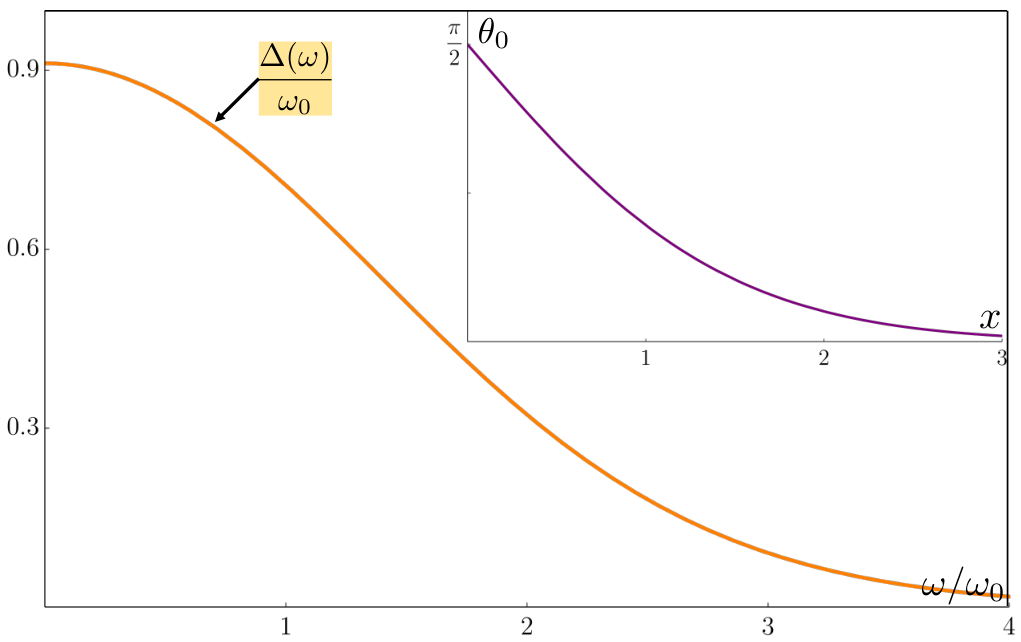
Recall from Sec. IV.2 that . Further, the requirement discussed in the beginning of Sec. III together with Eqs. (14) and (15) imply for Therefore, for we have
| (59) |
In the Appendix, we show that under the conditions (59) there exists a unique solution of the nonlinear differential equation (57) and note that is real analytic on the entire -axis by standard theorems of the theory of ODEs. This is a parameterless function which we plot in the inset to Fig. 4 for . Observe also that since leaves Eq. (57) invariant and by uniqueness, must map into itself under this transformation, i.e., .
Having determined , we know the gap function for all low temperatures, , and . Indeed, Eq. (15) implies
| (60) |
[Recall that we extended to defined on the entire real axis in Sec. IV.2.] This equation provides the leading small asymptotic behavior of for any and . Graphically, plots of the gap function vs. Matsubara frequency for any and tend to the same universal curve shown in Fig. 4 as , when both and are measured in units of .
It is straightforward to work out the expansion of at small and its large asymptote. Both depend on a single constant that needs to be determined numerically. At large , the angle is small and . Equation (57) becomes the Airy equation. Its solution that goes to zero at infinity is the Airy function of the first kind, . Therefore at large
| (61) |
where we determined the constant of proportionality 4.58 numerically and used the known asymptotic expansion for stegun.
Similarly, at small
| (62) |
In particular, recalling the definition (58) of , we find
| (63) |
Since this result is for , diverges as for andrey_ratio. For fixed and we have
| (64) |
where we took the value of for from Table 1. Reference andrey_ratio found the same answer, but for and with a prefactor instead of 8.47. Note that unlike in the BCS theory, here is not the gap in the spectrum notgap.
IX.2 Low free energy and specific heat
To evaluate the free energy , we use Eq. (27). As discussed in Sec. VIII, the free energy contains a diverging -independent constant because we took the limit . This divergence is present for superconducting states as well, since in these states when , same as in the normal state. To isolate it, we subtract and add the noninteracting part of the normal state free energy given by Eq. (48), i.e., . The difference is finite and we have already evaluated the dependence of in Sec. VIII.
Taking the difference , where , corresponds to the replacement in the Zeeman term in Eq. (27), since in the normal state. Using also , , and the symmetry property (16) of , we obtain the non-dimensionalized free energy in the superconducting state at as
| (65) |
Substituting the numerical solution for discussed in the previous subsection into the integral, we find
| (66) |
The specific heat in the superconducting state is
| (67) |
where
| (68) |
It is evident that becomes negative as for any .
This indicates that the model is pathological for just as it is above , see the discussion at the end of Sec. VIII. Again, there cannot be an unambiguous explanation of this pathology without the knowledge of the system Hamiltonian. To fix it, we need to modify the effective fermionic action (9), i.e., the model itself. One scenario is as follows. Consider the difference between and the normal state specific heat (54) ,
| (69) |
This is positive for . A straightforward numerical analysis shows that . Therefore, this difference is always positive when . Suppose the modification of the fermionic action is such that it introduces a new order parameter independent of . Further, suppose this adds terms to that depend on the new order parameter and not on [see Eqs. (11) and (12)]. Then, it does not affect the superconducting transition and the gap equation, but adds -dependent terms to the free energy and to the specific heat. The change in the specific heat must be the same for and . Provided the new is positive, so is the new , because Eq. (69) remains valid. This scenario is favorable for the results of this section in the sense that it fixes the pathology while leaving them intact with the exception of the answers for and . However, note that and do not change.
IX.3 Accuracy of the local approximation
In this section, we solved the gap equation on the Matsubara axis and evaluated the specific heat at low temperatures for , by replacing the gap equation (17), which we copy here for convenience,
| (70) |
with the differential equation (57). Now let us investigate the accuracy of this local approximation.
To derive Eq. (57), we expanded in to second order, see Eq. (24). The contribution from odd powers of to the right hand side of Eq. (70) cancels after summation over . Therefore, the error comes from terms of order 4 and higher. The Lagrange error bound then gives an upper bound on the difference between and our approximation to it. Here is the maximum value of .
Let us split the summation in Eq. (70) into two parts: and , where is to be determined. For we use the Taylor series expansion of to third order plus the Lagrange error bound. For , we replace , which provides an upper bound for the error from neglecting these terms. Pulling out an overall factor of , we obtain
| (71) |
The first term leads to Eq. (57) after the change of variables (58). The remaining three terms are the error. To estimate the second derivative of and , we use the numerical solution of Eq. (57) plotted in Fig. 4. For example, with and . We replace the summations over in Eq. (71) with integrals and then minimize the error with respect to . As turns out to be large, corrections due to the replacement of the summations with integrals are negligible. In this way, we obtain that the relative error [magnitude of the ratio of the sum of the last three terms in Eq. (71) to the first term] is
| (72) |
X Conclusions
In this paper, we studied the thermodynamics of a system of fermions near a quantum critical point with extremely retarded interactions of the form , where is a bosonic Matsubara frequency. The case of this model corresponds to the strong coupling limit of the Eliashberg theory, which is intermediately retarded. Extreme retardation at generic kicks in for and for at . Note that for , the model is a model without a Hamiltonian and is defined through a nonlocal effective Euclidian action only.
The model shows two phases: normal and superconducting. Similarly to the Eliashberg theory, the order parameter is the frequency dependent gap function , where is the fermionic Matsubara frequency. We determined the superconducting transition temperature and the order parameter near . The amplitude of serves as the Landau order parameter. We expanded the free energy functional to order near the transition to obtain the Landau free energy, from which we derived the jump in the specific heat and the thermodynamic critical field. These answers are asymptotically exact in the limit . We also evaluated the normal state specific heat for arbitrary and .
Next, we turned our attention to the properties of the model at low temperatures. We proved that the global minimum of the free energy is unique (nondegenerate). We derived the universal gap equation, which is a parameterless second order ODE, and determined the scaling of with , , and for all , , and . Building on this, we obtained explicit expressions for the free energy and specific heat in the superconducting state for this range of parameters. We also evaluated and found that it is finite for and , but diverges as for and as for . These results are exact for any at .
Note that “exact” and “asymptotically exact” here and elsewhere in this paper mean exact for the model defined by the effective action (9) in the thermodynamic and limits. In this regime, fluctuational corrections to the spin chain are negligible and it is at zero effective temperature, i.e., its ground state [which is determined by the gap equation (17)] captures all thermodynamical properties that we evaluated.
We found that the model is thermodynamically unstable for . Its specific heat is negative above for and also at for . We saw in an earlier paper breakEli that when this model is understood as an effective description of the phonon mediated electron-electron interaction (), this instability implies the emergence of a new order above . The new phase breaks the lattice translational symmetry and invalidates the model at least in a certain temperature range. For other , a microscopic Hamiltonian is similarly necessary to resolve this issue. An interesting open problem is therefore to construct classes of physical many-body Hamiltonians that correspond to the model with arbitrary .
Acknowledgements.
We thank Ar. Abanov, A. V. Chubukov, G. Kotliar, and T.-H. Lee for helpful discussions.*
Appendix A Existence and uniqueness of solutions to the universal gap equation
In this appendix we show that under the conditions (59) the universal gap equation (57) has a unique solution. Uniqueness is easier to show than existence, so we start with uniqueness, then discuss existence of a solution. We also offer a section about the properties of solutions of Eq. (57) when conditions (59) are dropped.
A.1 Uniqueness of a solution satisfying conditions (59)
Suppose that both and are twice continuously differentiable solutions of the ODE (57) that satisfy the conditions (59). Then vanishes when from the right, and when . Moreover, is also twice continuously differentiable, and its second derivative is given by
| (73) |
We multiply Eq. (73) by , integrate from to , integrate by parts on the left-hand side, and obtain
| (74) |
where the prime denotes derivative with respect to . The second inequality in (74) follows from the fact that is an increasing function for . Since both inequalities in (74) are strict if for some (and therefore in some open neighborhood of ), the only option compatible with (74) is: for all .
Thus uniqueness holds.
A.2 Existence of a solution satisfying conditions (59)
The uniqueness proof only shows that there cannot exist more than one twice continuously differentiable solution to Eq. (57) that satisfies the conditions (59), while leaving open whether a solution exists at all. In this subsection we show that such a solution does exist, indeed.
We now consider the initial value problem for Eq. (57), with initial data
| (75) |
and we treat as a real parameter that we exhibit explicitly in the solution to the initial value problem, written as . Our goal is to show that there exists at least one particular value (possibly not unique, in this section) such that the pertinent solution of the initial value problem satisfies the remaining conditions in (59); i.e., vanishes as , and takes values only in for . In this case we may identify with a sought-after solution of Eq. (57) under the conditions (59).
We begin by noting that the Picard-Lindelöf theorem Kamke guarantees that for each the initial value problem for Eq. (57) with initial data (75) has a unique twice continuously differentiable solution , which exists for all . The regularity follows from the facts that the function is continuous in both and . The uniqueness and global character of such a solution follow from the additional feature that the derivative of is uniformly bounded in absolute value. In fact, is analytic in ; this follows from the fact that the function is analytic in both and ; see Ref. davis. Thus it remains to show that there is a solution that converges to 0 as , and that this solution does not take values outside of the interval when .
Since we demand that the solution , with , it now follows from Eq. (57) that a necessary condition for the existence of such a solution is that the initial slope . Indeed, for and , the right-hand side of Eq. (57) is , so that the unique solution of Eq. (57) that satisfies the initial data (75) is convex as long as . But this means that if there is any for which and , then is a local minimum point of , and this solution will inevitably increase to values .
On the other hand, since we also demand that the solution , its negative initial slope cannot be too large in magnitude, for it is straightforward to show that there is some such that for there is an such that the pertinent solution satisfies and . (We have recycled the symbol with a new meaning.) In this case it follows right away that for some . To see that there is such an , recall that , so that we obtain the estimate
| (76) |
and integrating this estimate twice for the stipulated initial data we find that
| (77) |
The cubic polynomial at the right-hand side may have no, or one, or two positive roots, depending on . If there is at least one positive root, let denote either the unique positive root or the smaller of the two positive roots. Such a root exists if and only if . Setting , our cubic problem becomes , viz. which returns
| (78) |
And so, when the cubic upper bound to the solution of our initial value problem, i.e., Eq. (57) with initial conditions (75), vanishes at with a slope . Hence, itself must have a zero at some when . Moreover, . For suppose ; then both and its first derivative would vanish at , and by the uniqueness of the solution of the second-order initial value problem formulated with these data at , the function would have to vanish identically, which is a contradiction to the fact that . So , and since , it follows that , which violates the required lower bound 0 for . It follows that there is some with such that a further necessary condition for the existence of the desired solution is that the initial slope .
Now consider what happens to if we start with and continuously increase from there. As just discussed, the solution to the initial value problem (57), (75) has a smallest positive zero at , and . Moreover, for all Indeed, if there was some with , then , and as discussed above, would be a local minimum point of . This solution would increase for to values – in contradiction to the cubic upper bound we derived. Thus decreases monotonically from the value at to the value 0 at . Now increase continuously above . It is easy to see [just formally integrate Eq. (57) twice, using Eq. (75)] that for all one has and . Thus the zero moves continuously to the right as increases. Moreover, as long as , the function reaches its first zero at with a nonzero negative slope, . This follows from the already made observation that must be identically zero if it vanishes at a finite location with vanishing slope, in contradiction to the initial data . Thus we can increase until a value is reached at which , with (limit from the left). The solution is a sought-after solution .
A.3 The types of solutions for general initial data
We briefly discuss the general initial value problem for Eq. (57) with initial data at . By the -periodicity of the sine function, it suffices to restrict the discussion to data
| (79) |
For any pair of such initial data there exists a unique analytical solution of Eq. (57) for all ; cf. davis. The purpose of this subsection is to present a mostly qualitative and partly quantitative overview of the behavior of these solutions.
To get a more intuitive grasp of the possible solutions it is helpful to note that for the variable transformation
| (80) |
changes Eq. (57) into
| (81) |
for Here we have introduced Newton’s dot notation to denote derivatives with respect to . Equation (81) describes a damped rigid pendulum, or, equivalently, a point mass moving on an upright circle subject to uniform gravity and Newtonian friction, with a friction coefficient inversely proportional to time noworries. We count the angle from the “up” position, i.e., corresponds to the unstable inverted pendulum equilibrium and to the stable equilibrium. Of course, a priori any integer multiple of may be added to either or to obtain yet another unstable, respectively stable equilibrium solution for Eq. (81), because Eq. (81) in itself does not restrict to lie in any particular interval such as .
The damped pendulum Eq. (81) intuitively suggests that the damping will force the evolution of to converge at to one of the infinitely many copies of the two possible equilibrium states. Most initial data would lead to a (copy of the) stable equilibrium state . However, for each there should be a discrete set of slopes which launch a solution that asymptotically approaches (a copy of) the unstable equilibrium state . The approach to any stable equilibrium is damped oscillatory, while the approach to an unstable equilibrium is monotonic. Copies of the stable pendulum equilibrium have Newtonian energy and the copies of the unstable one .
There is one caveat to what we just wrote. Since the friction coefficient vanishes as , it is in principle conceivable that there also exist solutions that asymptotically approach a dynamical solution of the undamped pendulum equation, instead of converging to an equilibrium solution. We can rigorously rule out an asymptotic approach to a so-called librating solution of the undamped pendulum equation (see below), but we have not rigorously ruled out an asymptotic approach to an oscillating undamped pendulum solution; we expect that it does not occur, though.
In addition to these intuitive insights into the possible types of solution, we offer some exact results.
First, one can show the convergence of the Newtonian energy of the pendulum evolution
| (82) |
The energy is monotonically decreasing with due to friction. Indeed,
| (83) |
and for any the right-hand side in Eq. (83) is “” if . Since is bounded below, it must converge as . However, it may or may not converge to its minimum value .
We remark that convergence of to a constant as does not in itself imply convergence of as . After all, in the absence of friction the energy is conserved, hence trivially converges to a constant. At the same time, keeps oscillating or librating forever in this case, unless is one of the two equilibrium states. With the help of our energy dissipation identity (83) we can rule out an asymptotic approach to a librating solution, though. Namely, since , we can extract from Eq. (83) the two-sided bounds
| (84) |
with and some positive constants. Since any asymptotically librating solution has energy for some , it follows from the upper bound in Eq. (84) that the only possibilities are the asymptotic approach to the stable equilibrium (), to the unstable one (, or to an undamped oscillating pendulum solution ().
Second, whenever does converge to one of the equilibrium points of the damped rigid pendulum, i.e., to a zero of , linearization about that equilibrium yields an accurate approximation at large . Letting denote the deviation of from the equilibrium point, and dropping terms nonlinear in , we find that is (asymptotically) a solution of one of the following two ODEs, viz.,
| (85) |
These are Bessel differential equations. Their solutions for positive map into the Airy function in the original variables. More precisely, for large enough the function approaches the asymptotic form Ai. The constant is an integer multiple of , and the “” sign is to be chosen when an unstable pendulum equilibrium is approached monotonically, while the “” sign pertains to the oscillatory approach to a stable pendulum equilibrium. The constants , , and depend on the initial data.
References
- (1) D. Broun, What lies beneath the dome?, Nat. Phys. 4, 170 (2008).
- (2) T. Shibauchi, A. Carrington, and Y. Matsuda, A Quantum Critical Point Lying Beneath the Superconducting Dome in Iron Pnictides, Annu. Rev. Condens. Matter Phys. 5, 113 (2014).
- (3) G. Stewart, Heavy-fermion systems, Rev. Mod. Phys. 56, 755 (1984).
- (4) H. Wang, S. Raghu, and G. Torroba, Non-Fermi-liquid superconductivity: Eliashberg approach versus the renormalization group, Phys. Rev. B 95, 165137 (2017).
- (5) H. v. Löhneysen, A. Rosch, M. Vojta, and P. Wölfle, Fermi-liquid instabilities at magnetic quantum phase transitions, Rev. Mod. Phys. 79, 1015 (2007).
- (6) A. V. Chubukov, A. Abanov, Y. Wang, Y.-M. Wu, The interplay between superconductivity and non-Fermi liquid at a quantum-critical point in a metal, Ann. Phys. 417 168142 (2020).
- (7) J.P. Carbotte, Properties of boson-exchange superconductors, Rev. Mod. Phys. 62, 1027 (1990).
- (8) R. Combescot, Strong-coupling limit of Eliashberg theory, Phys. Rev. B 51, 11625 (1995).
- (9) E. A. Yuzbashyan and B. L. Altshuler, Migdal-Eliashberg theory as a classical spin chain, Phys. Rev. B 106, 014512 (2022).
- (10) Y. Wang, A. Abanov, B. L. Altshuler, E. A. Yuzbashyan, and A. V. Chubukov, Superconductivity near a Quantum-Critical Point: The Special Role of the First Matsubara Frequency, Phys. Rev. Lett. 117, 157001 (2016).
- (11) L. D. Landau and E. M. Lifshitz, Statistical Physics, Part 1, 3rd ed. (Butterworth-Heinemann, Oxford, 1980).
- (12) and , where or , couple to and , respectively, see Ref. spinchain for more detail.
- (13) E. A. Yuzbashyan and B. L. Altshuler, Fluctuations in boson-mediated superconductors and the meaning of the Migdal theorem (tentative title), unpublished.
- (14) This derivation of the spin chain holds everywhere in the configuration space (not only at the stationary points) when . A different derivation is available for general . See Secs. II and VII in Ref. spinchain.
- (15) To be more precise, taken at its minimum is the grand potential per volume as we work at fixed chemical potential. Nevertheless, we colloquially refer to it as the free energy or free energy density.
- (16) Here we do not consider the spin-flip saddle points spinchain where the sign of the right hand sides of Eqs. (13) flips for certain .
- (17) Cf. Eq. (18) and observe that an infinitely differentiable exists for the normal state at any finite as well. However, in this case changes abruptly from to 0 near for small and dropping higher order derivatives in Eq. (24) is not justified. In this way, the boundary condition eliminates the normal state as a solution of Eq. (25).
- (18) Not to be confused with the real frequency axis for the original complex frequency . In terms of , Matsubara frequencies correspond to discrete points on the imaginary axis and the “real axis” – to imaginary axis, .
- (19) R. A. Barankov, L. S. Levitov, and B. Z. Spivak, Collective Rabi Oscillations and Solitons in a Time-Dependent BCS Pairing Problem, Phys. Rev. Lett. 93, 160401 (2004).
- (20) E. A. Yuzbashyan, O. Tsyplyatyev and B. L. Altshuler, Relaxation and Persistent Oscillations of the Order Parameter in Fermionic Condensates, Phys. Rev. Lett. 96, 097005 (2006).
- (21) R. A. Barankov and L. S. Levitov, Synchronization in the BCS Pairing Dynamics as a Critical Phenomenon Phys. Rev. Lett. 96, 230403.
- (22) R. A. Barankov and L. S. Levitov, Excitation of the dissipationless Higgs mode in a fermionic condensate, arXiv:0704.1292 (2007).
- (23) E. A. Yuzbashyan, M. Dzero, V. Gurarie, and M. S. Foster, Quantum quench phase diagrams of an -wave BCS-BEC condensate, Phys. Rev. A 91, 033628 (2015).
- (24) E. A. Yuzbashyan and O. Tsyplyatyev, Dynamics of emergent Cooper pairing at finite temperatures, Phys. Rev. B 79, 132504 (2009).
- (25) At any finite , spins approach their normal state positions when , because in these limits, see Eq. (13). For we impose this as boundary conditions at infinity.
- (26) Consider that changes slowly with . The interaction part of the free energy (22) is then proportional to , where . The Zeeman term is negligible at any finite . The interaction is to be minimized subject to the constraint . Take for and otherwise. This satisfies the constraint and it is also clear that the interaction attains its absolute minimum when .
- (27) G. Grosso, G. P. Parravicini, Solid State Physics, 2nd ed. (Elsevier, Amsterdam, 2013).
- (28) H. Kleinert, Path Integrals in Quantum Mechanics, Statistics, Polymer Physics, and Financial Markets (World Scientific, Singapore, 2009).
- (29) As , we have and .
- (30) E. A. Yuzbashyan and B. L. Altshuler, Breakdown of the Migdal-Eliashberg theory and a theory of lattice-fermionic superfluidity, Phys. Rev. B 106, 054518 (2022).
- (31) M. Abramowitz and I. A. Stegun, Handbook of Mathematical Functions With Formulas, Graphs, and Mathematical Tables (U.S. Government Printing Office, Washington, D.C., 10th Printing, 1972), p. 448, Eqs. 10.4.59 and 10.4.61.
- (32) Y.-M. Wu, A. Abanov, A. V. Chubukov, Pairing in quantum-critical systems: Transition temperature, pairing gap, and their ratio, Phys. Rev. B 99, 014502 (2019).
- (33) The spectral gap is twice the solution of the equation on the real axis.
- (34) G. Teschl, Ordinary Differential Equations and Dynamical Systems (American Mathematical Society, Providence, Rhode Island, 2012).
- (35) H.T. Davis, Introduction to Nonlinear Differential and Integral Equations, 1st ed. (Dover Publications, New York, 1962).
- (36) There is no complication at due to this -dependent damping term because we already know that the initial value problem is well-defined in the variable at . It is therefore sufficient to consider the problem in the variable with data at some