A study of the local dynamics of modified Patankar DeC and higher order modified Patankar–RK methodsThanks: \monthyeardateAugust 11, 2026\correspondingPhilipp Öfffner
Abstract
Patankar schemes have attracted increasing interest in recent years because they preserve the positivity of the analytical solution of a production-destruction system (PDS) irrespective of the chosen time step size. Although they are now of great interest, for a long time it was not clear what stability properties such schemes have. Recently a new stability approach based on Lyapunov stability with an extension of the center manifold theorem has been proposed to study the stability properties of positivity-preserving time integrators. In this work, we study the stability properties of the classical modified Patankar–Runge–Kutta schemes (MPRK) and the modified Patankar Deferred Correction (MPDeC) approaches. We prove that most of the considered MPRK schemes are stable for any time step size and compute the stability function of MPDeC. We investigate its properties numerically revealing that also most MPDeC are stable irrespective of the chosen time step size. Finally, we verify our theoretical results with numerical simulations.
Funding.
This work was partially supported by the Deutsche Forschungsgemeinschaft (DFG) through grant ME 1889/10-1 (Izgin) and the Gutenberg Research College, JGU Mainz (Öffner).1 Introduction
The derivation of structure preserving methods is essentially important and has attracted much attention recently in various different ways, cf. [22, 18, 23, 2]. One specific family of schemes which ensures the positivity and conservation property of the numerical approximations are modified Patankar (MP) schemes. They are constructed for conservative and positive production-destruction systems (PDS) which are used to describe chemical reactions or biological models [4], but can also be found as the semi-discretization of convection equations (with and without) stiff source terms [6, 12]. Such a PDS is defined through the following system of ordinary differential equations (ODEs):
| (1) |
with , , and , where denotes the -th concentration, e. g. the density of a chemical or biological component. Further, the production rate denotes the rate of change from the -th component to the -th component whereas the destruction tells us the change from the -th component to the -th component.
The PDS is positive if the componentwise inequality implies for all . It is easy to see that due to , solutions of (1) fulfill additionally the conservation property for all .
To mimic conservation and positivity discretely, modified Patankar schemes have been first developed in [4] and further extended and applied in [18, 19, 21]. The proposed families of second- and third-order accurate modified Patankar–Runge–Kutta (MPRK) methods from [18, 19, 21] are based on explicit RK schemes. Huang and Shu have used as their starting point for the MP developments strong stability preserving (SSP) RK schemes in Shu-Osher form introducing SSPMPRK methods [11, 12]. However, all of those approaches have maximum order three, whereas arbitrary high-order MP schemes have later been proposed in [22]. These schemes are based on the Deferred Correction method [8]. All of those MP schemes are unconditionally positive and conservative for .
Although the benefits of MP schemes have been repeatedly demonstrated numerically since their introduction in 2003, an analytical study of their stability and robustness has been lacking until recently. In [27] some issues of MP schemes have been analyzed whereas in [13, 14, 15], a suitable stability theory for positivity-preserving time integration schemes has been proposed and applied to a family of second order MPRK schemes. In [10], this theory has been used to investigate the stability properties of the SSPMPRK schemes. In this paper, we follow the lines of [14, 15] and investigate the stability behavior of several MP schemes. We concentrate on the classical MPRK schemes from [18, 19] and the MPDeC approach up to order 14 [22].
The rest of the paper is organized as follows. In the next section, we shortly repeat the notation, the main definitions and results regarding the stability of fixed points from [15]. Next, in Section 3 and 4, we investigate the stability of MP schemes. First, we focus on a highly efficient MPRK scheme proposed in [27] and explain the general setting. Later, we consider the general families of third order MPRK schemes from [18, 19], denoted by MPRK43 and MPRK43. In Section 4, we extend our stability investigation to the MPDeC schemes from [22]. We want to mention here, that the resulting stability functions are included in our repository [17]. In numerical simulations, see Section 5, we verify our theoretical results. Finally, we formulate our conclusions and future research interests in section 6. In the Appendix 7, we give some additional material for completeness.
2 Preliminary Results and Notation
In the following part we shortly introduce the notation and the considered test equation where we also repeat the preliminary stability results for positivity-preserving schemes following [13, 14, 15].
2.1 Notation and Test Case
We consider a stable linear positive and conservative PDS of the form
| (2) |
with and the initial condition
| (3) |
following the notation and investigation in [10, 15]. In case that we have exactly linear invariants, there exist vectors which form a basis of the . As a consequence, they fulfill for all and . Note that for conservative PDS we find , i. e. the sum of each column vanishes, that is for . Due to a classical result from dynamical system theory [20], we know that (2) is positive if and only if is a Metzler matrix, i. e. the off-diagonal elements are nonnegative. Altogether, (2) can be rewritten as a positive and conservative PDS with and for and . Moreover,
| (4) |
holds true, which was already used in [10] to rewrite the SSPMPRK schemes in matrix-vector notation when applied to (2).
In what follows we are interested in comparing the stability properties of steady states of the initial value problem (2), (3) with those of the corresponding fixed points of the method. To that end, we recall the definition of (asymptotically) stable fixed points in the next section and refer to the analogue for steady states to [7, 25].
To ensure stable steady states , the matrix has a spectrum
and the eigenvalues of with zero real part have to be associated to a Jordan block size of 1, cf. [7, Theorem 2]. Also, according to the same theorem, no steady state of the test equation (2) is asymptotically stable since .
To summarize the assumptions on the linear PDS (2), we introduce the algebraic multiplicity of the eigenvalue as well as the corresponding geometric multiplicity . Altogether we consider in the following systems of the form
| (5) |
where denotes the diagonal of .
Remark 2.1.
We want to note, that and imply that the matrix is even a proper Metzler matrix, which means that in addition to being a Metzler matrix, possesses at least one negative diagonal element. As a result of [3, Theorem 10, Corollary 11], the only eigenvalue with is . Hence, the only eigenvalue for which we require equality of algebraic and geometric multiplicity in [7, Theorem 2] is .
As a final notation we want to introduce the diagonal matrix for a given vector by for .
2.2 Stability of Positive and Conservative Schemes
Here we recall the main theorem from [15] that we use for the subsequent stability investigation. The theorem provides sufficient conditions for the stability analysis of non-hyperbolic fixed points, i. e. fixed points of a map with , where the Jacobian of at possesses at least one eigenvalue with We consider the following stability notion of .
Definition 2.2.
Let be a fixed point of an iteration scheme , that is .
- 1.
is called Lyapunov stable if, for any , there exists a such that implies for all .
- 2.
If in addition to 1, there exists a constant such that implies for , we call asymptotically stable.
- 3.
A fixed point that is not Lyapunov stable is said to be unstable.
In the following we will also just speak of stable fixed points. A common result concerning the stability of fixed points is the following.
Theorem 2.3 ([25, Theorem 1.3.7]).
Let be an iteration scheme with fixed point . Suppose the Jacobian exists and denote its spectral radius by . Then
- 1.
is asymptotically stable if .
- 2.
is unstable if .
This theorem does not provide us with a criterion for the analysis of fixed points that are stable but not asymptotically stable, which must belong to the class of non-hyperbolic fixed points. Nevertheless, it gives a sufficient condition for detecting unstable fixed points. Still, the case of is not yet covered by Theorem 2.3, and thus, we use the following theorem from [15]. For a better reading flow we first introduce some notation.
Since we have assumed that the system has exactly linear invariants, there exist forming a basis of . Similar to [15], we introduce
as well as the set
| (6) |
and repeat the following theorem on the stability of an iteration in its explicit form, i. e. .
Theorem 2.4 ([15]).
Let such that represents a -dimensional subspace of with . Also, let be a fixed point of a map where contains a neighborhood of . Moreover, let any element of be a fixed point of and suppose that as well as that the first derivatives of are Lipschitz continuous on . Then for and the following statements hold.
- 1.
If the remaining eigenvalues of have absolute values smaller than , then is stable.
- 2.
We want to note that according to [10, Remark 2.4], is enough to conclude that has Lipschitz continuous derivatives for an appropriate neighborhood .
3 Stability investigation of modified Patankar schemes
In [14, 15], a novel stability investigation has been developed for conservative and positive time integration schemes. To that end, Theorem 2.4 was applied to a family of second order MPRK methods and it was shown that all fixed points are unconditional stable, i. e. stable for all . Recently, also families of SSPMPRK schemes have been investigated inside this framework [10]. In this section, we extend those investigations and consider modified Patankar schemes based on several Runge–Kutta methods. Thereby, the schemes are linearly implicit, so that the function satisfying is in all these cases implicitly given by solving linear systems. By the same reasoning as in [10], one can verify that for all schemes under consideration. The main idea for proving this is to show that the functions defined by the numerical scheme are in and that is obtained by solving only linear systems with a unique solution.
Similarly, all schemes preserve positive steady states with the same arguments as in [10] or [27, Prop. 2.3]. Thus, in order to apply Theorem 2.3 and part 1 of Theorem 2.4, we need to compute the eigenvalues of the Jacobian of evaluated at some steady state . However, to use also part 2 of Theorem 2.4, we need to prove that additionally conserves all linear invariants.
In order to compute we follow the approach as in [15, 10] introducing functions and several Jacobians. The functions arise from rearranging the equations for the stages of the numerical method leading to
| (7) | ||||
Note that is a function of vector-valued variables while depends on variables. As mentioned above, in all cases we will find are in , so that we may define
| (8) |
for with , and
| (9) |
for . Moreover, the operators indicate the evaluation of the corresponding Jacobian at et cetera, e. g. . As we interpret we also introduce the Jacobian
With that we can derive a formula for computing , where is the unique solution to (7). The chain rule yields
which can be rewritten to
| (10) | ||||
if all occurring inverses exist. Also, in order to avoid long formulas in the following, we may omit to write the functions together with all their arguments.
Stability of MPRK(3,2)
In [27] a novel three stage, second order MPRK method has been developed and investigated numerically. The scheme has shown favorable properties and is given by
| (11) | ||||
Note that this scheme is steady state preserving as the stages are uniquely determined and is a valid solution. Hence, writing we obtain .
Next, we apply MPRK(3,2) to (5) which, due to (4), yields in matrix vector notation the following identity
and we obtain
| (12) |
The second stage can be written as the linear system
| (13) |
This equation can be transformed using the fact that diagonal matrices commute and for all , yielding
| (14) | ||||
| (15) |
where as well as for and . Hence, we find
| (16) |
With analogous steps as before, the final step reads
| (17) |
Using again the above mentioned calculation rules, we get
| (18) | ||||
| (19) |
Therefore,
| (20) | ||||||
Since , we conclude that the inverses of the following matrices exist. We obtain from (10):
Hence, eigenvectors of are eigenvectors of the Jacobian . By substituting , we obtain the stability function for MPRK(3,2) with
| (21) |
so that
Before we analyze this stability function, we want to point out that, due to (18),
holds true for all as . Hence, the map generating the iterates of the MPRK(3,2) scheme conserves all linear invariants of the linear test problem. As a consequence, all conditions for applying Theorem 2.3 and Theorem 2.4 are met. It remains to prove that holds in order to conclude the stability of the fixed points as well as the local convergence towards the corresponding steady state solution satisfying for all .
Proposition 3.1.
The stability function satisfies and for .
Proof.
Obviously, it is . Then, we investigate for and . Elementary calculations yield for the denominator of :
where the numerator gives
Due to the even powers of , it is obviously that for , we have . Since is a rational function with poles11 1 Note that the stability function is always well defined on as otherwise a Jacobian of some must have been singular. at , we see that is holomorphic for all . We can apply the Phgramén-Lindelöf principle22 2 A special case of the principle is concerned with a holomorphic function on the interior of , which additionally is continuous on the imaginary axis and growths slower than the function for some and . For such a function it is possible to conclude for all if this inequality holds true on the imaginary axis [24, 26]. on the union of the origin and the interior of and deduce that for all . With the maximum principle, we know that is only possible on the imaginary axis since is not constant. Therefore, it follows for all with .
From this result, we can follow as a direct consequence of Theorem 2.4:
Corollary 3.2.
Remark 3.3.
We want to mention that as long as the stability function with polynomials satisfying and for all , we can conclude for whenever holds on the imaginary axis with the same reasoning as in the proof of Proposition 3.1.
Moreover, we point out that the Phragmén-Lindelöf principle can also be applied to different sectors of . Indeed, according to [3], all eigenvalues of a proper Metzler matrix with and lie in the sector . Hence, for investigating a scheme when applied to a system with at most four equations, it suffices to investigate the stability function on the boundary of rather than the imaginary axis. This approach might be useful to give first insights into the stability of a scheme whose analysis for the general case is more involved.
Stability of MPRK43()
In the following part, the third order accurate MPRK43-family from [18, 19] will be analyzed, which can be written as
| (22) | ||||
where and .
We want to note that in [18] the stages are labeled and , however, the first stage reads and can directly be inserted into the further stages. As a result, the first non-trivial stage is the second one, which we denote by here. As a result of this shift in superscript numbering, the stage corresponds to in our framework. We performed these changes in order to be consistent with our notation and to reduce the number of functions by one. Also note that by the same reasoning as above, this scheme is also steady state preserving so that yields for and .
The Butcher tableau with respect to the two parameters is defined by
| (23) |
with
| (24) |
and
We follow the steps from MPRK32 and obtain
The Jacobians of with respect to and are
| (25) |
For the second step, we obtain the linear system
| (26) |
In order to compute the Jacobians of with respect to and , we introduce
for some , where . We see that
| (27) | ||||
Hence, the derivatives of are given by the following terms, using :
| (28) | ||||
Next, satisfies
| (29) |
The derivatives are given by the following terms, using and (27):
| (30) | ||||
Finally, the last step can be written as
| (31) |
Note that from this equation we can conclude that the generating map conserves all linear invariants as implies Furthermore, the derivatives are given by the following terms, using :
| (32) | ||||
With the inverses needed for (10) exist and we get
| (33) | ||||
The stability function can be computed similar to the one of MPRK(3,2) and is given by
It can be reproduced in our repository [16], that this stability function can be rewritten in the form
| (34) |
where
An analytical investigation of the stability function of MPRK43() for arbitrary finite sized systems is outside the scope of this paper. This is due to the fact is a rational map in and and by expanding such that the coefficients of are polynomials in and , we see that the maximum total degree appearing in the numerator and denominator is . But it can be seen that is not true for all satisfying (24), see for instance Figure 1, where the stability region is highlighted in grey for .


Nevertheless, if we restrict ourselves to the case outlined in Remark 3.3, i. e. we investigate for systems with , we can prove that MPKR43() schemes are stable as we will find that on
Note that for the largest cone inside the stability region contains the sector , see Figure 1. Hence, to see the instability properties of MPRK43 numerically using a linear positive PDS (5), Theorem [3, Theorem 10] and a small calculation reveals that we would have to consider a proper Metzler matrix with .
Proposition 3.4.
Proof.
The following rather technical computations can be reproduced using our repository [16]. First, yields Next, we make use of Remark 3.3 and investigate on , i. e. we substitute with and . We obtain
Next, note that is equivalent to
| (36) | ||||
Dividing by and exploiting we have to prove that
The coefficients of can be written in terms of and resulting in
| (37) | ||||||
Let us consider , which is linear in . The coefficient of is a parabola in and vanishes for or Since for , the coefficient reads , we can conclude that the coefficient of is negative for all Now since , the biggest value of can be obtained for , resulting in
Additionally, we assumed that , so that on follows from Remark 3.3.
Remark 3.5.
We want to note that the assumption (35) of Proposition 3.4 can be easily verified for a given and . Indeed, it can be demonstrated that the assumption is always met for satisfying (24), however, an analytical proof is outside the scope of this paper. Instead we present 3D plots of (35) in the Appendix 7, see Figures 10 - 14.
From this result, we can follow as a direct consequence of Theorem 2.4:
Corollary 3.6.
- 1.
- 2.
Stability of MPRK43()
Already in [19] another MPRK43() has been proposed. It is based on
| (38) |
with The scheme reads
| (39) | ||||
where we again renamed the stages to be consistent with our framework. Moreover, the parameters above are given by
Following exactly the steps from before, we obtain for where
Note that again leads to proving that the scheme conserves all linear invariants. Furthermore, with solves so that also this scheme is steady state preserving for positive . Hence, we need to compute to apply Theorem 2.4 and Theorem 2.3. We get and which leads to
Next, using (27) we have
which determines but we omit to write it down here for a better reading flow. Furthermore,
Finally
The stability function is thus determined by (10) reading
| (40) | ||||
Note that the stability function is independent of the parameter , so that the following investigation is valid for all
Proposition 3.7.
Let be defined by (40). Then holds true for all and .
Proof.
A straightforward calculation yields
where
Hence and, additionally, we follow the proof of [10, Prop. 3.6], i. e. all we have to prove is that
for all . We denote by the above coefficient of . A small calculation reveals
which finishes the proof due to the even powers of .
From this result, we can follow as a direct consequence of Theorem 2.4:
4 Stability Investigation of modified Patankar Deferred Correction schemes
Arbitrarily high-order conservative and positive modified Patankar Deferred Correction schemes (MPDeC) were introduced in [22] which is based on the Deferred Correction approach developed in [8]. A time step is divided into subintervals, where and . The idea of the scheme is to mimic the Picard–Lindelöf theorem as follows. At each subtimestep and each correction step , an approximation is calculated. During each of the correction steps the approximation of the numerical solution is increased by one order of accuracy. The modified Patankar trick is introduced inside the basic scheme to guarantee positivity and conservation of the intermediate approximations. Using the fact that initial states are identical for any correction , the MPDeC correction steps can be rewritten for , and as
| (41) |
where are the correction weights and the index function is defined by
We also want to note that holds true for all by definition. The new numerical solution when applied to (5) is .
By means of an affine linear transformation of the interval to , the transformed subintervals are determined by . Then the correction weights can be computed according to the formula
where is the -th Lagrangian basis polynomials defined by the subtimenodes .
Due to the iterative correction process, MPDeC schemes are more complicated than the previous schemes, especially since the index function changes the weights of productive and destructive terms. Since depends on the sign of , we introduce the nonnegative part and nonpositive part . It is worth mentioning that
| (42) |
and
as well as . With that, we split the sum appearing in (41) into two sums containing and , respectively. For the separated sums, we know the value of so that we introduce the positive part
| (43) |
as well as the negative part given by
| (44) |
for , and . Using for and this can be rewritten as
| (45) |
Utilizing these vector fields, the iterates from (41) satisfy
| (46) | ||||
for and . Furthermore, analogously to the Jacobians introduced in (8) and (9), we write to represent the Jacobian with respect to the entries of the vector for some , evaluated at . Finally, we introduce similar notations for the Jacobians of and with respect to .
Also note that MPDeC schemes are steady state preserving as plugging in into (41) yields a true statement. Hence, for all and .
With that, we are able to compute for MPDeC schemes as the next theorem states.
Theorem 4.1.
Let , implicitly given by the solution of (46), be the generating map of the MPDeC iterates when applied to (5). Furthermore, let be a steady state of (5).
Then, and the Jacobian of evaluated at is given by
| (47) | ||||
for and . Thereby, is the Kronecker delta and
| (48) |
as well as
| (49) |
Proof.
Since the are fixed for a given scheme, the functions are in and as a consequence of solving only linear systems, the map is also in . Furthermore, the formula (47) follows analogously to (10), whereby we want to point out that the sum appearing in (47) is multiplied with for since in this case. Hence, we only have to prove the formulas (48) and (49). For this, we compute the Jacobians of each addend of the sums in (46) separately by considering (43) and (45).
Let us start proving (48), first considering . From (43) and for all it follows that
and hence, . Moreover, (45) for yields
Hence, using , we obtain
| (50) |
and for we find
Altogether, we obtain
| (51) |
and thus,
Next, for it follows from (43) that
Similarly, if . Furthermore,
yields
so that . This results in
proving (48).
To derive (49) consider first the case and . From (43) it follows immediately that
Moreover, (45) yields
which means that for . In total (46) gives us
Next, we investigate the case of and . Using and (43), we obtain
Furthermore, recalling (45), i. e.
we also distinguish between and . In the first case we see and
which means that . Turning to the case , we find
resulting in for . Altogether, we thus end up with
Finally, we have to consider the case and , i. e. we have to compute . Using and (43) once again we see that
Furthermore, we obtain
resulting in
With this, we have finally proven Theorem 4.1.
The distribution and number of the subtimesteps as well as the number of iterations determines the order of accuracy of the scheme. In the following, we will use equispaced and Gauss–Lobatto points. To reach order , we use corrections and subintervals for equispaced point distributions. Focusing on Gauss-Lobatto, a higher-order quadrature rule is applied33 3 The operator inside the DeC framework is based on a collocation method with Lobatto nodes (also known as the RK Lobatto III A method). . Here, we use M= ceil(K/2) subintervals and K=p corrections. We will denote the -th order MPDeC method by MPDeC. Note that MPDeC(1) is equivalent to the modified Patankar–Euler scheme and MPDeC(2) is equivalent to MPRK(2,2,1) investigated in [14]. Due to , MPDeC conserves all linear invariants, if for all since in this case the index function yields and (41) can be written as
which means that for all . Indeed, for equispaced nodes, with are the weights of the closed Newton–Cotes formulas for integrals over . Hence, a negative occurs for the first time at , i. e.with MPDeC. In this case, we also have to consider given in (44), resulting in
where we switched indices and used for the last equality. We observe that does not need to vanish for , so that the preservation of all linear invariants can not be guaranteed anymore for arbitrary systems (5) and MPDeC() with equispaced nodes and .
Moreover, in the case of Gauss–Lobatto nodes, the values for equal the weights of the corresponding Gauss-Lobatto quadrature, which are always positive. As a result, MPDeC with Gauss–Lobatto nodes conserve all linear invariants when applied to (5).
Remark 4.2.
From Theorem 4.1, we see that the Jacobian in general depends on , if there exist negative correction weights . For equispaced or Gauss–Lobatto points this is already the case for . Hence, to study the stability of MPDeC schemes applied to general linear systems, one needs to locate the eigenvalues of the Jacobian, which possibly depend on themselves. Such an analysis is outside the scope of this work, which is why we will focus on the following class of problems.
If is normal, then and share the same eigenvectors and the corresponding eigenvalues are the complex conjugate of each other. Since this means that even . Hence, we may discuss the stability of . Then, we find
for any rational maps , which means that the spectrum of the Jacobian of the map generating the MPDeC iterates can be written only in terms of the eigenvalues of . Using (47), (48) and (49), the stability function of MPDeC() for normal matrices and can be computed by
| (52) | ||||
for and . Note that if is symmetric it is also normal and we obtain , so that one can further simplify (52) to
| (53) | ||||
using . It is also worth mentioning that for the system matrix
| (54) |
with , used in [14, 27], we find that with , and thus
so that the stability function in this case is also given by (53).
Deferred Correction schemes are described by an iterative process which can be compared with classical RK schemes with more stages [1]. As MPDeC and DeC share the same amount of stages, we thus know that MPDeC(3) contains 5 stages using equispaced point distributions. Furthermore, MPDeC(4) has already 10 stages inside for equispaced points distributions, resulting in rational function with polynomial degree 10 in the numerator and denominator. Using Gauss-Lobatto nodes decreases the number of stages. For an MPDeC(4) we would end up with seven stages. By going even to arbitrary high-order the stability analysis would even become more complicated. Therefore, we avoid a theoretical analysis of the stability functions and investigate them numerically.
To give a first insight in the stability properties of MPDeC, we analyze the reduced stability function (53). In both cases described in Remark 4.2, the eigenvalues of leading to (53) are real, so that it is no loss of generality to restrict ourselves to the case with given in (54).
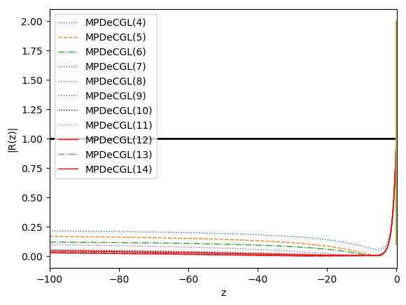
In Figure 2, we present the absolute value of the stability function over real . To obtain a stable scheme, the absolute value of has to be always smaller than one (the black line). In , we investigate MPDeC from order 4 to 14 using Gauss–Lobatto points. As can be recognized all MPDeC methods are stable using Gauss–Lobatto points. In , the stability functions of MPDeC schemes from 4th to 14th order are depicted for equispaced nodes. Here, we recognize that MPDeC(12) and MPDeC(14) are unstable but MPDeC(13) is stable. However, this is not surprising since already in classical DeC using equidistant points has been problematic for high-order methods, cf. [8, 9, 22, 27] and references therein. The reason for this is related with classical interpolation theory where it is known that equidistant points should be avoided. However, we would like to point out that our investigation supports as well the numerical investigation in [27] where problems in MPDeC-equidistant have been also recognized.

5 Numerical Experiments
In the following part, we verify the theoretical results of our considered modified Patankar schemes by numerical simulations. For the MPRK schemes we will consider more general systems where for the MPDeC schemes we restrict ourselves as described above to a system.
5.1 Numerical Simulations of MPRK Schemes
Due to our investigations in Section 3, all the considered MPRK schemes are unconditionally stable theoretically and our numerical experience will demonstrate this as well. For comparison, we will focus on the same tests as suggested and investigated in [14, 15, 10]. We consider the following three different settings:
- 1.
Test problem with exclusively real eigenvalues
- 2.
Test problem with complex eigenvalues
- 3.
Test problem with double zero eigenvalues
Test problem with exclusively real eigenvalues
As the first test, we consider the linear initial value problem (IVP)
| (55) |
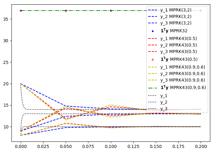
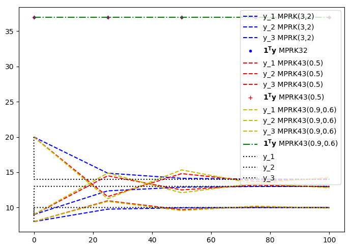
The IVP (55) has only positive off-diagonal elements inside the matrix and is therefore a Metzler matrix. Together with the positive initial values, this ensures that each component of the solution of the IVP is positive for all times. The eigenvalues are given by and and the analytical solution is given by
with . The steady state is given by The zero eigenvalue is simple and hence we obtain exactly one linear invariant given by . Therefore, the positive system is also conservative, e.g. for all . To demonstrate the stability of the MPRK methods, we select three different types focusing on MPRK32, MPRK43(0.5) and MPRK43(0.9,0.6). In Figure 3, the analytical and numerical results are shown. In 3(a), we plot it using to a comparably small time step of , whereas in 3(b) the time step is . In both cases our approximated solution converges towards the fixed point even for a big time step. Note that we still have oscillations except for the MPRK32 scheme, we refer again to [27] for a more detailed investigation on this topic.


Test problem with complex eigenvalues
The second test is the IVP
| (56) |
The system matrix in (56) is a Metzler matrix and we have the eigenvalues and . The analytical solution is given by
| (57) | ||||
and the steady state is . Also in this case a rapid decrease to can be expected through the behaviour of (57). In Figure 4, we see again the numerical solution compared to the analytical one. All schemes are stable and converge towards the steady state solution. The conservation property is ensured as well and can be recognized in 4(b).
Test problem with double zero eigenvalues
The third test is the linear IVP
| (58) |
The system matrix in (58) is a Metzler matrix with double zero eigenvalues . Therefore, we obtain besides (the conservative property), a second linear invariant with . Using the remaining eigenvalues and and corresponding eigenvectors, the analytical solution is given by
with . The steady state will be reached quite fast and it is given by . In Figures 5 and 6, we see the numerical results for our selected schemes for different . All schemes converge to the steady state solutions and preserve both linear invariants as presented in the figures.


5.2 Numerical Simulations of MPDeC Schemes
We consider the initial value problem
| (59) |
The nonzero eigenvalue and the analytical solutions is given by
The steady state is given by In Figure 7, the numerical and analytical solutions are plotted for several different MPDeC schemes.


From our investigation in Section 4, we know that using Gauss–Lobatto points leads always to stable and conservative approximations as can be also recognized in 7(a), however, for equidistant points, we obtain problems inside the approximation for higher-order approximations. This can also be seen in our numerical approximation for the IVP (59) in Figure 7(b). As we mentioned earlier this behaviour is not surprising since already the classical DeC method (without using the modified Patankar trick) has problems for high-order approximations, i. e. for -th order or higher, if equidistant points are used. Obviously, MPDeC(14) is unstable and alternates around the steady state solution. Nevertheless, we can obtain a stable discretization for this test case if we decrease the time step. We can estimate the time step using the eigenvalue and the value satisfying in Figure . From we thus find the bound . In Figure 8, we see an unstable behaviour for whereas for also MPDeC(14) converges to the steady state solution. Indeed, increasing up to to obtain stable approximations, however, the convergence rate will also be quite slow and we need more time to reach the steady state.


Note that the presented theory only claims a local convergence of the iterates towards the steady state. This can be seen, for instance, in the last example from [27, Figure B.9], where it is shown that the stable MPDeC(8) scheme does not convergence to the correct steady-state. Nevertheless, if we violate the stability condition, we can start arbitrary close to the steady state solution, and still, the iterates will not converge to . To clarify this, we change our IVP (59) to the following condition
| (60) |
In Figure 9, we plot the numerical solution calculated with order MPDeC(14) using equispaced points. The time step is selected with respect to the eigenvalue , so that holds. In 9(b), we see a slow convergence against the steady state. In Figures 9(c)-9(d), the conditions for convergence are not fulfilled and we see this also in our figures. A similar behaviour can be seen for analogously.


6 Conclusion
In this paper, we have investigated the stability conditions for several modified Patankar schemes. We were able to demonstrate that the MPRK(3,2) scheme proposed in [27] and the MPRK43() schemes from [18] are stable considering general positive linear systems. Further, we provided the stability functions for the MPRK43( schemes and investigated it for . For a fixed method, the conditions (35) can easily be checked whereas through a numerical study we have concluded that these conditions should be as well fulfilled for the general parameter selection. However, a formal proof is still missing. This remaining investigation will also be part of future research. We were also able to compute the stability function for MPDeC schemes and investigated the schemes numerically. We have seen that using Gauss–Lobatto points, we always obtain a stable scheme whereas for equispaced points stability issues have been recognized for higher-order methods and large . This fact is not surprising since already DeC methods show stability issues if equispaced points are used and also the investigation in [27] confirms those problems. We have seen that the bound can be estimated from stability functions and eigenvalues.
In the future, we plan to continue our investigation in several directions. First, we aim to investigate MPRK43() and MPDeC in more general setups. Furthermore, we will consider non-conservative Patankar systems as the ones proposed in [5]. Later, we combine MP schemes with proper selected space discretization and consider hyperbolic conservation/balance laws as it was already successfully done in [6]. However, it is not clear what the stability and convergence properties of such combined schemes are.
7 Appendix
We perform a numerical validation that Assumptions (35) are always fulfilled for the general parameter selection.


Acknowledgements
The author Th. Izgin gratefully acknowledges the financial support by the Deutsche Forschungsgemeinschaft (DFG) through grant ME 1889/10-1. P. Öffner was supported by the Gutenberg Research College, JGU Mainz. P. Öffner also wants to thank A. Meister (Kassel) for his invitation to Kassel.
References
- [1] R. Abgrall, É. Le Mélédo, P. Öffner, and D. Torlo, Relaxation deferred correction methods and their applications to residual distribution schemes, SMAI J. Comput. Math., 8 (2022), pp. 125–160, https://doi.org/10.5802/smai-jcm.82.
- [2] R. Abgrall, P. Öffner, and H. Ranocha, Reinterpretation and extension of entropy correction terms for residual distribution and discontinuous Galerkin schemes: application to structure preserving discretization, J. Comput. Phys., 453 (2022), p. 24, https://doi.org/10.1016/j.jcp.2022.110955. Id/No 110955.
- [3] L. Benvenuti and L. Farina, Eigenvalue regions for positive systems, Systems & Control Letters, 51 (2004), pp. 325–330, https://doi.org/https://doi.org/10.1016/j.sysconle.2003.09.009, https://www.sciencedirect.com/science/article/pii/S0167691103002846.
- [4] H. Burchard, E. Deleersnijder, and A. Meister, A high-order conservative Patankar-type discretisation for stiff systems of production–destruction equations, Appl. Numer. Math., 47 (2003), pp. 1–30, https://doi.org/10.1016/S0168-9274(03)00101-6.
- [5] A. Chertock, S. Cui, A. Kurganov, and T. Wu, Steady state and sign preserving semi-implicit Runge–Kutta methods for ODEs with stiff damping term, SIAM Journal on Numerical Analysis, 53 (2015), pp. 2008–2029, https://doi.org/10.1137/151005798.
- [6] M. Ciallella, L. Micalizzi, P. Öffner, and D. Torlo, An arbitrary high order and positivity preserving method for the shallow water equations, Comput. Fluids, 247 (2022), p. 21, https://doi.org/10.1016/j.compfluid.2022.105630. Id/No 105630.
- [7] P. Deuflhard and F. Bornemann, Scientific computing with ordinary differential equations. Transl. from the German by Werner C. Rheinboldt, vol. 42 of Texts Appl. Math., New York, NY: Springer, 2002.
- [8] A. Dutt, L. Greengard, and V. Rokhlin, Spectral deferred correction methods for ordinary differential equations, BIT, 40 (2000), pp. 241–266, https://doi.org/10.1023/A:1022338906936.
- [9] M. Han Veiga, P. Öffner, and D. Torlo, DeC and ADER: similarities, differences and a unified framework, J. Sci. Comput., 87 (2021), p. 35, https://doi.org/10.1007/s10915-020-01397-5. Id/No 2.
- [10] J. Huang, T. Izgin, S. Kopecz, A. Meister, and C.-W. Shu, On the stability of strong-stability-preserving modified Patankar–Runge–Kutta schemes, arxiv preprint arxiv:2205.01488, (202z2).
- [11] J. Huang and C.-W. Shu, Positivity-preserving time discretizations for production-destruction equations with applications to non-equilibrium flows, J. Sci. Comput., 78 (2019), pp. 1811–1839, https://doi.org/10.1007/s10915-018-0852-1.
- [12] J. Huang, W. Zhao, and C.-W. Shu, A third-order unconditionally positivity-preserving scheme for production-destruction equations with applications to non-equilibrium flows, J. Sci. Comput., 79 (2019), pp. 1015–1056, https://doi.org/10.1007/s10915-018-0881-9.
- [13] T. Izgin, S. Kopecz, and A. Meister, Recent developments in the field of modified Patankar-Runge-Kutta-methods, PAMM, 21 (2021), p. e202100027.
- [14] T. Izgin, S. Kopecz, and A. Meister, On lyapunov stability of positive and conservative time integrators and application to second order modified patankar-runge-kutta schemes, ESAIM: M2AN, 56 (2022), pp. 1053–1080, https://doi.org/10.1051/m2an/2022031, https://doi.org/10.1051/m2an/2022031.
- [15] T. Izgin, S. Kopecz, and A. Meister, On the stability of unconditionally positive and linear invariants preserving time integration schemes, SIAM Journal on Numerical Analysis, 60 (2022), pp. 3029–3051, https://doi.org/10.1137/22M1480318, https://doi.org/10.1137/22M1480318, https://arxiv.org/abs/https://doi.org/10.1137/22M1480318.
- [16] T. Izgin and P. Öffner, A study of the local dynamics of MPDeC and higher order MPRK methods (code). https://github.com/IzginThomas/MPRK43II.git, April 2023.
- [17] T. Izgin, P. Öffner, and D. Torlo, Modified Patankar: Oscillations and Lyapunov Stability (code). https://github.com/accdavlo/Modified-Patankar-Oscillations-and-Lyapunov-Stability, December 2022.
- [18] S. Kopecz and A. Meister, Unconditionally positive and conservative third order modified Patankar-Runge-Kutta discretizations of production-destruction systems, BIT, 58 (2018), pp. 691–728, https://doi.org/10.1007/s10543-018-0705-1.
- [19] S. Kopecz and A. Meister, On the existence of three-stage third-order modified Patankar-Runge-Kutta schemes, Numer. Algorithms, 81 (2019), pp. 1473–1484, https://doi.org/10.1007/s11075-019-00680-3.
- [20] D. G. Luenberger, Introduction to dynamic systems. Theory, models, and applications. New York etc.: John Wiley & Sons. XIV, 446 p. £ 10.50 (1979)., 1979.
- [21] A. Meister and S. Ortleb, On unconditionally positive implicit time integration for the DG scheme applied to shallow water flows, Int. J. Numer. Methods Fluids, 76 (2014), pp. 69–94, https://doi.org/10.1002/fld.3921.
- [22] P. Öffner and D. Torlo, Arbitrary high-order, conservative and positivity preserving Patankar-type deferred correction schemes, Appl. Numer. Math., 153 (2020), pp. 15–34, https://doi.org/10.1016/j.apnum.2020.01.025.
- [23] H. Ranocha, L. Lóczi, and D. I. Ketcheson, General relaxation methods for initial-value problems with application to multistep schemes, Numer. Math., 146 (2020), pp. 875–906, https://doi.org/10.1007/s00211-020-01158-4.
- [24] E. M. Stein and R. Shakarchi, Complex analysis, vol. 2 of Princeton Lectures in Analysis, Princeton University Press, Princeton, NJ, 2003.
- [25] A. Stuart and A. R. Humphries, Dynamical systems and numerical analysis, vol. 2, Cambridge University Press, 1998.
- [26] E. C. Titchmarsh, The theory of functions, Oxford University Press, Oxford, second ed., 1939.
- [27] D. Torlo, P. Öffner, and H. Ranocha, Issues with positivity-preserving Patankar-type schemes, Appl. Numer. Math., 182 (2022), pp. 117–147, https://doi.org/10.1016/j.apnum.2022.07.014.