Attacks on Perception-Based Control Systems: Modeling and Fundamental Limits
Abstract
We study the performance of perception-based control systems in the presence of attacks, and provide methods for modeling and analysis of their resiliency to stealthy attacks on both physical and perception-based sensing. Specifically, we consider a general setup with a nonlinear affine physical plant controlled with a perception-based controller that maps both the physical (e.g., IMUs) and perceptual (e.g., camera) sensing to the control input; the system is also equipped with a statistical or learning-based anomaly detector (AD). We model the attacks in the most general form, and introduce the notions of attack effectiveness and stealthiness independent of the used AD.
In such setting, we consider attacks with different levels of runtime knowledge about the plant. We find sufficient conditions for existence of stealthy effective attacks that force the plant into an unsafe region without being detected by any AD. We show that as the open-loop unstable plant dynamics diverges faster and the closed-loop system converges faster to an equilibrium point, the system is more vulnerable to effective stealthy attacks. Also, depending on runtime information available to the attacker, the probability of attack remaining stealthy can be arbitrarily close to one, if the attacker’s estimate of the plant’s state is arbitrarily close to the true state; when an accurate estimate of the plant state is not available, the stealthiness level depends on the control performance in attack-free operation.
I Introduction
The recent progress in deep-learning and computer vision has created a new generation of control systems that incorporate perceptual data for control and decision-making. For example, a camera or a light detection and ranging (LiDAR) sensor can provide the controller with information about plant states (e.g., distance to the obstacles, position in a local frame). Deep neural networks (DNNs) have shown capability to extract information from the complex perception data such as images.
Two main approaches – i.e., modular and end-to-end perception-based controllers have been recently developed [2]. With the end-to-end control approach, perception data (e.g., camera images, LiDAR 3D-point clouds), combined with other physical sensor information, is directly mapped to control inputs at runtime (e.g., see [3, 4, 5]). The controller is then either learned via supervised methods, such as imitation learning that mimics a pre-obtained optimal control input, or using deep-reinforcement learning techniques that design the control policy by maximizing the cumulative reward in an unsupervised fashion. On the other hand, with the modular control approach, a subset of state information is extracted from the perception data (e.g., images) and then combined with other physical sensor information, followed by the use of classic feedback controllers (e.g., [6, 7, 8]).
Despite the tremendous promise that DNN-based perception brings to controls, resiliency of perception-based controllers to well-documented adversarial threats remains a challenge, limiting their applicability in real-world scenarios. The main focus of adversarial machine learning methods has been on vulnerability of DNNs to small input perturbation, effectively focusing on robustness analysis of DNNs; e.g., targeting DNNs classification or control performance when a small and bounded noise is added to the images in camera-based control systems (e.g., [9, 10]). However, an attacker capable of compromising the system’s perception/sensing would not limit their actions (i.e., injected data) to small bounded measurement perturbation; the reason is that control theoretic methods for designing stealthy attacks suggests that the perturbation vector should gradually increase in size over time (e.g., [11, 12, 13, 14]).
Little consideration has been given on the potential impact of stealthy (i.e., undetectable) attacks, which are especially dangerous in the control context as many systems have recovery-based defenses triggered once an attack is detected. Model-based vulnerability analysis methods, designed from the control theory perspective, have been used to analyze the impact stealthy attacks could have on systems with linear time-invariant (LTI) dynamics and simple physical sensing, without perception, (e.g., [15, 16, 11, 14]). However, such analysis cannot be easily extended to systems with complex dynamics and sensing model that includes perception-based sensing.
Consequently, this work studies the impact that stealthy attacks on system sensing could have on perception-based control. We assume the attack goal is to move the system into an unsafe region while remaining stealthy from any anomaly detector (AD). Even though our notion of stealthiness is related to the work [17], we do not restrict the attack impact to the infinite time horizon. We show how such attacks can be modeled in a general form of an additive term for physical (i.e., non-perception) sensors and a generative model for perception sensors, without any assumptions about a bound on the perturbation values.
Perception-based controllers (either end-to-end or modular controllers) implicitly extract the state information from perception sensing (e.g., camera images) to derive suitable control inputs. Hence, the goal of this work is to evaluate their vulnerability to sensing attacks, by investigating whether there exist adversarial perception outputs that convey desired ‘falsified’ state information while remaining stealthy, rather than blindly adding noise or e.g., a patch to the current image. For example, for a vehicle with lane-keeping control (whose goal is to remain in the lane center), we find a sufficient stealthy attack sequence based on suitable adversarial image sequences conveying the desired falsified state information that is stealthy while fooling the controller into unsafe steering decisions.
Depending on attacker’s level of knowledge about the plant’s states, we derive conditions for which there exists a stealthy and effective (i.e., impactful) attack sequence that forces the system far from the operating point in the safe region. In particular, we assume that the attacker has full knowledge about the system’s open-loop dynamics, and consider two cases where at runtime the attacker (i) has or (ii) does not have access to the estimation of the plant’s state. We show that in the first case, the attack can approach arbitrarily close to the strict stealthiness condition as long as the estimation error is small. For the latter, the stealthiness level of the attack depends on the system’s performance in attack-free operation as well as the level of impact that the attacker expects to impose on the system (in terms of the distance from the system’s desired operating point due to the attack). Thus, there is a trade-off between the stealthiness guarantees and the performance degradation caused by the attack.
Moreover, for LTI plants, we show that these two cases fall in the same category, which means the attacker does not need to have access to an accurate estimate of the plant’s states. We also show that unlike in systems with LTI plants and linear controllers, where the design of stealthy and effective attacks is independent of the control design, for nonlinear plants the level of stealthiness is closely related to the level of closed-loop system stability – i.e., if the closed-loop system ‘is more stable’ (i.e., its trajectory converges faster to the equilibrium point), the attack can have stronger stealthiness guarantees. On the other hand, the attack impact (i.e., control degradation) fully depends on the level of open-loop system instability (e.g., the size of unstable eigenvalues for LTI systems).
I-A Related Work
The initial work [18] on adversarial example generation showed that DNNs are vulnerable to small input perturbations. Afterward, the majority of works has applied this idea to adversarial attacks on physical world such as malicious stickers on traffic signs to fool the detectors and/or classifiers [19, 20, 21]. For example, design of adversarial attacks for regression task has been studied in [22], where the goal of the attacker is to alter the geometrical prediction of the scene and the predicted distances from the camera. Yet, all these methods only consider classification or regression tasks in a static manner; i.e., the target only depends on its input, without consideration of the longitudinal (i.e., over time) system behaviours.
The vulnerability of perception-based vehicle controls has been recently studied in longitudinal way (e.g., [9, 10, 23, 24]). For instance, [9] considers autonomous vehicles with end-to-end DNN controllers that directly map perceptual inputs into the vehicle steering angle, and target the systems by painting black lines on the road. On the other hand, [23, 10] introduced online attacks on streams of images in the tracking task, while [24] considers longitudinal attacks on camera-LiDAR fusion. Specifically, [10] uses the idea of adding a small patch into the image for a couple of consecutive frames to change the position of the bounding box around each object, where the location and the size of the patch is obtained by solving an optimization problem.
However, these works only consider specific applications and analyze the attack impact in an ad-hoc manner, limiting the use of their results in other systems/domains. Further, they lack any consideration of attack stealthiness, as injecting e.g., adversarial patches that only maximises the disruptive impact on the control can be detected by most ADs. For instance, [25] introduced an AD that easily detects the adversarial attacks from [9]. On the other hand, in this work, we focus on systems with nonlinear system dynamics, define general notions of attack stealthiness, and introduce sufficient conditions for a perception-based control system to be vulnerable to effective yet stealthy perception and sensing attacks. We show that to launch a successful stealthy attack, the attacker may need to compromise other sensing information besides perception.
Finally, for non-perception control systems, stealthy attacks have been well-defined in e.g., [26, 11, 27, 16, 28, 17, 29, 30, 13, 31, 32, 33, 34], including replay [26], covert [28], zero-dynamic [27], and false data injection attacks [11, 12, 16]. However, all these work also only focus on LTI systems and linear controllers, as well as on specific AD design (e.g., detector). The problem of resilient state estimation for a class of nonlinear control systems has been considered in e.g., [35], focusing on systems that do not include perception as part of the closed-loop.
The notion of attack stealthiness independent of the employed AD (i.e., remaining stealthy for all existing/potential ADs) has been studied in [17]. We additionally differentiate our work in the following – our notion of stealthiness is stronger than the one in [17] as stealthiness there depends on time; i.e., there exists only a bounded time that the attack can stay undetected by an AD. However, the notion of stealthiness in our work is independent of time and the attack is guaranteed to be stealthy for all time steps after initiating the attack. Moreover, the performance degradation metric used in [17] is the error covariance of a Kalman filter estimator as opposed in our work; we assume the attacker’s goal is to force the system states into an unsafe region. In addition, we consider systems with nonlinear dynamics as well as with both perception and physical sensors, unlike [17] where only LTI plants with physical (i.e., without perception) sensors are investigated.
Further, this work considers attacks on both perception (e.g., images) and sensor measurements while the existing vulnerability analyses do not take into account perception. Besides, these works all assume LTI model and linear controller for the system dynamics while we consider a class of systems with nonlinear dynamical model and control. In addition, they focus on detectability of attacks with respect to specific detection schemes employed by the controller, such as the classic anomaly detection algorithm. Recently [30] has introduced a learning-based attack design for systems with nonlinear dynamics; yet, in addition to providing no formal analysis, the work only considers stealthiness with respect to the -based AD, and does not consider perception-based controllers.
I-B Paper Contribution and Organization
The contribution of this work is twofold. First, we consider attacks on perception-based control in the presence of ADs. We define a new notion of stealthiness using Neyman-Pearson Lemma and its relation with total variation and Kullback-Leibler (KL) divergence, where an attack is considered stealthy if it is stealthy from any AD. We find a sufficient condition for which the perception-based control systems are vulnerable to highly effective, in terms of moving the system from the desired operating point, yet stealthy attacks. Second, unlike all previous works in control literature, we consider highly impactful stealthy attacks on plants with nonlinear dynamics, controlled by a perception-based controller potentially employing an end-to-end nonlinear controller (e.g., DNN).
The paper is organized as follows. In Section III, we present the system model, as well as a model of attacks on perception before introducing the concept of stealthy yet effective attacks on the control systems. Section IV introduces two attack strategies and provides conditions under which the system is vulnerable to highly effective stealthy attacks. Finally, in Section V, we provide case studies to illustrate these conditions, before concluding remarks in Section VI.
II Preliminaries
In this section, we introduce employed notation before presenting properties of KL divergence known as data processing inequality, monotonicity and chain-rule as presented in [36].
Notation
denotes the set of reals, whereas and denote the probability and expectation of a random variable. For a square matrix , is the maximum eigenvalue. For a vector , denotes the -norm of ; when is not specified, the 2-norm is implied. For a vector sequence, denotes the set . A function is Lipschitz on the set with constant if for any it holds that ; it is globally Lipschitz with constant if . If and are two sets, includes the elements in that are not in . For a set , and define the boundary and the interior of the set, respectively. denotes a closed ball centered at zero with radius ; i.e., , whereas is the indicator function on a set . For a function , we denote as the partial derivative of with respect to and is the gradient of the function (-th element of the function ). Finally, if and are probability distributions relative to Lebesgue measure with densities and , respectively, then the total variation between them is defined as . The KL divergence between and is defined as .
Properties of KL Divergence and Other Preliminaries
In the following lemmas, and are assumed to be random variables (Lemmas 1-4 proofs can be found in [36]).
Lemma 1.
[Data Processing Inequality] Assume is produced given based on the conditional law . Let (respectively ) denote the distribution of when is distributed as (respectively ). Then
| (1) |
Lemma 2.
[Monotonicity] Let and be two distributions for a pair of variables and , and and be the marginal distributions for variable . Then,
| (2) |
Lemma 3.
[Chain rule] Let and be two distributions for a pair of variables and . Then,
| (3) |
where is defined as
| (4) |
Lemma 4.
Let and be two Gaussian distributions with the same covariance and different means and , respectively. Then, it holds that
| (5) |
Lemma 5.
Let be a distribution for a scalar random variable , and that for some . Then,
| (6) |
Proof.
The proof is straightforward from the definition of expectation and some properties of the integral. ∎
III Modeling Perception-Based Control Systems in the Presence of Attacks
In this section, we introduce the system model and show how to capture attacks on system sensing, including perception. Specifically, we consider the setup from Fig. 1 where each of the components is modeled as follows.
III-A Plant and Perception Model
We assume the plant has nonlinear dynamics in the standard state-space form
| (7) |
Here, , , , , and denote the state, input, system disturbance, observations from perception-based sensors, (non-perception) sensor measurements, and sensor noise, at time , respectively. The perception-based sensing is modeled by an unknown generative model , which is nonlinear and potentially high-dimensional. For example, consider a camera-based lane keeping system. Here, the observations are the captured images; the map generates the images based on the vehicle’s position. Without loss of generality, we assume that . Finally, the process and measurement noise vectors and are assumed independent and identically distributed (iid) Gaussian processes and .
III-B Control Unit
The control unit, shown in Fig. 1, consists of perception, controller, and anomaly detector units. We assume that the control unit receives and as the sensor measurements and perception sensing (e.g., images), respectively as an input. Thus, without malicious activity, it holds that and . Now, we describe in detail each of the components.
III-B1 Perception
We assume that there exists a perception map that imperfectly estimates the partial state information from from perception sensing (e.g., images) – i.e.,
| (8) |
here, denotes a deep neural network (DNN) trained using any supervised learning method on a data set collected densely around the operating point of the system, as in [37, 38]. In addition, is the perception map error that depends on the state of the system – i.e., smaller around the training data set. To capture perception guarantees, we employ the model for robust perception-based control from [6], and the standard model of the perception map (8) from [7] that can capture well DNN-based perception modules. Specifically, if the model is trained effectively, we assume that the perception error around the operating point is bounded, i.e., the following assumption from [7] holds.
Assumption 1.
There exists a safe set with the radius (i.e., ) around the operating point such that for all , it holds that , where – i.e., for all , . Without loss of generality, in this work, we consider the origin as the operating point – i.e., .

Remark 1.
As will be shown later in this work, the assumption on boundedness of and having a good estimate of such bound is only essential for the defender because the perception map is also used for anomaly detection. We should note that such bound will not be employed by the attacker to design stealthy impactful attacks. A systematic method to find the bound on is discussed in [7].
III-B2 Controller
The physical plant (7) is controlled by a (general) nonlinear controller that maps the image and physical sensor information to the input control. Using (7), one can write the above control law in an equivalent form of that absorbs in the control function . Hence, for
the evolution of the closed-loop system can be captured as
| (9) |
In the general form, the controller can employ any end-end control policy that uses the image and sensor measurements. For noiseless systems, the state dynamics can be captured as11 1 With slight abuse of notation, is used to denote the states of the noiseless system; yet, in the rest of the paper we use to denote the states of the actual physical system with noise and we clarify if the other case is implied.
| (10) |
Definition 1.
The origin of the system (10) is exponentially stable on a set if for any , there exist and , such that for all .
Lemma 6 ([39]).
For the system from (10), if there exists a function such that for any , the following holds
| (11) |
for some positive , and , then the origin is exponentially stable.
Assumption 2.
Remark 2.
The assumptions for closed-loop system are critical for system guarantees without the attack; i.e., if the system does not satisfy the stability property in attack-free scenarios, then an effective strategy for the attacker would be to wait until the system fails by itself. We refer the reader to the recent work e.g., [6, 7] on design of such controllers.
Remark 3.
Note that the exponential stability assumption on the closed-loop system (10) is only considered due to the simplicity of the notation and can be relaxed to control systems with asymptotic stability that satisfies the converse Lyapunov theorem conditions [40] (Theorem 3.14). Specifically, a similar result as in Lemma 8 can be obtained; however, the needed notation would be significantly more cumbersome.
Definition 2.
Let be the set of all functions such that the dynamics , where satisfies , reaches arbitrarily large states for some nonzero initial state . For a function from and an initial condition , we define
| (12) |
i.e., is the minimal number of time-steps needed for an unstable dynamic , starting from the initial condition , to leave a bounded ball with the center at zero and radius .22 2 To simplify our notation, and since we consider specific from the plant dynamics (7), we drop the the subscript .
III-B3 Anomaly Detector
The system is equipped with an anomaly detector (AD) designed to detect the presence of any abnormal behaviours. We use and to capture sensor (from (7)) and perception-based (from (8)) values without and under attack, respectively – we use the superscript to differentiate all signals of the attacked system, with the full attack model introduced in the next subsection.
Now, by denoting , we consider the classical binary hypothesis testing problem:
: normal condition (the AD receives );
: abnormal behaviour (the AD receives ).
Effectively, the AD uses both the extracted state information from the perception map (i.e., (8)) as well as sensor measurements. Given a random sequence , it either comes from the distribution (null hypothesis ), which is determined by system uncertainties, or from a distribution (the alternative hypothesis ); note that the unknown distribution is controlled by the attacker.
For a given AD specified by a function , two types of error may occur. Error type (), also referred as false alarm, occurs if when ; whereas type () error (miss detection) occurs if when . Hence, the sum of the conditional error probabilities of AD for a given random sequence is
| (13) |
Note that is not a probability measure as it can take values larger than one. Let us define as the probability of true detection, and as the probability of false alarm for the detector . We say that an AD (defined by ) to be better than a random guess-based AD (defined by ) if ; as with the random guess it holds that
III-C Attack Modeling
We assume that the attacker has the ability to compromise perception-based sensing (e.g., camera images) as well as (potentially) the sensor measurements delivered to the controller (see Fig. 1). Such attacks on physical sensors can be achieved by directly compromising the sensing (or the environment of the sensors) or the communication between the sensors and the controller [41, 42]. On the other hand, implementing the attack on the images delivered to the controller may not be feasible using physical spoofing attacks such as LiDAR spoofing by injecting laser data points [21, 24]. Hence, the attacker needs to compromise the images in cyber domain (e.g., as discussed in [43]). This can be achieved by modifying the firmware directly on the camera or the driver code, as done in Hyundai’s Gen5W and Tesla’s Model 3 attacks where custom firmware was installed [44, 45], or the Tesla Model S attacks that sent custom messages by compromising application drivers [46]. Similarly, such cyber attacks can be achieved using Man-in-the-Middle attacks that target the connection between the camera and the controller; examples include intercepting legitimate messages and manipulating their contents, before resending to the intended destination (e.g., as described in inter-vehicle attack scenarios in [41, 42] or vehicle attacks that manipulated timing on V2V/V2I messages, causing out-of-date situational awareness [47].
Moreover, we assume the attack starts at , and as previously mentioned, we use the superscript to differentiate all signals of the attacked system, for all ; the attack sequence is , where e.g., the value of observation delivered to the perception unit at time is denoted by . Note that due to nonlinearity of the operators ( and ), we do not employ the additive false-data injection model for perception attacks, widely used for LTI systems with non-perception sensing (e.g., [11]).
Thus, the system dynamics under attack can be modeled as
| (14) |
In this work, we assume the attacker has full knowledge of the system, its dynamics, and employed architecture. Further, the attacker has the required computation power to calculate suitable attack signals to inject, planning ahead as needed.
Remark 4.
The assumption that the attacker has knowledge of the system dynamics (i.e., function and matrix ) is commonly used in existing studies focused on the worst-case analysis of the attack impact on control systems [11, 12, 16, 14]. In particular, by focusing on resourceful attackers who possess extensive knowledge of the targeted systems, we can effectively assess the consequences of worst-case attacks and develop appropriate defensive strategies. However, the attacks presented in Section IV do not require knowledge of the noise profile, significantly improving their applicability.
Remark 5.
In our notation, denotes a state trajectory of the system under attack (for an attack starting at ), while denotes the state trajectory of the attack-free system; we refer to such state trajectory as the attack-free trajectory. Thus, when comparing the attack-free trajectory and the system trajectory under attack (i.e., from (14)), we assume that and . However, we cannot make such assumption for as it is a function of states and the states are compromised due to the attack.
We define an attack to be stealthy if the best strategy for the AD is to ignore the measurements and make a random guess between the hypotheses; i.e., that there is no AD that satisfies . However, reaching such stealthiness guarantees may not be possible in general. Therefore, we define the notion of -stealthiness, which as we will show later, is attainable for a large class of nonlinear systems. Formally, we define the notions of strict stealthiness and -stealthiness as follows.
Definition 3.
Consider the system defined in (7). An attack sequence is strictly stealthy if there exists no detector for which holds, for any . An attack is -stealthy if for a given , there exists no detector such that holds, for any .
Before introducing the sufficient condition for the above notion of stealthiness, we consider the following lemma.
Lemma 7.
The anomaly detector satisfies if and only if . Also, if and only if performs as a random-guess detector.
Proof.
Now, if we have , then we get where the decision of the detector is independent of the distribution of and therefore, the detector performs as the random guess detector. Since the reverse of all these implications hold, the other (i.e., necessary) conditions of the theorem also hold. ∎
Now, we can capture stealthiness conditions in terms of KL divergence of the corresponding distributions.
Theorem 1.
An attack sequence is strictly stealthy if and only if for all . An attack sequence is -stealthy if the corresponding observation sequence satisfies
| (16) |
Proof.
With some abuse of notation only specific to this theorem, and are used to denote and , respectively. First we prove the strictly stealthy case.
Using Neyman-Pearson lemma for any existing detector , it follows that
| (17) |
where the equality holds for the Likelihood Ratio function as [48]. Since , from [49] and the definition of total variation distance between and , it holds that
| (18) |
where denotes the total variation distance between the distributions.
Remark 6.
The -stealthiness condition defined in [17] requires that
This allows for the KL divergence to linearly increase over time for any , and as a result, after large-enough time period the attack may be detected even though it satisfies the definition of stealthiness from [17]. Yet, the -stealthiness from Definition 3 only depends on and is fixed for any time ; thus, it introduces a stronger notion of stealthiness for the attack.
Attack Goal
We capture the attacker’s goal as maximizing degradation of the control performance. Specifically, as we consider the origin as the desired operating point of the closed-loop system, the attack objective is to maximize the (norm of) states . Moreover, the attacker wants to remain stealthy – i.e., undetected by any employed AD, as formalized below.
Definition 4.
The attack sequence, denoted by is referred to -successful attack if there exists such that and the attack is -stealthy for all . When such a sequence exists for a system, the system is called -attackable. Finally, when the system is -attackable for arbitrarily large , the system is referred to as perfectly attackable.
In the rest of this work, our goal is to derive methods to capture the impact of stealthy attacks; specifically, in the next section we derive conditions for existence of a stealthy yet effective attack sequence resulting in for some – i.e., we find conditions for a system to be -attackable. Here, for an attack to be stealthy, we focus on the stealthy notion; i.e., that the best AD could only improve the probability detection by compared to random-guess baseline detector.
IV Conditions for -Attackable Systems
To provide sufficient conditions for a system to be -attackable, in this section, we introduce two methodologies to design attack sequences on perception and (classical) sensing data. The difference in these strategies is the level of information that the attacker has about the system; we show that the stronger attack impact can be achieved with the attacker having full knowledge of the system state.
Specifically, we start with the attack strategy where the attacker has access to the current estimation of state; in such case, we show that the stealthiness condition is less restrictive, simplifying design of -stealthy attacks. For the second attack strategy, we show that the attacker can launch the attack sequence with only knowing the function (i.e., plant model); however, achieving -stealthy attack in this case is harder as more restrictive conditions are imposed on the attacker.
IV-A Attack Strategy I: Using Estimate of the Plant State
Consider the attack sequence where and injected at time , for all , satisfy
| (19) |
with , and for a nonzero . Here, denotes an estimation of the plant’s state (in the presence of attacks), and thus is the corresponding state estimation error. Note that the attacker can obtain by e.g., running a local estimator using the true measurements before injecting the false values; i.e., and . We assume that the estimation error is bounded by – i.e., , for all .
On the other hand, the above attack design may not require access to the true plant state , since only the ‘shifted’ (i.e., ) outputs of the real sensing/perception are injected. For instance, in the lane centring control (i.e., keeping the vehicle between the lanes), only shifts the actual image to the right or left depending on the coordinate definition. Similarly, the attack on physical (i.e., non-perception) sensors can be implemented as where the attacker only needs to subtract from the current true measurements.
The idea behind the above attacks is to have the system believe that its (plant) state is equal to the state ; thus, referred to as the fake state. Note that effectively both and used by an AD are directly functions of the fake state . Thus, if the distribution of is close to (i.e., attack-free trajectory), then the attacker will be successful in injecting a stealthy attack sequence.
Definition 5.
For an attack-free state trajectory , and for any and , is the probability that the system state and physical sensor noise remain in the zero center ball with radius and , respectively, during time period , i.e.,
| (20) |
When the system with exponentially stable closed-loop control dynamics33 3 Note that under similar conditions the same analysis also holds for asymptotic stability condition [40] is affected by a bounded perturbation, one can show that the state of the system will remain in a bounded set. The following lemma from [40] provides the condition and the upper bound on the norm of the state.
Lemma 8 ([40]).
Let be an exponentially stable equilibrium point of the nominal system (10). Also, let be a Lyapunov function of the nominal system that satisfies (11) in , where . Suppose the system is affected by additive perturbation term that satisfies . If with holds for all and some positive , then for all , there exists such that for all holds with , and for it holds that with .
The next result captures conditions under which a perception-based control system is not resilient to attacks, in sense that it is (,)-attackable.
Theorem 2.
Consider the system (7) with closed-loop control as in Assumption 2. Assume that the functions , (derivative of ) and (derivative of ) are Lipschitz, with constants , and , respectively, and let us define , and for some . Moreover, assume that there exists such that the inequalities and , for some , are satisfied. Then, the system (7) is (,)-attackable with probability for some , if it holds that and with , and .
The theorem proof is provided in Appendix -A.
From (11), can be viewed as a ‘measure’ of the closed-loop system stability (larger means the system converges faster to the equilibrium point); on the other hand, from Theorem 2, closed-loop perception-based systems with larger are more vulnerable to stealthy attacks as the conditions of the theorem are easier to satisfy. However, if the plant’s dynamics is very unstable, is smaller for a fixed and . Thus, the probability of attack success is larger for a fixed and .
It should be further noted that , used in Theorem 2 conditions, would be equal to zero for LTI systems; thus, causing to become zero. Similarly when the mapping approaches more towards linear behaviour, will go to zero. Therefore, the inequality holds for linear systems and linear controllers. However, larger values of will help the inequality to be satisfied even for nonlinear control systems. In simulation results described in Section V, we discuss when these conditions are satisfied in more detail.
Moreover, in the extreme case when (i.e., the attacker can exactly estimate the plant state), the condition will be relaxed and the other condition becomes less restrictive as becomes smaller. Thus, in this case, if the attacker initiate the attack with arbitrarily small , then can be arbitrarily close to zero and the attack will be very close to being strictly stealthy. Hence, the following result holds.
Corollary 1.
Assume , with , and the functions , (derivative of ) and (derivative of ) are Lipschitz, with constants , and , respectively. If with , and holds, then the system (7) is (,)-attackable with probability , where for and some .
Finally, the above results depend on determining such that . Hence, the following result provides a sufficient condition for .
Proposition 1.
Let be a continuously differentiable function satisfying and define . Assume that , and for any it holds , where and are in class of functions [40]. Further, assume that can be chosen arbitrarily large. Now,
- •
if , then for any .
- •
However, if , then for any .
Proof.
We prove the first case and the second case can be shown in a similar way.
If , there exists a bounded ball with radius and center at zero (referred to as ) such that for all with it holds that . Since the function is differentiable, using the Mean-value theorem for the dynamics with and for any , we have that
| (21) |
Thus, for any , we have . Let us define where for any . Such minimum exists as the considered set is compact and we have in . Let us also assume . Now, we claim that the trajectories starting from should leave the set through the boundaries of .
To show this, we know that for any , , since . Then, for any
| (22) |
The above inequality shows that cannot stay in the set forever as is bounded on the compact set . On the other hand, cannot leave the set through the boundaries satisfying or the surface of because . Thus, the trajectories should leave the set through the surface of , and as can be chosen arbitrarily large, the trajectories of will diverge to becoming arbitrarily large. ∎
Example 1.
Consider the dynamical system
| (23) |
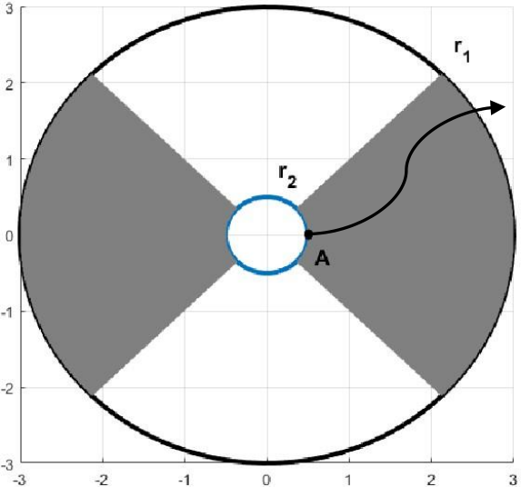
and let us consider the function . Hence, we have and
Since , for any , there exists such that for the dynamics with . The shaded region in Fig. 2 shows the area where outside and inside of . Moreover, any area outside of the ball satisfies (i.e., is increasing over time). Now, by denoting the state value at point with , we have . As ) is increasing outside as increases, any trajectory starting at cannot leave the shaded region from the surface of corresponding to or ; it also cannot stay in the region for all , as the trajectory evolves. Thus, the system states will eventually leave the shaded region, ‘exiting’ from the surface of the ball .
Theorem 2 provides conditions on the closed-loop system stability that may not hold in general for any system with closed-loop exponential stability. In the following theorem, we show that one can still obtain a similar (,)-successful attack (possibly with a larger ) even when the closed-loop system only satisfies exponential stability.
Theorem 3.
Proof.
Using the same definition as in (9) we have
From the Lipschitz property of function , it follows that , and with probability we have
Therefore, with probability it holds that for all .
Since the closed-loop system is exponentially stable, we use Lemma 8 to show that the dynamics will remain in a bounded ball centered at zero with such probability for all . The bound is obtained by . Using the Data-processing inequality of KL divergence and following the same procedure as in Theorem 2 we obtain
This means that the system is (,)-attackable with probability and . On the other hand, since we have with , similarly as in Theorem 2, we can show that for the states of the under-attack system will satisfy with probability . ∎
Note that our results only focus on the existence of perception measurements , obtained by shifting the current perception scene by , that results in -successful attack, and not how to compute it. Further, to derive attack sequence using Attack Strategy I, the attacker needs the estimation of the plant states. Thus, Attack Strategy II relaxes this assumption, with the attacker only needing to have knowledge about the plant’s (open-loop) dynamics and the computation power to calculate ahead of time.
IV-B Attack Strategy II: Using Plant Dynamics
Similarly to Attack Strategy I, consider the attack sequence where and , for all , satisfy
| (24) |
for some nonzero . However, here the attacker does not need an estimate of the plant’s state; they simply follow plant dynamics to find the desired measurements’ transformation. Now, we define the state as the fake state, and the attacker’s intention is to make the system believe that the plant state is equal to .
The following theorem captures the condition for which the system is not resilient to attack strategy II, in the sense that it is -successful attackable.
Theorem 4.
Consider the system (7) that satisfies Assumption 2. Assume that both functions and are Lipschitz, with constants and , respectively. Moreover, assume that there exists such that the inequalities and with are satisfied, where , and . Then, the system (7) is (,)-attackable with probability and , for some , if it holds that and .
The proof of the theorem is provided in Appendix -B.
Unlike in Theorem 2, and in Theorem 4 increase as increases. Therefore, unless , one cannot claim that the attack can be -stealthy for arbitrarily large as the inequality might not be satisfied. Therefore, there is a trade-off between the stealthiness guarantees () and the performance degradation caused by the attack (). However, in an extreme case where the system is linear, it holds that and ; before introducing the results for LTI systems in the next subsection, we remark on the following.
Remark 7.
The fact that we considered the control input in a general end-to-end form can help us verify that our results also hold when the perception-based control system is modular; i.e., when the states are extracted from the perception module and physical sensors and then used with the classic control methods. This is because the end-to-end formulation of the controller is very general, also covering the modular methods. In such case, the traditional control methods can be used such that the noiseless closed-loop system becomes exponentially or asymptotically stable.
IV-C Attack on LTI Systems
To derive sufficient conditions for which stealthy yet effective attacks exist, we have designed such attacks for perception-based control systems where plants have input affine nonlinear dynamics. However, for LTI plants, the obtained conditions can be significantly relaxed. Specifically, for LTI systems, because the system dynamics takes the form of , Attack Strategies I and II become identical as
| (25) |
Therefore, the attacker does not need to estimate the state of the system and they can use the Attack Strategy II to design the attack sequence.
In general, assume that for such systems we use the controller satisfying Assumption 2, where due to complexity of perception (e.g., image observations), a nonlinear function maps the perception sensing (e.g., the image) and sensors to the control input. Hence, from Corollary 1, we directly obtain the following result.
Corollary 2.
Consider an LTI perception-based control system with . Assume that with , , and the matrix is unstable. Then the system is (,)-attackable with probability , for arbitrarily large and , with and some .
Note that even though the above corollary considers LTI plants, the above requirement is due to the nonlinearity of employed controllers.
Both Theorem 2 and Theorem 4 assume end-to-end controller that directly maps the perception and sensor measurements to the control input. However, there are controllers that first extract the state information using the perception module and then use a feedback controller to find the control input (e.g., [7, 6]. For instance, consider a linear feedback controller with gain , resulting in
| (26) |
Applying the above control input to the attack-free system
| (27) |
Let us assume that Assumptions 1 and 2 still hold. It is easy to show that needs to be a stable matrix (i.e., all eigenvalues are inside the unit circle). Then, we obtained the following result.
Theorem 5.
Consider perception-based control of an LTI plant with dynamics , controlled with a linear feedback controller from (26). If the matrix is unstable, the system is (,)-attackable with probability one for arbitrarily large and , where
| (28) |
and is the largest eigenvalue of the matrix .
Proof.
Let us assume that the attack dynamics are generated using (25); by defining , we obtain and . Therefore,
| (29) |
The above dynamics follows the same dynamics as in (27). Thus, if the initial condition is chosen small enough, will remain in the set and it would holds that for all . Now, by defining , we have
| (30) |
Since we have and , and the matrix is stable, we have
where we used and the squared matrix property of for any and . From the proof of Theorem 2, we obtain
Since the matrix is unstable, choosing where is a scalar and is the unstable eigenvector with associated eigenvalue , results in ; thus, becomes arbitrarily large for large enough .
Now, as is the time such that , for all , it holds that
| (31) |
which concludes the proof. ∎
Finally, note that for LTI plants, the attacker will be effective if and only if is not orthogonal to all unstable eigenvectors of the matrix . Therefore, if is small enough, by choosing such that is also arbitrarily close to zero, the attacker can be -stealthy with being arbitrarily small. On the other hand, is not controlled by the attacker (rather, it is property of the controller design) and if is large, there may be no stealthiness guarantee for the attacker. While this implies that having large improves resiliency of the systems, it should be noted that large is not desirable from the control’s perspective, as it would degrade the control performance when the system is free of attack.
The instability condition for LTI plants in Theorem 5 is inline with the results from [11, 14] focused on LTI systems with linear controllers and without perception-based control, as well as with the notion of perfect attackability introduced there for the specific ADs (i.e., ) considered in those works. On the other hand, in this work, we consider a general notion of stealthiness (being stealthy from any AD) and provide analysis for perception-based control systems.
Remark 8.
It should be noted the results derived in this work are sufficient conditions for the existence of attacks and it does not mean the systems whose system model parameters does not satisfy these conditions are secure against attacks. However, one can prove that open-loop stability of the system can provide security for the system, however, providing a formal analysis is beyond the scope of this work.
V Simulation Results
We illustrate and evaluate our methodology for vulnerability analysis of perception-based control systems on two case studies, inverted pendulum and autonomous vehicles (AVs).
V-A Inverted Pendulum
We consider a fixed-base inverted pendulum equipped with an end-to-end controller and a perception module that estimates the pendulum angle from camera images. By using and , the inverted pendulum dynamics can be modeled in the state-space form as
| (32) |
here, is the angle of the pendulum rod from the vertical axis measured clockwise, is the Viscous friction coefficient, is the radius of inertia of the pendulum about the fixed point, is the mass of the pendulum, is the acceleration due to gravity, and is the external torque that is applied at the fixed base [51]. Finally, we assumed , , and discretized the model with .
Using Lyapunov’s indirect method one can show that the origin of the above system is unstable because the linearized model has an unstable eigenvalue. However, the direct Lyapunov method can help us to find the whole unstable region (see [40]). We used a data set with sample pictures of the fixed-base inverted pendulum with different angles in to train a DNN (perception module) to estimate the angle of the rod. The angular velocity is also measured directly by the sensor with noise variance of . We also trained a deep reinforcement learning-based controller directly mapping the image pixels and angular velocity values to the input control. For anomaly detection, we designed a standard Extended Kalman filter AD that receives the perception module’s P output and angular velocity, and outputs the residue/anomaly alarm.
After discretizing the model with sampling rate of , one can verify that , and we also found that for the controller. We also considered a Lyapunov function with , and that satisfies the inequalities from (11). On the other hand, in more than 100 experiments without the attack, each simulated for a period of 5 seconds (i.e., 500 time steps), we found that for and the inequalities in Definition 5 were always satisfied – i.e., holding with probability of almost one. Now, one can verify that the condition in Theorem 2 is satisfied if .
We first choose and used Attack Strategy I to design attacks. To derive the current adversarial image at each time step, the attacker exploits the actual image and compromise it by deviating the pendulum rod by degrees. This compromised image is then delivered to the controller, to be used by the perception module to evaluate the system state. The other sensor’s measurements are also compromised accordingly. Again, the attacker does not need to have access to the perception map ; the knowledge about the dynamics and estimate of the current plant state is sufficient to craft the perturbed images.
Fig. 3(a) shows the actual pendulum rod angle for different estimation uncertainty level (by the attacker) when the attack starts at . In both cases, the attacker can drive the pendulum rod into an unsafe region. Fig. 3(b) shows the residue signal over time; the attack stealthiness level decreases as increases, consistent with our results in Section IV.
Fig. 4(b) presents the residue of the system in normal operating condition (i.e., without attack) as well as under Attack Strategy II. We can see that the residue level of both Attack Strategy I with and Attack Strategy II are the same as for the system without attack. The red and blue line in Fig. 4(a) also show the pendulum rod angle trajectory for Attack Strategy II and normal condition, respectively.
V-B Autonomous Vehicle
We consider the nonlinear dynamical model of an AV from [52], with four states in the form
| (33) |
here, and represent the position of the center of mass in and axis, respectively, is the inertial heading, is the velocity of the vehicle, and is the angle of the current velocity of the center of mass with respect to the longitudinal axis of the car. Also, and are the distance from the center of the mass of the vehicle to the front and rear axles, respectively, and is the acceleration. The control inputs are the front steering angle and acceleration . We assume only is measured directly using noisy sensors, with zero-mean noise with variance . Moreover, there is a camera affixed to dashboard that receives the image of the scene in front of the car. The system noise is assumed to be zero-mean, with covariance .
We consider the scenario where the car has a constant speed of . Since the control objective is to keep the vehicle within the lane (i.e., between the lines of the road), the relative position of the camera with respect to the two lines is the essential information used by the controller. Therefore, even if the image has some other backgrounds, we assume that the lines of the road would be detected, to allow for extracting the relevant information about the states of the system (including the position of the car with respect to the lane center). Using deep reinforcement learning, we trained a controller that takes the images (containing the lines) and the inertial heading measurements as the observations, and maps them to the control input that keeps the car between the lanes. As the reward function, we assign a higher reward when the car is between the lines and a lower reward when the car is moving further from the center of the lane. To find the position of the car with respect to the lane center, we trained another DNN (perception map) that takes the images and renders the position y in state space as follows
This information is used in AD, where we used and measured to find the residue for both and CUSUM detectors. We assume the system is equipped with [12] and CUSUM anomaly detectors [53], where an Extended Kalman filter is used to find the residue signal. The thresholds are set to have as false alarm rate. Although the system dynamics (33) is not in the form of (7), the car’s kinematics in lateral movement can be approximated well by an LTI model with matrix around operating point as the model was obtained by linearizing the state dynamics with sampling time of , where is any arbitrary value. Then, we considered the LTI-based attack design using as for some small nonzero initial condition . Since the open-loop model is linear we verify the conditions of Corollary 2; the only condition that needs to be satisfied in this case is .
We obtained and considered a Lyapunov function with , and that satisfies the conditions from (11). Also, when running 100 experiments without the attack for, each for a simulation period of 30 seconds (i.e., 3000 time steps) in all experiments we obtained , which means that for and , with probability of almost one the system stays in the zero center ball, as in Definition 5. Now, we have where the upper bound on the norm of the initial condition of attack states is considered to be . Thus, having (obtained by linearizing and discretization),
Now, provides the desired position of the camera (center of the car) in Y-axis (where is the second element of ). To find the attacked image, we distorted the current image by shifting it some pixels to right or left (depending on sign of ) in order to have camera be placed in . Another approach to find the attacked image is to use some prerecorded images of the road where the car is placed at with different distances from the lane center. Then, the goal would be to find an image from those pre-recorded images whose distance from the lane center is closest to .
Fig. 5 shows the position of the center of the car with respect to the road center when the attack starts at time zero. If the attacker chooses the initial condition the car will deviate to the left side of the road (left figure), while choosing will push the car to the right hand side (right figure).
Fig. 6 illustrates the average number of alarms at each time step for both (left figure) and CUSUM (right figure) anomaly detectors in 1000 experiments when the attack starts at time . As shown, the values of true alarm averages (for ) are the same as the false alarm averages (for ) for both ADs, which indicates the stealthiness of the attack according to Definition 3.
VI Conclusion
In this work, we have considered the problem of resiliency under sensing and perception attacks for perception-based control systems, focusing on a general class of nonlinear dynamical plants. We have assumed that the noiseless closed-loop system equipped with an end-to-end controller and anomaly detector, is exponentially stable on a set around the equilibrium point. We have introduced a general notion of -stealthiness as a measure of difficulty in attack detection from the set of perception measurements and sensor values. Further, we have derived sufficient conditions for an effective yet -stealthy attack sequences to exist. Here, the control performance degradation has been considered as moving the system state outside of the safe region defined by a bounded ball with radius , resulting in an -successful attack. Finally, we illustrated our results on two case studies, fixed-base inverted pendulum and vehicle lane-keeping.
-A Proof of Theorem 2
Theorem 2.
We need to show that the sequence of falsified perception (e.g., images) and physical sensor values obtained by Attack Strategy I is (,)-successful attack for arbitrarily large . By defining and , we get , and
| (34) |
with and .
Using the Mean value theorem and equality we have that
| (35) |
where for instance, for some where is the -th element of function . Therefore, we get that
| (36) |
Similarly, using the Mean Value theorem and we obtain
| (37) |
where . Therefore, we get
| (38) |
Using the fact that the functions and are Lipschitz, for all , it holds that
| (39) |
where we used our assumption that with probability . Moreover, Lipschitz assumption on and the boundedness of also results in
| (40) |
Therefore, we get . Similarly, we have
| (41) |
Therefore, . Now, consider the bounded set of satisfying , where we know for all , and we get
| (42) |
In addition, since the function is Lipschitz, for all and with probability it holds that
and we get with ; this results in
| (43) |
Since for we have that and , using Lemma 8 for all , there exists , such that for all it holds that with , and with for . It should be noted that our assumption (or equivalently ) guarantees that the trajectory of will remain in the set .
Now, we need to show that for we get that . Since the function is differentiable, using the Mean-value theorem we obtain
| (44) |
Since , for with probability we have that
Since we assume that with , there exists such that becomes arbitrarily large. Using Definition 2, is defined as the first time step that satisfies . On the other hand, using and , it holds that
We now need to show that the designed for satisfies the stealthiness condition; i.e., we need to show that for some . Since the sequences , , and are generated by , , and , respectively, using the Data-processing inequality of the KL divergence it holds that
| (45) |
On the other hand, by defining and , and using monotonicity from Lemma 2 it holds that
| (46) |
Then, we apply the chain-rule property of KL-divergence on the right-hand side of (46) to obtain the following
| (47) |
here, we used the fact that the KL-divergence of two identical distributions (i.e., and since the system is not under attack for ) is zero. Using the chain rule property of the KL divergence we have that
Given , the distribution of is a Gaussian with some mean and covariance written as . Similarly using (34) given , the distribution of is a Gaussian with some mean and covariance written as . Therefore, we get . Using Lemma 4 and Lemma 3 for all it holds that
| (48) |
On the other hand, given , the distribution of is a Gaussian with mean and covariance . Similarly, given , the distribution of is a Gaussian with mean and covariance . Using Lemma 4 and Lemma 3 for all
| (49) |
-B Proof of Theorem 4
Theorem 4.
We need to show that the sequence of compromised perception (e.g., images) and sensor values obtained by Attack Strategy II are (,)-successful attack. By defining and , we get , and
with and . Using the Mean value theorem and equality , we obtain
Therefore, we get
| (50) |
Similarly, using the Mean Value theorem and , we obtain that
| (51) |
Therefore, we get
| (52) |
Using the fact that the function is Lipschitz, for all we have
and
Therefore, .
Similarly, and we get and ; this results in . Since we have and , using Lemma 8 for all there exists , such that for all we have with ; also, for all , it holds that with .
On the other hand, the dynamics with nonzero will reach to for some as . Using the reverse triangle inequality, we obtain
with probability .
Now, we need to show that the designed satisfies the stealthiness condition. In other words, we need to show that for some . Since the sequences and are generated by and , respectively, using the Data-processing inequality of KL divergence and following the same procedure as for Theorem 2, we obtain
| (53) |
Similar argument as in the proof of Theorem 2 results in
this means that the system is (,)-attackable with probability of with . ∎
References
- [1] A. Khazraei, H. Pfister, and M. Pajic, “Resiliency of perception-based controllers against attacks,” in Learning for Dynamics and Control Conference. PMLR, 2022, pp. 713–725.
- [2] A. Tampuu, T. Matiisen, M. Semikin, D. Fishman, and N. Muhammad, “A survey of end-to-end driving: Architectures and training methods,” IEEE Transactions on Neural Networks and Learning Systems, 2020.
- [3] V. Rausch, A. Hansen, E. Solowjow, C. Liu, E. Kreuzer, and J. K. Hedrick, “Learning a deep neural net policy for end-to-end control of autonomous vehicles,” in 2017 American Control Conference (ACC). IEEE, 2017, pp. 4914–4919.
- [4] M. Jaritz, R. De Charette, M. Toromanoff, E. Perot, and F. Nashashibi, “End-to-end race driving with deep reinforcement learning,” in IEEE Int. Conf. on Robotics and Automation (ICRA), 2018, pp. 2070–2075.
- [5] F. Codevilla, M. Müller, A. López, V. Koltun, and A. Dosovitskiy, “End-to-end driving via conditional imitation learning,” in 2018 IEEE Int. Conf. on Robotics and Automation (ICRA), 2018, pp. 4693–4700.
- [6] S. Dean and B. Recht, “Certainty equivalent perception-based control,” in Learning for Dynamics and Control. PMLR, 2021, pp. 399–411.
- [7] S. Dean, N. Matni, B. Recht, and V. Ye, “Robust guarantees for perception-based control,” in Learning for Dynamics and Control. PMLR, 2020, pp. 350–360.
- [8] A. A. Al Makdah, V. Katewa, and F. Pasqualetti, “Accuracy prevents robustness in perception-based control,” in 2020 American Control Conference (ACC). IEEE, 2020, pp. 3940–3946.
- [9] A. Boloor, K. Garimella, X. He, C. Gill, Y. Vorobeychik, and X. Zhang, “Attacking vision-based perception in end-to-end autonomous driving models,” Journal of Systems Architecture, vol. 110, p. 101766, 2020.
- [10] Y. Jia, Y. Lu, J. Shen, Q. A. Chen, Z. Zhong, and T. Wei, “Fooling detection alone is not enough: First adversarial attack against multiple object tracking,” in Int. Conf. on Learning Representations (ICLR), 2020.
- [11] Mo, Yilin and Sinopoli, Bruno, “False data injection attacks in control systems,” in First workshop on Secure Control Systems, 2010, pp. 1–6.
- [12] I. Jovanov and M. Pajic, “Relaxing integrity requirements for attack-resilient cyber-physical systems,” IEEE Transactions on Automatic Control, vol. 64, no. 12, pp. 4843–4858, Dec 2019.
- [13] A. Khazraei and M. Pajic, “Perfect attackability of linear dynamical systems with bounded noise,” in 2020 ACC. IEEE, 2020, pp. 749–754.
- [14] C. Kwon, W. Liu, and I. Hwang, “Analysis and design of stealthy cyber attacks on unmanned aerial systems,” Journal of Aerospace Information Systems, vol. 11, no. 8, pp. 525–539, 2014.
- [15] I. Jovanov and M. Pajic, “Sporadic data integrity for secure state estimation,” in IEEE 56th CDC, 2017, pp. 163–169.
- [16] A. Khazraei and M. Pajic, “Attack-resilient state estimation with intermittent data authentication,” Automatica, vol. 138, p. 110035, 2022.
- [17] C.-Z. Bai, F. Pasqualetti, and V. Gupta, “Data-injection attacks in stochastic control systems: Detectability and performance tradeoffs,” Automatica, vol. 82, pp. 251–260, 2017.
- [18] C. Szegedy, W. Zaremba, I. Sutskever, J. Bruna, D. Erhan, I. Goodfellow, and R. Fergus, “Intriguing properties of neural networks,” arXiv preprint arXiv:1312.6199, 2013.
- [19] K. Eykholt, I. Evtimov, E. Fernandes, B. Li, A. Rahmati, C. Xiao, A. Prakash, T. Kohno, and D. Song, “Robust physical-world attacks on deep learning visual classification,” in Proceedings of the IEEE conf. on computer vision and pattern recognition, 2018, pp. 1625–1634.
- [20] N. Papernot, P. McDaniel, I. Goodfellow, S. Jha, Z. B. Celik, and A. Swami, “Practical black-box attacks against machine learning,” in Proceedings of the 2017 ACM on Asia conference on computer and communications security, 2017, pp. 506–519.
- [21] J. Sun, Y. Cao, Q. A. Chen, and Z. M. Mao, “Towards robust lidar-based perception in autonomous driving: General black-box adversarial sensor attack and countermeasures,” in 29th USENIX Security Symposium (USENIX Security 20), 2020, pp. 877–894.
- [22] A. Wong, S. Cicek, and S. Soatto, “Targeted adversarial perturbations for monocular depth prediction,” Advances in neural information processing systems, vol. 33, pp. 8486–8497, 2020.
- [23] H.-J. Yoon, H. J. Sani, and P. Voulgaris, “Learning image attacks toward vision guided autonomous vehicles,” arXiv:2105.03834, 2021.
- [24] R. S. Hallyburton, Y. Liu, Y. Cao, Z. M. Mao, and M. Pajic, “Security analysis of camera-lidar fusion against black-box attacks on autonomous vehicles,” in 31st USENIX Security Symposium, 2022, pp. 1903–1920.
- [25] F. Cai and X. Koutsoukos, “Real-time out-of-distribution detection in learning-enabled cyber-physical systems,” in 2020 ACM/IEEE 11th Int. Conf. on Cyber-Physical Systems (ICCPS), 2020, pp. 174–183.
- [26] Y. Mo and B. Sinopoli, “Secure control against replay attacks,” in 47th Allerton Conf. on Communication, Control, and Computing. IEEE, 2009, pp. 911–918.
- [27] A. Teixeira, I. Shames, H. Sandberg, and K. H. Johansson, “Revealing stealthy attacks in control systems,” in 50th Annual Allerton Conf. on Communication, Control, and Computing. IEEE, 2012, pp. 1806–1813.
- [28] R. S. Smith, “Covert misappropriation of networked control systems: Presenting a feedback structure,” IEEE Control Systems Magazine, vol. 35, no. 1, pp. 82–92, 2015.
- [29] T. Sui, Y. Mo, D. Marelli, X. Sun, and M. Fu, “The vulnerability of cyber-physical system under stealthy attacks,” IEEE Transactions on Automatic Control, vol. 66, no. 2, pp. 637–650, 2020.
- [30] A. Khazraei, R. S. Hallyburton, Q. Gao, Y. Wang, and M. Pajic, “Learning-based vulnerability analysis of cyber-physical systems,” in 13th EEE/ACM Int. Conf. on Cyber-Physical Systems (ICCPS), 2022.
- [31] M. Pajic, I. Lee, and G. J. Pappas, “Attack-resilient state estimation for noisy dynamical systems,” IEEE Transactions on Control of Network Systems, vol. 4, no. 1, pp. 82–92, March 2017.
- [32] Y.-C. Liu, G. Bianchin, and F. Pasqualetti, “Secure trajectory planning against undetectable spoofing attacks,” Automatica, vol. 112, p. 108655, 2020.
- [33] G. Bianchin, Y.-C. Liu, and F. Pasqualetti, “Secure navigation of robots in adversarial environments,” IEEE Control Systems Letters, vol. 4, no. 1, pp. 1–6, 2019.
- [34] D. Gadginmath, V. Krishnan, and F. Pasqualetti, “Direct vs indirect methods for behavior-based attack detection,” in 2022 IEEE 61st Conference on Decision and Control (CDC). IEEE, 2022, pp. 7090–7096.
- [35] Q. Hu, D. Fooladivanda, Y. H. Chang, and C. J. Tomlin, “Secure state estimation and control for cyber security of the nonlinear power systems,” IEEE Transactions on Control of Network Systems, vol. 5, no. 3, pp. 1310–1321, 2017.
- [36] Y. Polyanskiy and Y. Wu, “Information theory: From coding to learning,” 2022.
- [37] T. v. Dijk and G. d. Croon, “How do neural networks see depth in single images?” in Proceedings of the IEEE/CVF International Conference on Computer Vision, 2019, pp. 2183–2191.
- [38] A. Lambert, A. Shaban, A. Raj, Z. Liu, and B. Boots, “Deep forward and inverse perceptual models for tracking and prediction,” in 2018 IEEE Int. Conf. on Robotics and Automation (ICRA), 2018, pp. 675–682.
- [39] H. J. Kushner, “A partial history of the early development of continuous-time nonlinear stochastic systems theory,” Automatica, vol. 50, no. 2, pp. 303–334, 2014.
- [40] H. K. Khalil, “Nonlinear systems,” 2002.
- [41] V. Lesi, I. Jovanov, and M. Pajic, “Network scheduling for secure cyber-physical systems,” in 2017 IEEE Real-Time Systems Symposium (RTSS), Dec 2017, pp. 45–55.
- [42] V. Lesi, I. Jovanov, and M. Pajic, “Integrating security in resource-constrained cyber-physical systems,” ACM Trans. Cyber-Phys. Syst., vol. 4, no. 3, May 2020.
- [43] R. S. Hallyburton, Q. Zhang, Z. M. Mao, and M. Pajic, “Partial-information, longitudinal cyber attacks on lidar in autonomous vehicles,” arXiv preprint arXiv:2303.03470, 2023.
- [44] MITRE. [Online]. Available: https://cve.mitre.org/cgi-bin/cvename.cgi?name=CVE-2023-26246
- [45] ——. [Online]. Available: https://cve.mitre.org/cgi-bin/cvename.cgi?name=CVE-2019-9977
- [46] ——. [Online]. Available: https://cve.mitre.org/cgi-bin/cvename.cgi?name=CVE-2016-9337
- [47] I. A. Sumra, J.-L. Ab Manan, and H. Hasbullah, “Timing attack in vehicular network,” in Proc. of the 15th WSEAS, 2011, pp. 151–155.
- [48] A. Krishnamurthy, “Lecture 21: Minimax theory,” 2017.
- [49] Y. Polyanskiy and Y. Wu, “Lecture notes on information theory,” Lecture Notes for ECE563 (UIUC) and, vol. 6, no. 2012-2016, p. 7, 2014.
- [50] T. Lattimore and C. Szepesvári, Bandit algorithms. Cambridge University Press, 2020.
- [51] A. Formal’skii, “An inverted pendulum on a fixed and a moving base,” J. of applied mathematics an mechanics, vol. 70, no. 1, pp. 56–64, 2006.
- [52] J. Kong, M. Pfeiffer, G. Schildbach, and F. Borrelli, “Kinematic and dynamic vehicle models for autonomous driving control design,” in 2015 IEEE Intelligent Vehicles Symposium (IV). IEEE, 2015, pp. 1094–1099.
- [53] D. Umsonst, H. Sandberg, and A. A. Cárdenas, “Security analysis of control system anomaly detectors,” in IEEE American Control Conference (ACC), 2017, pp. 5500–5506.