An Efficient HTN to STRIPS Encoding for Concurrent Plans

A STRIPS planning problem is a tuple $P=(L,A,I,G)$ where $L$ is a finite set of logical propositions, $A$ is a finite set of actions, $I\subseteq L$ is the initial state, and $G\subseteq L$ is the goal.

An action $a$ is a triplet $a=(pre(a),add(a),del(a))$ where $pre(a)$ is the action’s preconditions, $add(a)$ is its positive effects and $del(a)$ its negative ones, each a set of propositions. Two actions $(a,b)$ are independent iff $del(a)\cap(pre(b)\cup add(b))=\emptyset$ and $del(b)\cap(pre(a)\cup add(a))=\emptyset$. Note that action independence only depends on action definitions. In the following, for all $a\in A$, $nInd(a)$ will denote the set of actions $b\in A$ dependent with $a$.

A state $s$ is a set of logical propositions. The result of applying an action $a$ to state $s$ is a state $s^{\prime}$ defined by the transition function $s^{\prime}=\gamma(s,a)=(s-del(a))\cup add(a)$ if $pre(a)\subseteq s$, and undefined otherwise. Let an action layer $\pi$ be a set of pairwise independent actions, and $pre(\pi)=\bigcup_{a\in\pi}pre(a)$. $add(\pi)$ and $del(\pi)$ are defined in the same way. By extension $s^{\prime}=\gamma(s,\pi)=(s-del(\pi))\cup add(\pi)$ if $pre(\pi)\subseteq s$, and undefined otherwise. Note that the actions of $\pi$ can be executed concurrently or in any sequential permutation and still yield exactly the same state $s^{\prime}$.

A layered plan $\Pi$ is a sequence of action layers $\langle\pi_{1},\ldots,\pi_{n}\rangle$. Let $\gamma(s,\Pi)=\gamma(\gamma(s,\pi_{1}),\langle\pi_{2},\ldots,\pi_{n}\rangle)$. $\pi_{i}$ precedes $\pi_{j}$ if $i<j$. Likewise $a_{i}\prec a_{j}$ if $a_{i}\in\pi_{i}$, $a_{j}\in\pi_{j}$, and $\pi_{i}$ precedes $\pi_{j}$. A layered plan $\Pi$ is a solution to a STRIPS planning problem $P=(L,A,I,G)$ iff $G\subseteq\gamma(s,\Pi)$ (see Fig. 1).

In the following, a conditional action will be used, we used the semantic defined by the ADL formalism (Pednault 1994). As a regular action, a conditional one is defined by a set of preconditions. Its effects however depend on a set of conditions. For each condition verified, the corresponding effect is applied. This action is used for simplicity reasons but can easily be converted into a set of non condition actions.

We build on STRIPS planning problem definition to define a HTN planning problem as a tuple $P=(L,{\cal T},A,M,I,tn)$ where $L$ is a finite set of logical propositions, $\cal T$ is a finite set of tasks, $A$ is a finite set of actions, $M$ is a finite set of methods, $I\subseteq L$ is the initial state and $tn$ the initial task network. There are two kind of tasks: primitive tasks that can be resolved by a STRIPS action $a=(task(a),pre(a),add(a),del(a))\in A$ , and compound tasks, which can be recursively decomposed into either primitive or compound tasks by a method $m\in M$.

A task network is a tuple $tn=(T,\prec,\alpha)$ such that $T$ is a finite set of tasks symbols, $\alpha:T\mapsto\cal T$ maps indexes to tasks in $\cal T$, and $\prec$ is a partial order over $T$ representing precedence constraints: $t$ precedes $t^{\prime}$ if $t\prec t^{\prime}$, or equivalently $(t,t^{\prime})\in\prec$. $\prec$ is transitive. A task $\alpha(t),t\in T$ is trailing if $\forall t^{\prime}\in T$, $(t^{\prime},t)\notin\prec$ ($t$ has no predecessor in $T$). $trail(tn)$ will denote the set of trailing tasks in $T$. Symmetrically, a task $\alpha(t),t\in T$ is a last task if $\forall t^{\prime}\in T,(t,t^{\prime})\notin\prec$ ($t$ has no successor in $T$).

A method is a tuple $m=(task(m),pre(m),tn(m))$ where $task(m)$ is the compound task decomposed by the method $m$, $pre(m)$ is the method’s preconditions and $tn(m)$ is a task network. A method $m$ is a resolver of a compound task $\tau$ if $task(m)=\tau$. Note that a given compound task can have various methods to resolve it: $task(m)=task(m^{\prime})=\dots=\tau$.

An action $a=(task(a),pre(a),add(a),del(a))$ can be applied to resolve a primitive task $\alpha(t)$ of the initial task network $tn$ if $t$ is trailing, $task(a)=\alpha(t)$ and $pre(a)\subseteq I$. The result is a new problem $P^{\prime}=(L,{\cal T},M,I^{\prime},tn^{\prime})$ where $I^{\prime}=\gamma(I,a)$ and $tn^{\prime}=(T\ \backslash\ \{t\},\{(t^{\prime},t^{\prime\prime})\in\ \prec\ |\ t^{\prime}\backslash=t\},\alpha\backslash\{(t,\alpha(t))\})$. In a symmetrical manner, a method $m=(task(m),pre(m),tn(m))$ can be applied to resolve a compound task $\alpha(t)$ of the task network $tn$ if $t$ is trailing, $task(m)=\alpha(t)$ and $pre(m)\subseteq I$. The result of applying the method $m$ with $tn(m)=(T_{m},\prec_{m},\alpha_{m})$ is a new problem $P^{\prime}=(L,{\cal T},M,I,tn^{\prime})$ where $tn^{\prime}=(T^{\prime},\prec^{\prime},\alpha^{\prime})$ and:

In other words, in $\prec^{\prime}$ we keep all the precedence constraints of $\prec$ that does not involve $t$, add all the precedence constraints in $\prec_{m}$, and propagate precedence transitivity between $\prec$ and $\prec_{m}$ through $t$.

Applying either an action $a$ or a method $m$ to resolve a task in a planning problem $P$ is called a progression. If $t_{p}\in\cal T$ is a primitive task of $P$, resolving $t_{p}$ by $a$ is a progression denoted $P\mapsto_{t_{p}}^{a}P^{\prime}$. Similarly, if $t_{c}$ is a compound task of $P$, decomposing $t_{p}$ using $m$ is a progression denoted $P\mapsto_{t_{c}}^{m}P^{\prime}$.

To conclude, a layered plan $\Pi=\langle\pi_{1},\ldots,\pi_{n}\rangle$ is a solution for a HTN planning problem $P=(L,{\cal T},A,M,I,tn)$ if (1) there exists a sequence of progressions that transforms $P$ into $P^{\prime}=(L,{\cal T},M,I^{\prime},(\emptyset,\prec^{\prime}))$ (i.e. all the tasks of $P$ have been resolved), and (2) $a_{i}\prec a_{j}\Leftrightarrow task(a_{i})\prec^{\prime}task(a_{j})$ (i.e. action precedence constraints in the layered plan $\Pi$ are equivalent to the primitive task precedence constraints in $P^{\prime}$). In section 2, we show how CPFD builds a layered solution plan by applying progressions on $P$.

The Hierarchical Task Network (HTN) formalism has been shown to be more expressive than STRIPS (Erol, Hendler, and Nau 2003). This means that any STRIPS problem can be formulated as a HTN problem but not the other way around. Therefore, the translation of a HTN problem into a STRIPS problem is not always possible. However, it has been proven by (Alford et al. 2016) that this translation is possible if the size of the solution task network can be bounded. Given a HTN problem and a sequential solution plan, the minimum (respectively maximum) bound is the smallest (respectively largest) number of tasks in any task network visited by the sequence of progressions carried out to find this solution plan.

In practice, not all problems have a maximum bound, but all solvable problems have a minimum bound. These bounds are not directly related to the length of a problem solutions, though the minimum progression bound is smaller than the optimal plan length¹¹ 1 For more details about the method to compute the progression bound of the solution task network see (Alford et al. 2016).

Our encoding also assumes the bound existence. In addition, we make two other assumptions on the HTN problem to encode:

1. 1.

   in the initial HTN problem, $T$ is singleton. Otherwise, it is always possible to add a root dummy-task and a dummy-method to decompose it.

2. 2.

   every method of the HTN problem has a task network with a single last task. If a method does not have it, a dummy-task with no successor is added to the task network.

3. 3.

   methods have no preconditions. Otherwise, a trailing dummy action is added to the method task network with no effects and the method’s preconditions.

These assumptions are made without loss of generality and will simplify the notations in the following. These assumptions were also made by the current state of the art encoding HTN2STRIPS (Alford et al. 2016).

Let us consider a simple example of application of the CPFD algorithm. Let us consider two propositions $p_{1}$ and $p_{2}$, an initial state $I=\{p_{2}\}$ and $tn_{0}=(T_{0},\emptyset,\emptyset)$ the initial task network with a single compound task $T_{0}$.

$T_{0}$ can be decomposed by a single method $m_{0}$ into three unordered primitive tasks $t_{1}$, $t_{2}$, and $t_{3}$. The task $t_{1}$ can be resolved by an action $a(t_{1})=(t_{1},\emptyset,\{p_{1}\},\emptyset)$, then $a(t_{2})=(t_{2},\{p_{1},p_{2}\},\emptyset,\emptyset)$ and $a(t_{3})=(t_{3},\emptyset,\emptyset,\{f_{2}\})$. The only solution plan is the sequential plan $\langle a(t_{1}),a(t_{2}),a(t_{3})\rangle$.

When solving this problem, CPFD would first non deterministically choose a trailing task among the initial task network. There is only one, $T_{0}$. Then a resolver is chosen, there is only one $m_{0}$ which would be applied to result in a new (unordered) task network $tn=(\{t_{1},t_{2},t_{3}\},\emptyset,\emptyset)$. On the next iteration, three tasks can be non deterministically chosen. Choosing $t_{2}$ or $t_{2}$ would lead to Failure since they have no valid resolver in the current state and the current layer is empty. Choosing $t_{1}$ would offer a single valid resolver $a(t_{1})$ which would be added to the current layer. On the next iteration, either $t_{2}$ or $t_{3}$ can be chosen, and choosing either one would lead to no resolver valid in the current state. However this time the current layer in not empty, so instead of returning a Failure, CPFD would switch to the next layer by applying the effects of $a(t_{1})$. On the next iteration, the updated state offers a valid resolver for $t_{2}$, which can be added to the next layer and so on… In the end, we obtain the sequential plan $\langle a(t_{1}),a(t_{2}),a(t_{3})\rangle$

Now let us consider the same example but with $a(t_{3})=(t_{3},p_{2},\emptyset,\emptyset)$. In that case, after decomposing $T_{0}$, both $t_{1}$ and $t_{3}$ have a valid resolver in the current state. These resolvers are independent, so CPFD can choose to resolve $t_{1}$, then $t_{3}$ (or $t_{3}$ then $t_{1}$) in the first layer. Then the only remaining task would be $t_{2}$ which have no resolver in the current state. So CPFD switches to the next layer before adding it to the second layer. In that case we produced a concurrent plan $\langle\{a(t_{1}),a(t_{3})\},\{a(t_{2})\}\rangle$.

The CPFD procedure described previously resolves recursively unconstrained primitive tasks and compound tasks by modifying the initial task network of the problem until the task network contains only an empty set of tasks. To encode this process, we need first to model a task network with STRIPS. To achieve this, we use the concept of taskholder introduced first by (Alford et al. 2016). A taskholder is a STRIPS object that will act as a container for a task. By way of extension, a task network is modeled as a stack of taskholders: static ordering relationship between taskholders defines in which order the taskholders can be allocated to the tasks during the CPFD procedure and fluent relationship define the ordering constraints between the tasks of the task network. The number of taskholders should be fixed before translating the HTN problem. Similarly to HTN2STRIPS, CTHD requires at least as many taskholders as there are tasks in the largest explored task network, thus the number of taskholders in CTHD can be estimated the same way as HTN2STRIPS estimates the number of taskholders.

In addition, we order the taskholders into a stack which defines the order in which the taskholders can be used.

The current layer of the layered plan under construction is represented by a set of propositions, each proposition denoting the fact that an action $a\in A$ is planned in the current layer or not.

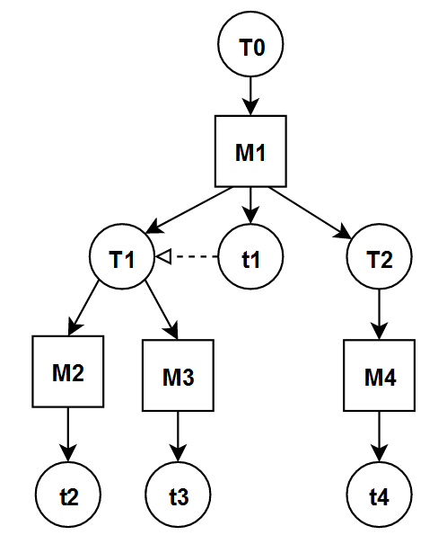
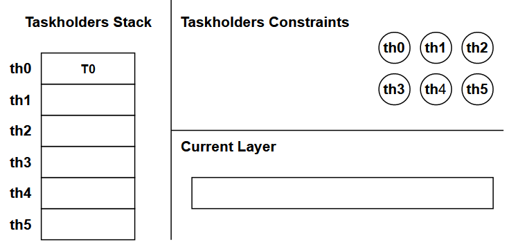
To fix ideas, let us consider the planning problem defined as a task decomposition graph (see Figure 2), a graphical representation of the initial structures of this problem, i.e., taskholders and current layer, is given Figure 6.

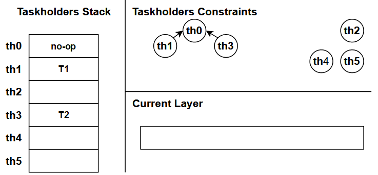
The dynamics of the CPFD procedure (Alg . 1) is defined by three types of STRIPS actions: (1) the first type of actions resolves an unconstrained compound task and update the current task network according to a method decomposition (2) the second type of actions resolves a primitive task and add an action to the current layer; and (3) the last type of actions is the one switching layer, making the algorithm build the next layer of the solution plan. The planning process will choose one action among the three types. Applying one of this action is equivalent to one recursive call of CPFD procedure. The planning process ends when there is no tasks left in the task network, i.e., when all taskholders are empty. These actions are defined as follows:

1. 1.

   Actions for resolving compound tasks: These actions reflect the decomposition of a compound task into subtasks according to a method. It corresponds to the lines 27 to 30 of CPFD procedure. In order to apply these actions, the following must be verified:

   • •

     The taskholder containing the decomposed task is unconstrained.

   • •

     There is enough taskholders remaining in the stack.

   It works on our example as represented Figure 3. The substasks of the method $M_{1}$ decomposing $T_{0}$ are added to the stack of taskholders and the task $T_{0}$ is replaced by the last task of the current task network. As $M_{1}$ as no last task, the no-op action is used. Finally, the ordering constraints are set over the taskholders.

2. 2.

   Actions for resolving primitive tasks: These actions resolve an unconstrained primitive task of the task network and add the resolver action $a\in A$ into the current layer (lines 21 to 23 of Alg. 1). In CPFD procedure, it translates to adding the action resolving a primitive task contained in an unconstrained taskholder to the current layer, removing the primitive task from the taskholder and marking the taskholder as resolved. These actions can be executed when the following conditions are verified:

   • •

     The preconditions of the action are satisfied.

   • •

     The taskholder containing the task is unconstrained.

   • •

     All actions already planned at the plan step are independent with the task.

   An example of application is displayed on Figure 4. The taskholder $th2$ is unconstrained and contains a primitive task $t1$ that can be resolved by the action $a(t1)$. The task is resolved by adding $a(t1)$ to the current layer, $th2$ is emptied and marked as resolved.

   As in Alg. 1, the constraints implied by the resolved taskholder are not removed yet, they will when going to the next layer.

3. 3.

   Action for switching of plan layer: This CTHD action corresponds to switching to the next layer. This action empty the current layer, setting up the next one in the solution plan. It also removes the constraint implying the resolved taskholders. This action can be applied in any situation and works as displayed on Figure  5. In this example, only $th2$ is marked as resolved. After the application of the action, the constraints implying $th2$ are removed, so the constraint between $th2$ and $th1$ is deleted, additionally $th2$ is unmarked as resolved and set as empty. Then the current layer is emptied by removing all actions in it.

In this section we present the STRIPS formulation of the translated problem. Similarly to HTN2STRIPS, our translation depends on an integer parameter denoted $b$ representing the number of taskholders (i.e. the maximum number of tasks in the task network). We first define the predicates used to encode the problem, then we define the encoding of the three types of actions presented above. We end by presenting the initial state and goal state of the translated problem.

Let $P=(L,{\cal T},A,M,I,tn)$ be a HTN problem and let $b\in\mathbb{N}$ the number of taskholders. CTHD encoding generates a STRIPS problem $CPFD(P,b)=(L\cup L^{\prime},A^{\prime},I\cup I^{\prime},G^{\prime})$.

The encoding generates the set propositions $L^{\prime}$ based on the following predicates:

• •

  $(not\_constraint\ ?th1\ ?th2-taskholder)$ represents the fluent constraints over the taskholders. The predicate is inverted for convenience, so when the proposition $(not\_constraint\ th1\ th2)$ is false, it means that the task contained in $th1$ must be planned before the task contained in $th2$.

• •

  $(empty\ ?th-taskholder)$ represents the fact that a taskholder is empty. The proposition $(empty\ th)$ is true if the taskholder $th$ does not contain a task.

• •

  $(in\ ?t-\ task\ ?th\ -\ taskholder)$ is the predicate representing whether or not the task $?t\in{\cal{T}}$ is set in the parameter taskholder. The proposition $(in\ t\ th)$ is true if $t$ is set in $th$.

• •

  $(not\_planned\ ?a-action)$ is true if $a$ is not planned in the current plan step.

• •

  $(prec\_th\ ?th1\ ?th2-taskholder)$ is a predicate defining the static relationship between the taskholders and defines the taskholders stack. So the proposition $(prec\_th\ th1\ th2)$ is true is $th1$ is above $th2$ in the stack. In the following, this order will be fixed and $\forall 0\leq i,j<b$ the proposition $(prec\_th\ th_{i}\ th_{j})$ will be true if and only if $i\leq j$.

• •

  $(resolved\ ?th\ -\ taskholder)$ is a predicate representing either or not a taskholder have been resolved. So the proposition $(resolved\ th)$ is true if the taskholder $th$ have been resolved.
  

The encoding generates the set of actions $A^{\prime}=A_{c}\cup A_{p}\cup A_{l}$ where $A_{c}$ is the set of actions for resolving compound tasks, $A_{p}$ the set of actions for resolving primitive tasks and $A_{l}$ the set of actions for switching of plan layer:

• •

  Actions for resolving compound tasks:
  Let $m=(task(m),pre(m),tn(m))$ and $(task_{1},$ $task_{2},\ldots,task_{k})$ the subtasks in $tn$. We assume that $task_{k}$ is the last task of $tn$. For all methods $m\in M$ there is an action $a_{m}\in A_{c}$ with $k$ parameters $(?th_{1},?th_{2},\ldots,?th_{k})$ defined as follows:

  • –

    $pre(a_{m})=(in\ task(m)\ ?th_{1})\wedge\\ \bigwedge_{i=0}^{b-1}(not\_constraint\ th_{i}\ ?th_{1})\wedge\\ \bigwedge_{i=2}^{k}(prec\_th\ ?th_{i}\ ?th_{i+1})\wedge\\ \bigwedge_{i=2}^{k}(empty\ ?th_{i})$

  • –

    $add(a_{m})=\bigwedge_{i=2}^{k}(in\ task_{i}\ ?th_{i})\wedge(in\ task_{k}\ ?th_{1})$

  • –

    $del(a_{m})=\bigwedge_{i=2}^{k}(empty\ ?th_{i})\wedge\\ \bigwedge_{task_{i}\prec task_{j}}(not\_constraint\ ?th_{i}\ ?th_{j})\wedge\\ \bigwedge_{i=2}^{k}(not\_constraint\ ?th_{i}\ ?th_{0})$

  Note that the $k-1$ last taskholder parameters are required to be ordered according to the static relationship defined by the $prec\_th$ predicate. For instance, if three new taskholders are required to decompose the task in $th6$, $(th6\ th2\ th4\ th7)$ is a valid combination of parameters, while $(th6\ th2\ th5\ th3)$ is not.

• •

  Actions for resolving primitive tasks:
  For all actions $a\in A$ there is an action $a_{p}\in A_{p}$ with one parameter: a taskholder containing $p$ and denoted $?th$. The action is defined as follows:

  • –

    $pre(a_{p})=pre(a)\wedge(in\ task(a)\ ?th)\wedge\\ \bigwedge_{i=0}^{b-1}(not\_constraint\ th_{i}\ ?th)\wedge\\ \bigcup_{t\in nInd(p)}(not\_planned\ ?a)$

  • –

    $add(a_{p})=add(a)\wedge(empty\ ?th)\wedge(resolved\ ?th)$

  • –

    $del(a_{p})=del(a)\wedge(not\_planned\ ?a)$

• •

  Action for switching layer:
  $A_{l}$ is composed of one conditional action $a_{l}$ with no parameter. This action has a non conditional part: emptying the current layer, and a conditional part: unconstraining and making available for a new use the resolved taskholders. It is defined as follows:

  • –

    $pre(a_{l})=\emptyset$

  • –

    $add(a_{l})=\bigwedge_{a\in A}(not\_planned\ ?a)\wedge\\ \forall(?th\ -\ taskholder)$ when $(resolved\ ?th),\\ \bigwedge_{i=0}^{b-1}(not\_constraint\ ?th\ \ th_{i})$

  • –

    $del(a_{l})=\emptyset$

Finally, let us define the encoding for the initial state and goal of the translated problem. The initial state is defined by setting the initial task into the first taskholder. The remaining taskholders are set as empty and ordered in a stack. As there is no constraint over the taskholder yet, all constraints predicate are initialized accordingly.

$I^{\prime}=(in\ task_{0}\ th_{0})\wedge\bigwedge_{1\leq i<b}(empty\ th_{i})\\ \wedge\bigwedge_{1\leq i<j<b}(prec\_th\ th_{i}\ th_{j})\wedge\\ \bigwedge_{0\leq i,j<b}(not\_constraint\ th_{i}\ th_{j})\wedge\\ \bigwedge_{a\in A}(not\_planned\ a)$

The problem is solved when all taskholders are empty, meaning that all task are planned. The goal state is defined accordingly.

$G^{\prime}=\bigwedge_{i=0}^{p-1}(empty\ th_{i})$

If both CTHD and HTN2STRIPS encode HTN solving with taskholders, they aim at finding different kinds of solution plans. While CTHD aims at finding concurrent plans, HTN2STRIPS can only produce sequential ones. In the following, we will experimentally compare the two encodings but one has to keep in mind that CTHD produces plans with higher expressivity than the one produced by HTN2STRIPS.

In addition, while HTN2STRIPS taskholders are unordered, CTHD orders the taskholders into a static stack and imposes an order in which the taskholders parameters are used. The purpose of the stack is to reduce the number of valid operators in the translated problem: let us consider an example with four taskholders and a task $T_{1}$ set in the first taskholder $th1$. $T_{1}$ can be decomposed by a method $m$ into four subtasks $t_{1}$, $t_{2}$, $t_{3}$ and $t_{4}$. The HTN2STRIPS translation, translates this method into $3!$ (equivalent) actions (one for each permutation of the three newly used taskholders). Meanwhile CTHD, by constraining the taskholder a fixed order, translates this method into a single action which corresponds to the HTN2STRIPS action where all taskholders are ordered. In the general case, if $b$ is the progression bound, the number of translated actions generated from a method requiring $k$ new taskholders is equal to the number of permutations of $k$ elements among $b$ for HTN2STRIPS. While the number of generated actions is equal to the number of crescent permutations for CTHD, which is much lower.

References

- Alford et al. (2016) Alford, R.; Behnke, G.; Höller, D.; Bercher, P.; Biundo, S.; and Aha, D. W. 2016. Bound to Plan: Exploiting Classical Heuristics via Automatic Translations of Tail-Recursive HTN Problems. ICAPS’16, 20–28. ISBN 1577357574.
- Alford, Kuter, and Nau (2009) Alford, R.; Kuter, U.; and Nau, D. 2009. Translating HTNs to PDDL: A Small Amount of Domain Knowledge Can Go a Long Way. IJCAI’09, 1629–1634.
- Behnke et al. (2022) Behnke, G.; Pollitt, F.; Höller, D.; Bercher, P.; and Alford, R. 2022. Making Translations to Classical Planning Competitive With Other HTN Planners. In Proceedings of the 36th AAAI Conference on Artificial Intelligence (AAAI 2022). AAAI Press.
- Bercher, Alford, and Höller (2019) Bercher, P.; Alford, R.; and Höller, D. 2019. A Survey on Hierarchical Planning - One Abstract Idea, Many Concrete Realizations. IJCAI 2019, 6267–6275.
- Bercher, Keen, and Biundo (2014) Bercher, P.; Keen, S.; and Biundo, S. 2014. Hybrid Planning Heuristics Based on Task Decomposition Graphs. SoCS 2014, 35–43.
- Bryce and Kambhampati (2007) Bryce, D.; and Kambhampati, S. 2007. A Tutorial on Planning Graph Based Reachability Heuristics. AI Magazine, 28: 47–83.
- Erol (1996) Erol, K. 1996. Hierarchical task network planning: formalization, analysis, and implementation. In Computer Science Departement, University of Maryland, PhD. Thesis.
- Erol, Hendler, and Nau (2003) Erol, K.; Hendler, J.; and Nau, D. 2003. Complexity Results for HTN Planning. Annals of Mathematics and Artificial Intelligence, 18: 69–93.
- Fikes and Nilsson (1971) Fikes, R. E.; and Nilsson, N. J. 1971. STRIPS: A new approach to the application of theorem proving to problem solving. Artificial Intelligence, 2(3): 189–208.
- Georgievski (2020) Georgievski, I. 2020. HTN Planning Domain for Deployment of Cloud Applications. IPC’10, 34–36.
- Ghallab, Nau, and Traverso (2004) Ghallab, M.; Nau, D.; and Traverso, P. 2004. Automated Planning: Theory and Practice.
- Helmert (2011) Helmert, M. 2011. The Fast Downward Planning System. CoRR, abs/1109.6051.
- Hoffmann (2000) Hoffmann, J. 2000. A Heuristic for Domain Independent Planning and Its Use in an Enforced Hill-Climbing Algorithm. In ISMIS 2000, volume 1932, 216–227.
- Hoffmann and Nebel (2011) Hoffmann, J.; and Nebel, B. 2011. The FF Planning System: Fast Plan Generation Through Heuristic Search. 14: 253–302.
- Katz et al. (2018) Katz, M.; Sohrabi, S.; Samulowitz, H.; and Sievers, S. 2018. Delfi: Online planner selection for cost-optimal planning. In Ninth International Planning Competition (IPC-9), 55–62.
- Menif, Jacopin, and Cazenave (2014) Menif, A.; Jacopin, E.; and Cazenave, T. 2014. SHPE: HTN Planning for Video Games. In Third Workshop on Computer Games, CGW 2014, 119–132. Prague, Czech Republic.
- Milot et al. (2021) Milot, A.; Chauveau, E.; Lacroix, S.; and Lesire, C. 2021. Solving Hierarchical Auctions with HTN Planning. In 4th ICAPS workshop on Hierarchical Planning (HPlan). Guangzhou, China.
- Nau et al. (2003) Nau, D.; Au, T.-C.; Ilghami, O.; Kuter, U.; Murdock, J. W.; Wu, D.; and Yaman, F. 2003. SHOP2: An HTN planning system. JAIR, 20: 379–404.
- Pednault (1994) Pednault, E. 1994. ADL and the State-Transition Model of Action. Journal of Logic and Computation, 4(5): 467–512.
- Schreiber et al. (2019) Schreiber, D.; Pellier, D.; Fiorino, H.; and Balyo, T. 2019. Efficient SAT Encodings for Hierarchical Planning. ICAART 2019, 531–538. Prague, Czech Republic.
- Vidal and Geffner (2006) Vidal, V.; and Geffner, H. 2006. Branching and pruning: An optimal temporal POCL planner based on constraint programming. Artificial Intelligence, 170(3): 298–335.