Highly Efficient Structural Learning of Sparse Staged Trees
Abstract
Several structural learning algorithms for staged tree models, an asymmetric extension of Bayesian networks, have been defined. However, they do not scale efficiently as the number of variables considered increases. Here we introduce the first scalable structural learning algorithm for staged trees, which searches over a space of models where only a small number of dependencies can be imposed. A simulation study as well as a real-world application illustrate our routines and the practical use of such data-learned staged trees.
Keywords: Asymmetric conditional independence; Bayesian networks; Probabilistic graphical models; Staged trees; Structural learning.
1 Introduction
Probabilistic graphical models, and in particular Bayesian networks (BNs), are nowadays widely used in machine learning to conveniently represent the relationships existing between the components of a random vector. The directed acyclic graph (DAG) associated to a BN represents graphically (symmetric) conditional independence statements, which can be assessed using the d-separation criterion (Pearl 1988). Although the underlying DAG can be expert-elicited, this is often learned from data using algorithms that explore the space of all possible DAGs (Scutari et al. 2019, see e.g.).
For quite some time it has been noticed that the strict assumption of symmetric conditional independence may be too restrictive to fully represent the relationship between variables in a dataset (Boutilier et al. 1996; Chickering et al. 1997; Friedman and Goldszmidt 1996). However, the development and use in practice of probabilistic graphical models embedding asymmetric conditional independence has been limited (see Hyttinen et al. 2018; Nicolussi and Cazzaro 2021; Talvitie et al. 2019, for some recent proposals). Possible reasons behind the limited use of such models could be: (i) the lack of widely available software; (ii) the complexity of the learning routines; and (iii) the less intuitive visualization of the associated independences which are not explicitly represented by a single graph.
Staged trees (Collazo et al. 2018; Smith and Anderson 2008) are probabilistic graphical models which, starting from an event tree, represent any type of asymmetric conditional independence by a partitioning/coloring of the vertices of the tree. All the model information and the conditional independences can be read directly from the tree and, in particular, from the coloring of the vertices. The stagedtrees R package (Carli et al. 2022) provides a user-friendly implementation of a wide array of structural learning and inferential routines to fit staged trees to data. Therefore, two of the main limitations to the use of asymmetric probabilistic graphical models do not apply to staged trees. Furthermore, a wide toolkit of procedures to work with staged trees have been developed, including handling missing data, sensitivity analysis and exploration of equivalence classes, among others (see Collazo et al. 2018, for details).
On the other hand, learning staged trees from data is complex. Although efficient structural learning algorithms for such models have been implemented (Freeman and Smith 2011; Leonelli and Varando 2021; Silander and Leong 2013, e.g.), they can only work with a limited number of variables. The main reason behind this is the explosion of the size of the model search space as the number of variables considered increases. As an illustration, the number of DAGs over 6 binary variables is 3781503, whilst there are staged trees under the same conditions (Duarte and Solus 2021). Furthermore, the number of DAGs remains constant if variables have more than two levels, whilst the number of staged trees would further increase dramatically.
Recent proposals for efficient structural learning of staged trees look at sub-classes of staged trees, with the aim of reducing the size of the model space. Carli et al. 2020 defined naive staged trees which have the same complexity of a naive BN over the same variables. Leonelli and Varando 2022 considered simple staged trees which have a constrained type of partitioning of the vertices. Duarte and Solus 2021 defined CStrees which only embed symmetric and context-specific types of independence, and not others (Pensar et al. 2016).
One of the first solutions to make structural learning of BNs scalable was to limit the number of parents each variable can have (Friedman et al. 1999; Tsamardinos et al. 2006). This was imposed not only to restrict the model space of possible DAGs, but it also made sense from an applied point of view since most often only a limited number of variables can be expected to have a direct influence on another. The option of setting a maximum number of parents is also available in the standard bnlearn software (Scutari 2010).
Here, we define a sub-class of staged trees embedding the same idea of limiting the number of variables that can have a direct influence to another. As we formalize below, this means that the BN representation associated to such a staged tree is sparse, meaning that it has a small number of edges. A structural learning algorithm for this class of staged trees is introduced and its features are explored in an extensive simulation study.
2 Bayesian Networks and Staged Trees
Before introducing staged trees, we give a formal definition of BNs. We then describe their relationships with staged tree models.
2.1 Bayesian Networks
Let be a DAG with vertex set and edge set . Let be categorical random variables with joint mass function and sample space . For , we let and where . We say that is Markov to if, for ,
where is the parent set of in and is a shorthand for . It is customary to label the vertices of a BN so to respect the topological order of and we henceforth assume that is a topological order of .
The ordered Markov condition implies conditional independences of the form
Henceforth, is assumed to be strictly positive. Let be a DAG and Markov to . The Bayesian network model (associated to ) is
where is the ()-dimensional open probability simplex.
2.2 Staged Trees
Differently to BNs, whose graphical representation is a DAG, staged trees visualize conditional independence by means of a colored tree. Let be a directed, finite, rooted tree with vertex set , root node and edge set . For each , let be the set of edges emanating from and be a set of labels.
An -compatible staged tree is a triple , where is a rooted directed tree and:
- 1.
;
- 2.
For all , if and only if and , or and for some ;
- 3.
is a labelling of the edges such that for some function . The function is called the colouring of the staged tree .
If then and are said to be in the same stage. Therefore, the equivalence classes induced by form a partition of the internal vertices of the tree in stages.
Points 1 and 2 above construct a rooted tree where each root-to-leaf path, or equivalently each leaf, is associated to an element of the sample space . Then a labeling of the edges of such a tree is defined where labels are pairs with one element from a set and the other from the sample space of the corresponding variable in the tree. By construction, -compatible staged trees are such that two vertices can be in the same stage if and only if they correspond to the same sample space.
Figure 1 reports an -compatible staged tree over four binary variables. The coloring given by the function is shown in the vertices and each edge is labeled with . The edge labeling can be read from the graph combining the text label and the color of the emanating vertex. The staging of the staged tree in Figure 1 is given by the partition , , , , , , , and .
The parameter space associated to an -compatible staged tree with labeling is defined as
| (1) |
Equation (1) defines a class of probability mass functions over the edges emanating from any internal vertex coinciding with conditional distributions , and . In the staged tree in Figure 1 the staging implies that the conditional distribution of given and , represented by the edges emanating from , is equal to the conditional distribution of given and . A similar interpretation holds for the staging . This in turn implies that , thus illustrating that the staging of a tree is associated to conditional independence statements.
Let denote the leaves of a staged tree . Given a vertex , there is a unique path in from the root to , denoted as . The depth of a vertex equals the number of edges in . For any path in , let denote the set of edges in the path .
The staged tree model associated to the -compatible staged tree is the image of the map
| (2) |
Therefore, staged trees models are such that atomic probabilities are equal to the product of the edge labels in root-to-leaf paths and coincide with the usual factorization of mass functions via recursive conditioning.
2.3 Staged Trees and Bayesian Networks
Although the relationship between BNs and staged trees was already formalized by Smith and Anderson 2008, a formal procedure to represent a BN as a staged tree has been only recently introduced in Duarte and Solus 2020 and Varando et al. 2021.
Assume is topologically ordered with respect to a DAG and consider an -compatible staged tree with vertex set , edge set and labeling defined via the coloring of the vertices. The staged tree , with vertex set , edge set and labeling so constructed, is called the staged tree model of . Importantly, , i.e. the two models are exactly the same, since they entail exactly the same factorization of the joint probability. Clearly, the staging of represents the Markov conditions associated to the graph .
Varando et al. 2021 approached the reverse problem of transforming a staged tree into a BN. Of course, since staged trees represent more general asymmetric conditional independences, given a staged tree most often there is no BN with DAG such that . However, Varando et al. 2021 introduced an algorithm that, given an -compatible staged tree , finds the minimal DAG such that . Minimal means that such a DAG embeds all symmetric conditional independences that are in and that there are no DAGs with less edges than embedding the same conditional independences.
As an illustration, the staged tree in Figure 1 can be constructed as the from the BN with DAG in Figure 2, embedding the conditional independences and . Conversely, consider the staged tree in Figure 3, which differs from the one in Figure 1 only on a different coloring of the vertices and . Such a staged tree does not embed any symmetric conditional independence, only non-symmetric ones, and therefore there is no DAG such that . Furthermore, the minimal DAG such that is the complete one since the staging of the tree implies direct dependence between every pair of variables.
2.4 Structural Learning Algorithms Inducing Sparsity
Since the model search space of staged trees is huge, we consider here structural learning for a subclass of staged trees that we define next.
Definition 1
A staged tree is in the class of -parents staged trees if the maximum in-degree in is less or equal to .
For instance, the staged tree in Figure 1 is in the class of 2-parents staged trees, whilst the one in Figure 3 is not, since its associated minimal DAG is such that has three parents.
Of course, the class of -parents staged trees is much smaller than the one of -compatible ones, for small values of , and therefore structural learning is expected to be quicker. Here we define a structural learning algorithm to learn a staged tree in the class of -parents staged trees which consists of the following steps: (i) learn a BN with DAG having at most parents (for instance using bnlearn); (ii) construct the equivalent staged tree ; (iii) run the backward hill-climbing algorithm of Carli et al. 2022 which only joins stages together (no splitting of stages) based on the minimization of the model BIC (Görgen et al. 2022). Call the resulting staged tree . It can be easily proven that has at most parents and .
Although the idea of using the staged tree equivalent to a BN as starting point of a structural learning algorithm (or at least using a partial ordering associated to such a BN) is not new (Barclay et al. 2013, see e.g.), here we specifically use such a strategy to limit the complexity of the learned staged tree. This has two major advantages: (i) the speed of the algorithms increases greatly; (ii) the non-symmetric conditional independences can be easily visualized even when a large number of variables are present, as illustrated in Section 4.
3 Experiments
We perform simulation experiments to evaluate the proposed learning strategy for -parents staged trees. Moreover we it compare to standard learning of staged trees and DAGs.
In all the simulated experiments we generated data from random -parents staged trees, which are obtained as follow: (1) A random DAG with fixed topological order is obtained by randomly selecting up to parents uniformly from for each ; (2) The equivalent staged tree is obtained; (3) Stages in are randomly merged with probability . The obtained staged tree is such that is a sub-graph of and thus it is a -parents staged tree; (4) Lastly, we assign random probabilities (uniformly from the simplex) to each stage of the staged tree . Once we generate the random -parents staged tree , we can easily sample observations of from it via sequential sampling (as implemented in the stagedtrees package). For each fixed parameters (, and number of observation sampled) we repeat the experiments times and report averages and standard errors.
3.1 Oracle DAG
We first consider an ideal scenario where we evaluate the performance of the proposed method when the starting DAG is the graph used to generate the true staged tree . We thus run a standard backward hill-climbing (BHC) procedure, as implemented in the stagedtrees package, starting from both the full saturated tree model and starting from the model . All heuristic searches optimize the BIC score.
We plot in Figure 4 the average computation time as a function of the system size and varying the number of maximum parents . For each one of the two approaches we split the computation time in: build time, the time spent building the starting tree; and search time, the time spent running the search algorithm. We can observe that starting the search from the DAG-equivalent tree allows us to scale the algorithm easily up to variables, while the standard approach starting from the full tree become quickly infeasible after variables.
As a sanity check we also compute the normalized hamming distance (the sum across the depth of the tree of the average number of nodes for which coloring needs to change to obtain the same staged tree) and the context intervention distance (Leonelli and Varando 2021) between the true and learned models. As expected the -parents trees obtain better results, which we do not report here for lack of space.
3.2 Learned DAG
We perform now a simulation study similar to the oracle setting but, as in a more realistic scenario, we do not assume knowledge of the DAG . We thus, first estimate a DAG from data using the hill-climbing approach in the bnlearn package (Scutari 2010), and then we apply the BHC learning algorithm starting from the staged tree (bhcdag). We compare the obtained tree to (the tree equivalent to the learned DAG, dag) and the output of the BHC algorithm starting from the full saturated model (bhc). We run replications of the experiment for different system sizes (), for different number of maximum parents in the true DAG () and with sample sizes ranging from to .
In Figure 5 we plot the average (across repetitions) normalized hamming distance between the estimated tree and the true one. We can observe that the -parents staged trees, obtained by the BHC algorithm starting from (bhcdag), are closer to the true data-generating models, with respect to both the output of BHC starting from the saturated model and the tree obtained from the estimated DAG.
4 COVID-19 Drivers and Country Risks
We next extend the analysis of Qazi and Simsekler 2022 who developed a BN to investigate how various country risks and risks associated to the COVID-19 epidemics relate to each other. In particular here we focus on how various types of risks affect the overall country risk associated to COVID-19.
For this purpose, as in Qazi and Simsekler 2022, the dataset used in the analysis comes from the combination of two sources. Country-level exposure to COVID-19 risks are retrieved from INFORM (INFORM 2022). The data comprises of a score between zero and ten for 191 countries for three drivers of COVID-19 risks, namely hazard and exposure, vulnerability, and lack of coping capacity. An overall COVID-19 risk index, again between zero and ten, is constructed from these three drivers. Country-level exposure to various socioeconomic risk factors are collected from Euler Hermes (Euler Hermes 2022). The ratings for five drivers of country risk, namely economic, political, financing, commercial and business environment are collected for 188 countries (the indexes are integer-valued between one and four or six). The combined dataset comprises 181 countries. Each variable is discretized into two levels using the clustering method from the arules package (Hahsler et al. 2005).
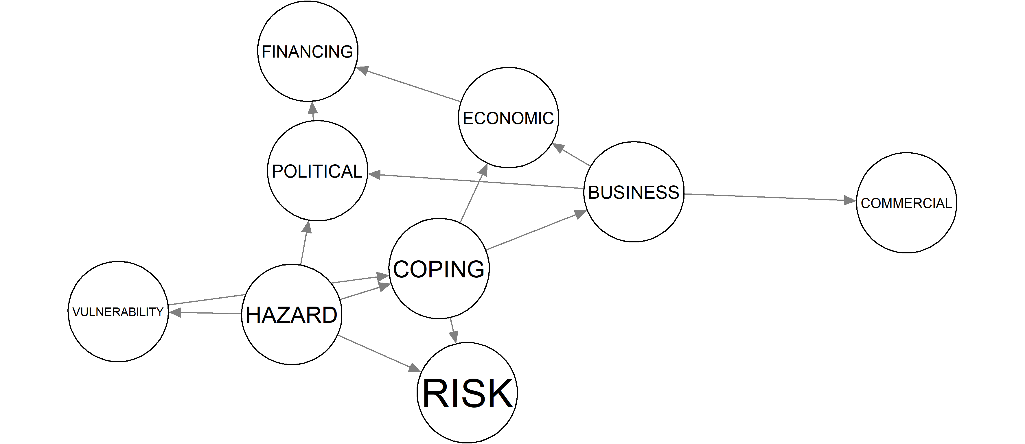
A BN is learned using the hc function of the bnlearn package with the constraint that the overall COVID-19 risk must be a leaf of the network and is reported in Figure 6. Without specifying it, the learned BN is such that each vertex has at most two parents. The DAG suggests that COVID-19 risk is conditionally independent of all other drivers given the lack of coping capacity and hazard & exposure.
Starting from this BN, a staged tree in the class of 2-parents staged trees is learned using the algorithm of Section 2.4. This staged tree provides a better representation of the data since it has a BIC of 1521.965, compared to the BIC of 1547.634 of the BN. The learned staged tree embeds the same set of symmetric conditional independences as in the BN of Figure 2, but also non-symmetric ones. Of course, the full tree cannot be easily visualized since, for instance, there are vertices with depth nine. However, since it is known that COVID-19 risk only depends on the lack of coping capacity and hazard & exposure we can construct the staged tree over these three variables only and easily visualize further non-symmetric dependences. This is reported in Figure 7, which shows the presence of the context-specific independence between COVID-19 risk and hazard & exposure for lack of coping capacity equal to low. Similar interpretations could be drawn by constructing the “partial” staged trees associated to other variables.
Of course a generic staged tree would provide a better representation of the data. For instance, one learned with the backward hill-climbing of Carli et al. 2022 starting from the saturated model has a BIC of 1453.587. However, its complete visualization is again unfeasible and plots as the one of Figure 7 are in general not viable since there are no constraints on the number of parents of . Indeed, whilst the DAG for the tree in Figure 7 has 13 edges (as the DAG in Figure 6), the DAG from the generic staged tree is complete and consisting of 36 edges, meaning that all variables are directly related to one another.
5 Discussion
We defined a novel sub-class of staged tree models borrowing the idea of limiting the number of parents in BNs. A structural learning algorithm for such a class has been introduced and its properties illustrated both in simulation experiments and in a real-world application.
The number of parents of a variable in the staged tree is limited by those of the learned BN. For instance, in our application, although no limit on the number of parents was set, there were at most two parents. However, non-symmetric dependences may have been missed by the BN learning algorithm which is specifically designed to account for symmetric ones. One possibility could be to add edges to the learned BN, for instance between variables such that their conditional mutual information is large, and then run a backward hill-climbing algorithm of Carli et al. 2022 over that BN. The feasibility of such an algorithm is the focus of current research.
Acknowledgements
Gherardo Varando’s work was funded by the European Research Council (ERC) Synergy Grant “Understanding and Modelling the Earth System with Machine Learning (USMILE)” under Grant Agreement No 855187.
References
- Barclay et al. (2013) L. M. Barclay, J. L. Hutton, and J. Q. Smith. Refining a Bayesian network using a chain event graph. International Journal of Approximate Reasoning, 54:1300–1309, 2013.
- Boutilier et al. (1996) C. Boutilier, N. Friedman, M. Goldszmidt, and D. Koller. Context-specific independence in Bayesian networks. In Proceedings of the Twelfth Conference on Uncertainty in Artificial Intelligence, pages 115–123, 1996.
- Carli et al. (2020) F. Carli, M. Leonelli, and G. Varando. A new class of generative classifiers based on staged tree models. arXiv:2012.13798, 2020.
- Carli et al. (2022) F. Carli, M. Leonelli, E. Riccomagno, and G. Varando. The R package stagedtrees for structural learning of stratified staged trees. Journal of Statistical Software, 102(6):1–30, 2022.
- Chickering et al. (1997) D. M. Chickering, D. Heckerman, and C. Meek. A Bayesian approach to learning Bayesian networks with local structure. In Proceedings of 13th Conference on Uncertainty in Artificial Intelligence, pages 80–89, 1997.
- Collazo et al. (2018) R. Collazo, C. Görgen, and J. Smith. Chain event graphs. Chapmann & Hall, 2018.
- Duarte and Solus (2020) E. Duarte and L. Solus. Algebraic geometry of discrete interventional models. arXiv:2012.03593, 2020.
- Duarte and Solus (2021) E. Duarte and L. Solus. Representation of context-specific causal models with observational and interventional data. arXiv:2101.09271, 2021.
- Euler Hermes (2022) Euler Hermes. Country risk reports. Retrieved from: https://www.eulerherm es.com/en_global/economic-research/country-reports.html, 2022.
- Freeman and Smith (2011) G. Freeman and J. Q. Smith. Bayesian MAP model selection of chain event graphs. Journal of Multivariate Analysis, 102(7):1152–1165, 2011.
- Friedman and Goldszmidt (1996) N. Friedman and M. Goldszmidt. Learning Bayesian networks with local structure. In Proceedings of the 12th Conference on Uncertainty in Artificial Intelligence, pages 252–262, 1996.
- Friedman et al. (1999) N. Friedman, I. Nachman, and D. Pe’er. Learning Bayesian network structure from massive datasets: The “sparse candidate” algorithm. In Proceedings of the 15th Conference on Uncertainty in Artificial Intelligence, pages 206–215, 1999.
- Görgen et al. (2022) C. Görgen, M. Leonelli, and O. Marigliano. The curved exponential family of a staged tree. Electronic Journal of Statistics, 16(1):2607–2620, 2022.
- Hahsler et al. (2005) M. Hahsler, B. Gruen, and K. Hornik. arules – A computational environment for mining association rules and frequent item sets. Journal of Statistical Software, 14(15):1–25, 2005.
- Hyttinen et al. (2018) A. Hyttinen, J. Pensar, J. Kontinen, and J. Corander. Structure learning for Bayesian networks over labeled DAGs. In International Conference on Probabilistic Graphical Models, pages 133–144, 2018.
- INFORM (2022) INFORM. COVID-19 risk index. Retrieved from: https://drmkc.jrc. ec.europa.eu/inform-index/INFORM-Covid-19, 2022.
- Leonelli and Varando (2021) M. Leonelli and G. Varando. Context-specific causal discovery for categorical data using staged trees. arXiv:2106.04416, 2021.
- Leonelli and Varando (2022) M. Leonelli and G. Varando. Structural learning of simple staged trees. arXiv:2203.04390, 2022.
- Nicolussi and Cazzaro (2021) F. Nicolussi and M. Cazzaro. Context-specific independencies in stratified chain regression graphical models. Bernoulli, 27(3):2091–2116, 2021.
- Pearl (1988) J. Pearl. Probabilistic reasoning in intelligent systems: networks of plausible inference. Morgan Kaufmann, 1988.
- Pensar et al. (2016) J. Pensar, H. Nyman, J. Lintusaari, and J. Corander. The role of local partial independence in learning of Bayesian networks. International Journal of Approximate Reasoning, 69:91–105, 2016.
- Qazi and Simsekler (2022) A. Qazi and M. C. E. Simsekler. Nexus between drivers of COVID-19 and country risks. Socio-Economic Planning Sciences, page 101276, 2022.
- Scutari (2010) M. Scutari. Learning Bayesian networks with the bnlearn R package. Journal of Statistical Software, 35(3):1–22, 2010.
- Scutari et al. (2019) M. Scutari, C. E. Graafland, and J. M. Gutiérrez. Who learns better Bayesian network structures: Accuracy and speed of structure learning algorithms. International Journal of Approximate Reasoning, 115:235–253, 2019.
- Silander and Leong (2013) T. Silander and T. Leong. A dynamic programming algorithm for learning chain event graphs. In Proceedings of the International Conference on Discovery Science, pages 201–216, 2013.
- Smith and Anderson (2008) J. Smith and P. Anderson. Conditional independence and chain event graphs. Artificial Intelligence, 172(1):42 – 68, 2008.
- Talvitie et al. (2019) T. Talvitie, R. Eggeling, and M. Koivisto. Learning Bayesian networks with local structure, mixed variables, and exact algorithms. International Journal of Approximate Reasoning, 115:69–95, 2019.
- Tsamardinos et al. (2006) I. Tsamardinos, L. E. Brown, and C. F. Aliferis. The max-min hill-climbing Bayesian network structure learning algorithm. Machine Learning, 65(1):31–78, 2006.
- Varando et al. (2021) G. Varando, F. Carli, and M. Leonelli. Staged trees and asymmetry-labeled DAGs. arXiv:2108.01994, 2021.