Probabilistic forecasting of bus travel time with a Bayesian Gaussian mixture modelJournal: Arxiv

Deterministic forecasting model for bus travel time includes time series models and machine learning approaches. Time series model often considers bus travel time as a function of its past observations. Using time series model to forecast travel time, one important step is to construct a standard time series of bus travel time from bus data. Farhan et al. 2002 used HA model to predict the bus travel time. Madzlan et al. 2010 applied ARIMA model to forecast bus route travel time. The forecasting accuracy of time series model highly depend on the characteristics of historical travel time data. If a time series has a stationary pattern or mixture of patterns, time series model can perform well. However, bus travel time is not a standard stationary time series due to the factors like road congestion, dynamic passenger flow, traffic accidents, etc. Therefore, time series model is strictly limited for bus travel time forecasting.

Machine learning approaches have the ability to reveal complex patterns and learn non-linear relationships from data. Existing machine learning models for bus travel time forecasting include ANN, SVM, KF, and the hybrid models. Chien et al. 2002 developed two ANN-based models to forecast bus arrival time under link-based and stop-based route constructions; results show that these two ANN-based models have good performance. Similarly, the studies by Gurmu and Fan 2014, Jeong and Rilett 2004 indicate that ANN-based models outperform HA and regression models for bus travel time forecasting. SVM has been applied as a useful method for forecasting bus travel time. Some studies (Bin et al. 2006; Yu et al. 2011; Yang et al. 2016; Xu and Ying 2017; Ma et al. 2019) have shown SVM outperforms linear regression and time series models. KF is an efficient learning algorithm as it has the ability to update the time-dependent state when new observations become available continuously. Cathey and Dailey 2003 proposed KF model for bus travel time forecasting using real-time and historical data. However, this work did not compared KF model with other developed machine learning models. Some hybrid methods are developed to combine the advantages of these machine learning models. Yu et al. 2018 proposed an approach combining k-nearest neighbors algorithm (KNN) and Random Forest (RF); results shows that the hybrid model outperformed KNN, SVM, RF; however, this method has the problem of low computational efficiency. Zhang et al. 2021 developed a hybrid method to combine SVM with KF, RF and ARIMA respectively; results show that SVM-KF outperforms other hybrid models. Chen et al. 2004 combined ANN and KF algorithm to forecast the arrival time. Based on this research, Bai et al. 2015 replaced ANN with SVM, and results show that SVM-KF performs better than ANN-KF. Kumar et al. 2018 used KNN algorithm to identify significant input variables, and then combining exponential smoothing technique with recursive estimation scheme based on Kalman Filtering method to forecast bus travel time. Recently, Osman et al. 2021 and Alam et al. 2021 used LSTM to forecast bus travel timne; results show that LSTM performs better than ANN, SVR, ARIMA and HA. Similarly, He et al. 2020 applied LSTM for bus travel time prediction but they took consideration into the impact of heterogeneous traffic patterns. Petersen et al. 2019 proposed a deep neural network with the combination of convolutional and LSTM layers for bus travel time prediction.

There are only a few studies on probabilistic forecasting for bus travel time. Dai et al. 2019 proposed a probabilistic model to estimate bus travel time considering the link running time and station dwell time. The authors assumed that: the link travel time is composed of the link running time and the station dwell time, and they are independent; the link running time follows shifted log-normal distribution; the station dwell time is the sum of the queueing time, the passengers loading/unloadding time, and the merging time (the bus merges into the main road traffic). They did not model the correlations between link running times and station dwell times while the correlations are very important for bus travel time forecasting. Ma et al. 2017 proposed a generalized Markov chain approach for estimating the probability distribution of bus trip travel times from link travel time distributions and takes into consideration correlations in time and space. They first used clustering method to cluster link travel time observations, and then using a logit model to develop the transition probability estimation; finally, using a Markov chain procedure, the probability distribution of the trip travel time can be estimated. However, the Markov chain in this framework only models the correlation between adjacent link travel times but ignores the long-range correlation. Huang et al. 2021 proposed two data-driven methods based on the Functional Data Analysis (FDA) and Bayesian Support Vector Regression (BSVR) to forecast the distribution of bus travel time. Both FDA and BSVR are essentially kernel methods. FDA approach is a well-proven mathematical way to describe the stochastic process of link travel time and can provide a continuous-time link travel time forecasting, while BSVR can provide a discrete-time link travel time forecasting with a prescribed discretization interval. The authors utilize the FDA and BSVR for each specific link and then add up relevant link travel times; thus they ignore the link travel time correlation. Büchel and Corman 2022a proposed a hidden Markov chain framework to estimate bus travel time distribution. This framework can capture the dependency structure of consecutive link running times and includes conditional correlations. Moreover, it also captures the dependency of consecutive link dwell times. However, this model only describe the correlations between consecutive link travel times and fails to model long-range correlations. Ricard et al. 2022 proposed two types of probabilistic models: similarity-based density estimation models and a smoothed Logistic Regression for probabilistic classification model. Similarity-based density estimation models first find the set of similar trips and then estimate the density of the particular set by fitting a parametric, semi-parametric or non-parametric model. Multinomial logistic regression is used for probabilistic classification and its generated probability mass function can be smoothed into a probability density function. The authors developed these two methods in order to make a long-term forecast for bus travel time, thus they did not consider to use the feature of link travel time. Büchel and Corman 2022b proposed Bayesian network to forecast bus travel time distribution. They assumed that: the dwell time of a given bus at a given stop depends on the dwell time of the same bus at the previous stop, dwell time of the previous bus at the same stop, and the headway from the previous bus; the running time depends on the running time of the same bus in the previous link and the running time of the previous bus in the same link. This Bayesian framework only consider the dependency between adjacent link travel times but ignore the long-range correlations in bus link travel times.

Although work on probabilistic forecasting for bus travel time is scare, there are some studies on modeling bus travel time distributions, mostly with the objective of quantifying the bus travel time reliability (Büchel and Corman 2020). Bus travel time distribution modeling can provide a foundation for probabilistic forecasting. Taylor 1982 collected bus data and pointed out bus link travel time follows a normal distribution. Mazloumi et al. 2010 explored the travel time distributions for different departure time windows at different times of the day; results show that in narrower departure time windows, bus travel time distributions are best characterized by normal distributions. For wider departure time windows, peak-hour travel times follow normal distributions, while off-peak travel times follow log-normal distributions. Similarly, Rahman et al. 2018 analyzed the bus travel time distributions for different spatial horizon; results show that log-normal distribution is more appropriate for short-term horizon, while normal distribution is more suitable for long-term horizon. Uno et al. 2009 reveled bus link travel time on arterial roadway is positively skewed and generally follows a log-normal distribution. Kieu et al. 2015 also recommended a log-normal distribution as the best fit of bus travel time on urban roads. Büchel and Corman 2018 compared the unimodal distributions including normal, weibull, log-normal, gamma, cauchy, and logistic distribution; results show that the log-normal probability distribution is a good fit for bus travel times at peak and off-peak conditions. Chepuri et al. 2020 compared the Burr, generalized extreme value (GEV), and Log-normal distributions for bus travel time, and results shows that GEV distribution performs the best. Similarly, Harsha and Mulangi 2021 considered seven travel time distributions (including Burr, GEV, Gamma, log-logistic, log-normal, normal and Weibull distributions) and evaluated their performance; results show that GEV distribution performs the best. Ma et al. 2016 compared unimodal distribution and multi-modal distribution for bus link travel time. They found that the normal, log-normal, logistic, log-logistic, and Gamma distributions have a relatively similar performance, and the Gaussian mixture model performs much better in terms of accuracy, robustness, and interpretability.

In summary, existing studies mainly concerned with the deterministic forecasting instead of probabilistic forecasting for bus travel time. Although a few studies have developed probabilistic forecasting for bus travel time, there are some limitations: (1) ignoring the complex link travel time correlation/covariance; (2) ignoring the correlation between buses.

A bus link (or simply a link) is the directional road segment between two adjacent bus stops in a bus route. In this paper, the bus travel time on the $j$-th link is defined as the time difference between the arrival of a bus at the $j$-th and the $(j+1)$-th bus stop, including the bus waiting time at the $j$-th bus stop. Link travel time of buses can be obtained from various types of data sources, such as smart card data, automatic vehicle location (AVL) data, and automatic bus announcing system. Next, we denote $\ell_{i,j}$ to be the link travel time of the $i$-th bus on the $j$-th link. With these definitions, the trip travel time of the $i$-th bus from stop $j_{1}$ to stop $j_{2}$ can be readily calculated by $\sum_{j=j_{1}}^{j_{2}}\ell_{i,j}$.

This paper focuses on forecasting the travel time of a bus on its upcoming links and trips. A previous work (Chen et al. 2022) has shown that link travel time within a single bus trip can be significantly correlated, and using such correlation can improve bus travel time forecasting. A limitation of the previous work is that the dependencies of the travel time among different buses are ignored. Considering the close spatiotemporal distance and similar traffic conditions of two adjacent buses, it is tempting to use the travel time information of a leading bus to forecast the travel time of the next (following) bus. Inspired by this, on top of the previous work, this paper further leverage the travel time correlation between adjacent buses to improve bus travel time forecasting.

The link travel time of bus $i$ on a bus route with $n$ links ($n+1$ bus stops) can be aggregated into a vector $\boldsymbol{\ell}_{i}=\left[\ell_{i,1},\ell_{i,2},\cdots,\ell_{i,n}\right]^{\top}$. We define an augmented random variable $\boldsymbol{x}$ to capture the link travel time correlation between two adjacent buses. The link travel time and the headway of each two adjacent buses (a following bus $i$ and a leading bus $i-1$) produce a sample of $\boldsymbol{x}$:

where the headway $h_{i,j}$ is the time interval between the arrival of the $i$-th bus and the $(i-1)$-th bus at the $j$-th bus stop (we do not count the headway at the last bus stop). Note that there is an inherent relationship between the link travel time and the headway:

Therefore, the $3n$ dimensional random variable $\boldsymbol{x}$ has only $2n+1$ degrees of freedom. The inclusion of headway explicitly bonds $\boldsymbol{\ell}_{i}$ with $\boldsymbol{\ell}_{i-1}$, which efficiently utilizes the link travel time of the leading bus in forecasting the link travel time of the following bus.

Missing and ragged values are unavoidable in real-world link travel time data. Using the relationship between adjacent buses can enhance the accuracy of the missing value imputation. We use the method proposed by Chen et al. 2022 to jointly formulate the missing/ragged values and the headway constraints from Eq. (2). Consider the example in Fig. 1 where the arrival time of bus $i$ at stop $\#3$ cannot be observed. The headway $h_{i,3}$ becomes a missing value. Although individual values of $\ell_{i,2}$, $\ell_{i,3}$ are missing, the sum of the link travel time $\left(\ell_{i,2}+\ell_{i,3}\right)$ can be inferred from the bus arrival time at the upstream and the downstream stops, which is a case of ragged value. Next, the missing/ragged values and headway constraints can be summarized into a linear equation:

where we call $\mathbf{G}_{i}$ the alignment matrix and $\boldsymbol{r}_{i}$ the recording vector for bus $i$. An alignment matrix is a matrix with elements in $\left\{-1,0,1\right\}$ that encodes missing/ragged positions and headway constraints. The recording vector $\boldsymbol{r}_{i}$ records all observed information attached with $\boldsymbol{x}_{i}$. The hyperplane defined by Eq. (3) is the support of random variable $\boldsymbol{x}$.

Alignment matrices and recording vectors can be directly accessed from the source data, but the values of $\boldsymbol{x}_{i}$ are not always available because of the data missing problem. Next, the main task is to estimate the probability distribution (a Gaussian mixture model) of the augmented random variable $\boldsymbol{x}$ using historical alignment matrices $\left\{\mathbf{G}_{i}\right\}$ and recording vectors $\left\{\boldsymbol{r}_{i}\right\}$. After getting the probabilistic distribution of $\boldsymbol{x}$, we can forecast the bus travel time on upcoming links by calculating the conditional probability given the travel time of the leading buses and upstream links. The forecasting procedure is elucidated in Section 3.5.

The distributions of bus link travel times are often positively skewed, heavy-tailed, and sometimes multi-modal. Ma et al. 2016 compared several unimodal distributions (including normal, log-normal, logistic, log-logistic, and Gamma distributions) and multi-modal distributions for bus travel time, and suggested using Gaussian mixture models for bus link travel times. Therefore, we use multivariate Gaussian mixture distributions to model the augmented random variable $\boldsymbol{x}$. Moreover, we divide a day into $T$ periods and assume the mixing coefficients are different for each period to capture the temporal differences. When not considering the headway constraints in Eq. (3), the augmented random variable at the $t$-th period follows a multivariate Gaussian mixture model:

where we use a superscript $(\cdot)^{t}$ to mark the time period; $K$ is the number of components; $\pi_{k}^{t}$ is a mixing coefficient with $\sum_{k=1}^{K}\pi_{k}^{t}=1$ and $\pi_{k}^{t}\geq 0$; the $k$-th component follows a multivariate Gaussian distribution with a mean vector $\boldsymbol{\mu}_{k}\in\mathbb{R}^{3n}$ and a covariance matrix $\boldsymbol{\Sigma}_{k}\in\mathbb{R}^{3n\times 3n}$. When considering the linear constraints in Eq. (3), the distribution of $\boldsymbol{x}_{t}$ is the multivariate Gaussian mixture model in Eq. (4) truncated on the hyperplane defined by Eq. (3).

The augmented link travel time of each period is characterized by a mixture of several shared Gaussian distributions; this structure is essentially similar to the classical topic model (Blei et al. 2003). Fig. 2 shows the overall graphical representation of our Bayesian multivariate Gaussian mixture model that can handle missing, ragged values, and headway constraints. Assume there are $M^{t}$ buses at period $t$, we have $\left\{\boldsymbol{x}_{i}^{t}\right\}_{t=1,i=1}^{T,M^{t}}$ to be a set of “latent” realizations/samples drawn from the multivariate Gaussian mixture distributions truncated on the hyperplanes from Eq. (3). We need to estimate parameters $\left\{\boldsymbol{\pi}^{t}=[\pi_{1}^{t},\pi_{2}^{t},\cdots,\pi_{K}^{t}]^{\top}\right\}_{t=1}^{T}$, $\left\{\boldsymbol{\mu}_{k}\right\}_{k=1}^{K}$, and $\left\{\boldsymbol{\Sigma}_{k}\right\}_{k=1}^{K}$ using the alignment matrices $\mathcal{G}=\left\{{\mathbf{G}}_{i}^{t}\right\}_{t=1,i=1}^{T,M_{t}}$ and the recording vectors $\mathcal{R}=\left\{\boldsymbol{r}_{i}^{t}\right\}_{t=1,i=1}^{T,M_{t}}$. In a Bayesian setting, we use a conjugate Gaussian-inverse-Wishart prior on $\boldsymbol{\mu}_{k}$ and $\boldsymbol{\Sigma}_{k}$ and a Dirichlet prior on $\boldsymbol{\pi}^{t}$ for efficient inference (Gelman et al. 2013). The overall data generation process is summarized as:

where $\boldsymbol{\alpha}$ is the concentration parameter of the Dirichlet distribution; $\mathcal{W}^{-1}\left(\boldsymbol{\Psi}_{0},\nu_{0}\right)$ is the inverse-Wishart distribution with a scale matrix $\boldsymbol{\Psi}_{0}$ and $\nu_{0}$ degrees of freedom; $\boldsymbol{\mu}_{0}$ and $\lambda_{0}$ are parameters for the Gaussian prior.

Based on the graphical model illustrated in Fig. 2, we can derive an efficient MCMC scheme using Gibbs sampling. For simplicity, we let $\mathcal{X}=\left\{\boldsymbol{x}_{i}^{t}\right\}_{t=1,i=1}^{T,M^{t}}$ denote the full set of the “latent” augmented variable for the $\sum_{t=1}^{T}M^{t}$ bus pairs, and let $\Theta=\left\{\boldsymbol{\mu}_{0},\lambda_{0},\boldsymbol{\Psi}_{0},\nu_{0}\right\}$ denote the set of hyperparameters for the Gaussian-inverse-Wishart prior distribution in Eqs. (6) and (7). Moreover, we let $\mathcal{X}_{k}^{t}$ denote the set of data vectors at period $t$ belonging to mixture component $k$ and $\mathcal{X}_{k}$ denote the set of all data vectors belonging to mixture $k$. We start the Gibbs sampling with random initialization for all variables and then iteratively sample each variable from its conditional distribution on other variables:

• 1.

  Sample $\boldsymbol{\pi}_{t}$ from $p\left(\boldsymbol{\pi}^{t}\mid\boldsymbol{z}^{t},\boldsymbol{\alpha}\right)$. The conditional distribution is $p\left(\boldsymbol{\pi}^{t}\mid\boldsymbol{z}^{t},\boldsymbol{\alpha}\right)\propto p\left(\boldsymbol{\pi}^{t}\mid\boldsymbol{\alpha}\right)p\left(\boldsymbol{z}^{t}\mid\boldsymbol{\pi}^{t}\right)$. The prior distribution $p\left(\boldsymbol{\pi}^{t}\mid\boldsymbol{\alpha}\right)=\text{Dirichlet}\left(\boldsymbol{\pi}^{t}\mid\boldsymbol{\alpha}\right)\propto\prod_{k=1}^{K}{\pi_{k}^{t}}^{\alpha_{k}-1}$, and $p\left(\boldsymbol{z}^{t}\mid\boldsymbol{\pi}^{t}\right)$ can be seen as a multinomial distribution $p\left(\boldsymbol{z}^{t}\mid\boldsymbol{\pi}^{t}\right)=\text{Multinomial}_{K}\left(\boldsymbol{z}^{t}\mid N,\boldsymbol{\pi}^{t}\right)\propto\prod_{k=1}^{K}{\pi_{k}^{t}}^{M_{k}^{t}}$, where $M_{k}^{t}$ is the number of $\left\{z_{i}^{t}\right\}_{i=1}^{M^{t}}$ assigned to cluster $k$. Therefore, the conditional posterior distribution is a Dirichlet distribution:

  $$p\left(\boldsymbol{\pi}^{t}\mid\boldsymbol{z}^{t},\boldsymbol{\alpha}\right)\sim\text{Dirichlet}\left(M_{1}^{t}+\alpha_{1},M_{2}^{t}+\alpha_{2},\cdots,M_{K}^{t}+\alpha_{K}\right).$$

  (11)

• 2.

  Sample $z_{i}^{t}$ from $p\left(z_{i}^{t}\mid\boldsymbol{\pi}_{i}^{t},\boldsymbol{\mu},\boldsymbol{\Sigma},\boldsymbol{x}_{i}^{t}\right)$. The conditional distribution of assignment for each observation is given by $p\left(z_{i}^{t}=k\mid\boldsymbol{\pi}_{i}^{t},\boldsymbol{\mu},\boldsymbol{\Sigma},\boldsymbol{x}_{i}^{t}\right)\propto p\left(z_{i}^{t}=k\mid\boldsymbol{\pi}^{t}\right)p\left(\boldsymbol{x}_{i}^{t}\mid\boldsymbol{\mu},\boldsymbol{\Sigma}\right)=\pi_{k}^{t}\mathcal{N}\left(\boldsymbol{x}_{i}^{t}\mid\boldsymbol{\mu}_{k},\boldsymbol{\Sigma}_{k}\right)$. Then we can do the normalization to obtain the conditional discrete distribution over $z_{i}^{t}$ by

  $$p\left({z_{i}^{t}=k}\mid\boldsymbol{\pi}^{t},\boldsymbol{\mu},\boldsymbol{\Sigma},\boldsymbol{x}_{i}^{t}\right)=\frac{\pi_{k}^{t}\mathcal{N}\left(\boldsymbol{x}_{i}^{t}\mid\boldsymbol{\mu}_{k},\boldsymbol{\Sigma}_{k}\right)}{\sum_{m=1}^{K}\pi_{m}^{t}\mathcal{N}\left(\boldsymbol{x}_{i}^{t}\mid\boldsymbol{\mu}_{m},\boldsymbol{\Sigma}_{m}\right)}.$$

  (12)

• 3.

  Sample $(\boldsymbol{\mu}_{k},\boldsymbol{\Sigma}_{k})$ from $p\left(\boldsymbol{\mu},\boldsymbol{\Sigma}\mid\mathcal{X}_{k},\Theta\right)$. Thanks to the conjugate prior distribution, the conditional distribution of the mean vector and the covariance matrix $p\left(\boldsymbol{\mu}_{k},\boldsymbol{\Sigma}_{k}\mid\mathcal{X}_{k},\Theta\right)$ is a Gaussian-inverse-Wishart distribution:

  $$p\left(\boldsymbol{\mu}_{k},\boldsymbol{\Sigma}_{k}\mid\mathcal{X}_{k},\Theta\right)\sim\mathcal{N}\left(\boldsymbol{\mu}_{k}\mid\boldsymbol{\mu}_{0}^{*},\frac{1}{\lambda_{0}^{*}}\boldsymbol{\Sigma}_{k}\right)\mathcal{W}^{-1}\left(\boldsymbol{\Sigma}_{k}\mid\boldsymbol{\Psi}_{0}^{*},\nu_{0}^{*}\right),$$

  (13)

  where

  	$\displaystyle\boldsymbol{\mu}_{0}^{*}=\frac{\lambda_{0}\boldsymbol{\mu}_{0}+M_{k}\bar{\boldsymbol{x}}}{\lambda_{0}+M_{k}},\qquad\lambda_{0}^{*}=\lambda_{0}+M_{k},\qquad\nu_{0}^{*}=\nu_{0}+M_{k},\qquad\bar{\boldsymbol{x}}=\frac{1}{M_{k}}\sum_{t=1}^{T}\sum_{i=1}^{M_{k}^{t}}\boldsymbol{x}_{i}^{t},$		(14)
  	$\displaystyle M_{k}=\sum_{t=1}^{T}M_{k}^{t},\quad\boldsymbol{\Psi}_{0}^{*}=\boldsymbol{\Psi}_{0}+\boldsymbol{\mathrm{S}}+\frac{\lambda_{0}M_{k}}{\lambda_{0}+M_{k}}\left(\bar{\boldsymbol{x}}-\boldsymbol{\mu_{0}}\right)\left(\bar{\boldsymbol{x}}-\boldsymbol{\mu_{0}}\right)^{\top},\quad\boldsymbol{\mathrm{S}}=\sum_{t=1}^{T}\sum_{i=1}^{M_{k}^{t}}\left(\boldsymbol{x}_{i}^{t}-\bar{\boldsymbol{x}}\right)\left(\boldsymbol{x}_{i}^{t}-\bar{\boldsymbol{x}}\right)^{\top}.$

• 4.

  Sample $\mathcal{X}$ from $p\left(\mathcal{X}\mid\boldsymbol{\mu},\boldsymbol{\Sigma},\boldsymbol{z},\mathcal{R},\mathcal{G}\right)$. At this step, we no longer have a simple analytical formulation to sample $\mathcal{X}$ due to the linear constraints in Eq. (10). Here, the conditional distribution can be factorized as

  $$p\left(\mathcal{X}\mid\boldsymbol{\mu},\boldsymbol{\Sigma},\boldsymbol{z},\mathcal{R},\mathcal{G}\right)=\prod_{t=1}^{T}\prod_{i=1}^{M^{t}}{p\left(\boldsymbol{x}_{i}^{t}\mid\boldsymbol{\mu}_{z_{i}^{t}},\boldsymbol{\Sigma}_{z_{i}^{t}},\boldsymbol{r}_{i}^{t},{\mathbf{G}}_{i}^{t}\right)}.$$

  (15)

  Consequently, we can draw sample of the bus-pair vector $\boldsymbol{x}_{i}^{t}$ independently. The conditional distribution of $\boldsymbol{x}_{i}^{t}$ in Eq. (15) can be regarded as a multivariate Gaussian distribution truncated on the intersection with a hyperplane, i.e.,

  $$\boldsymbol{x}_{i}^{t}\,|\,z_{i}^{t}=k\sim\mathcal{N}_{\mathcal{S}_{i}^{t}}\left(\boldsymbol{\mu}_{k},\boldsymbol{\Sigma}_{k}\right),\quad\mathcal{S}_{i}^{t}=\left\{\boldsymbol{x}_{i}^{t}\mid{\mathbf{G}}_{i}^{t}\boldsymbol{x}_{i}^{t}=\boldsymbol{r}_{i}^{t}\right\}.$$

  (16)

  The probability density function of the hyperplane-truncated multivariate Gaussian is

  $$p(\boldsymbol{x}_{i}^{t}\mid\boldsymbol{\mu}_{k},\boldsymbol{\Sigma}_{k},\boldsymbol{r}_{i}^{t},\mathbf{G}_{i}^{t})=\frac{1}{Z_{i}^{t}}\exp\left[-\frac{1}{2}(\boldsymbol{x}_{i}^{t}-\boldsymbol{\mu}_{z_{i}^{t}})^{T}\boldsymbol{\Sigma}_{z_{i}^{t}}^{-1}(\boldsymbol{x}_{i}^{t}-\boldsymbol{\mu}_{z_{i}^{t}})\right]\delta(\mathbf{G}_{i}^{t}\boldsymbol{x}_{i}^{t}=\boldsymbol{r}_{i}^{t}),$$

  (17)

  where $Z_{i}^{t}$ is a normalizing constant; $\delta(*)$ is a function whose value is 1 if the condition $*$ holds, and 0 otherwise. Similar to (Chen et al. 2022), we adopt a fast sampling algorithm developed by Cong et al. 2017 for this problem. The algorithm for sampling the bus-pair vector $\boldsymbol{x}_{i}^{t}$ is described in Algorithm 1.

Finally, we summarize the Gibbs sampling procedure for estimating the parameters in Algorithm 2. We drop the first $d_{1}$ iterations as burn-in and then store samples of parameters $\boldsymbol{\pi}^{t}$, $\boldsymbol{\mu}_{k}$, $\boldsymbol{\Sigma}_{k}$ from the last $d_{2}$ iterations. In particular, these stored samples mixing coefficients $\left\{{\boldsymbol{\pi}^{t}}^{(\rho)}\right\}_{\rho=1}^{d_{2}}$, mean vectors $\left\{\boldsymbol{\mu}_{k}^{(\rho)}\right\}_{\rho=1}^{d_{2}}$, and covariance matrices $\left\{\boldsymbol{\Sigma}_{k}^{(\rho)}\right\}_{\rho=1}^{d_{2}}$ are critical ingredients for deriving the posterior distribution of the parameters and performing probabilistic forecasting of bus travel time. For hyperparameters, we set $\boldsymbol{\mu}_{0}=\boldsymbol{0}_{3n}$, $\lambda_{0}=10$, $\boldsymbol{\Phi}_{0}=\boldsymbol{I}_{3n}$, $\nu_{0}=3n+2$, $\boldsymbol{\alpha}=\boldsymbol{0.2}_{3n}$, where $n$ is the number of bus links.

We divide the links of each bus into observed and upcoming links at the time of making forecasting. Observed links are passed links with known travel times, upcoming links are future links whose link travel times are to be predicted. Because of the Gaussian assumption in each mixture component, we can easily forecast the bus travel time on upcoming links by calculating the conditional distribution given observed link travel times and headways. Generally, there are upcoming links for both the following bus and the leading bus; although it is possible to make predictions conditioning on only the observed links, we adopt an autoregressive approach that also uses the forecasting of the leading bus’s upcoming links to forecast the bus travel time of the following bus, because this autoregressive approach uses the information of the leading bus’s leading bus to reinforce the forecasting. For the first bus (without a leading bus) of a day, we only use observed links to forecast the upcoming links (like the method proposed by Chen et al. 2022).

We use the Fig. 3 to illustrate the forecasting process. In Fig. 3(a), bus $j-1$ has just finished the run; bus $j$ has passed the first two links and arrived at the stop $\#3$; bus $j+1$ has departed from the origin stop but does not arrive at the stop $\#2$. We would like to use the observed links/headways to make forecasting for upcoming links of the bus $j$ and the bus $j+1$. For the bus $j$, we could make forecasting by using its upstream links (the first two links), all the observed link travel times of the leading bus $j-1$, and corresponding observed headways (the first three headways). In terms of the bus $j+1$, we could use the observed upstream link travel times of the bus $j$, the forecasts of the upcoming link travel times of the bus $j$, and the observed headway. As the time passing, related buses could update the forecasting once having new observed links. Fig. 3(b) shows that the first new observed link comes up after the time point in Fig. 3(a). We can see that at this time point, only bus $j+1$ gets a new observed link; thus we could update the forecasting of bus $j+1$. At the next time point shown in Fig. 3(c), bus $j$ gets a new observed link; thus, bus $j$ need to update the forecasting; although bus $j+1$ does not have new observed links, the updated information of its leading bus (i.e., bus $j$) could reinforce its forecasting. In addition, we can see a new bus $j+2$ begins to run on the route; with the observed headway, we could make forecasting for bus $j+2$. Next, in Fig. 3, bus $j$ have finished the run; bus $j+1$ and $j+2$ get a new observed link, respectively. In this case, we could make forecasting for bus $j+1$ and $j+2$ in the same way.

For the $j$-th bus pair with a following bus started at the $t$-th period in a day, assume at current time point $t^{*}$ we can observe the first $p$ links of the leading bus, the first $q$ links of the following bus, and the corresponding headways, then we aim to forecast $\hat{\boldsymbol{x}}^{t,t^{*}}_{j}$ for the upcoming links of the following bus. Apart from the observed information, we also combine the forecasts $\hat{\boldsymbol{x}}^{t_{l},t^{*}}_{j-1}$ of the leading bus to construct the recording vector $\boldsymbol{r}_{j}^{t,t*}$ and alignment matrix $\mathbf{G}_{j}^{t,t^{*}}$. The posterior predictive distribution of the augmented random variable $\boldsymbol{x}_{j}^{t,t^{*}}$ is

From the joint distribution, we can easily obtain the posterior predictive distribution $p\left(\hat{\boldsymbol{x}}_{j}^{t,t^{*}}\right)$ over the upcoming $(n-q)$ links by sampling methods. Note that we have gathered samples of parameters in the procedure of model inference; thus, we could directly use the stored samples to make probabilistic forecasting, which could avoid the time cost of parameters sampling. We summarize the procedure of probabilistic forecasting in Algorithm 3.

In our experiments, we evaluate the proposed probabilistic forecasting model on the real-world data. The data used in this paper are the bus in-out-stop record data collected in Guangzhou, China, during the weekdays from December 1st, 2016 to December 31st, 2016. The information of the data is outlined in Table 1. These data were collected by the bus in-out-stop record system, i.e., the automatic bus announcing system. When a bus enters or exits a bus stop, the system reports the arrival or departure information and records the timestamp accordingly. Thus we can easily obtain the link travel times/headways from the data. We take bus route No. 60 as a case and aim to make probabilistic forecasting for travel time of this route. This bus route has 21 stops and 20 links, which are displayed in Fig. 4, and they are in the urban areas of Guangzhou. The overview of data is shown in Fig. 5. We can see that the bus route has many missing and ragged values. Moreover, Fig. A.1 shows the empirical distributions of link travel times of route No. 60. We can see that many link travel times exhibit positively skewed and unimodal distributions while some links such as link $\#11$ and link $\#12$ have bimodal distributions. In this paper, we thus use the Gaussian mixture model to approximate the skewed and multimodal distributions.

As the measurements have different units, we could do the standardization (z-score normalization) so that they are centered around 0 with a standard deviation of 1. By doing so, we can learn the residual covariance (zero-centered) instead of the result of the large mean. For example, the data $\ell_{i,j}$ (the $j$-th link travel time of the $i$-th bus) can be rescaled with

where $\mu_{\ell_{j}}$ is the mean of travel time at the $j$-th link; $\sigma_{\ell_{j}}$ is the standard deviation of travel time at the $j$-th link. Note that the constraints in Eq. (2) no longer hold after the standardization (e.g., $\tilde{\ell}_{i,2}+\tilde{\ell}_{i,3}\neq r_{i,2},\tilde{h}_{i,3}-\tilde{h}_{i,2}+\tilde{\ell}_{i,2}-\tilde{\ell}_{i-1,2}\neq 0$). Therefore, we need to transform the constraints to ensure the equality; luckily, this can be achieved by a simple linear transform. As we estimate the model parameters by using standardizing data, the forecasts could be recovered by the transformation $\hat{\ell}_{i,j}=\hat{\tilde{\ell}}_{i,j}\sigma_{\ell_{j}}+\mu_{\ell_{j}}$, where $\hat{\tilde{\ell}}_{i,j}$ is the forecast of standardizing data. We use the first sixteen weekdays (December 1st to December 23rd) for model estimation, and the following five weekdays (December 26th to December 30th) to test the forecasting model. In this experiment, we make probabilistic forecasting for the link/trip travel time to evaluate the proposed model. The numbers of MCMC iterations are $d_{1}=9000$ (burn-in iterations) and $d_{2}=1000$ (sampling iterations), respectively.

Non-probabilistic forecasting usually applies the root mean squared error (RMSE) and the mean absolute percentage error (MAPE) to evaluate the performance. However, these two performance metrics in probabilistic forecasting can only evaluate the expectation of forecasting instead of the distribution. Therefore, we use the logarithmic score (LogS) and the continuous rank probability score (CRPS) to evaluate the probabilistic forecasting.

• 1.

  The RMSE and MAPE are defined as:

  	$\displaystyle\text{RMSE}$	$\displaystyle=\sqrt{\frac{1}{n}\sum_{i=1}^{n}(y_{i}-\hat{y}_{i})^{2}},$		(20)
  	$\displaystyle\text{MAPE}$	$\displaystyle=\frac{1}{n}\sum_{i=1}^{n}\left|\frac{y_{i}-\hat{y}_{i}}{y_{i}}\right|,$

  where $y_{i},\hat{y}_{i},i=1,\ldots,n$ are the true values and forecasts, respectively.

• 2.

  The logarithmic score refers to likelihood and is formally defined as

  $$\text{LogS}(f_{X},y)=-\log f_{X}(y),$$

  (21)

  where $f_{X}$ is the multivariate forecasting probability density function (PDF), and $y$ is the observation. LogS is equivalent to the log-likelihood of the forecasting probability distribution and it captures all possible information about the observations related the model. Here, we use the average LogS of all observations to evaluate the model.

• 3.

  The continuous rank probability score is often used as a quantitative measure of probabilistic forecasting; it is defined as the quadratic measure of discrepancy between the forecasting cumulative distribution function (CDF), noted $F_{X}$, and $\mathbb{I}(x\geq y)$, the empirical CDF of the observation $y$

  $$\text{CRPS}(F_{X},y)=\int_{-\infty}^{\infty}\left(F_{X}(x)-\mathbb{I}(x\geq y)\right)^{2}dx,$$

  (22)

  where $\mathbb{I}(\cdot)$ is the indicator function. We use the average CRPS of all observations as one metric.

We compare the following models to demonstrate the effect of the leading bus and headway on probabilistic forecasting for bus travel time.

• 1.

  Model A: all buses are independent; the model uses observed links to make conditional probabilistic forecasting.

• 2.

  Model B: adjacent buses are dependent; the model uses the observed links of the bus pairs to make conditional forecasting without headways.

• 3.

  Model C: adjacent buses are dependent; the model uses both the link travel times and headways of the bus pair to make conditional forecasting.

We apply Algorithm 2 to estimate model parameters and Algorithm 3 to make probabilistic forecasting for bus travel time. The number of clusters in the models is set as 1, 2, and 5, respectively. To evaluate the travel time forecasting with different numbers of observed links, we especially test the route with 5, 10, and 15 links, respectively. Table 2 shows the forecasting performance of different models for link travel time and Table 3 shows the forecasting performance for trip travel time. Of these results, the forecasting performance of each model can be improved significantly with the increase in the number of observed links. By comparing these three models, it is not hard to see that the proposed model (Model C) outperforms both Model A and Model B, demonstrating the importance of the information on the leading bus and headways. Therefore, we can conclude that the travel time and headways of the bus pair can reinforce the probabilistic forecasting for bus travel time. Observing the model with different numbers of clusters in the Gaussian mixture model empirically demonstrates the importance of mixture for characterizing bus travel time.

After the above analysis, we use $K=2$ to show the practical implication of the probabilistic forecasting for bus travel time. Fig. 6 shows the estimated mean vectors (standardization) for different clusters/patterns. We can see that the mean vectors demonstrate significant differences in some link travel times (e.g., link $\#11$, $\#12$, $\#13$, $\#14$, $\#15$) and many headways. To better find the difference of clusters in terms of link travel time/headway, Fig. 7 visualize the trajectory plots by using the sampling link travel times and headways. By comparing the estimated trajectories of cluster 1 and cluster 2, we can find that: cluster 1 has longer link/trip travel times than cluster 2; cluster 1 has shorter headways than cluster 2; cluster 1 has larger variances for link travel times. Therefore, we can conclude that the buses of cluster 1 are more likely to run during peak hours when the heavy passenger flow and the traffic congestion often happen. On the other hand, the buses of cluster 2 might run during off-peak hours with a high probability.

To interpret the clusters, Fig. 8 depicts the clear time-evolving patterns of each cluster. We can see that cluster 1 is dominant for afternoon peak hours while it is inferior to cluster 2 for off-peak hours and morning peak hours. Generally, morning peak and afternoon peak have similar traffic characteristics while in this case morning peak has similar characteristics to off-peak hours. This is because the studied directional bus route stretches from urban business districts to suburban areas. The better traffic condition and the small passenger flow exist in the morning because few people go to suburban areas on weekday mornings. On the contrary, traffic congestion and large passenger flow happen in the afternoon peak as more people go home from urban to suburban areas. Therefore, cluster 1 (afternoon peak) exhibits a longer travel time, shorter headway (higher frequency), and larger uncertainty than cluster 2 (morning peak, off-peak hours).

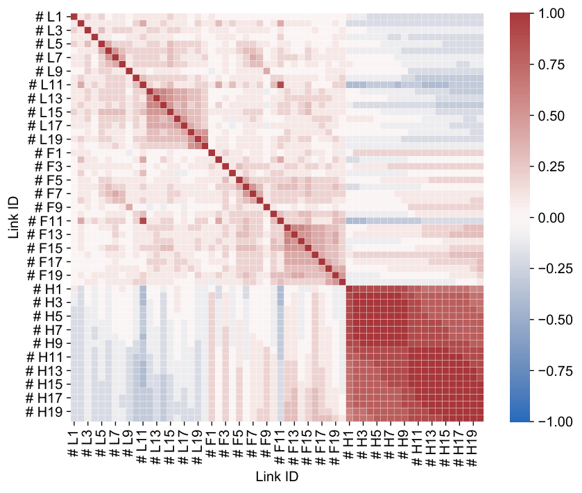
Moreover, Fig. 9 depicts the correlation matrices for different clusters/patterns. Both of the correlation matrices show the complex characteristics of the correlations between link travel times/headways: 1) long-range correlations, 2) negative correlations, and 3) different patterns. On the other hand, it also shows clear differences between correlation matrices of different clusters. The most significant difference is that the leading bus and the following bus for cluster 1 could be more correlated than that for cluster 2. Therefore, characterizing the bus travel time with a Gaussian mixture model is of great significance in practice.

We show the application of the probabilistic forecasting model for bus route No.60 of a selected day in Fig. 10. The left panel intuitively illustrates the probabilistic forecasting for bus travel time at 16:50 p.m., while the right panel corresponds to the forecasting at 17:10 p.m. All actual bus operations are shown by green lines in the time-space diagram. Assume that past operation of buses (i.e., before 16:50 p.m. and before 17:10 p.m.) are observed and we use the observed information to forecast the future time-space position of buses. The variability of the probabilistic forecasting is shown with the 10th, 25th, 40th, 60th, 75th, and 90th percentile values. We can see that the proposed model can make a good probabilistic forecasting for bus arrival time. By comparing the two figures, we can also find that for a bus trip, more observed links can help improve the forecasting accuracy and reduce the forecasting variability.

Finally, we use the two bus trips to show the forecasting distributions. Fig. 11 shows the probabilistic forecasting results. In this experiment, we assume that we have observed the first eleven link travel times of the following bus and the corresponding link travel times/headways of the leading bus, then we intend to make probabilistic forecasting for the trip travel times of the last several links. In the left panel, the brown points are the trip travel times of the leading bus; the blue points are the true trip travel times of the following bus, and the green points are the predictive mean values. We can see that the predictive mean values fit the actual values quite well, demonstrating the proposed probabilistic model can achieve accurate forecasts. Moreover, the red bell curves are the trip travel time distributions, and we can find that the red bell curves are fatter with the increasing number of links in a trip, indicating the variance is increasing. The right panels show the mean corrected estimation, and the purple points (we refer to them as corrected mean values) are computed by posterior conditional mean values minus model mean values; the orange points are computed by the difference between true values and model mean values. We can find that the posterior conditional mean can make a more accurate prediction than the model mean. If we do not use the information of the observed link travel times/headways, the forecasting mean vectors should be the model mean vectors. As can be seen, the corrected mean values for observation 1 as shown in Fig. 11 (a) are larger than zero, while the corrected mean values for observation 2 as shown in Fig. 11 (b) are lower than zero, demonstrating the observed information indeed reinforces the forecasting for the upcoming links.

References

- Alam et al. (2021) Alam, O., Kush, A., Emami, A., Pouladzadeh, P., 2021. Predicting irregularities in arrival times for transit buses with recurrent neural networks using gps coordinates and weather data. Journal of Ambient Intelligence and Humanized Computing 12 (7), 7813–7826.
- Bai et al. (2015) Bai, C., Peng, Z.-R., Lu, Q.-C., Sun, J., 2015. Dynamic bus travel time prediction models on road with multiple bus routes. Computational intelligence and neuroscience 2015.
- Bin et al. (2006) Bin, Y., Zhongzhen, Y., Baozhen, Y., 2006. Bus arrival time prediction using support vector machines. Journal of Intelligent Transportation Systems 10 (4), 151–158.
- Blei et al. (2003) Blei, D. M., Ng, A. Y., Jordan, M. I., 2003. Latent dirichlet allocation. Journal of machine Learning research 3 (Jan), 993–1022.
- Büchel and Corman (2018) Büchel, B., Corman, F., 2018. Modelling probability distributions of public transport travel time components. In: 18th Swiss Transport Research Conference (STRC 2018). STRC.
- Büchel and Corman (2020) Büchel, B., Corman, F., 2020. Review on statistical modeling of travel time variability for road-based public transport. Frontiers in Built Environment 6, 70.
- Büchel and Corman (2022a) Büchel, B., Corman, F., 2022a. Modeling conditional dependencies for bus travel time estimation. Physica A: Statistical Mechanics and Its Applications 592, 126764.
- Büchel and Corman (2022b) Büchel, B., Corman, F., 2022b. What do we know when? modeling predictability of transit operations. IEEE Transactions on Intelligent Transportation Systems.
- Cathey and Dailey (2003) Cathey, F., Dailey, D. J., 2003. A prescription for transit arrival/departure prediction using automatic vehicle location data. Transportation Research Part C: Emerging Technologies 11 (3-4), 241–264.
- Cats and Gkioulou (2017) Cats, O., Gkioulou, Z., 2017. Modeling the impacts of public transport reliability and travel information on passengers’ waiting-time uncertainty. EURO Journal on Transportation and Logistics 6 (3), 247–270.
- Chen et al. (2004) Chen, M., Liu, X., Xia, J., Chien, S. I., 2004. A dynamic bus-arrival time prediction model based on apc data. Computer-Aided Civil and Infrastructure Engineering 19 (5), 364–376.
- Chen et al. (2022) Chen, X., Cheng, Z., Sun, L., 2022. Bayesian inference for link travel time correlation of a bus route. arXiv preprint arXiv:2202.09485.
- Chepuri et al. (2020) Chepuri, A., Joshi, S., Arkatkar, S., Joshi, G., Bhaskar, A., 2020. Development of new reliability measure for bus routes using trajectory data. Transportation Letters 12 (6), 363–374.
- Chien et al. (2002) Chien, S. I.-J., Ding, Y., Wei, C., 2002. Dynamic bus arrival time prediction with artificial neural networks. Journal of transportation engineering 128 (5), 429–438.
- Cong et al. (2017) Cong, Y., Chen, B., Zhou, M., 2017. Fast simulation of hyperplane-truncated multivariate normal distributions. Bayesian Analysis 12 (4), 1017–1037.
- Dai et al. (2019) Dai, Z., Ma, X., Chen, X., 2019. Bus travel time modelling using gps probe and smart card data: A probabilistic approach considering link travel time and station dwell time. Journal of Intelligent Transportation Systems 23 (2), 175–190.
- Farhan et al. (2002) Farhan, A., Shalaby, A., Sayed, T., 2002. Bus travel time prediction using avl and apc. In: Applications of Advanced Technologies in Transportation (2002). pp. 616–623.
- Gelman et al. (2013) Gelman, A., Carlin, J. B., Stern, H. S., Dunson, D. B., Vehtari, A., Rubin, D. B., 2013. Bayesian Data Analysis, 3rd Edition. Chapman and Hall/CRC.
- Gurmu and Fan (2014) Gurmu, Z. K., Fan, W. D., 2014. Artificial neural network travel time prediction model for buses using only gps data. Journal of Public Transportation 17 (2), 3.
- Harsha and Mulangi (2021) Harsha, M., Mulangi, R. H., 2021. Probability distributions analysis of travel time variability for the public transit system. International Journal of Transportation Science and Technology.
- He et al. (2020) He, P., Jiang, G., Lam, S.-K., Sun, Y., 2020. Learning heterogeneous traffic patterns for travel time prediction of bus journeys. Information Sciences 512, 1394–1406.
- Huang et al. (2021) Huang, Y., Chen, C., Su, Z., Chen, T., Sumalee, A., Pan, T., Zhong, R., 2021. Bus arrival time prediction and reliability analysis: An experimental comparison of functional data analysis and bayesian support vector regression. Applied Soft Computing 111, 107663.
- Jeong and Rilett (2004) Jeong, R., Rilett, R., 2004. Bus arrival time prediction using artificial neural network model. In: Proceedings. The 7th international IEEE conference on intelligent transportation systems (IEEE Cat. No. 04TH8749). IEEE, pp. 988–993.
- Kieu et al. (2015) Kieu, L.-M., Bhaskar, A., Chung, E., 2015. Public transport travel-time variability definitions and monitoring. Journal of Transportation Engineering 141 (1), 04014068.
- Kumar et al. (2018) Kumar, B. A., Vanajakshi, L., Subramanian, S. C., 2018. A hybrid model based method for bus travel time estimation. Journal of Intelligent Transportation Systems 22 (5), 390–406.
- Lam and Small (2001) Lam, T. C., Small, K. A., 2001. The value of time and reliability: measurement from a value pricing experiment. Transportation Research Part E: Logistics and Transportation Review 37 (2-3), 231–251.
- Ma et al. (2019) Ma, J., Chan, J., Ristanoski, G., Rajasegarar, S., Leckie, C., 2019. Bus travel time prediction with real-time traffic information. Transportation Research Part C: Emerging Technologies 105, 536–549.
- Ma et al. (2016) Ma, Z., Ferreira, L., Mesbah, M., Zhu, S., 2016. Modeling distributions of travel time variability for bus operations. Journal of Advanced Transportation 50 (1), 6–24.
- Ma et al. (2017) Ma, Z., Koutsopoulos, H. N., Ferreira, L., Mesbah, M., 2017. Estimation of trip travel time distribution using a generalized markov chain approach. Transportation Research Part C: Emerging Technologies 74, 1–21.
- Madzlan et al. (2010) Madzlan, N., Ibrahim, K., et al., 2010. Arima models for bus travel time prediction.
- Mazloumi et al. (2010) Mazloumi, E., Currie, G., Rose, G., 2010. Using gps data to gain insight into public transport travel time variability. Journal of transportation engineering 136 (7), 623–631.
- Osman et al. (2021) Osman, O., Rakha, H., Mittal, A., 2021. Application of long short term memory networks for long-and short-term bus travel time prediction.
- Petersen et al. (2019) Petersen, N. C., Rodrigues, F., Pereira, F. C., 2019. Multi-output bus travel time prediction with convolutional lstm neural network. Expert Systems with Applications 120, 426–435.
- Rahman et al. (2018) Rahman, M. M., Wirasinghe, S., Kattan, L., 2018. Analysis of bus travel time distributions for varying horizons and real-time applications. Transportation Research Part C: Emerging Technologies 86, 453–466.
- Ricard et al. (2022) Ricard, L., Desaulniers, G., Lodi, A., Rousseau, L.-M., 2022. Predicting the probability distribution of bus travel time to measure the reliability of public transport services. Transportation Research Part C: Emerging Technologies 138, 103619.
- Taylor (1982) Taylor, M., 1982. Travel time variability—the case of two public modes. Transportation Science 16 (4), 507–521.
- Uno et al. (2009) Uno, N., Kurauchi, F., Tamura, H., Iida, Y., 2009. Using bus probe data for analysis of travel time variability. Journal of Intelligent Transportation Systems 13 (1), 2–15.
- Xu and Ying (2017) Xu, H., Ying, J., 2017. Bus arrival time prediction with real-time and historic data. Cluster Computing 20 (4), 3099–3106.
- Yang et al. (2016) Yang, M., Chen, C., Wang, L., Yan, X., Zhou, L., 2016. Bus arrival time prediction using support vector machine with genetic algorithm. Neural Network World 26 (3), 205.
- Yetiskul and Senbil (2012) Yetiskul, E., Senbil, M., 2012. Public bus transit travel-time variability in ankara (turkey). Transport Policy 23, 50–59.
- Yu et al. (2011) Yu, B., Lam, W. H., Tam, M. L., 2011. Bus arrival time prediction at bus stop with multiple routes. Transportation Research Part C: Emerging Technologies 19 (6), 1157–1170.
- Yu et al. (2018) Yu, B., Wang, H., Shan, W., Yao, B., 2018. Prediction of bus travel time using random forests based on near neighbors. Computer-Aided Civil and Infrastructure Engineering 33 (4), 333–350.
- Zhang et al. (2021) Zhang, X., Yan, M., Xie, B., Yang, H., Ma, H., 2021. An automatic real-time bus schedule redesign method based on bus arrival time prediction. Advanced Engineering Informatics 48, 101295.