Searches for Continuous-Wave Gravitational RadiationJournal: Living Reviews in Relativity
Abstract
Now that detection of gravitational wave signals from the coalescence of extra-galactic compact binary star mergers has become nearly routine, it is intriguing to consider other potential gravitational wave signatures. Here we examine the prospects for discovery of continuous gravitational waves from fast-spinning neutron stars in our own galaxy and from more exotic sources. Potential continuous-wave sources are reviewed, search methodologies and results presented and prospects for imminent discovery discussed.
1 Introduction
The LIGO (Aasi et al. 2015a) and Virgo (Acernese et al. 2014) gravitational wave detectors have made historic discoveries over the last seven years. The first direct detection in September 2015 of gravitational waves marked a milestone in fundamental science (Abbott et al. 2016b), confirming a longstanding prediction of Einstein’s General Theory of Relativity (Einstein 1916; Einstein 1918). That the detection came from the first observation of a binary black hole merger provided a bonus not only in verifying detailed predictions of General Relativity, but in establishing unambiguously that stellar-mass black holes exist in the Universe. More than 80 binary black hole (BBH) systems have been observed since GW150914 (Abbott et al. 2016d; Abbott et al. 2017h; Abbott et al. 2017i; Abbott et al. 2017j; Abbott et al. 2019b; Abbott et al. 2021e; Abbott et al. 2021f). Merging binary neutron star (BNS) systems (Abbott et al. 2017k; Abbott et al. 2020a) have also been observed, including GW170817 (Abbott et al. 2017k), which was accompanied by a multitude of electromagnetic observations (Abbott et al. 2017l). Those observations confirmed the association of at least some short gamma ray bursts with binary neutron star mergers (Abbott et al. 2017g) and the onset of kilonovae in BNS mergers that contribute substantially to the heavy element production in the Universe (Abbott et al. 2017l). More recently came detections of merging neutron star – black hole (NSBH) systems (Abbott et al. 2021g). These discoveries of transient gravitational wave signals have ignited the field of gravitational wave astronomy.
This review concerns a quite different and as-yet-undiscovered gravitational wave signal type, one defined by stability and near-monochromaticity over long time scales, namely continuous waves. CW signals with strengths detectable by current and imminent ground-based gravitational wave interferometers could originate from relatively nearby galactic sources, such as fast-spinning neutron stars exhibiting non-axisymmetry (Thorne 1989), or more exotically, from strong extra-galactic sources, such as super-radiant Bose-Einstein clouds surrounding black holes (Arvanitaki et al. 2010).
We already know from prior LIGO and Virgo searches that the strengths of CW signals must be exceedingly weak [ or less], which is consistent with theoretical expectation, from which we expect plausible CW strain amplitudes to be orders of magnitudes lower than the amplitudes of the transient signals detected to date []. This disparity in signal strength holds despite the much nearer distance of galactic neutron stars (kpc) compared to the compact binary mergers (40 Mpc to multi-Gpc) seen to date. In fact, it is only their long-lived nature that gives us any hope of detecting CW signals through integration over long data spans, so as to achieve a statistically viable signal-to-noise (SNR) ratio. As discussed below, however, that SNR increases, at best, as the square root of observation time, but for most CW searches, increases with an even lower power of observation time, while computational cost increases with much higher powers. These different scalings of signal sensitivity and cost have led to a variety of approaches in targeting signals, depending on the size of signal parameter space searched.
The search for continuous gravitational radiation has been under way since the 1970’s, using data from interferometers (Levine and Stebbins 1972) and bars (Hirakawa et al. 1978; Suzuki 1995), including from early prototypes (Livas 1989) for the large gravitational wave detectors to come later. This review focuses primarily on the most recent searches from the Advanced LIGO and Virgo detectors, although summaries of search algorithm developments in the initial LIGO and Virgo era (and before) provide some historical context. For reference, the Advanced LIGO and Virgo runs to date comprise (with selected highlighted detections):
- •
The O1 observing run (LIGO only): September 12, 2015 – January 12, 2016 – First detection of gravitational waves from a BBH merger: GW150914 (Abbott et al. 2016b).
- •
The O2 observing run (LIGO joined by Virgo in last month): November 30, 2016 – August 25, 2017 – First detection of gravitational waves from a BNS merger: GW170817 (Abbott et al. 2017k).
- •
The O3 observing run (LIGO and Virgo): April 1, 2019 – March 27, 2020 – First detection of gravitational waves from the formation of an intermediate-mass black hole: GW190521 (Abbott et al. 2020d) and the first detection of NSBH mergers. The run was divided into a 6-month “O3a” epoch (April 1, 2019 – October 1, 2019) and “O3b” (November 1 – March 27, 2020) by a 1-month commissioning break. Many initial publications focused on results from the O3a data.
In the following, section 2 reviews both conventional and exotic potential sources of CW gravitational radiation. Section 3 describes a wide variety of search methodologies being used to address the challenges of detection. Section 4 presents results (so far only upper limits) from searches based on these algorithms, with an emphasis on the most recent results from the Advanced LIGO and Virgo detectors. Finally, section 5 discusses the outlook for discovery in the coming years, including the prospects for electromagnetic observations of the continuous gravitational wave sources. This review focuses on CW radiation potentially detectable with current-generation and next-generation ground-based gravitational wave interferometers, which are sensitive to gravitational frequencies in the human-audible band for sound. Past and future searches for lower-frequency CW radiation from supermassive black hole binaries at nHz frequencies using pulsar timing arrays (Manchester 2010) or from stellar-mass galactic binaries at mHz frequencies using the space-based LISA (Bender et al. 1996) are not discussed here.
Textbooks addressing gravitational waves, their detection and their analysis include Misner et al. 1972; Schutz 1985; Maggiore 2008; Maggiore 2018; Saulson 2017; Creighton and Anderson 2011; Jaranowski and Królak 2009; Andersson 2019. Review articles and volumes on gravitational wave science include Thorne 1989; Blair et al. 1991; Sathyaprakash and Schutz 2009; Pitkin et al. 2011; Freise and Strain 2010; Blair et al. 2012; Riles 2013; Romano and Cornish 2017. This review is a substantial expansion upon a briefer previous article (Riles 2017). Other reviews of CW search methodology include Prix 2009; Palomba 2012; Lasky 2015; Sieniawska and Bejger 2019; Tenorio et al. 2021b; Piccinni 2022.
2 Potential sources of CW radiation
In the frequency band of present ground-based detectors, the canonical sources of continuous gravitational waves are galactic, non-axisymmetric neutron stars spinning fast enough to produce gravitational waves in the LIGO and Virgo detectable band (at 1, 4/3 or 2 rotation frequency, depending on the generation mechanism). These nearby neutron stars offer a “conventional” source of CW radiation – as astrophysically extreme as such objects are.
A truly exotic postulated source is a “cloud” of bosons, such as QCD axions, surrounding a fast-spinning black hole, bosons that can condense in gargantuan numbers to a small number of discrete energy levels, enabling coherent gravitation wave emission from boson annihilation or from level transitions. Attention here focuses mainly on the conventional neutron stars, but the exotic boson cloud scenario is also discussed.
2.1 Fast-spinning neutron stars
The following subsections give an overview of neutron star formation, structure, observables and populations, present the phenomenology of neutron-star spin-down, discuss potential sources of non-axisymmetry in neutron stars, and consider a number of particular GW search targets of interest. Although neutron stars were first postulated by Baade & Zwicky (Baade and Zwicky 1934) and their basic properties worked out by Oppenheimer and Volkoff (Oppenheimer and Volkoff 1939), the first definitive establishment of their existence came with the discovery of the first radio pulsar (Hewish et al. 1968) PSR B1919+21 in 1967 with prior theoretical support for neutron star radiation contributing to supernova remnant shell energetics (Pacini 1967) and rapid theoretical follow-up to explain the pulsation mechanism (Gold 1968; Goldreich and Julian 1969; Ruderman and Sutherland 1975).
2.1.1 Neutron star formation, structure, observables and populations
As background, this section surveys at a basic level the fundamentals of neutron star formation, structure, observables and populations. Much more detailed information can be found in the following review articles or volumes on neutron stars (Lattimer and Prakash 2001; Chamel and Haensel 2008; Becker 2009; Özel and Freire 2016), pulsars (Lorimer and Kramer 2005; Lyne and Graham-Smith 2006; Lorimer 2008), and rotating relativistic stars (Paschalidis and Stergioulas 2017).
Neutron stars are the final states of stars too massive to form white dwarfs upon collapse after fuel consumption and too light to form black holes, having progenitor masses in the approximate range 6–15 (Lyne and Graham-Smith 2006; Cerda-Duran and Elias-Rosa 2018; Stockinger et al. 2020). These remarkably dense objects, supported by neutron degeneracy pressure, boast near-nuclear densities in their crusts and well-beyond-nuclear densities in their cores. The range of densities and associated total stellar masses and radii depend on an equation of state that is not experimentally accessible in terrestrial laboratories because of the combination of high density and (relatively) low temperature. A variety of equations of state have been proposed (Lattimer and Prakash 2001), with a small subset disfavored by the measurement of neutron stars greater than two solar masses (Buballa et al. 2014), by radii of approximately ten kilometers (Miller et al. 2019b; Miller et al. 2021; Riley et al. 2019; Riley et al. 2021) and by the absence of severe tidal deformation effects in the gravitational waveforms measured for the BNS merger GW170817 (Abbott et al. 2017k; Abbott et al. 2018c; Lim and Holt 2019; Essick et al. 2020). The detection of a 2.6- object in the GW190814 merger (Abbott et al. 2020e) poses a challenge to the nuclear equation of state if the object is indeed a neutron star instead of a light black hole.
In broad summary, a neutron star is thought to have a crust with outer radius between 10 and 15 km and a thickness of 1 km (Shapiro and Teukolsky 1983), composed near the top of a tight lattice of neutron-rich heavy nuclei, permeated by neutron superfluid. Deeper in the star, as pressure and density increase, the nuclei may become distorted and elongated, forming a “nuclear pasta” of ordered nuclei and gaps (Ravenhall et al. 1983; Caplan and Horowitz 2017). Still deeper, the pasta gives way to a hyperdense neutron fluid and perhaps undergoes phase transitions involving hyperons, perhaps to a quark-gluon plasma, or even perhaps to a solid strange-quark core (Shapiro and Teukolsky 1983; Lattimer and Prakash 2001).
Uncertainties in equation of state lead directly to uncertainties in the expected maximum mass and radius of a neutron star (Lattimer and Prakash 2001), but theoretical prejudice is consistent with the absence of observation in binary systems of neutron star masses much higher than two solar masses (Özel and Freire 2016; Demorest et al. 2010; Arzoumanian et al. 2018; Antoniadis et al. 2013; Cromartie et al. 2020; Fonseca et al. 2021). Neutron star radii are especially challenging to measure directly, with older measurements coming from X-ray measurements, where inferences are drawn from brightness of the radiation, its temperature and distance to the source, assuming black-body radiation, with corrections for the strong space-time curvature affecting the visible surface area (Özel and Freire 2016; Degenaar and Suleimanov 2018). New measurements from the NICER X-ray satellite are improving upon the precision with which mass and radius can be determined simultaneously from individual stars, constraining more tightly the allowed equations of state (Miller et al. 2019b; Miller et al. 2021; Bogdanov et al. 2019a; Bogdanov et al. 2019b; Bogdanov et al. 2021; Raaijmakers et al. 2019; Raaijmakers et al. 2021; Riley et al. 2019; Riley et al. 2021).
Measurements of the gravitational waveform from the binary neutron star merger GW170817 have also provided new constraints and disfavor very stiff equations of state that lead to large neutron star radii (Abbott et al. 2018c). Detection of additional binary neutron star mergers in the coming years should improve these constraints. Broadly, one expects average neutron star densities of g cm-3, well above the density of nuclear matter () (Lorimer and Kramer 2005), with densities at the core likely above g cm-3 (Shapiro and Teukolsky 1983). See (Yunes et al. 2022) for a recent review of what has been learned about the neutron star equation of state from gravitational wave and X-ray observations. A recent Bayesian combined analysis (Huth et al. 2022) of predictions from chiral effective field theory of QCD, measured BNS gravitational waveforms, NICER X-ray observations and measurements from heavy ion (gold) collisions indicate a somewhat stiffer equation of state than previously favored and hence larger allowed radii of neutron stars.
Given the immense pressure on the nuclear matter, one expects a neutron star to assume a highly spherical shape in the limit of no rotation and, with rotation, to become an axisymmetric oblate spheroid. True axisymmetry would preclude emission of quadrupolar gravitational waves from rotation alone. Hence CW searchers count upon a small but detectable mass (or mass current) non-axisymmetry, discussed in detail in section 2.1.3.
During the collapse of their slow-spinning stellar progenitors, neutron stars can acquire an impressive rotational speed as angular momentum conservation spins up the infalling matter. Even the two slowest-rotating known pulsars spin on their axes every 76 seconds (Caleb et al. 2022) and 24 seconds (Tan et al. 2018; Manchester and Hobbs 2005), implying rotational kinetic energies greater than J, and other young pulsars with spin frequencies of 10’s of Hz have rotational energies of J. Recycled millisecond pulsars acquire even higher spins via accretion from a binary companion star, leading to measured spin frequencies above 700 Hz (Hessels et al. 2006; Bassa et al. 2017) and a rotational energy of J, or several percent of the magnitude of the gravitational bound energy of the star. This immense reservoir of rotational energy might appear to bode well for supporting detectable gravitational wave emission, but vast energy is required to create appreciable distortions in highly rigid space-time. From the perspective of gravitational-wave energy density (Misner et al. 1972), one can define an effective, frequency-dependent Young’s modulus ( Pa for Hz, or 20 orders of magnitude higher than steel). As a result, one must tap a significant fraction of the reservoir’s energy loss rate in order to produce detectable radiation, as quantified below.
Most of the 3300 known neutron stars in the galaxy are pulsars, detected via pulsed electromagnetic emission, primarily in the radio band, but also in X-rays and -rays (with a small number detected optically) (Lyne and Graham-Smith 2006; Manchester and Hobbs 2005). Pulses are typically observed at the rotation frequency of the star, as a beam of radiation created by curvature radiation (Buschauer and Benford 1976) from particles that are flung out in a plasma from the magnetic poles (misaligned with the spin axis) and accelerated transversely by the magnetic field, sweeps across the Earth once per rotation (see (Melrose et al. 2021), however, for a critique of this model). A subset of neutron stars presumed to have magnetic poles tilted nearly 90 degrees from the spin axis display two distinct pulses.
Other neutron stars are known from detection of X-rays from thermal emission (heat from formation and perhaps from magnetic field decay), particularly at sites consistent with the birth locations and times of supernova remnants (Lyne and Graham-Smith 2006). Still other neutron stars are inferred from accretion X-rays observed in binary systems, particularly low-mass X-ray binaries with accretion disks (Lyne and Graham-Smith 2006), although some accreting binaries with compact stars contain black holes, such as the high-mass X-ray binary Cygnus X-1. Figure 1 shows nearly the entire population of currently known pulsars (Manchester and Hobbs 2005) with spin period shorter than 20 seconds11 1 The longest known pulsation period is 76f seconds from the recently discovered PSR J0901-4046 (Caleb et al. 2022), which also displays unusual pulse length and variability and which may represent a new pulsar class. in the – plane, where is the first time derivative of the period. Red triangles show isolated pulsars, and blue circles show binary pulsars.

Neutron stars have strong magnetic field intensities as a natural result of their collapse. If the magnetic flux is approximately conserved, the reduction of the outer surface of the star to a radius of 10 km ensures a static surface field far higher than achievable in a terrestrial laboratory (Pacini 1967), with inferred values (see below) ranging from G to more than G (Lyne and Graham-Smith 2006). The strongest fields are seen in so-called “magnetars,” young neutron stars with extremly rapid spin-down, for which dynamo generation is also likely relevant (Guilet and Müller 2015; Mösta et al. 2015). Both in young pulsars and in binary millisecond pulsars, there is reason to believe that stronger magnetic fields are “buried” in the star from accreting plasma (Payne and Melatos 2004), although the burial mechanism is not confidently understood (Chevalier 1989; Geppert et al. 1999; Lyne and Graham-Smith 2006; Bernal et al. 2010). It has been suggested there is evidence in at least some pulsars for slowly re-emerging (strengthening) magnetic field (Ho 2011; Espinoza et al. 2011). Energy density deformation from a potentially non-axisymmetric buried field is another potential source of GW emission (Bonazzola and Gourgoulhon 1996). See (Cruces et al. 2019) for a discussion of magnetic field decay preceding the accretion stage.
In principle, there should be neutron stars in our galaxy, (Narayan 1987; Treves et al. 2000). That only a small fraction have been detected is expected, for several reasons. Radio pulsations require high magnetic field and rotation frequency. Early studies (Goldreich and Julian 1969; Sturrock 1970; Ruderman and Sutherland 1975; Lorimer and Kramer 2005) implied the relation
| (1) |
based on a model of radiation dominated by electron-positron pair creation in the stellar magnetosphere, a model broadly consistent with empirical observation, although the resulting “death line” (see Figure 1) in the plane of period and period derivative is perhaps better understood to be a valley (Chen and Ruderman 1993; Zhang et al. 2000; Beskin and Litvinov 2022; Beskin and Istomin 2022).
The death line can be understood qualitatively from the following argument. The rotating magnetic field of a neutron star creates a strong electric field that pulls charged particles from the star, forming a plasma with charge density that satisfies (SI units): (Chen and Ruderman 1993)
| (2) | |||||
| (3) |
where is the angular velocity of the star, and is the local magnetic field at location with respect to the star’s center. In steady-state equilibrium, one expects since free charges can move along -field lines. In so-called “gaps,” however, where the plasma density is low, a potential difference large enough to produce spontaneous electron-positron pair production can lead to radio-frequency synchrotron radiation as the accelerated particles encounter curved magnetic fields. This emission is thought to account for most radio pulsations (Lyne and Graham-Smith 2006), where an “inner gap” refers to a region just outside the magnetic poles above the star’s surface, and an “outer gap” refers to a region where a nominally dipolar magnetic field is approximately perpendicular to the rotation direction, separating regions of proton and electron flow from the star to the region beyond the “light cylinder,” defined by the cylindrical radius at which a co-rotating particle in the magnetosphere must travel at the speed of light. For the inner gap to have a voltage drop high enough to induce an amplifying cascade of pair production leading to coherent radio wave emission imposes a minimum value on the gap potential difference which, in general, can be approximated by (SI units): (Goldreich and Julian 1969; Sturrock 1970; Ruderman and Sutherland 1975; Chen and Ruderman 1993)
| (4) |
where is the neutron star radius, leading (in a more detailed calculation) to Eqn. 1 and via magnetic dipole emission assumptions (see section 2.1.2) to the death line shown in Figure 1 (but see (Smith et al. 2019) for evidence of selection effects and (Pétri 2019) for a discussion of potentially important effects from higher order multipoles). Presumably, the vast majority of neutron stars created in the galaxy’s existence to date are now to the right of the line. Additional negative-sloped dashed lines in the figure indicate different nominal magnetic dipole field strengths and positive-sloped dashed lines indicate different nominal ages, based on observed present-day periods and period derivatives (see section 2.1.2).
Two distinct major pulsar populations are apparent in Figure 1, defined by location in the diagram. The bulk of the population lies above and to the right of the line corresponding to G. The bulk also lies above and to the left of the line corresponding to ages younger than years. Assuming a star’s magnetic field strength is stable, stars are expected to migrate down to the right along the -field contours. Isolated pulsars seem to have typical pulsation lifetimes of years (Lyne and Graham-Smith 2006), after which they become increasingly difficult to observe in radio. On this timescale, they also cool to where thermal X-ray emission is difficult to detect (Potekhin et al. 2015). There remains the possibility of X-ray emission from steady accretion of interstellar medium (ISM) (Ostriker et al. 1970; Blaes and Madau 1993), but it appears that the kick velocities from birth highly suppress such accretion (Hoyle and Lyttleton 1939; Bondi and Hoyle 1944) which depends on the inverse cube of the star’s velocity through the ISM, and steady-state X-ray emission from accretion onto even slow-moving neutron stars can be highly suppressed, consistent with non-observation to date of such accretion (Popov et al. 2015).
The remaining population, in the lower left of the figure, is characterized by shorter periods and smaller period derivatives. These are so-called “millisecond pulsars” (MSPs), thought to arise from “recycling” of rotation speed due to accretion of matter from a binary companion. MSPs are stellar zombies, brought back from the dead with immense rotational energies imparted by infalling matter (Alpar et al. 1982; Radhakrishnan and Srinivasan 1982). The rotation frequencies achievable through this spin-up are impressive – the fastest known rotator is PSR J17482446ad at 716 Hz (Hessels et al. 2006). One progenitor class for MSPs is the set of low mass X-ray binaries (LMXBs) in which the neutron star (1.4 ) has a much lighter companion (0.3 ) (Lyne and Graham-Smith 2006) that overfills its Roche lobe, spilling material onto an accretion disk surrounding the neutron star or possibly spilling material directly onto the star, near its magnetic polar caps. When the donor companion star eventually shrinks and decouples from the neutron star, the neutron star can retain a large fraction of its maximum angular momentum and rotational energy. Because the neutron star’s magnetic field decreases during accretion (through processes that are not well understood), the spin-down rate after decoupling can be very small. The minority of MSPs that are isolated are thought to have lost their one-time companions via consumption and ablation. A bridging class called “black widows” and “redbacks” refer to binary systems with actively ablating companions, such as B1957+20 (Fruchter et al. 1988; Strader et al. 2019; Roberts and van Leeuwen 2013), where black widows denote the extreme subclass with companion masses below 0.1 (Roberts and van Leeuwen 2013).
A nice confirmation of the link between LMXBs and recycled MSPs comes from “transitional millisecond pulsars” (tMSPs) in which accreting LMXB behavior alternates with detectable radio pulsations. The first tMSP found was PSR J10230038 (Bond et al. 2002; Thorstensen and Armstrong 2005; Archibald et al. 2009), with two more systems since detected (Jaodand et al. 2017). The nominal ages of MSPs extend beyond 1010 years, that is, some have apparent ages greater than that of the galaxy (or even that of the Universe). One possible explanation of this anomaly is reverse-torque spin-down during the Roche decoupling phase (Tauris 2012), although a recent numerical study suggests a more complex frequency evolution before and during the decoupling (Bhattacharyya 2021).
An obvious pattern in Figure 1, consistent with the recycling model, is the higher fraction of binary systems at lower periods. For example, binary systems account for 3/4 of the lowest 200 pulsar periods (below 4 ms).
Aside from the disappearance of stars from this diagram as they evolve toward the lower right and cease pulsations, there are also strong selection effects that suppress the visible population. We observe pulsars only if their radiation beams cross the Earth, only if that radiation is bright enough to be seen in the observing band, and only if the radiation is not sufficiently absorbed, scattered or frequency-dispersed to prevent detection with current radio telescopes. When the Square Kilometer Array project comes to fruition in the late 2020’s, it is estimated that the current known population of pulsars will grow tenfold (Kramer and Stappers 2015).
2.1.2 Neutron star spin-down phenomenology and mechanisms
Nearly every known pulsar is observed to be spinning down, that is, to have a negative rotational frequency time derivative, implying loss of rotational kinetic energy. As discussed below in detail, there are many physical mechanisms, electromagnetic and gravitational, that can lead to this energy loss. For CW signal detection we want a gravitational wave component, but there is good reason to believe that electromagnetic processes dominate for nearly every known pulsar.
A convenient and commonly used phenomenological model for spin-down is a power law:
| (5) |
where is the star’s instantaneous frequency (rotational or gravitational: ), is the first time derivative, and is a negative constant for all but a handful of stars (thought to be experiencing large acceleration toward us because of nearness to a deep gravitational well, such as in the core of a globular cluster). The exponent depends on the spin-down mechanism and is known as the braking index. The four most common theoretical braking indices discussed in the literature are the following:
- •
– “Pulsar wind” (extreme model)
- •
– Magnetic dipole radiation
- •
– Gravitational mass quadrupole radiation (“mountain”)
- •
– Gravitational mass current quadrupole radiation (-modes).
In principle, other oscillation modes that can generate gravitational waves are also possible, but the and modes discussed below are thought to be the most promising.
Assuming the same power law has applied since the birth of the star, the age of the star can be related to its birth rotation frequency and current frequency by ():
| (6) |
and in the case that ,
| (7) |
A common baseline assumption in radio pulsar astronomy is that the braking index is from which the nominal magnetic dipole age of a star can be defined
| (8) |
again, under the assumption .
From the more generic power-law spin-down model (Eqn. 5), the 2nd frequency derivative can be written:
| (9) |
from which the current braking index can be determined if the spin frequency’s 2nd time derivative can be measured reliably:
| (10) |
Before examining the empirical measurements of the braking indices, which are mostly inconsistent with , let’s briefly review spin-down mechanisms with well defined braking indices, when dominant. For GW radiation spin-down dominance, related “spin-down” limits on strain amplitude will also be presented.
2.1.2.1 “Pulsar wind” ().
Early on in pulsar astronomy (Michel 1969; Michel and Tucker 1969) it was recognized that the streaming of relativistic particles (electrons and positrons mainly, with some ions) away from the magnetosphere of a fast-spinning neutron star would lead to a spin-down torque that could, in principle, rival that from magnetic dipole radiation, in addition to distorting the shape of the magnetic field lines and affecting the dipole radiation (Gaensler and Slane 2006). In this perhaps too-simple model, the spin-down is dominated by a braking torque from a return current (predominantly counter-flowing electrons and positrons) crossing magnetic field lines in the polar cap regions of the star (Contopoulos et al. 1999), leading to a braking index of one. A more recent study of magnetar spin-down (Harding et al. 1999) considered a model with sporadic high winds following bursts, with magnetic dipole emission dominating spin-down between bursts. In the steady state, however, considering the interaction of the magnetic field and the plasma of the magnetosphere, both magnetic dipole emission and pulsar wind contributions tend to yield a braking index of about three (Michel and Li 1999; Spitkovsky 2004), discussed next. A phenomenological model (Melatos 1997) that is a variant of the vacuum dipole mode, featuring an inner magnetosphere strongly coupled to the star, accounts successfully for the braking indices of the Crab and other young pulsars with .
2.1.2.2 Magnetic dipole ().
The radiation energy loss due to a rotating magnetic dipole moment is (Pacini 1968)
| (11) |
where is the rotational angular speed and is the component of the star’s magnetic dipole moment perpendicular to the rotation axis (taken to be the axis): , with the angle between the axis and north magnetic pole.
In a pure dipole moment model, the magnetic pole field strength at the surface is . Equating the radiation energy loss to that of the (Newtonian) rotational energy leads to the prediction:
| (12) |
Hence the magnetic dipole spin-down rate is proportional to the square of and to the cube of the rotation frequency, giving .
2.1.2.3 Gravitational mass quadrupole (“mountain”, ).
Let’s now consider the gravitational radiation one might expect from these stars. It is conventional to characterize a star’s mass quadrupole asymmetry by its equatorial ellipticity:
| (13) |
An oblate spheroid naturally has a polar ellipticity, but in the absence of precession22 2 Free precession of an oblate neutron star can lead to gravitational radiation at the rotation frequency (Zimmermann and Szedenits 1979), but there is little empirical evidence for such precession in pulsars and good reason to expect that such precession would be rapidly damped by internal dissipation (Jones and Andersson 2002)., such a deformation does not lead to GW emission. Henceforth “ellipticity” will refer to equatorial ellipticity, often attributed to a “mountain”. For a star at a distance away and spinning about the approximate symmetry axis of rotation (), (assumed optimal – pointing toward the Earth), then the expected intrinsic strain amplitude is
| (14) | |||||
| (15) |
where kgm2 (1045 gcm2) is a nominal moment of inertia of a neutron star used throughout this article, and the gravitational radiation is emitted at frequency . The total power emission in gravitational waves from the star (integrated over all angles) is
| (16) | |||||
| (17) |
Equating this loss to the reduction of rotational kinetic energy leads to the spin-down relation:
| (18) | |||||
| (19) |
in which the braking index of 5 is apparent.
For an observed neutron star of measured and , one can define the “spin-down limit” on maximum allowed strain amplitude by equating the power loss in Eqn. (16) to the time derivative of the (Newtonian) rotational kinetic energy: , as above for magnetic dipole radiation. One finds:
| (20) | |||||
Hence for each observed pulsar with a measured frequency, spin-down and distance , one can determine whether or not energy conservation even permits detection of gravitational waves in an optimistic scenario. Unfortunately, nearly all known pulsars have strain spin-down limits below what can be detected by the LIGO and Virgo detectors at current sensitivities, as detailed below.
2.1.2.4 Gravitational mass current quadrupole (-modes, ).
Different frequency scalings apply to mass quadrupole and mass current quadrupole emission. The most promising source of the mass current non-axisymmetry in neutron stars is thought to be “-modes,” due to fluid motion of neutrons (or protons) in the crust or core of the star. Like jet streams in the Earth’s atmosphere that manifest Rossby waves, these currents are deflected by Coriolis forces, giving rise to spatial oscillations (Andersson 1998; Bildsten 1998; Friedman and Morsink 1998; Owen et al. 1998). These -modes can be inherently unstable, arising from azimuthal interior currents that are retrograde in the star’s rotating frame, but which are prograde in an external reference frame. As a result, the quadrupolar gravitational wave emission due to these currents leads to an increase in the strength of the current. This positive-feedback loop leads to a potential intrinsic (Chandrasekhar-Friedman-Schutz (Chandrasekhar 1970; Friedman and Schutz 1978)) instability. The frequency of such emission is expected to be a bit more than approximately 4/3 the rotation frequency (Andersson 1998; Bildsten 1998; Friedman and Morsink 1998; Owen et al. 1998; Kojima 1998; Caride et al. 2019).
Following the notation of Owen (Owen 2010; Caride et al. 2019), the mass current can be treated as due to a velocity field perturbation , integration over which leads to the following expression for the intrinsic strain amplitude seen at a distance :
| (21) | |||||
| (22) |
where is the dimensionless -mode amplitude, is the stellar mass, its radius, and is a dimensionless functional of the stellar equation of state, which for a Newtonian polytrope with index 1 gives (Owen 2010), assumed in the fiducial Eqn. 22.
The energy loss in this model is (Thorne 1980; Owen 2010)
| (23) |
Equating this loss to the reduction of rotational kinetic energy , as above, leads to the spin-down relation:
| (24) | |||||
| (25) |
in which the braking index of 7 is apparent.
As before, one can define a spin-down limit, but one based on pure -mode radiation:
| (26) |
where the ratio of this spin-down limit to the one given in Eqn. 20 is 3/2, which arises simply from the different ratios of GW signal frequency to spin frequency for mass quadrupole vs. mass current quadrupole radiation33 3 The 4/3 ratio assumed here for is a slow-rotation approximation in Newtonian gravity; the ratio changes by tens of percent for fast rotation in General Relativity (Idrisy et al. 2015; Caride et al. 2019) (see section 4.2)..
2.1.2.5 Measured braking indices.
Figure 2 shows the distribution of 12 reliably measured braking indices from a recent snapshot of the 3300 pulsars listed in the ATNF catalog (release V1.66 – January 10, 2022 (Manchester and Hobbs 2005)). Nearly all have values below the nominal value of 3 for a magnetic dipole radiator, although several have large uncertainties.


This distribution suggests that the model of a neutron star spinning down with constant magnetic field is, most often, inaccurate (Lyne and Graham-Smith 2006). All measured values for this collection lie below 3.0, except X-ray pulsar PSR J16404631 with a measured index of 3.150.03 (Archibald et al. 2016). It is possible that for many stars the departure of the measured braking index from the nominal value is due to an admixture of magnetic dipole radiation and other steady-state processes (Melatos 1997), although secular mechanisms may also play a role. See (Palomba 2000; Palomba 2005) for discussions of spin-down evolution in the presence of both gravitational wave and electromagnetic torques. Other suggested mechanisms for less-than-3 braking indices are decaying magnetic fields (Romani 1990), re-emerging buried magnetic fields (Ho 2011), a changing inclination angle between the magnetic dipole axis the spin axis (Middleditch et al. 2006; Tauris and Konar 2001; Ho 2015; Lyne et al. 2015; Johnston and Karastergiou 2017), and a changing superfluid moment of inertia (Ho and Andersson 2012).
An interesting observation of the aftermath of two short GRBs noted indirectly inferred braking indices near or equal to three (Lasky et al. 2017a), suggesting the rapid spin-down of millisecond magnetars, possibly born from neutron star mergers. (No direct gravitational wave evidence of a such a post-merger remnant has been observed from GW170817 (Abbott et al. 2017o; Abbott et al. 2019d).) Similarly, a recent analysis of X-ray afterglows of gamma-ray bursts (Sarin et al. 2020) argues that at least some have millisecond magnetar remnants powering their emission, with GRB 061121 yielding a braking index , consistent with gravitational radiation dominance (albeit with large required ellipticity (Ho 2016; Kashiyama et al. 2016)). See Strang et al. 2021, however, for an alternative study in which radiation driven from a millisecond magnetar can account for short GRB X-ray afterglows. See Dall’Osso and Stella 2021 for a recent brief review of millisecond magnetars, including evidence of their serving as central engines to create GRBs, and see Jordana-Mitjans et al. 2022 for evidence of a protomagnetar remnant in the aftermath of GRB 180618A.
It has been argued that the inter-glitch evolution of spin for the X-ray pulsar PSR J05376910 displays behavior consistent with a braking index of 7, (Andersson et al. 2018; Ho et al. 2020) consistent with -mode emission, while the long-term trends points to an underlying braking index of 1.250.01 (Ho et al. 2020). When intepreting the generally low values of well measured braking indices, one must bear in mind the potential for selection bias. Baysesian analysis of the spin evolution of 19 young pulsars (Parthasarathy et al. 2019; Parthasarathy et al. 2020), taking into account timing noise and extracting the long-term behavior from short-term, glitch-driven fluctuations, leads to braking indices much larger than 3. A similar follow-up analysis of an ensemble of glitching and non-glitching pulsars (Lower et al. 2021) confirmed that braking indices exceeding 100 are observed (see Figure 3), albeit for stars in which a simple power-law spin-down is clearly inappropriate.
2.1.2.6 The gravitar model and associated figures of merit.
Gravitars refer to neutron stars with spin-down dominated by gravitational wave energy loss (Palomba 2005). Although there is good reason to believe that most known pulsars are not gravitars, nonetheless the model is useful in bounding expectation on what is possibly detectable. Figure 4 shows a subset of the pulsars from Figure 1, now graphed in the – plane, under the assumption that . Again, isolated and binary stars are denoted by closed circles and open triangles, respectively. A vertical dashed line bounds the approximate detection bandwidth for Advanced LIGO at design sensitivity (10 Hz and above). The same approximate frequency boundary applies to the design sensitivities of the Advanced Virgo and KAGRA detectors (Abbott et al. 2020b). As in Figure 1, contours are shown for constant magnetic field, assuming spin-down dominated by magnetic dipole emission (). In addition, contours of higher slope are shown for constant ellipticity. An intriguing deficit of millisecond pulsars with extremely low period derivatives appears consistent (Woan et al. 2018) with a population of sources with a minimum ellipticity of about with additional spin-down losses from magnetic dipole radiation (see near absence of sources in figure 4 to the right of the line). At the other extreme are lower-frequency, younger pulsars with high spin-downs, the highest of which is Hz/s (Crab pulsar).

Using Eqn. 20, these known pulsars can be mapped onto a plane of – under the gravitar assumption, indicated in Figure 5. That is, the spin-down strain limit (for ) is shown on the vertical axis. Also shown are corresponding contours of constant implied values of , under the gravitar assumption, where is the distance to the star. In addition, detector network sensitivities are shown for advanced detectors at design sensitivity (Abbott et al. 2020b) and for two proposed configurations of the “3rd-generation” Einstein Telescope (ET) (Maggiore et al. 2020) (ETB and ETC, for three detectors for five observing years). Another 3rd-generation proposal is for the “Cosmic Explorer” (Abbott et al. 2017c) which would have performance comparable to that of ET, being more sensitive at frequencies above 10 Hz and less sensitive at lower frequencies. To avoid clutter in these figures, only the ET sensitivities are shown.
In Fig. 5 and in succeeding figures, the “advanced detector” sensitivities are represented by those computed for two Advanced LIGO detectors running continuously for two observing years, henceforth designated as the “O4/O5 run”. Although the O4 run scheduled to start near the start of 2023 will likely run for only 1 year (Abbott et al. 2020b) and may not quite reach the original Advanced LIGO design sensitivity, the succeeding O5 run in the “A+” configuration is expected to exceed Advanced LIGO sensitivity significantly and to last for more than a year, making the detector sensitivities assumed here conservative, in principle. Including Advanced Virgo and KAGRA into the network sensitivity would improve these sensitivities still further. On the other hand, the O4/O5 observing time assumed here does not account for realistic deadtime losses, which can be substantial (25% per detector (Davis et al. 2021)). The detection sensitivities shown in Fig. 5 assume a targeted search (discussed below) using known pulsar ephemerides. If a star is marked above a sensitivity curve, then it is at least possible to detect it if its spin-down makes it a gravitar. Note, however, that Eqn. 20 has been applied with a nominal moment of inertia , but the uncertainty in is of order a factor of two, depending on equation of state and stellar mass (Worley et al. 2008).

Another take on the pulsars with accessible spin-down limits is shown in Figure 6, where accessible ellipticity values are shown for advanced detector and Einstein Telescope (ETC) sensitivities. Each vertical bar represents a range of ellipticities detectable for that star (red = accessible to advanced detectors, green = accessible to Einstein Telescope), where the asterisk at the top of the each bar is the ellipticity corresponding to that star’s spin-down limit, given its , and distance values, while the depth to which the bar falls indicates the lowest detectable ellipticity. Straight dashed lines of negative slope depict corresponding values under the mass quadrupole gravitar model. The actual may be significantly higher because of the spin-down mechanisms discussed earlier. A striking feature of this figure is that sensitivities to very low ellipticities come almost entirely from the highest-frequency stars (as a reminder from Eqn. 14, ). For example, no known pulsar with an ellipticity below and that is accessible to advanced detectors has a value lower than 70 Hz, and no ellipticity below is accessible to advanced detectors below 300 Hz.

Another figure of merit is the distance to which searches can detect sources of a particular ellipticity. Figure 7 shows the estimated distances to known pulsars over the detection frequency band. Also shown are solid contours of advanced detector sensitivity range for different ellipticity values and dashed contours for Einstein Telescope. Pulsars with spin-down limits accessible to advanced detectors are shown in red, and those accessible to Einstein Telescope are shown in green. Only a handful of pulsars within 500 pc are accessible to advanced detectors with ellipticities below 10-8. On the other hand, to reach the galactic center (8.5 kpc) at a signal frequency of 1 kHz requires an ellipticity larger than , and at 100 Hz requires an ellipticity greater than .

As discussed in detail below, all-sky searches for unknown neutron stars necessarily have reduced sensitivity, such that the ranges shown for targeted searches using known pulsar timing do not apply. Figure 8 shows another range vs frequency plot, but for which (optimistic) advanced detector and Einstein Telescope all-sky sensitivities are assumed. For reference, the all-sky strain sensitivity is taken to be about 20 times worse than its targeted-search sensitivity for advanced detector and the corresponding ratio about 40 times worse for Einstein Telescope44 4 Because targeted-search strain sensitivity improves as the square root of time, while all-sky search sensitivity improves, at best, as only the fourth root of time (see section 3.1), the disparity between targeted and all-sky sensitivity increases for longer observing times.. Consequently, the all-sky range contours corresponding to those in Figure 7 would be reduced by the same ratios. Alternatively, to obtain the same ranges in the all-sky search would require ellipticities higher by the same ratios. The all-sky ranges in Figure 8, in contrast, are shown as contours for different assumed values under the gravitar assumption. These contours are useful in assessing all-sky searches, since those searches are defined, in part, by their maximum spin-down range, which affects computational cost. Once again, known pulsars for which this search technique can reach the spin-down limit are shown in red for advanced detector and in green for Einstein Telescope. We see that for the advanced detectors to reach the galactic center at a signal frequency of 1 kHz requires a minimum spin-down magnitude greater than Hz/s (minimum because another mechanism, such as magnetic dipole emission, may contribute to a higher spin-down magnitude), and at 100 Hz requires a minimum spin-down magnitude just less than Hz/s. The corresponding required ellipticities at those frequencies are and , respectively.

A simple steady-state argument by Blandford (Thorne 1989) led to an early estimate of the maximum detectable strain amplitude expected from a population of isolated gravitars of a few times 10-24, independent of typical ellipticity values, in the optimistic scenario that most neutron stars become gravitars. A later detailed numerical simulation (Knispel and Allen 2008) revealed, however, that the steady-state assumption does not generally hold for mass quadrupole radiation, leading to ellipticity-dependent expected maximum amplitudes that can be 2-3 orders of magnitude lower in the LIGO/Virgo/KAGRA band for ellipticities as low as 10-9 and a few times lower for ellipticity of about . Mass current quadrupole (-mode) emission, however, would spin stars down faster, leading back to more optimistic maximum amplitudes (Owen 2010). A more detailed simulation including both electromagnetic and gravitational wave spin-down demonstrated the potential for setting joint constraints on natal neutron star magnetic fields and ellipticities (Wade et al. 2012). A recent population simulation study (Reed et al. 2021) estimated fractions of neutron stars probed by previous CW searches for different assumed ellipticities and concluded that the greatest potential gain from improving detector sensitity in accessing more neutron stars of plausible ellipticity comes at higher frequencies.
The spin-down limit on strain defined in Eqn. 20 for known pulsars requires knowing the frequency , its first derivative and the distance to the star. There are other neutron stars for which no pulsations are observed, hence for which neither nor is known, but for which the distance and the age of the star are known with some precision. For such stars one can define an “age-based” limit – under the assumption of gravitar behavior since the neutron star’s birth in a supernova event. Using Eqn. 7 and a braking index of 5 for mass quadrupole radiation gives the gravitar age:
| (27) |
Therefore, if one knows the distance and the age of the star, e.g., from the expansion rate of its visible nebula, then under the assumption that the star has been losing rotational energy since birth primarily due to gravitational wave emission, then one has the following frequency-independent age-based limit on strain (Wette et al. 2008):
| (28) |
along with a corresponding frequency-dependent but distance-independent ellipticity upper limit (Wette et al. 2008):
| (29) |
The corresponding calculation for -mode emission leads to the age-based strain limit relation (Owen 2010):
| (30) |
along with a corresponding frequency-dependent but distance-independent -mode amplitude upper limit (Wette et al. 2008):
| (31) |
Yet another empirically determined strain upper limit can be defined for accreting neutron stars in binary systems, such as Scorpius X-1. The X-ray luminosity from the accretion is a measure of mass accumulation rate at the surface. As the material rains down on the surface it can add angular momentum to the star, which in equilibrium may be radiated away in gravitational waves. Hence one can derive a torque-balance limit (Wagoner 1984; Papaloizou and Pringle 1978; Bildsten 1998) in the form (Watts et al. 2008):
| (32) | |||||
where is the observed energy flux at the Earth of X-rays from accretion, is the neutron star mass and its radius. Taking nominal values of = 10 km, and reformulating in terms of the gravitational wave frequency (benchmarked to 600 Hz), one obtains:
| (33) |
Equations 32-33 assume the radius at which the accretion torque is applied is the stellar surface. If one assumes the torque lever arm is the Alfvén radius because of the coupling between the stellar rotation and the magnetosphere, then the implied equilibrium strain is 2.4 times higher (Abbott et al. 2019e). This limit is independent of the distance to the star. In general, variations in accretion inferred from X-ray flux fluctuations suggest similar (slower) fluctuations in the equilibrium frequency, which could degrade GW detection sensitivity for coherent searches that assume exact equilibrium. A first attempt to address these potential frequency fluctuations for Scorpius X-1 may be found in (Mukherjee et al. 2018). See Serim et al. 2022 for a recent compilation of timing fluctuations of seven accretion-powered pulsars, providing evidence that accretion fluctuations indeed dominate timing noise.
2.1.3 Assessing potential sources of neutron star non-axisymmetry
From the above, it is clearly possible for neutron stars in our galaxy to produce continuous gravitational waves detectable by current ground-based detectors, but is it likely that putative emission mechanisms are strong enough to give us a detection in the next few years. Let’s look more critically at those mechanisms 55 5 This section draws, in part, from a recent review (Glampedakis and Gualtieri 2018) of gravitational wave emission from neutron stars..
Isolated neutron stars may exhibit intrinsic non-axisymmetry from residual crustal deformation (e.g., from “starquakes” due to cooling & cracking of the crust (Pandharipande et al. 1976; Kerin and Melatos 2022) or due to changing centrifugal stress induced by stellar spin-down (Ruderman 1969; Baym et al. 1969; Fattoyev et al. 2018; Giliberti and Cambiotti 2022)), from non-axisymmetric distribution of magnetic field energy trapped beneath the crust (Zimmermann 1978; Cutler 2002) or from a pinned neutron superfluid component in the star’s interior (Jones 2010; Melatos et al. 2015; Haskell et al. 2022). See (Haskell et al. 2015; Singh et al. 2020) for a discussion of emission from magnetic and thermal “mountains” and (Lasky 2015; Glampedakis and Gualtieri 2018) for recent, comprehensive reviews of GW emission mechanisms from neutron stars.
Maximum allowed asymmetries depend on the neutron star equation of state (Johnson-McDaniel and Owen 2013; Krastev et al. 2008) and on the breaking strain of the crust. Detailed molecular dynamics simulations borrowed from condensed matter theory have suggested in recent years that the breaking strain may be an order of magnitude higher than previously thought feasible (Horowitz and Kadau 2009; Caplan and Horowitz 2017). Analytic treatments (Baiko and Chugunov 2018) indicate, however, that anisotropy may be important and caution that simulations based on relatively small numbers of nuclei may not capture effects due to a polycrystalline structure in the crust. A recent cellular automaton-based simulation (Kerin and Melatos 2022) of a spinning-down neutron star used nearest-neighbour tectonic interactions involving strain redistribution and thermal dissipation. That study found the resulting annealing led to emitted gravitational strain amplitudes too low to be detected by present-generation detectors.
A recent revisiting of the mountain-building scenario (Gittins et al. 2020) finds systematically lower ellipticities to be realistic. It is argued in (Woan et al. 2018) that a possible minimum ellipticity in millisecond pulsars may arise from asymmetries of buried internal magnetic field (Cutler 2002; Lander et al. 2011; Lander 2014) of order of (Woan et al. 2018)
| (34) |
where is the lower critical field for superconductivity (protons in the stellar core are assumed to form a Type II superconductor). Hence, a buried toroidal (equatorial) field of 1011 G could yield an ellipticity at the 10-9 level. It has been argued, on the other hand, that an explicit model of braking dynamics with non-axisymmetry due to magnetic field non-axisymmetry leads to still smaller ellipticities, based on observed braking indices of younger pulsars (de Araujo et al. 2016; de Araujo et al. 2017), where the magnetic contribution to the ellipticity depends quadratically on the field strength (Bonazzola and Gourgoulhon 1996; Konno et al. 1999; Regimbau and de Freitas Pacheco 2006). An analysis (Osborne and Jones 2020) of internal magnetic field contributions to non-axisymmetric temperature distributions in the neutron star crust finds that high field strengths ( G) are needed in an accreting system for GW emission to halt spin-up from the accretion, four orders of magnitude higher than is expected for surface fields in LMXBs. A follow-up study (Hutchins and Jones 2022) finds more optimistically large thermal asymmetries to be possible deeper in a star, and another study (Morales and Horowitz 2022) finds a maximum allowed ellipticity of .
-modes (mass current quadrupole, see section 2.1.2) offer an intriguing alternative GW emission source (Mytidis et al. 2015). Serious concerns have been raised, (Arras et al. 2003; Glampedakis and Gualtieri 2018) however, about the detectability of the emitted radiation for young isolated neutron stars, for which mode saturation appears to occur at low -mode amplitudes because of various dissipative effects (Owen 2010). Another study, (Alford and Schwenzer 2014) though, is more optimistic about newborn neutron stars. The same authors, on the other hand, find that -mode emission from millisecond pulsars is likely to be undetectable by advanced detectors (Alford and Schwenzer 2015).
The notion of a runaway rotational instability was first appreciated for high-frequency -modes, (Chandrasekhar 1970; Friedman and Schutz 1978) (Chandrasekhar-Friedman-Schutz instability), but realistic viscosity effects seem likely to suppress the effect in conventional neutron star production (Lindblom and Detweiler 1977; Lindblom and Mendell 1995). Moreover, (Ho et al. 2019) set limits on the -modes amplitude for J09520607 below based on the absence of heating observed in its X-ray spectrum, despite its high rotation frequency (707 Hz) which places it in the nominal -modes instability window. Similarly, (Boztepe et al. 2020) set limits on as low as , based on observations of two other millisecond pulsars (PSR J18101744 and PSR J22415236) which also sit in the instability window. Another potential source of -modes dissipation is from the interaction of “ordinary” and superfluid modes, leading to a stabilization window for LMXB stars (Gusakov et al. 2014; Kantor et al. 2020). The -mode stability could play an important role, however, for a supramassive neutron star formed as the remnant of a binary neutron star merger (Doneva et al. 2015) (spinning too fast to collapse immediately despite exceeding the nominal maximum allowed neutron star mass).
In addition, as discussed below, a binary neutron star may experience direct non-axisymmetry from non-isotropic accretion (Owen 2005; Ushomirsky et al. 2000; Melatos and Payne 2005) (also possible for an isolated young neutron star that has experienced fallback accretion shortly after birth), or may exhibit -modes induced by accretion spin-up.
Given the various potential mechanisms for generating continuous gravitational waves from a spinning neutron star, detection of the waves should yield valuable information on neutron star structure and on the equation of state of nuclear matter at extreme pressures, especially when combined with electromagnetic observations of the same star.
The notion of gravitational wave torque equilibrium is potentially important, given that the maximum observed rotation frequency of neutron stars in LMXBs is substantially lower than one might expect from calculations of neutron star breakup rotation speeds (1400 Hz) (Cook et al. 1994). It has been suggested (Chakrabarty et al. 2003) that there is a “speed limit” due to gravitational wave emission that governs the maximum rotation rate of an accreting star. In principle, the distribution of frequencies could have a quite sharp upper frequency cutoff, since the angular momentum emission is proportional to the 5th power of the frequency for mass quadrupole radiation. For example, for an equilibrium frequency corresponding to a particular accretion rate, doubling the accretion rate would increase the equilibrium frequency by only about 15%. For -mode GW emission, with a braking index of 7, the cutoff would be still sharper.
Note, however, that a non-GW speed limit may well arise from interaction between the neutron star’s magnetosphere and an accretion disk (Ghosh and Lamb 1979; Haskell and Patruno 2011; Patruno et al. 2012). It has also been argued (Ertan and Alpar 2021) that correlation between the accretion rate and the frozen surface dipole magnetic field resulting from Ohmic diffusion through the neutron star crust in the initial stages of accretion in low mass X-ray binaries can explain a minimum rotation period well above the naive expectation.
A number of mechanisms have been proposed by which the accretion leads to gravitational wave emission in binary systems. The simplest is localized accumulation of matter, e.g., at the magnetic poles (assumed offset from the rotation axis), leading to a non-axisymmetry. One must remember, however, that matter can and will diffuse into the crust under the star’s enormous gravitational field. This diffusion of charged matter can be slowed by the also-enormous magnetic fields in the crust, but detailed calculations (Vigelius and Melatos 2010) indicate the slowing is not dramatic. Relaxation via thermal conduction is considered in (Suvorov and Melatos 2019).
Another proposed mechanism is excitation of -modes in the fluid interior of the star, (Andersson 1998; Bildsten 1998; Friedman and Morsink 1998; Owen et al. 1998) with both steady-state emission and cyclic spin-up/spin-down possible (Levin 1999; Heyl 2002; Arras et al. 2003). Intriguing, sharp lines consistent with expected -mode frequencies were reported in the accreting millisecond X-ray pulsar XTE J1751305 (Strohmayer and Mahmoodifar 2014a) and in a thermonuclear burst of neutron star 4U 1636536 (Strohmayer and Mahmoodifar 2014b). The inconsistency of the observed stellar spin-downs for these sources with ordinary -mode emission, however, suggests that a different type of oscillation is being observed (Andersson et al. 2014) or that the putative r-modes are restricted to the neutron star crust and hence gravitationally much weaker than core r-modes (Lee 2014). Another recent study (Patruno et al. 2017) suggests that spin frequencies observed in accreting LMXB’s are consistent with two sub-populations, where the narrow higher-frequency component (575 Hz with standard deviation of 30 Hz) may signal an equilibrium driven by gravitational wave emission. It has been suggested (Haskell and Patruno 2017) that the transitional millisecond pulsar PSR J10230038 (for which spin-down has been measured in both accreting and non-accreting states) shows evidence for mountain building (or -modes) during the accretion state, based on different spin-downs observed in accreting vs. non-accreting states. It has also been argued (Bhattacharyya 2020) that J10230038 shows evidence for a permanent ellipticity in the range . An analysis (Chen 2020) of three transitional millisecond pulsars and ten redbacks concluded their ellipticities ranged over .
A recent analysis (De Lillo et al. 2022) based on the absence of evidence of a stochastic gravitational wave background emitted by a population of neutron stars with a rotational frequency distribution similar to that of known pulsars inferred that the average ellipticity of the galactic population is less than .
2.1.4 Particular GW targets
In the following, particular neutron star targets for gravitational wave searches are discussed in the following categories: known young pulsars with high spin-down rates; known high-frequency millisecond pulsars; neutron stars in supernova remnants, neutron stars in low-mass X-ray binary systems; and particular directions on the sky.
2.1.4.1 Known young pulsars with high spin-down rates
A young pulsar with a high spin-down rate presents an attractive target. Its age offers the hope of a star not yet annealed into smooth axisymmetry, a hope strengthened by the prevalence of observed timing glitches among young stars. A high spin-down rate not only makes it more likely that the spin-down limit is accessible, but also suggests a star with a reservoir of magnetic energy, some of which could give rise to non-axisymmetry. From the Advanced LIGO / Virgo O1, O2 and O3 data sets more than 20 pulsars were spin-down accessible (Abbott et al. 2019b; Abbott et al. 2022j) (see section 4.1), but most correspond to ellipticities of –. A small number are highlighted here, for which ellipticities below are accessible already or with a 2-year data run at advanced detector design sensitivity (“O4/O5 run”).
- •
Crab (PSR J05342200) – This pulsar, created in a 1054 A.D. supernova observed by Chinese astronomers and discovered in 1968 (Staelin and Reifenstein 1968), has received more attention from LIGO / Virgo analysts than any other. Its spin-down limit was first beaten in the initial LIGO data set S5 (Abbott et al. 2008b), and now has been beaten (O3 data) by a factor of 100 (Abbott et al. 2022j) (see section 4.1), leading to a 95% upper limit on ellipticity of . For a 2-year O4/O5 run, this sensitivity reaches . Spinning at just below 30 Hz, its nominal is just below 60 Hz, making the detector spectrum susceptible to power mains contamination (including non-linear upconversion, see section 3.7) in the LIGO and KAGRA interferometers, but not in the Virgo interferometer, which uses 50 Hz power mains. Its inferred rotational kinetic energy loss rate based on its spin-down is erg s-1, assuming the nominal kg m2 (1045 g cm2).
- •
Vela (PSR J08354510) – Although older and lower in frequency than the Crab with a higher ellipticity spin-down limit (), the Vela pulsar, discovered in 1968 (Large et al. 1968), is nonetheless interesting, given its frequent glitches (Manchester 2018; Ashton et al. 2019). Its O4/O5 ellipticity sensitivity reaches . Spinning at just above 11 Hz, its nominal is about 22 Hz, where detector noise is several times higher than at the Crab frequency. Its inferred erg s-1.
- •
PSR J05376910 – This pulsar, observed to pulse only in X-rays, is distant (50 kpc in the Large Magellanic Cloud). With a rotation frequency of 62 Hz, its nominal GW frequency of 124 Hz is quite high for a young pulsar (magnetic dipole spin-down age 5000 yr), and its spin-down energy loss is comparable to the Crab’s. It is also extremely glitchy (1 per 100 days) (Antonopoulou et al. 2018; Ferdman et al. 2018) and as noted above, may show evidence of -mode emission between glitches (Andersson et al. 2018; Ho et al. 2020) (which would imply a GW frequency at 90 Hz). Its inferred erg s-1.
- •
PSR J14006325 – This relatively recently discovered X-ray pulsar (Renaud et al. 2010) lies in a supernova remnant 7-10 kpc away and displays a spin-down energy about 1/10 of the Crab pulsar’s, but may be younger than 1000 yr. With a spin frequency of 32 Hz, its nominal is 64 Hz, comparable to the Crab’s, but farther from the troublesome 60 Hz power mains. Its inferred erg s-1.
- •
PSR J18131749 – First detected as a TeV -ray source (Aharonian et al. 2005), this star was found to exhibit non-thermal X-ray emission and to have a tentative association with a radio supernova remnant G12.8-0.0 (Brogan et al. 2005) suggesting a distance greater than 4 kpc and an age perhaps younger than 1000 years. X-ray pulsations detected still later with a period of 44 ms confirmed a pulsar source and posited an association with a young star cluster at 4.7 kpc (Gotthelf and Halpern 2009), while yielding a nominal pulsar spin-down age of 3.3-7.5 kyr. A more recent detection of highly dispersed radio pulsations, however, suggest a distance of 6 or 12 kpc (Camilo et al. 2021), depending on electron dispersion model, casting doubt on the association with the star cluster. The spin frequency of 22 Hz yields a nominal GW frequency of 45 Hz, and the frequency derivative imply erg s-1.
2.1.4.2 Known high-frequency millisecond pulsars
Because nearly all millisecond pulsars are old, with some characteristic ages greater than 10 billion years, they can be assumed to retain little asymmetry from their initial formation or from the accretion that spun them up. Thus one sees low spin-down for this population in Fig. 5 and hence low inferred maximum ellipticities in Fig. 6. On the other hand, the vast energy reservoirs in their rotation and the quadratic dependence of on frequency still makes these stars potentially intriguing. As noted above, there may be empirical evidence for a minimum ellipticity of order (Woan et al. 2018). Highlighted below are particular millisecond pulsars of interest in the coming years.
- •
PSR J07116830 This isolated star at a distance of 0.11 kpc, with a nominal 364 Hz, a spin-down upper limit of and corresponding maximum ellipticity of , is the first MSP to have its spin-down limit beaten (in early O3 data, see section 4.1).
- •
PSR J04374715 – This binary star at a distance of 0.16 kpc, with a nominal 347 Hz, a spin-down upper limit of and corresponding maximum ellipticity of also had its spin-down limit beaten (in the full O3 data).
- •
PSR J17370811 This binary star at a distance of 0.21 kpc, with a nominal 479 Hz, a spin-down upper limit of and corresponding maximum ellipticity of , will likely have its spin-down limit beaten by the O4/O5 data set.
- •
PSR J12311411 This binary star at a distance of 0.42 kpc, with a nominal 543 Hz, a spin-down upper limit of and corresponding maximum ellipticity of , will likely have its spin-down limit beaten by the O4/O5 data set.
- •
PSR J21243358 This binary star at a distance of 0.4 kpc, with a nominal 406 Hz, a spin-down upper limit of and corresponding maximum ellipticity of , will likely have its spin-down limit beaten by the O4/O5 data set.
- •
PSR J16431224 This binary star at a distance of 0.79 kpc66 6 A recent parallax measurement (Reardon et al. 2021), though, finds a distance for J16431224 of 1.2 kpc., with a nominal 433 Hz, a spin-down upper limit of and corresponding maximum ellipticity of , may not have its spin-down limit beaten by the O4/O5 data set, but as noted by (Woan et al. 2018), would have the highest GW SNR of any known star if its ellipticity were .
2.1.4.3 Central compact objects and Fomalhaut b
Not every neutron star of interest has been detected to pulsate. Central compact objects (CCOs) at the heart of supernova remnants present especially intriguing targets, especially those in remnants inferred from their size and expansion rate to be young (De Luca 2008). There may be direct evidence of a neutron star, such as from thermal X-rays emitted from a hot surface or from X-rays due to interstellar accretion, or there may be indirect evidence from a pulsar wind nebula driven by a fast-spinning star at the core. Most GW searches to date for a CCO lacking detected pulsations have focused on the particularly promising source, Cassiopeia A, but in recent years, such searches have also been carried out for as many as 15 supernova remnants (Abbott et al. 2019a; Abbott et al. 2021i). Highlighted below are particular supernova remnants (“G” naming terminology based on the Green Catalog (Green 2014), see also (Ferrand and Safi-Harb 2012)) with known or suspected central compact objects, in addition to an object, Fomalhaut b, originally thought to be an exoplanet, but which may be a nearby neutron star. Results from searches for these targets are presented further below in section 4.2.
- •
Cassiopeia A – Cas A (G111.72.1) is perhaps the most promising example of gravitational wave CCO source in a supernova remnant. Its birth aftermath may have been observed by Flamsteed (Hughes 1980) 340 years ago in 1680, and the expansion of the visible shell is consistent with that date (Fesen et al. 2006). Hence Cas A, which is visible in X-rays (Tananbaum 1999; Ho et al. 2021) but shows no pulsations (Halpern and Gotthelf 2009), is almost certainly a very young neutron star at a distance of about 3.3 kpc (Reed et al. 1995; Alarie et al. 2014). From Eqn. 28, one finds an age-based strain limit of , which is readily accessible to LIGO and Virgo detectors in their most sensitive band.
- •
Vela Jr. – This star (G266.21.2) is observed in X-rays (Pavlov et al. 2001; Kargaltsev et al. 2002; Becker et al. 2006) and is potentially quite close (0.2 kpc) and young (690 yr) (Iyudin et al. 1998), but searches have also conservatively assumed more a more pessimistic distance (0.9 kpc) and age (5100 yr), based on other measurements (Allen et al. 2015). The optimistic age and distance assumptions lead to an age-based strain limit of , even more accessible than the Cas A limit. Even the pessimistic age-base limit of is only slightly lower than that of Cas A. It has been argued (Ming et al. 2016) that a search over multiple CCOs, optimized for most likely detection success given fixed computing resources, favors focusing those resources on Vela Jr. over other CCOs, including Cas A.
- •
G347.30.5 – An X-ray source (Slane et al. 1999; Ho et al. 2021) is consistent with the core of this supernova remnant, the nearness (0.9 kpc) and youth (1600 yr) of which make a search aimed at the remnant’s center intriguing, as they yield an age-based strain limit of – higher than that of Cas A.
- •
G1.90.3 This supernova remnant, the youngest in the galaxy at 100 yr (Reynolds et al. 2008), has no detected CCO at its core, which is consistent with a Type IA supernova’s having left no neutron star behind. Nonetheless, its youth make it interesting despite this doubt and its distance (8.5 kpc), yielding an age-based strain limit of .
- •
Fomalhaut b This object was assumed to be an extrasolar planet (Kalas et al. 2008) until (Neuhäuser et al. 2015) noted that the absence of detected infrared radiation could indicate the object is a remarkably nearby neutron star (0.01 kpc). The absence of attempted X-ray detection with Chandra observations (Poppenhaeger et al. 2017), however, disfavors its being a young, hot neutron star. More recent evidence (Gáspár and Rieke 2020) argues, in fact, that the optical observations point to a planetesimal collision.
2.1.4.4 Neutron stars in low-mass X-ray binary systems
Because of its high X-ray flux ( erg cm-2 s-1 (Watts et al. 2008)) and the torque-balance relation for low-mass X-ray binaries [Eqn. (32)], Scorpius X-1 is thought to be an especially promising search target for advanced detectors and has been the subject of multiple searches in initial and Advanced gravitational wave detector data. From Eqn. (33), one expects a strain amplitude limited by (Abbott et al. 2007a; Messenger et al. 2015)
| (35) |
While Sco X-1’s rotation frequency remains unknown (Galaudage et al. 2021), its orbital period is well measured, (Gottlieb et al. 1975; Wang et al. 2018) which allows substantial reduction in search space. A similar but less bright LMXB system is Cygnus X-2 (Premachandra et al. 2016) at a distance of 7 kpc and an average flux erg/cm2 s-1 (Galloway et al. 2008), yielding a torque-balance strain limit about 20 times lower than that of Sco X-1. Unlike Sco X-1 which is assumed but not known to contain a neutron star (as opposed to a black hole with an accretion disk), Cyg X-2 has displayed thermonuclear bursts, confirming the presence of a neutron surface.
Another interesting class contains “accreting X-ray millisecond pulsars” (AXMPs) which are fast-spinning neutron stars in LMXBs that show sporadic outbursts during accretion episodes (when “active”) from which rotation frequencies can be determined. When active, the frequencies can increase or decrease, while frequencies between outbursts (when “quiescent”) generally decrease. One could hope to detect CW radiation from either active or quiescent phases. Although the limited durations of bursts and their stochastic nature constrain potential search sensitivity, it is during such outbursts when one might expect the largest generation of non-axisymmetries or excitation of -modes. The fastest-spinning stars, such as IGR J002915934 at 599 Hz and a distance of 4 kpc (Torres et al. 2008; Patruno 2017), offer deeper probing of equatorial ellipticity and -mode amplitude. Current search sensitivities to strain amplitude (Abbott et al. 2022g) remain an order of magnitude or more away from inferred spin-down limits (10-28-10-27), but improvements in detector sensitivity, search methodology and potential future electromagnetic observations make this type of source potentially intriguing in the coming years.
2.1.4.5 Particular sky directions
In addition to known (or suspected) neutron stars, there are other localized sky regions or points where a directed search might yield a continuous gravitational wave detection. Listed below are possibilities that have attracted attention in recent years.
- •
Galactic center – The vicinity of the galactic center (Sgr A*) is particularly interesting (Aasi et al. 2013a), as an active, star-forming region with known pulsars (Deneva et al. 2009). Moreover, it is highly likely that only a small fraction of pulsars near the galactic center have been detected to date, since there is extreme dispersion and scattering of radio signals along the propagation line to the Earth (Lazio and Cordes 1998). The inference of there being many hidden pulsars is supported by 20 pulsar wind nebula candidates detected within 20 pc of Sgr A* (Muno et al. 2008). In addition, searches for dark-matter annihilation signals have detected an excess of high-energy gamma ray emission from the galactic center region above what is expected from conventional models of diffuse gamma-ray emission and catalogs of known gamma-ray sources (Ackermann et al. 2017), a tension which may be resolved by the existence of a hidden population of millisecond pulsars (Abazajian 2011). A systematic radio survey of the central 1 parsec of Sgr A* at a frequency of 15 GHz (Macquart and Kanekar 2015), high enough to reduce dispersion and scattering substantially, yielded no detections, but the rapidly falling spectrum of most pulsars makes detection at 15 GHz at that distance difficult. This survey obtained a 90% CL upper limit of 90 on the number of pulsars within 1 parsec of Sgr A*, assuming the population there is similar to known pulsars. Unfortunately, the 8.5 kpc distance to the galactic center makes CW searches challenging with present detector sensitivities. Only stars with extreme ellipticities are accessible to advanced detectors at design sensitivity (see Figure 8). At the same time, however, young neutron stars are those most likely to exhibit such ellipticities.
- •
Globular cluster cores – One normally associates globular clusters with ancient stellar populations and might expect, at best, to see only pulsars that are themselves ancient – recycled and well annealed millisecond pulsars. Indeed many MSPs are seen in globular clusters (Freire 2012). For example, Tucanae 47 is known to host at least 25 MSPs (Freire et al. 2017). Nonetheless, not all observed pulsars in globular clusters seem to be old (Freire 2012). A plausible explanation is that the dense core of a globular cluster leads to multibody exchange interactions in which a previously recycled but decoupled neutron star acquires a close new companion that proceeds to overflow its Roche lobe, leading to new accretion. Another, related mechanism is possible debris accretion triggered by multibody interactions, given that some pulsars are known to host debris disks and even planets (Abbott et al. 2017m). The well localized core of a globular cluster makes a deep, directed search tractable.
- •
High-latitude Fermi sources The Fermi satellite’s LAT experiment has detected 100 previously unknown gamma ray pulsars since observing began in 2008. Gamma ray pulsars tend to be sources with low variability and relatively low spectral cutoffs, and most lie near the galactic plane, as expected. Fermi-LAT point sources well outside the galactic plane tend to be extagalactic, e.g., active galactic nuclei, but an intriguing possiblity is that a source with high galactic latitude could be a galactic neutron star, in which case the high latitude favors a nearby source (Sanders 2016), consistent with a scale height of 600 pc with respect to the galactic plane observed for known pulsars (Lyne and Graham-Smith 2006). Arguing against this possibility, however, are extensive searches for gamma-ray pulsations from pulsar-like Fermi-LAT sources (see, e.g.., (Clark et al. 2018)), based in part on algorithms developed for CW gravitational wave searches (Pletsch et al. 2011). On the other hand, such searches are challenged to probe binary sources with large accelerations, suggesting that CW searches directed at such sources include algorithms sensitive to binary sources (Neunzert 2019).
In between all-sky searches and directed searches for single sky points reside “spotlight” searches, in which a patch of sky is searched more deeply than in all-sky searches (with increased computational cost), but less deeply than is computationally feasible for a single sky location. Such spotlights have been applied in searches for a broad star-forming region along two directions of the Orion spur of the local galactic spiral arm (Aasi et al. 2016b) and toward the galactic center region, including the globular cluster Terzan 5 (Dergachev et al. 2019).
2.2 Axion clouds bound to black holes
An intriguing potential connection between gravitational waves and the still-unknown missing dark matter of the Universe comes from the possibility that the dark matter is composed of ultralight, electromagnetically invisible bosons, such as axions. One novel idea is that these bosons could be disproportionately found in the vicinity of rapidly spinning black holes (Arvanitaki et al. 2010; Arvanitaki and Dubovsky 2011). The ultralight particles could, in principle, be spontaneously created via energy extraction from the black hole’s rotation (Penrose 1969; Christodoulou 1970) and form a Bose-Einstein “cloud” with nearly all of the quanta occupying a relatively small number of energy levels. For a cloud bound to a black hole, the approximate inverse-square law attraction outside the Schwarzchild radius () leads to an energy level spacing directly analogous to that of the hydrogen atom (Arvanitaki et al. 2010; Baumann et al. 2019). The number of quanta occupying the low-lying levels can be amplified enormously by the phenomenon of superradiance in the vicinity of a rapidly spinning black hole (with angular momentum that is a signficant fraction of the maximum value allowed in General Relativity). The bosons in a non- () negative-energy state can be thought of as propagating in a well formed between an -dependent centrifugal barrier at and a potential rising toward zero as ; wave function penetration into the black hole ergosphere permits transfer of energy from the black hole spin (Zel’dovich 1971; Misner 1972; Starobinskiǐ 1973) into the creation of new quanta.
Two particular gravitational wave emission modes of interest here can arise in the axion scenario, both potentially leading to intense coherent radiation (Arvanitaki et al. 2015). In one mode, axions can annihilate with each other to produce gravitons with frequency double that corresponding to the axion mass: . In another mode, emission occurs from level transitions of quanta in the cloud. This Bose condensation is most pronounced when the reduced Compton wavelength of the axion is comparable to but larger than the scale of the black hole’s Schwarzchild radius:
| (36) | |||||
| (37) |
where is the reduced Planck constant and is Newton’s gravitational constant. A key parameter governing detectability is a parameter analogous to the electromagnetic fine structure constant:
| (38) |
where both the growth rate of a cloud upon black hole formation and the amplitude of gravitational wave emission due to axion annihilation depend on high powers of . Hence small impedes detection; at the same time, superradiance itself requires (Isi et al. 2019):
| (39) |
where is the dimensionless black hole spin proportional to its total angular momentum magnitude : , and is the quantum number corresponding to the axion’s orbital angular momentum projection along the spin axis of the black hole (the first level to be populated in a newborn black hole is (Isi et al. 2019)). Hence the range of (and therefore axion mass) for which a particular black hole produces superradiance may be narrow. In general, more massive black holes produce stronger signals over wider ranges in axion mass. Clouds composed of ultralight vector or tensor bosons would lead to stronger, but shorter-lived signals (Siemonsen and East 2020; Brito et al. 2020). Nominal limits on axion masses can be placed based on the existence of high-spin binary black holes in our galaxy (Arvanitaki et al. 2017; Cardoso et al. 2018), but those limits are subject to uncertainties in inferred black hole spins (Reynolds 2014; McClintock et al. 2014) and may be invalidated by tidal disruption effects from the companion star (Cardoso et al. 2020). Constraints have also been inferred from spin measurements in the population of binary black hole merger detections (Ng et al. 2021).
Given the many orders of magnitude of uncertainty in, for example, axion masses that could account for dark matter (Bertone 2010), the relatively narrow mass window accessible to currently feasible CW searches (1-2 orders of magnitude) makes searching for such an emission a classic example of “lamppost” physics, where one can only hope that nature places the axion in this lighted area of a vast parameter space.
In principle, searching for these potential CW sources requires no fundamental change in the search methods described below, but search optimization can be refined for the potentially very slow (and positive) frequency evolution expected during annihilation emission (as the relative magnitude of the axion field’s binding energy decreases). In addition, for a known black hole location, a directed search can achieve better sensitivity than an all-sky search. For string axiverse models, however, the axion cloud (Arvanitaki et al. 2010; Arvanitaki and Dubovsky 2011; Yoshino and Kodama 2014; Yoshino and Kodama 2015) can experience significant self-interactions which can lead to appreciable frequency evolution of the signal and to uncertainty in that evolution, a complication less important for the postulated QCD axion (Arvanitaki et al. 2015). In an optimistic scenario with many galactic black holes producing individually detectable signals, (Zhu et al. 2020) points out that the signals would all lie in a very narrow band, complicating CW searches, which typically implicitly assume no more than one detectable signal in narrow bands. A later study (Pierini et al. 2022), however, finds that semi-coherent searches can be robust with respect to potential signal confusion.
Until recently, most published searches have not been tailored for a black hole axion cloud source, but instead existing (non-optimized) limits on neutron star CW emission could be reinterpreted as limits on such emission (Arvanitaki et al. 2015; Dergachev and Papa 2019; Palomba et al. 2019). More recently, though, searches have been carried out that exploit the narrow spin-up parameter space expected for such sources (Sun et al. 2020; Abbott et al. 2022c).
One interesting suggestion includes the possibility that a black hole formed from the detected merger of binary black holes or neutron stars could provide a natural target for follow-up CW searches (Arvanitaki et al. 2017; Ghosh et al. 2019; Isi et al. 2019). Recent studies (Brito et al. 2017b; Brito et al. 2017a; Tsukada et al. 2019; Tsukada et al. 2021) argue that the lack of detection of a stochastic gravitational radiation background from the superposition of extragalactic black holes already places significant limits on axion masses relevant to CW searches. Another recent study (Isi et al. 2019) examined in detail the prospects for detecting superradiance from both post-merger black hole remnants and known black holes in galactic X-ray binaries, such 9as Cygnus X-1.
3 Continuous Wave Search Methods
Being realistic, we must acknowledge that the first discovered CW signal will be exceedingly weak compared to the transient signals detected to date, an assumption borne out by many unsuccessful CW searches to date. One must integrate the signal over a long duration to observe it with statistical significance. Those long integrations in noise that is instantaneously much higher in amplitude require application of assumed signal templates to the data. In general, the more restrictive is the model, the better is the achievable signal-to-noise ratio, as one can search over a smaller volume of source parameter space. The following sections discuss the challenges faced in searching over larger parameter space volumes, a common classification of general search methods, and specific algorithms devised to meet the challenges.
3.1 Challenges in CW signal detection and types of searches
At first glance, it may seem puzzling that a signal due to a rapidly spinning neutron star is challenging to find. One might expect a simple discrete Fourier transform of the data stream to reveal a sharp spike at the nominal frequency. There are several severe complications, however, for most CW searches. For concreteness, imagine that a signal is weak enough to require a coherent, phase-preserving 1-year integration time . The nominal frequency resolution from a discrete Fourier transform (DFT77 7 CW search literature frequently refers to SFTs, “Short” discrete Fourier transforms, where short is relative to the span of an observing run, but which may correspond to coherence times as long as hours.) is then 1/yr 30 nHz. In order for the signal’s central frequency to remain in the same DFT bin (integer index into the transform result, see Eqn. 52 below) during that year, its first derivative would need to satisfy , or Hz/s and its second derivative Hz/s2. In practice, not only are Doppler modulations of detected frequency due to the Earth’s motion much larger than these values, as discussed below, but the frequency derivative of a detectable source is typically also much larger, in order for its rotational kinetic energy loss to be compatible with detection (detectable spin-down limit). If the precise frequency evolution of the source is known already from radio or gamma-ray pulsar timing (assuming a fixed EM/GW phase relation), then one can make corrections for that evolution via barycentering, discussed below, without SNR degradation as long as the uncertainties in frequency derivatives are well below the above constraints.
For sources with large frequency uncertainties, however, especially those with unknown frequencies, correcting for intrinsic source frequency evolution and for modulations due to the Earth’s motion incurs a substantial computing cost for searching over parameter space. Because of these costs, it is useful to categorize CW searches broadly into three categories (Prix 2009) (while recognizing there are special cases that fall near the boundaries).
- 1.
Targeted searches in which the star’s position and rotation frequency are known, i.e., known radio, X-ray or -ray pulsars;
- 2.
Directed searches in which the star’s position is known, but rotation frequency is unknown, e.g., a non-pulsating X-ray source at the center of a supernova remnant; and
- 3.
All-sky searches for unknown neutron stars.
The volume of parameter space over which to search increases in large steps as one progresses through these categories. In each category a star can be isolated or binary. For 2) and 3) any unknown binary orbital parameters further increase the search volume, making a subclassification helpful, as discussed below. In general, the greater the a priori knowledge of sources parameters, the more computationally feasible it is to integrate data coherently for longer time periods in order to improve strain amplitude sensitivity.
To illustrate, consider a directed search for a source of known location but with unknown frequency and unknown frequency derivatives, where the signal phase is expanded in truncated Taylor form in the source frame time with respect to a reference time :
| (40) |
Using the phase evolution model of Eqn. 40, if we wish to preserve phase fidelity to a tolerance over a coherence time , then we need (in a naive estimate) to know the frequency and derivatives to a tolerance better than
| (41) | |||||
| (42) | |||||
| (43) |
Hence the numbers of steps to take in , , and to cover a given range in the parameters are proportional to , and , respectively – if it’s necessary to step at all in those derivatives. Naively, for a search over a long enough coherence time to require multiple steps in , one has a template count proportional to and, presumably, pays a price proportional to another factor of in computational cost in processing the associated data volume. In principle, then, the computational cost of a coherent search scales as the 7th power of the coherence time used, although, in practice the scaling tends not to be as extreme because the numbers of steps needed for can be small integers that take on new discrete values only slowly with increased . In practice, these considerations for a 2nd frequency derivative come into play for only directed searches or for the deep follow-up of outliers from all-sky searches, when segment coherence times exceed several days. Section 3.6 will discuss more quantitatively the placement of search templates in parameter space to maintain acceptable phase tolerance.
In carrying out all-sky searches for unknown neutron stars, the computational considerations grow worse. The corrections for Doppler modulations and antenna pattern modulation due to the Earth’s motion must be included, as for the targeted and directed searches, but the corrections are sky-dependent, and the spacing of the demodulation templates is dependent upon the inverse of the coherence time of the search. Specifically, for a coherence time the required angular resolution is (Abbott et al. 2008a)
| (44) |
where is the angle between the detector’s velocity relative to a nominal source direction, where the maximum relative frequency shift , and where is the size of the frequency bins in the search. For , one obtains:
| (45) |
where = 30 minutes has been used in several all-sky searches to date. Because the number of required distinct points on the sky scales like , the number of search templates scales like for a fixed signal frequency . Now consider attempting a search with a coherence time of 1 year for a signal frequency kHz. One obtains rad and a total number of sky points to search of – again, for a fixed frequency. Adding in the degrees of freedom to search over ranges in , and (and higher-order derivatives, as needed) makes a brute-force, fully coherent 1-year all-sky search hopelessly impractical, given the Earth’s present total computing capacity.
As a result, tradeoffs in sensitivity must be made to achieve tractability in all-sky searches. The simplest tradeoff is to reduce the observation time to a computationally acceptable coherence time. It can be more attractive, however, to reduce the coherence time still further to the point where the total observation time is divided into , segments, each of which is analyzed coherently and the results added incoherently to form a detection statistic. One sacrifices intrinsic sensitivity per segment in the hope of compensating (partially) with the increased statistics from being able to use more total data. In practice, for realistic data observation spans (weeks or longer), the semi-coherent approach gives better sensitivity for fixed computational cost and hence has been used extensively in both all-sky and directed searches (Prix and Shaltev 2012). One finds a strain sensitivity (threshold for detection) that scales approximately as the inverse fourth root of (Abbott et al. 2005a). Hence, for a fixed observation time, the strain sensitivity degrades roughly as as decreases (see (Wette 2012) for a discussion of variations from this scaling). This degradation is a price one pays for not preserving phase coherence over the full observation time, in order to make the search computationally tractable. An important virtue of semi-coherent searches methods, however, is robustness with respect to deviations of a signal from an assumed coherent model.
In general, fully coherent search methods are potentially the most sensitive, but their applicability depends on several considerations, perhaps the most important being sheer computational tractability. Even when tractable for a particular search, moreover, a fully coherent initial search stage may incur a statistical trials factor large enough to make a putative detection questionable, because of the necessarily ultra-fine search needed to probe coherently a multi-dimensional signal parameter space. That is, the statistical significance of a nominally “loud” detection statistic must account for the number of independent trials carried out in the search. Applying a priori constraints instead, when available from electromagnetic observations or theoretical expectation, can reduce the parameter space volume and hence trials factor, making a detection more convincing. For example, a “5 ” detection of a signal from a known pulsar in a targeted search might not qualify as even a weak outlier in an all-sky search, much less as a discovery. (Dergachev 2010b) discusses the tradeoff between fully templated and “loose coherence” methods (see section 3.3.4) in a broad parameter space, arguing against brute-force template application.
In the next sections, a variety of general approaches and specific algorithms will be presented, methods that attempt to achieve tradeoffs best suited to particular CW search types.
3.2 Signal model
CW searches must account for large phase modulations (or, equivalently, frequency modulations) of the source signal due to detector motion and potentially due to source motion (expecially for binary sources). The precision of the applied modulation corrections must be high in the case of targeted searches, which use measured ephemerides from radio, optical, X-ray or -ray observations valid over the gravitational wave observation time. The precision must also be high in following up outliers from directed or all-sky searches, while much less precision is needed in the first stage of hierarchical searches. This section describes the intrinsic signal model assumed, along with the expected modulations due to detector motion.
For the Earth’s motion, one has a daily relative frequency modulation of and a much larger annual relative frequency modulation of . The pulsar astronomy community has developed a powerful and mature software infrastructure for measuring ephemerides and applying them in measurements, using the TEMPO 2 program (Hobbs et al. 2006). The same physical corrections for the Sun’s, Earth’s and Moon’s motions (and for the motion of other planets), along with general relativistic effects including gravitational redshift in the Sun’s potential and Shapiro delay for waves passing near the Sun, have been incorporated into the LIGO and Virgo software libraries (LIGO Scientific Collaboration 2018; Astone et al. 2002a).
Consider an isolated, rotating rigid triaxial ellipsoid (conventional model for a GW-emitting neutron star), for which the strain waveform detected by an interferometer can be written as
| (46) |
where is the angle between the star’s spin direction and the propagation direction of the waves (pointing toward the Earth). and are the (real) detector antenna pattern response factors ( to the and polarizations. and depend on the orientation of the detector and the source, and on the polarization angle (Abbott et al. 2004). Here, is the phase of the signal, which can often usefully be Taylor-expanded as in Eqn. 40, in the solar system barycenter (SSB) time with apparent frequency derivatives with respect to detector-frame time arising from source motion. A more general signal model with GW emission at both once and twice the rotation frequency is considered in (Jaranowski et al. 1998), with effects of free precession addressed in (Jones and Andersson 2001; Jones and Andersson 2002; Van Den Broeck 2005; Gao et al. 2020), and a convenient reparametrization is presented in (Jones 2015).
Explicitly, the time of arrival of a signal at the solar system barycenter, , can be written in terms of the signal time of arrival at the detector:
| (47) |
where is the position of the detector with respect to the SSB, and and are solar system Einstein and Shapiro time delays, respectively (Taylor 1992; Hobbs et al. 2006).
Equation 47 implicitly assumes planar gravitational wavefronts and neglects proper motion of the source (transverse to the line of sight), corrections for which are common in radio pulsar astronomy (Lorimer and Kramer 2005; Lyne and Graham-Smith 2006). In principle, long-duration (multi-year) fully coherent observations of a near-enough (100 pc), high-frequency (1 kHz) CW source would allow inference of its distance from determination of the wavefront curvature (Seto 2005). Similarly, multi-year coherent observations of a high-frequency source would need to account for significant proper motions (50 mas/year, typical of known pulsars) (Covas 2020). Both wavefront curvature and proper motion have been neglected in CW searches for unknown sources to date because the coherence times used in the searches don’t require those corrections, but in the happy event of a future detection and subsequent extended observations, these corrections may become relevant.
Existing gravitational wave detectors are far from isotropic in their response functions. In the long-wavelength limit, Michelson interferometers have an antenna pattern sensitivity with polarization-dependent maxima normal to their planes and nodes along the bisectors of the arms. As the Earth rotates at angular velocity with respect to a fixed source, the antenna pattern modulation is quite large and polarization dependent via the functions and which depend on the orientation of the detector and the source.
A commonly used parametrization of these amplitude response modulations is defined in (Jaranowski et al. 1998).
| (48) | |||||
| (49) |
where is the angle between the arms of the interferometer (nearly or precisely 90 degrees for all major ground-based interferometers), and where defines the polarization angle of the source wave frame (e.g., angle between neutron star spin axis projected onto the plane of the sky and local Cartesian coordinates aligned with its right ascension and declination directions). The antenna pattern functions and depend on the position and orientation of the interferometer on the Earth’s surface, the source location and sidereal time:
| (50) | |||||
| (51) | |||||
Specifically, in these equations, is the interferometer’s latitude, and is the counterclockwise angle between the bisector of its arms and the eastward direction. The source direction is specified by right ascension and declination , while is a deterministic phase defined implicitly by the interferometer’s longitude. These functions reveal amplitude modulations with periods of 1/2 and 1 sidereal day, and in the case of , a constant term independent of time. As a result, the interferometer’s response to a monochromatic source in the Earth center’s reference frame will, in general, display five distinct frequency components, corresponding to the “carrier” frequency and two pairs of positive and negative sidebands, with a splitting between adjacent frequencies of Hz.
Searches for CW signals must take into account the phase/frequency modulations embodied in Eqn. 47 due to detector translational motion and the antenna pattern modulations embodied in Eqns. 48-51 due to detector orientation changes.
Figure 9 shows a sample spectrogram of a pure signal simulation using one of the so-called “hardware injections” used in LIGO data runs. These signal simulations are used to verify end-to-end the detector’s response to a CW signal, including sustained phase coherence over long durations. The simulations are injected via “photon calibrators,” which are auxiliary lasers shining on mirrors with a modulated intensity. The imposed relative motion of the mirror mimics (in the long-wavelength regime) the response of the interferometer to a gravitational wave. Various such signals, ranging in nominal frequency from 12 Hz to 2991 Hz were injected into the LIGO detectors over the O1, O2 and O3 observation runs (Biwer et al. 2017). In the example shown, a signal (“Pulsar 2”) with source frequency 575.163573 Hz (reference time = November 1, 2003 00:00 UTC) and spin-down Hz/s is simulated at a sky location of right ascension = 3.75692884 radians (14h 21m 1.48s) and declination = 0.060108958 radians ( 26’ 38.36”). Its orientation is defined by inclination angle = 2.76 radians (158. deg), and polarization angle = 0.222 radians (12.7 deg). The simulation shown (with negligible noise for clarity) in Figure 9 applies over a duration of the calendar year 2019 UTC. One can see the annual modulation from the Earth’s orbit imposed on an imperceptible decrease in the intrinsic frequency. A zoom of 100-hour duration is also shown in Figure 10, to indicate the much smaller frequency modulation (by 2 orders of magnitude), along with the intensity modulation.
As seen from the spectrogram, the frequency modulations lead to stationary bands at the turning points of the modulation. As a result, the spectrum averaged over the signal duration peaks at the turning points, as shown in Figure 11. These “horns” are a characteristic spectral signature of expected signals, where the relative heights of the horns depend on the duration of the observation and on the Earth’s orbital phase at the start. For a signal with negligible spin-down and a duration equal to a multiple of a year, the horns are approximately symmetric, but in the general case that includes observations of a few months or less, one or both horns may not be apparent. A more detailed analysis of the Fourier transform of a CW signal can be found in (Valluri et al. 2021).


In the following, we discuss in more detail the implementations of a selection of these methods developed in searches of the initial LIGO and Virgo data sets (2001-2011) and that have been further refined for searches of advanced detector data. Section 4 presents the results of each type, from searches in the data of Advanced LIGO’s and Virgo’s observing runs O1, O2 and O3.
The volume of parameter space over which to search increases in large steps as one progresses through these categories. In each category a star can be isolated or binary. Any unknown binary orbital parameters further increase the search volume. In all cases we expect (and have now verified from unsuccessful searches to date) that source strengths are very small. Hence one must integrate data over long observation times to have any chance of signal detection. How much one knows about the source governs the nature of that integration. In general, the greater that knowledge, the more computationally feasible it is to integrate data coherently (preserving phase information) over long observation times, for reasons explained below.
3.3 Broad approaches in CW searches
Computational cost depends critically upon the search method used, which in turn, depends on the a priori knowledge one has about the source. In the following, a broad overview is given of a few key search methods used in published searches to date. More details of implementation are presented in sections 4, where a selection of these methods is applied to particular classes of potential CW sources.
In this overview, a simplified “toy model” will be used to illustrate scaling relations. Methods specific to correcting for modulations will be addressed further below in the presentation of particular search implementations. For now, amplitude modulation of the signal strength due to rotation of the GW detectors with respect to the source is ignored in the following, along with Doppler modulations.
3.3.1 Fully coherent methods
When applicable, as discussed in section 3.1, fully coherent methods provide the best sensitivity. Explicit search methods, taking into account source frequency and amplitude evolution along with detector noise non-stationarity, are discussed in section 4.1. Here, though, let’s consider the highly simplified problem of detecting a sinuosidal signal of amplitude and known frequency , but with unknown phase constant, in random Gaussian noise.
Imagine the data observation is continuous of duration and has a one-sided power spectral noise density function , and for convenience, assume is an integer multiple of (see (Allen et al. 2002) for a didactic treatment of the more general case). The DFT bin is defined by the following sum over a real time series of length with values ( = 0…) where is the sampling frequency of the data stream:
| (52) |
From the DFT, one can define the one-sided power spectral noise density estimate :
| (53) |
for and where “ ” indicates an expectation value in the absence of signal (e.g., determined from an average over many nearby bins and excluding the bin itself). Then one can construct a dimensionless detection statistic using the measured strain power in the DFT bin corresponding to a signal frequency :
| (54) |
which follows a non-central distribution with two degrees of freedom and a non-centrality parameter , which implies an expectation value and variance . In Gaussian noise one expects a distribution with two degrees of freedom from summing the squares of the normally distributed real and imaginary DFT coefficients.
In the absence of a signal, one can define a threshold value corresponding to a false alarm probability such that the cumulative density probability function satisfies:
| (55) |
where the probability density function is ( with two degrees of freedom)
| (56) |
From this threshold and a desired false dismissal rate , one can then determine the corresponding signal amplitude from
| (57) |
where the probability density function is (non-central with two degrees of freedom)
| (58) |
and where is a modified Bessel function of the first kind:
| (59) |
Choosing a 1% false alarm probability ( = 0.01) leads to , from which numerical evaluation of Equation 57 for a false dismissal probability = 5% leads to an expected sensitivity of
| (60) |
which can be taken as a proxy for the expected 95% confidence level upper limit on signal amplitude based simply on an observation that an observed does not exceed . In practice, many CW search upper limits are based on the loudest statistic found in a search, (e.g., largest value for multiple computations at different frequencies), regardless of whether or not a pre-defined threshold has been exceeded. (Tenorio et al. 2022) discusses the statistics of loudest candidates using extreme value theory.
The sensitivity expression in Eqn. 60 is shown as the leftmost point of the lower blue curve in Figure 12, where it can be compared to sensitivities from other methods, discussed below.
If simultaneous data sets from two independent detectors of identical sensitivity are added coherently (and a phase correction applied, to account for detector separation and source direction), one can construct a combined averaged detection statistic using the measured power from the square of the sum of the simultaneous DFT bin coefficients and containing :
| (61) |
which has an expectation value of and a variance of , that is, it follows a non-central distribution with two degrees of freedom and a non-centrality parameter . Applying the same methodology as above for a single detector, one obtains an expected sensitivity of
| (62) |
indicating an improvement by with respect to a single detector. This sensitivity is shown as the leftmost point of the green curve in Figure 12. More generally, identical detectors with simultaneous data sets88 8 Simultaneity is not strictly required, if phase corrections for time offsets between detectors can be computed precisely enough., for which phase corrections are known, gain a sensitivity improvement of with respect to a single detector, as one would naively expect. Put another way, combining the sets gives a sensitivity equal to that of a single detector with an amplitude spectral noise density of . Again, this is a simplified model. In practice, detectors have different, frequency-dependent noise levels and unequal live times of observing, in addition to different orientations affecting antenna pattern sensitivity, ignored here.
3.3.2 Semi-coherent methods
Fully coherent methods are computationally costly when covering a large parameter space because of the fine steps needed to avoid missing a signal as coherence times increase. A crude solution is simply to reduce the coherence time and suffer the reduction in strain sensitivity, by approximately . A better solution is to apply a semi-coherent method in which the observation time is divided into segments of equal length , where the detection statistic is constructed from an incoherent sum of powers from the individual segments. This method sacrifices the constraint of phase consistency among the different segments and hence is less sensitive than a fully coherent method, but is more sensitive than analysis of a single segment alone. As shown below, the strain sensitivity scales with for fixed coherence time and large .
For illustration, consider a detection statistic constructed from the sum of individual DFT powers covering the observation time , and once again, each normalized by its power spectral density (taken to be stationary here, for convenience):
| (63) |
where yields in Eqn. 54. The underlying statistical distribution of is that of a non-central with degrees of freedom and a non-centrality parameter of .
In the absence of signal a false alarm probability implies a threshold , found from requiring that the cumulative probability density function satisfy:
| (64) |
where the probability density function is
| (65) |
which reduces to Eqn. 56 for . can be determined numerically for arbitrary , but in the limit of large , reduces to a normal distribution with a mean of and variance , in which approximation .
In the presence of a signal, the value can be obtained numerically from the cumulative probability density function:
| (66) |
where the probability density function is
| (67) | |||||
which reduces to Eqn. 58 for , where has been used.
In the limit of large and weak signal, however, the distribution approaches that of a Gaussian with variance , from which an approximate expression for can be obtained:
| (68) |
where is the inverse complementary error function. This scaling of sensitivity with for fixed observation time is a universal result in semi-coherent searches with large (Krishnan et al. 2004; Mendell and Landry 2005; Prix and Shaltev 2012; Wette 2012). It can be understood qualitatively from the SNR of an approximately Gaussian detection statistic (large ) scaling with and the direct dependence of that detection statistic on the squared signal amplitude.
For and , Equation 68 yields . This expression does not agree with Eqn. 60 when because the Gaussian approximation breaks down for small . For the much lower false alarm probability , Eqn. 68 yields . These asymptotic approximations are shown as dashed lines in Figure 12, together with numerically evaluated values from Eqn. 66.

As is the case for combining data in a fully coherent search from two identical detectors with simultaneous data sets, there is a gain of in sensitivity for combining simultaneous DFTs from two detectors in a semi-coherent search – as long as the DFT coefficients are combined coherently for each segment (otherwise, the gain is only from semi-coherent combination of DFT powers). Figure 12 shows exact (solid green curve) and asymptotic (dashed green line) results for two detectors.
An important variation on semi-coherent methods, used in Hough transform methods described below, applies thresholding to DFT powers prior to summing. By applying a threshold corresponding to a relatively high false alarm rate (and relatively high false dismissal rate for weak signals), one can reduce the data volume in processing, to reduce computational cost. In addition, by adding integer counts (or, optimally, pre-computed weights) instead of measured DFT powers, one’s detection statistic is less susceptible to distortions from transient, non-Gaussian outliers from instrumental contamination. The optimum false alarm probability for thresholding in this idealized sine-wave detection analysis (weak-signal limit) is 20% (Allen et al. 2002).
3.3.3 Cross-correlation methods
Another attractive approach uses cross correlation between independent (and ideally, simultaneous) data streams. The canonical example is cross correlation between coincident data sets taken with the nearly aligned Hanford and Livingston interferometers, but cross correlation can also be used with poorly aligned detector pairs and with non-coincident data streams – if sufficient signal coherence can be established over longer time scales. In this section, only truly coincident data sets will be considered, for simplicity.
Once again, let’s use the artificial but informative toy model of a bin-centered, constant-amplitude sinusoidal signal in Gaussian noise. Let’s also assume two identically oriented detectors (approximation to Hanford-Livingston, which have normal vectors to their planes only 27.3 degrees apart (Althouse et al. 1998), in addition to a 90-degree relative rotation about the normal, leading to a sign flip in GW response). Also assume that the relative positions of the detectors can be accounted for via a signal phase correction for any given source direction. In the following, that phase correction is assumed to have been applied.
Using the notation from section 3.3.2, we can combine the two independent data streams via DFT coefficients in a narrow band of interest to define a new detection statistic:
| (69) |
In the absence of a signal, this statistic has an expectation value of zero and (by construction) a variance of one. The underlying statistical distribution is far from Gaussian, however. In the absence of a signal, one has the sum of two normal product distributions (from ), which can be obtained analytically, using characteristic functions.
Specifically, a single normal production distribution for the product of two zero-mean normal distributions of variance and is
| (70) |
where is a modified Bessel function of the second kind, and for which the characteristic function is (McNolty 1973)
| (71) |
Inverting the product of characteristic functions gives the following probability distribution for the sum of two such (signal-free) normal product distributions:
| (72) |
For identical detectors () of power spectral density with a signal present of amplitude , the expectation value of is , and the variance is .
In the presence of a common signal in both data streams, one can evaluate numerically the value for which the false dismissal rate is for a threshold on the detection statistic corresponding to the signal-free false alarm probability . In the absence of a signal, the threshold on for a false alarm probability is approximately 2.766. For one then finds , which is only slightly higher than that obtained for a fully coherent search using data from two identical detectors (see Figure 12).
As with semi-coherent searches, discussed in section 3.3.2, one typically finds it necessary in wide-parameter searches to segment the data. As before, consider dividing the observation time into equal-duration segments of coherence time . In the presence of a signal of amplitude , the following detection statistic,
| (73) |
has a mean value of and variance .
In the regime of large and weak signal, the underlying probability distribution approaches that of a Gaussian for which one expects:
| (74) |
This asymptotic expectation is shown as a dotted red line in Figure 12, together with results from numerical simulation over a range of values (solid red curve). This detection statistic is more sensitive than the asymptotic 1-detector semicoherent sensitivity (lower dashed blue curve), equally sensitive to the asymptotic 2-detector semicoherent sensitivity for which powers from separate detectors are added (not shown), and less sensitive than the asymptotic 2-detector semicoherent behavior with coherent summing of simultaneous DFTs from the 2 detectors before computing power, as in Eqn. 61 (green dash-dotted curve).
One practical consideration to keep in mind for these comparisons is that while coherent summing or cross-correlation of simultaneous DFTs provides improved sensitivity where possible, those gains are limited by achievable livetimes of interferometers that operate near their technological limits.
One can compute nominal signal-to-noise ratios for given signal strengths for the coherent, semi-coherent and cross-correlations methods from the noise-only variances and the expectation value dependences on signal presented above. Those SNRs allow sensible direct comparisons among semi-coherent and cross-correlation methods when is large enough for the noise-only detection statistics to exhibit approximate Gaussian behavior over the range of interest, but for small , including especially the fully coherent case of = 1, the underlying statistics are highly non-Gaussian, requiring care in making comparisons.
3.3.4 Long-lag cross-correlation and loose coherence
Fully coherent, long integrations seem distinctly different from the multiple-short-segment searches based on semi-coherent and cross-correlation described (in simplified form) above, and in fact, using fully coherent methods to follow up on outliers produced by the latter methods is challenging because of the typical mismatch in parameter space fineness. Nonetheless, between these extremes exist bridges that offer the possibility of both systematic follow-up of outliers and more sensitive initial stages for multi-segment searches. The first method is long-lag correlation (Dhurandhar et al. 2008), and the second method is known as loose coherence (Dergachev 2010b).
Each method benefits from coherently summing DFT coefficients from data segments offset in time, which can be motivated by considering the segmentation of a single (continuous) Fourier transform of a strain signal into segments:
| (75) | |||||
| (76) | |||||
| (77) | |||||
| (78) |
where , and . Hence the Fourier transform for the full data span is proportional to the sum of transforms for the individual segment transforms with phase corrections .
Now consider once again the artificial but informative special case of a monochromatic signal detected via its strength in DFT bins from two detectors 1 and 2 with identical observation periods segmented into epochs for which DFT are computed. For simplicity, assume the signal is bin-centered for each epoch’s DFT and that the detector noise is both stationary and identical for the two detectors. Guided by the relation above, one can then define a detection statistic based on the coherent sum of all DFTs from both detectors:
| (79) | |||||
| (80) |
where and account for the signal phase evolution for each detector for each DFT and for any geometric offset between the detectors relative to the source direction (see Eqn. 47). This full double sum is computationally costly to evaluate explicitly, not only because of the additional operations, but more important, because the implicit full coherence requires a fine stepping in parameter space. The form, however, makes more clear the relations between full coherence and both semi-coherence and cross-correlations (Dhurandhar et al. 2008), which can be viewed as subsets of the double sum. A semi-coherent sum of powers from individual detectors can be represented by
| (81) |
while cross-correlation of simultaneous amplitudes (see equation 73) from the two detectors is proportional to
| (82) |
This last relation suggests the possibility of following up an interesting search outlier from the first stage of a simultaneous-segment cross-correlation search by increasing the number of terms kept from the full double sum, allowing non-simultaneous cross terms and allowing self-correlation terms. For example, allowing an offset of up to segment durations would yield:
| (83) |
This approach can also be used at the first stage if rapid frequency evolution of the source, such as in a short-period binary system or in young object, argues for short DFT coherence times.
Another, related approach is to define a ‘‘loosely coherent’’ detection statistic as a subset of the original sum for which phase correlation between nearby (small-lag) DFT coefficients is favored (as opposed to the completely random relation allowed by semi-coherent sums). To illustrate99 9 For simplicity, the initial implementation of loose coherence is described here. Later refinements (Dergachev 2012; Dergachev 2018; Dergachev and Papa 2019) led to substantial performance improvements., consider for simplicity a sum restricted to a single detector. Assume the phase correction applied to a product of DFT coefficients for segments separated by a single segment lag is taken to be unknown but uniformly distributed in probability between and . A useful detection statistic can then be formed by (Dergachev 2010b)
| (84) | |||||
where and . Evaluation of the integrals leads to
| (85) |
where the factor weights adjacent-lag products more heavily than those with longer lags (and yields unity for ). The single-detector semicoherent power sum is recovered by setting . In practice, to reduce computational cost, the factor is replaced by a discrete kernel function that truncates terms for which the weight contribution is too small to warrant the additional operations. A generalized version of this detection statistic, including more than one detector and non-integer segment lags, has been used in multi-stage searches with decreasing at each stage, e.g., . Each reduction in brings an increase in computational cost per parameter space volume as more terms are retained in the sum and the parameter space is searched more finely (“zooming in”).
3.4 Barycentering and coherent signal demodulation
Taking into account the phase/frequency modulations of Eqn. 47 due to detector translational motion and the antenna pattern modulations embodied in Eqns. 48-51 due to detector orientation changes requires an accurate model of relevant solar system motions. As noted above, the gravitational wave community has adopted techniques of pulsar astronomy researchers, with many LIGO data searches using the TEMPO 2 program (Hobbs et al. 2006) as a guide and for cross-checking (LIGO Scientific Collaboration 2018; Abbott et al. 2004). Correction for the Earth’s and a detector’s motions with respect to the solar system barycenter is called barycentering. Independently, Virgo analysts developed another barycentering software package (Astone et al. 2008), also checked against TEMPO 2 and the LIGO software. These packages choose steps in time fine enough to allow reliable interpolation of detector motion between sampled times.
Several approaches to incorporating the corrections have been developed for continuous gravitational wave searches. These include time-domain heterodyning, Fourier-domain decomposition and hybrid techniques, as discussed below. More recently, techniques have been developed for more computationally efficient barycentering for use in targeted searches (Pitkin et al. 2018) and all-sky searches (Sauter et al. 2019).
3.4.1 Heterodyne method
Since CW signals are inherently quite narrowband with respect to deviations from idealized models, a heterodyning procedure using a base frequency near the nominal signal frequency, followed by a low-pass filter allows a large reduction in the number of data samples required to capture the signal modulations. Conceptually, if one has a pure signal that can be expressed as a slowly varying amplitude function times a sinusoid of base frequency , namely, , one can apply the following heterodyne for a base frequency :
| (86) |
where ) relates the SSB time to detector time. This approach allows the heterodyned function to have a low effective bandwidth. Applying a low-pass filter and then downsampling allows a large reduction in data volume while preserving signal fidelity.
In practice, the heterodyne used in targeted CW searches applies not a pure sinusoid factor, but rather a slowly modulated sinusoidal phase dependent on the topocentric (observatory-centric) time , a model that includes the effects of Eqns. 40 and 47 on signal frequency evolution and propagation delays:
| (87) |
where it is assumed the signal is well approximated by the model: , and the data stream contains and a (much larger-amplitude) random noise . The resulting heterodyne product can then be interrogated for consistency with noise in addition to a signal amplitude function subject to antenna pattern modulations. Small residual deviations from the model (“timing noise”) measured empirically from electromagnetic pulsation observations can also be taken into account straightforwardly.
This technique is well suited to searches for known pulsars, for which the nominal frequency is precisely known from ephemeris measurements. For example, it has been customary in many LIGO and Virgo targeted searches to heterodyne, low-pass filter and then downsample to 1 data sample per minute, starting from a raw data stream of 16384 Hz. This technique assumes the residual intrinsic bandwidth of the signal following the heterodyne is no greater than the Nyquist frequency of 8.3 mHz, which is an excellent approximation for effects due to Earth / detector motion. This specific implementation is not as well suited to wide-parameter searches, for which the bandwidth must be increased or many distinct heterodynes be carried out.
The resulting heterodyned data samples have had frequency / phase modulations due to detector motion removed, but they retain antenna pattern due to detector rotation about the Earth’s spin axis. Section 4.1 below presents a Bayesian analysis method for such samples (Dupuis and Woan 2005).
3.4.2 Resampling methods
An alternative barycentering technique to heterodyning is to “resample” the detector data in order to transform it into SSB time (Schutz 1991; Jaranowski et al. 1998; Brady et al. 1998). A mundane but difficult nuisance is that data samples uniformly in detector frame time is not uniformly sampled in SSB time, making it difficult to apply conventional discrete Fourier transforms to the SSB samples. Two distinct methods have been used to date in CW analysis, to make the SSB samples uniform in time. The first (Patel et al. 2010; Meadors et al. 2018) uses spline interpolation of the non-uniformly sampled data to create uniformly sampled data. In practice, this interpolation is carried out on heterodyned subbands, much wider than those used in targeted searches, but much narrower than the full bandwidth of the original data collected. Another method (Astone et al. 2014b; Singhal et al. 2019) is based on selective data sample deletions and duplications, where narrow bands of data are temporarily upsampled to much higher frequencies, allowing smaller errors when extra samples are deleted or duplicated as SSB time appears to run faster or slower than detector-frame time (as defined by successive gravitational wavefronts), depending on the relative velocity of the detector with respect to the source. As for the heterodyne method, the result in both methods is a data stream for which detector translational motion has been corrected, but which still contains antenna pattern modulations from daily detector rotation.
3.4.3 Dirichlet kernel method
An alternative method can be applied in the Fourier domain by breaking the observation time into segments of short-enough duration that the signal frequency has negligible evolution during that duration, that is, the frequency change during the time is small relative to intrinsic frequency resolution of a discrete Fourier transform over that duration: . In a templated search for a particular signal, the frequency for that segment is known, and a Dirichlet filter (Dirichlet 1829) can be applied to the DFT coefficients in a narrow band surrounding the nominal frequency (e.g., 4 DFT bins), using the expected weights for those bins for the nominal central frequency.
For a bin-centered signal and rectangular windowing, the filter would be a Kronecker delta, but in general, spectral leakage favors use of a handful of neighboring bins, to recover the full signal strength. By coherently combining the resulting extracted complex coefficients from the observed segments, one can achieve a full, coherent demodulation of the signal1010 10 An algorithm commonly used is known as LALDemod (Williams and Schutz 2000; Prix 2018).. Table 1 shows example power fractions in adjacent DFT bins (using rectangular windowing) for a monochromatic signal that is bin-centered or offset positively from the bin center by bin fractions of 0.1-0.5 in increments of 0.1. One sees that the bulk of signal power can be recovered by a modest number of neighboring bins. Figure 13 shows a visual representation of the values in Table 1.
| Fractional bin offset of signal from bin center | ||||||
|---|---|---|---|---|---|---|
| 0.0 | 0.1 | 0.2 | 0.3 | 0.4 | 0.5 | |
| Bin +5: | 0 | 0.0004 | 0.0015 | 0.0030 | 0.0043 | 0.0050 |
| Bin +4: | 0 | 0.0006 | 0.0024 | 0.0048 | 0.0071 | 0.0083 |
| Bin +3: | 0 | 0.0012 | 0.0045 | 0.0091 | 0.0136 | 0.0162 |
| Bin +2: | 0 | 0.0027 | 0.0108 | 0.0229 | 0.0358 | 0.0450 |
| Bin +1: | 0 | 0.0119 | 0.0547 | 0.1353 | 0.2546 | 0.4053 |
| Bin 0: | 1 | 0.9675 | 0.8751 | 0.7368 | 0.5728 | 0.4053 |
| Bin 1: | 0 | 0.0080 | 0.0243 | 0.0392 | 0.0468 | 0.0450 |
| Bin 2: | 0 | 0.0022 | 0.0072 | 0.0125 | 0.0159 | 0.0162 |
| Bin 3: | 0 | 0.0010 | 0.0034 | 0.0061 | 0.0079 | 0.0083 |
| Bin 4: | 0 | 0.0006 | 0.0020 | 0.0036 | 0.0047 | 0.0050 |
| Sum: | 1.000 | 0.9982 | 0.9933 | 0.9874 | 0.9825 | 0.9807 |

3.4.4 Time-domain parameter extraction
After frequency demodulation for detector translational motion, one has a highly reduced band-limited, data stream (time-domain for heterodyne or resampling, Fourier-domain for the Dirichlet filter) implicitly containing the amplitude modulations embodied in Eqns. 48-51, which can be considered deterministic functions of time, dependent upon the putative signal parameters. In the case of a source of known position and phase evolution but unknown orientation, as for many known pulsars, the unknown source parameters can be taken to be the strain amplitude , the signal phase constant , the inclination angle and the polarization angle . The data stream can then be analyzed to extract those parameters.
For direct time-domain analysis, the principal method used to date for LIGO and Virgo data analysis has been a Bayesian inference (Abbott et al. 2004; Dupuis and Woan 2005). In brief, the heterodyned data samples can be expressed as complex quantities, with signal template expectations: (adopting the notation of (Abbott et al. 2004)):
| (88) | |||||
where is a vector with components and is the time stamp of the th sample.
With a set of priors on the parameters one can extract a joint posterior probability density function for these parameters:
| (89) | |||||
where is the prior on (uniform for , and and ), and and are the variances on the real and imaginary parts of . This posterior distribution can be examined for evidence of a signal present. In the absence of a signal, an upper limit on strain amplitude can be found via marginalization over the other three signal parameters to obtain a marginalized posterior:
| (90) |
normalized so that . Unlike a frequentist confidence level, the resulting curve vs represents the distribution of degree of belief in any particular value of , given the signal model, the parameter priors and the data observations . One can derive a 95% credible Bayesian upper limit for which the probability lies below via
| (91) |
The combined posterior distribution from multiple, independent detectors can be obtained via the product of the individual likelihoods (Dupuis and Woan 2005). In the event that estimates of and can be inferred from electromagnetic measurements of the source, e.g., from images of jets assumed to be emitted along the spin axis of a star, then the precision on can be improved by assigning much narrower priors to the parameters.
3.4.5 Five-vector method
The so-called “Five-vector” method exploits the property that the complexity in Eqns. 46 and 48-51 can be distilled down to five terms (Astone et al. 2010b)
| (92) |
where is the signal frequency in the SSB frame, where can be decomposed into plus- and cross-polarized terms that depend on complex amplitudes and :
| (93) |
and where and can be expressed in terms of trigonometic functions, using Eqns. 48-51 (see (Astone et al. 2010b) for detailed expressions). The vector is a five-component set of basis functions, indexed by :
| (94) |
where is the detector’s local sidereal time in radians.
The data stream too can be decomposed using these basis functions:
| (95) |
One can then construct a detection statistic using a weighted sum of the squared projections:
| (96) |
where the projections are defined by
| (97) |
Empirically (Astone et al. 2010b), it is found that best performance for known , can be obtained with the weightings: , while estimation of signal amplitude can be obtained from
| (98) |
3.4.6 The -statistic
The most pervasive detection statistic used in broadband CW searches can also be used for targeted searches, namely the -statistic (Jaranowski et al. 1998). As above, the -statistic is constructed to take into account not only the frequency / phase modulation of the detector’s translational motion (using time-domain or frequency-domain techniques), but also the amplitude modulation from daily detector rotation.
It is constructed from a general maximum likelihood approach, where the data is taken to be a sum of random noise and a signal :
| (99) |
where from Eqns. 48-51 can be written1111 11 In the original -statistic article (Jaranowski et al. 1998), a two-component signal model is assumed, corresponding to frequencies at once and twice the source rotation frequency. Only the component at twice the rotational frequency is considered here where the wobble angle in (Jaranowski et al. 1998) is taken to be for a triaxial ellipsoid, allowing a simplification of notation.
| (100) |
where the coefficients are inferred from Eqns. 48-51:
| (101) | |||||
| (102) | |||||
| (103) | |||||
| (104) | |||||
and the time-dependent functions have the form:
| (105) | |||||
| (106) |
where is the phase of the signal, including modulations.
A log-likelihood function is constructed via:
| (107) |
where the scalar product is defined by a filter matched to the detection noise spectrum:
| (108) |
where denotes a Fourier transform, is the complex conjugation, and is the one-sided power spectral density.
Following (Jaranowski et al. 1998), the narrowband signal allows, in principle, conversion of the scalar product to a time-domain expression:
| (109) |
where stationarity of the noise over the observation period is implicitly assumed, which unfortunately, is rarely a good assumption for interferometers at the frontier of technology. Nonetheless, practical implementations of the -statistic are not limited by this assumption. Defining a time-domain scalar product:
| (110) |
the log-likelihood function can be approximated via
| (111) |
which is proportional to a normalized log-likelihood :
| (112) |
which does not depend explicitly on the spectral noise density. The signal depends linearly on the four amplitudes and can, in principle, be extracted from a likelihood maximization:
| (113) |
from which a set of linear algebraic equations can be derived:
| (114) |
where the components of the matrix are given by
| (115) |
Cross-terms of the and terms in Eqns. 105-106 can be neglected in the time integrations. The surviving terms can be expressed:
| (116) |
where , and . With these approximations, the matrix becomes
| (117) |
where is a zero 2 2 matrix, and is
| (118) |
from which maximum-likelihood estimators of the true amplitudes can be obtained:
| (119) |
where . Substituting these expressions into Eqns. 111 leads to the -statistic (denoted by ):
| (120) | |||||
The quantity has a probability distribution of a chi-squared with four degrees of freedom in the absence of a signal and that of a non-central chi-squared with a non-centrality parameter:
| (121) |
where is proportional to signal amplitude (Jaranowski et al. 1998). The probability distributions and are hence:
| (122) | |||||
| (123) |
where is a modified Bessel function of the first kind (order 1).
As discussed in section 3.3, can be used as a detection statistic, where a threshold can be chosen to satisfy a desired false alarm probability:
| (124) | |||||
| (125) |
and where the probability of detection for a given is
| (126) |
The formalism above describes a time-domain implementation (Jaranowski et al. 1998; Astone et al. 2010a), but a narrowband frequency implementation (Prix 2018) has been used extensively in LIGO searches.
In searches for known pulsars for which optical or X-ray observations of pulsar wind nebulae allow inference of and , a modified version of the -statistic known as the -statistic can be applied to gain slightly in sensitivity, depending on the stellar orientation (Jaranowski and Królak 2010).
Although originally derived in a frequentist, log-likelihood framework, the -statistic can also be obtained in a Bayesian approach (Prix and Krishnan 2009) with an unphysical prior (non-isotropic in stellar orientation), an alternative framework that has received additional study (Prix et al. 2011; Keitel et al. 2014; Whelan et al. 2014; Dhurandhar et al. 2017; Bero and Whelan 2019; Wette 2021).
3.5 Semi-coherent signal demodulation
Let’s now consider a coarser demodulation, in which phase fidelity is not required for the full observation time. Instead, the observation is broken into discrete segments of coherence time which need not be contiguous with each other. The segmentation reduces the fineness with which the parameter space (e.g., frequency, frequency derivatives, sky location) must be sampled, leading to often dramatic reduction in computing cost to search a given parameter space volume, albeit with a degradation of achievable strain sensitivity.
3.5.1 The stack-slide method
For short-enough , no frequency demodulation need be applied within a single segment. One can simply sum the strain power from each bin in an DFT containing the frequency of the signal for that time interval. Figure 14 illustrates the simplest version of this approach, known as “stack-slide” (Brady et al. 1998; Mendell and Landry 2005). In a spectrogram where each column represents DFT powers for a given , the bin containing the signal frequency (indicated by the green square) varies in frequency from one column to the next. Correcting for the frequency modulation by shifting columns up or down leads to the signal’s power being contained in a horizontal track in the demodulated spectrogram. For a relatively narrow frequency band, the amount of vertical shift for a given column is nearly the same for all frequencies in the band, for a given set of source parameters, including sky location. Hence by stacking powers across rows in the demodulated spectrogram, one can look for an outlier indicating a signal.

To be concrete, define the power to be the strain power spectral density measured in bin of DFT , where the bin is the appropriate bin after “sliding”:
| (127) |
Following (Abbott et al. 2008a; Mendell and Landry 2005), this power is renormalized to form a dimensionless quantity
| (128) |
where is the one-sided power spectral density expected in the absence of signal. This quantity differs from the defined in Eqn. 54, both in the implicit demodulation associated with bin and in a factor of 2. Here has an expectation value of 1 in the absence of signal.
The stack-slide detection statistic then is the average value of over the DFT’s used in the analysis:
| (129) |
This quantity has an expectation value of 1 in the absence of signal and a variance of . Signal candidates are chosen based on exceeding a threshold corresponding to a false alarm probability , from which detection sensitivity is determined from a desired false dismissal probability . Appendix B of (Abbott et al. 2008a) details the statistical behavior. In brief, the quantity (similar to of Eqn. 63 above)
| (130) |
has the probability density distribution of a non-central with degrees of freedom and a non-centrality parameter which is the expectation value of the estimator in Eqn. 121 when evaluated over a single DFT. Hence the probability density distribution for follows:
| (131) | |||||
Numerical evaluation (Abbott et al. 2008a) for and leads (in the large limit) to a sensitivity and to a strain sensitivity for a single template search of , where refers here to the total observing time analyzed and where stationary data is implicitly assumed. In practice, however, this method is applied to wide-parameter searches for which trials factors lead to much worse strain sensitivities (Tenorio et al. 2022). Prix and Shaltev 2012 carry out a detailed analysis of maximizing sensitivity at fixed computational cost for different stack-slide search configurations.
3.5.2 The Powerflux method
The PowerFlux method (Abbott et al. 2008a), in its simplest form, is similar to the stack-slide method, with the following refinements: 1) an explicit polarization is assumed for each signal template searched, with an antenna pattern correction applied; 2) detection statistic variance is minimized in the presence of non-stationary noise; and the detection statistic itself is a direct measure of strain amplitude.
Using the same notation as above (see Eqn. 127), the PowerFlux detection statistic for a given set of orientation parameters and is written:
| (132) |
where the weights are defined as
| (133) |
and where is the antenna pattern weight calculated for the midpoint of the time segment for the assumed polarization such that the detector amplitude response can be written as . In practice, searches have been carried out for circular polarization ( or ) and for particular linear polarization angles (with ) to define “best-case” and “worst-case” orientations, respectively.
The choice of weight definition comes from minimizing the variance of the strain amplitude estimator , where the noise (in the weak signal regime) is assumed to be dominated in each time segment by a power spectral density with underlying Gaussian distributions for real and imaginary DFT components. Under that assumption, the variance of the noise is proportional to . As a result, each term in the numerator of Eqn. 132 is proportional to , which gives higher weight to segments with higher magnitude and lower noise , as one would wish. For a given polarization choice defined by the detection statistic is a direct measure of total strain power such that subtracting the expectation value based on neighboring bin yields a direct estimator for signal power.
3.5.3 Hough transform methods
Hough transform methods refer, in practice, to an application of a pattern recognition algorithm first developed for use in the 1960’s by high energy particle physicists (Hough 1959; Hough 1962) to reconstruct a charged particle’s trajectory from discrete positions (“hits”), measured by a tracking detector. The method is best suited to data that is “sparse” and for which a simple transformation from the raw measurements to the signal parameter space can amplify the detection statistic. In the original application to particle tracking, the hits were two-dimensional projections for which looking for straight lines built out of all hit combinations was computationally intensive (especially in the 1960’s!). To represent a straight line, instead of offset and slope, the vector of its minimum distance to the origin, in polar coordinates , is used. A point belonging to that line sets the relation which is a sinusoidal curve in the - plane. Cells in that plane count how many curves pass within their boundaries, and the most occupied cell identifies of the original track.
In the case of CW searches, two different Hough transform methods (“Sky Hough” and “Frequency Hough”) have been used in recent years, both of which accumulate excess power from frequency-demodulated DFTs. In the Sky Hough method (Krishnan et al. 2004), the transformation is from a narrow frequency band and frequency derivative to right ascension and declination, where broad patches of sky are searched collectively. In the Frequency Hough method (Antonucci et al. 2008; Astone et al. 2014a), the transform is from a time-frequency plane to a plane of frequency and frequency derivative. In each case, one searches for a statistically significant excess among the pixels and applies a thresholding to individual accumulated powers, in order to reduce computational cost in the accumulation.
The Hough number count is defined as a weighted sum of binary counts :
| (134) |
where = 1 if the normalized segment power exceeds a threshold and zero otherwise, and where the weights favor low-noise times and are optimized for circular polarization (Antonucci et al. 2008; Abbott et al. 2008a):
| (135) |
with a normalization chosen to satisfy:
| (136) |
In the Sky Hough method (Krishnan et al. 2004), so-called “Hough maps” in right ascension and declination are created for each assumed frequency and frequency derivative, where signal outliers produce “hot” pixels in the sky patch for which the map applies. In the Frequency Hough method (Antonucci et al. 2008; Astone et al. 2014a), the Hough map is created instead in the plane of frequency and frequency derivative for each localized sky point. The primary motivations for this alternative mapping to parameter space are reduction of inaccuracies arising from approximations and non-linearities in the mapping to the sky; avoidance of artifact “pileup” in which certain regions of the sky are contaminated over subbands by particular narrowband artifacts; and the possibility to use over-resolution in frequency, at negligible additional computational cost (Antonucci et al. 2008).
Regardless of the choice of parameter space mapping, the statistical character of the Hough number counts is governed by the value of the threshold used to define the binary counts . The mean number count in the absence of a signal is , where is the probability that the normalized power exceeds a threshold value . For unity weighting, the standard deviation is . For the more general weighting, this becomes:
| (137) |
For , the underlying distribution can be approximated as Gaussian, in which case a threshold corresponding to a false alarm rate is given by (Krishnan et al. 2004)
| (138) |
where it is natural to regard the significance of a given measured to be
| (139) |
In (Krishnan et al. 2004; Abbott et al. 2005a; Abbott et al. 2008a) an optimal choice of the normalized power threshold parameter is found to be , for which .
One can compute (Abbott et al. 2008a) a sensitivity for a false dismissal probability and false alarm probability :
| (140) |
where and
| (141) | |||||
| (142) |
and where refer to the antenna pattern functions for the and polarizations evaluated at the midpoint of time segment .
Other improvements to the Sky Hough method have included incorporating a hierarchical approach (Sancho de la Jordana 2010), adaptation to a search for stars in binary systems (Covas and Sintes 2019) (see section 4.5), clustering of outliers (Tenorio et al. 2021c) and systematic outlier follow-up (Tenorio et al. 2021a).
3.5.4 The Stacked -statistic method
The semi-coherent approach used above (in various approaches) with DFT coefficients can also be applied to longer segments of time for each of which the coherent -statistic is computed. This approach permits deeper sensitivity since the -statistic can be computed without degradation of signal coherence for arbitrarily long periods of time. The disadvantage is that the much finer resolution in parameter space associated with such sensitivity leads to much greater computational cost, coming from the fine stepping needed within each segment and from the mapping with negligible signal loss from one segment to the next. A variety of -statistic ‘‘stacking’’ methods1212 12 “Stacking” the -statistic values is more subtle than in the stacking used in the stack-slide and other semi-coherent methods based on summing DFT powers because the demodulations to obtain the -statistic values differ across time segments. have been implemented over the years, both inside and outside of the framework of the Einstein@Home distributed computing system (see section 4.4). When computing the -statistic over short time segments, a modified variation, the -statistic, which avoids degeneracy due to minimal antenna pattern modulation can be more effective (Covas and Prix 2022b).
Many of the considerations discussed in semi-coherent summing of DFT power have analogs in -statistic summing, including the use of thresholding and the use of Hough transform mapping. Particular implementations will be discussed below in sections 3.6.1 and 4.4. One critical issue in these computationally costly searches is the optimum placement of signal templates in parameter space, to be discussed next, more generally. Another important consideration is clustering of initial outlier candidates (Steltner et al. 2022a) to reduce computational cost in hierarchical searches prior to follow up with deeper search algorithms.
3.6 Template placement
Computationally demanding searches must choose step sizes in signal parameter space, with finer spacing leading to greater cost, in general. The choices are typically governed by what is considered an acceptable maximum “mismatch”, normally parametrized by the fractional decrease in detection statistic for a given offset in parameter space.
For an -dimensional, hypercubic grid defined by search parameters, one can regard the mismatch parameter as governing the maximum half-length of the diagonal of the -dimensional cell containing the correct signal parameters. Conceptually, we imagine having made the least optimum choice of grid offset such that the true parameters lie at the center of the cell, and no matter which of the corners of the cell is sampled, the value of the detection statistic is no smaller than of the value obtained, had the center of the cell been sampled. Figure 15 illustrates the concept with a detection statistic “surface” above a plane in two signal parameters, where the contours correspond to mismatch values of 20%, 40%, 60% and 80%.

In the following, general considerations of template placement are considered, first for directed searches for particular points on the sky, for which placement is relatively straightforward, and then for all-sky searches, where template placement is quite subtle and remains an active research front.
3.6.1 Template placement in directed searches
For coherent directed searches, the phase evolution Eqn. 40 governs template placement, where for multi-day analyses, the effects of amplitude modulation can be safely neglected in choosing template spacing (Prix 2007a; Prix 2007b). Consider for a moment a highly simplified detection statistic based on multiplying in the time domain an assumed sinusoidal signal template having a particular phase constant and frequency against the raw data , assumed to be a sum of random Gaussian noise and a sinusoid signal having amplitude , phase constant and frequency :
| (143) | |||||
| (144) |
In the limit of large and strong signal (neglecting ), the expectation value of when maximized over possible template values for is simply , independent of , and , where is maximized for . To understand how rapidly decreases as departs from zero, it’s helpful to rewrite , where in the strong-signal limit of large and for small such that the second term of the cosine expansion can be neglected, approaches
| (145) | |||||
| (146) | |||||
| (147) |
where drops out and where the convention is chosen. If we rewrite this last result as , then the tolerance in for a phase mismatch value is
| (148) |
which is larger than the naive underestimate of Eqn. 41. Consequently, in a search that automatically maximizes over the unknown phase constant, one need not search as finely in frequency as suggested by Eqn. 41, which implies reduced computational costs in large-scale searches.
Given the importance of template placement to those costs, in fact, a systematic approach is merited. Following methodology developed originally for template placement in compact binary merger searches (Sathyaprakash and Dhurandhar 1991; Owen 1996; Balasubramanian et al. 1996), one can rewrite and generalize the simplified detection statistic in Eqn. 143, replacing the data with another template and address the reduction in ’s value due to mismatch of template parameters
| (149) | |||||
| (150) |
where and refer to a set of parameters, such as phase and frequency derivatives, and where is taken small enough that 2nd-order corrections in can be neglected. Clearly, for , and is maximum, with vanishing first partial derivatives. Hence we expect to have the following form in the vicinity of :
| (151) |
where the diagonal 2nd-partial derivatives are negative and which leads to the definition of a metric:
| (152) |
such that the mismatch of a template deviation is . Hence the appropriate spacing of templates in parameter space to avoid excessive mismatch is governed by the form of .
A general treatment of finding (Owen 1996) can be approached by Taylor-expanding the exponential in equation 150: and evaluating the second derivatives of with respect to and . In the limit , one finds:
| (153) |
where
| (154) |
More specifically, in the context of the Taylor th-order expansion of the phase function (henceforth omitting dependence in ):
| (155) |
where , and the set of frequency derivatives can be treated as a parameter vector . The detection statistic can be expanded:
| (159) | |||||
| (160) |
Terms higher in order than have been neglected in the above. From this last expression, we conclude that the metric can be written:
| (161) |
See (Wette et al. 2008) for the same expression for the metric for the -statistic (Jaranowski et al. 1998) in a directed search.
As examples, consider the 2-parameter metric with respect to frequency and its first derivative :
| (162) | |||||
| (163) | |||||
| (164) |
For a given desired mismatch , define nominal offsets and , using only the diagonal metric elements: ()
| (165) | |||||
| (166) |
Since off-diagonal terms in the metric are non-zero, a rectangular grid using only diagonal terms will, in general, be inefficient. Figure 16 illustrates for a 2-dimensional slice of vs. (=) a template grid that accounts for these correlations in mismatch. A grid placement based on only the diagonal metric elements would lead to inefficient coverage, as shown. Prix 2007b and Wette 2014 discuss more generally and in more detail template grid placement for CW searches, with special focus on searches over the three-dimensional parameter space (,,). As noted above, however, for short coherence times, the range of searches may be smaller than in regions of parameter space, depending on braking-index assumptions and the value of .

3.6.2 Template placement in all-sky searches
Template placement in all-sky searches is relatively straightforward for semi-coherent searches using short coherence times of hours or less, but is quite subtle for coherent searches using much longer coherence times (days) and for semi-coherent searches using long coherence times for each data segment.
Short- template grids can be factorized over sky location (, ) and over (, ), using isotropic grid point placement, e.g., density proportional to ) and uniform in , with a rectangular grid in (, ), with spacings determined empirically or semi-analytically for a given data run. For example, the rule of thumb given in Eqn. 44 overestimates the density needed for short observation times of few months because of correlations (Prix and Itoh 2005) in the dependence of a semi-coherent power sum on sky location and frequency parameters. For a data set collected over 1-2 months of the Earth’s orbit, the average acceleration of the detector toward the Sun creates an apparent offset in the spin-down of a putative source. Hence a search over a band of frequencies and 1st derivatives may detect a signal with nearly as high an SNR as the nominal maximum, but with correlated offsets in the four parameters (, , , ). For longer observation times, these near degeneracies in parameter space become less helpful; signal templates must be placed more densely. At additional computational cost, these semi-coherent searches may also search explicitly over source polarizations, or may choose to apply a circular polarization weighting and sacrifice some sensitivity to near-linear polarizations (Abbott et al. 2008a).
Template placement for much longer coherence times is more challenging because analytic approximations break down for long coherence times and because naive grid spacings depend on the specific region of the Earth’s orbit covered by a particular coherence time, making the systematic matching of signal candidates across different time segments non-trivial in semi-coherent searches. Template placement for the -statistic has received much attention in the last decade and a half (Whitbeck 2006; Prix 2007a; Prix 2007b; Wette and Prix 2013; Wette 2014), in part because of its use in the Einstein@Home (see section 4.4) distributed computing platform. From Eqn. 121, one can define a mismatch analogous to that of section 3.6.1:
| (167) |
where we expect an approximately quadratic falloff from unity for small (but see (Allen 2019) for a discussion of template placement for larger and see (Allen 2021) which distinguishes between optimality for setting rigorous upper limits and optimality for signal detection).
The complexity of the definition of (see Eqns. 50-51 and 100-106) do not yield a definition of in the convenient form of Eqn. 149. In particular, the sidereal antenna pattern modulations due to the Earth’s rotation are not accommodated by the phase-only dependence of the simplified form. For long observation times, however, amplitude modulation effects can be averaged with sufficient accuracy (Prix 2007a). Phase modulation from the Earth’s motion is captured by Eqn. 149, allowing use of Eqn. 153 to determine the -statistic metric with respect to frequency parameters and sky location.
Following the treatment of (Prix 2007a), a more explicit phase evolution can be written:
| (168) |
where is the SSB arrival time of the signal. Ignoring the Shapiro and Einstein delays in Eqn. 47 for metric definition, one can write:
| (169) |
where is the position of the detector at time , is the unit vector pointing from the detector to the source, and is the reference time in the SSB frame at which the frequency and its derivatives are defined.
The phase derivatives entering Eqn. 153 can then be written:
| (170) | |||||
| (171) |
where , from which the metric terms for a particular point in parameter space (, ) can be computed via numerical integration of Eqn. 153 over the observation span, with precise description of , accounting for the non-zero eccentricity of the Earth’s orbit. It is convenient in some studies, though, to make the “Ptolemaic” approximation (Jones et al. 2005; Whitbeck 2006) in which the Earth’s orbit is treated as circular, for which analytic but quite lengthy trigonometric expressions can be obtained (Whitbeck 2006).
As shown in Jaranowski et al. 1998, the GW phase described by Eqns. 168-169 can be well approximated (setting the reference time for convenience) by
| (172) |
The last term in Eqn 172 can be usefully decomposed into the orbital motion of the Earth’s center and the spin of the detector about the Earth’s center with orbital and spin phases ():
| (173) | |||||
| (174) |
An inconvenient property of the metric defined above using the parameters (, ) is that converting the 3-D Cartesian components to the 2-D sky coordinates and leads to a sky spacing that depends on the parameter themselves. A metric more convenient for large-scale CW searches over the entire sky can be obtained by using global correlations in parameter space (Pletsch 2008; Pletsch and Allen 2009). Some searches exploiting these correlations are known as “GCT” searches for “Global Correlation Transform.” For multi-day coherence times short compared to one orbital year, one can Taylor-expand the rescaled position of the Earth’s center in Eqn. 169 about the midpoint of the coherence time span :
| (175) |
The Earth’s orbital motion contribution to signal phase (Eqn. 173) can then be rewritten:
| (176) | |||||
| (177) |
where = min(,).
It is also convenient to define new sky coordinates that capture the vector difference in signal phase (radians) between the source direction (, ) and the detector’s direction from the Earth’s center (, ) at time (Pletsch 2010):
| (178) | |||||
| (179) |
where is the light travel time from the Earth’s center to the detector. (See (Jaranowski and Królak 1999) for a similar sky coordinate definition.)
Using Eqns. 168-169 and 175-179, including the approximation in Eqn. 172, and absorbing phase constants into a single term , one obtains (Pletsch 2010):
| (180) | |||||
where are new coordinates, serving the role of effective frequencies and effective frequency derivatives and is the Earth’s rotational angular velocity (sidereal time):
| (181) | |||||
where the insertion of powers of is to make the coordinates dimensionless. Since large-parameter-space all-sky searches to date have used only up to 1st-order frequency derivatives in first-stage analysis, it is useful to express and explicitly (neglecting higher-order derivatives and setting in Eqn. 176). One obtains (Pletsch 2010):
| (182) | |||||
| (183) |
The form of Eqn. 180 indicates the phase is linear with respect to the coordinates , and , which permits an analytic evaluation of the metric components (Pletsch 2010) for a coherent search. Expressions appropriate for searching over a 2nd-order frequency derivative can be found in (Pletsch 2010)
Further, in the context of a semi-coherent search constructed from coherently analyzed segments, one can systematically apply a refined metric in summing -statistic values over the segments. In practice, a “coarse grid” for each segment is defined by evaluating Eqn. 153 to obtain the . In summing the -statistic values, one must use a “fine grid” to avoid needless loss of SNR from signal evolution over the full observation period. As shown in (Pletsch 2010), for the global correlation parameters, one can obtain the following approximation to the fine-grid metric from
| (184) |
Explicit evaluation of over many sidereal days leads to a fine grid that scales as for only the coordinate (Pletsch 2010), which is unsurprising, since the frequency derivative is the parameter driving the evolution of the frequency over time. Explicit expressions for and may be found in (Pletsch 2010). One criticism (Wette 2015) of this fine-grid metric approximation, however, is that it does not explicitly take into account the changes in reference time implicit in each Taylor expansion for each segment. Nonetheless, one finds empirically (Wette 2016) that for semi-coherent searches the effective -statistic mismatch grows much more slowly than implied by the Taylor expansion in Eqn. 175, allowing Eqn. 184 to be used successfully in Einstein@Home searches with large nominal metric mismatches.
The Weave software infrastructure provides a more systematic approach to covering the parameter space volume in a templated search to ensure acceptable loss of SNR for true signals lying between template points (Wette et al. 2018). The Weave program combines together recent developments in template placement to use an optimal parameter-space metric (Wette and Prix 2013; Wette 2015) and optimal template lattices (Wette 2014). The package is versatile enough to be used in all-sky searches for unknown sources and in directed searches for particular sources, such as the Cas A and Vela Jr. supernova remnants (Abbott et al. 2022i).
In brief, Weave creates a template grid in the parameter space for each time segment, a grid that is appropriate to computing the -statistic for a coherence time equal to the total observation period divided by . The spacing of the grid points in parameter space is set according to a metric (Wette and Prix 2013; Wette 2015) that ensures a worst-case maximum mismatch defined by the fractional loss in summed -statistic value due to a true signal not coinciding with a search template.
Separately, a much finer grid is defined for the full observation period with respect to the midpoint of the observation period, one with its own mismatch parameter , analogous to , where the semi-coherent metric is the average of all the coherent metrics, which (unlike in the (GCT) approximation) use a common reference time. The choice of the value is set empirically in a tradeoff between sensitivity and computational cost. The Weave package creates at initialization a mapping between each point in the semi-coherent template grid and a nearest corresponding point in each of the separate, coarser segment grids, accounting for frequency evolution.
The discussion above has implicitly assumed analysis of data from a single detector. One may wonder if detection statistics based on two or more detectors require a finer template spacing, given the potential for better discrimination of signals by requiring coherent signal phase consistency among the detectors. For short coherence times there is indeed a finer discrimination from coherent summing when phase consistency is enforced and hence a need for finer sampling of frequency and sky location (Goetz and Riles 2016). For much longer coherence times, however, this statement no longer holds. For example, the multi-detector -statistic (Cutler and Schutz 2005) has a coherent parameter space metric that is essentially unchanged from that of a single-detector -statistic (Prix 2007a).
This perhaps surprising result can be understood from considering the intrinsic motions of the detectors on the surface of an Earth in orbit. In order to maintain phase coherence for a single detector over the course of one day, one must track the detector’s relative motion around the Earth’s center a distance of order the diameter of the Earth (13,000 km), larger than any detector pair separation. In addition, the Earth’s center travels a distance in its orbit of about 2.6 million km in one day, and more important to template spacing, deviates from a straight line by approximately 22,000 km. Given the phase fidelity needed to account for these Earth-induced motions over coherence times much longer than this, the incorporation of additional detectors on the face of the Earth does not impose an extra burden on template placement. Note, though, that combining data coherently from detectors of equal sensitivity and similar livetime fractions does improve SNR by the nominal desired (Prix 2007a).
Finally, although the above approach of defining the template spacing according to a metric computed in the strong-signal regime is widespread in the CW literature, an important alternative instead places templates according to isoheights of the autocovariance function of the signal-free detection statistic (Astone et al. 2002a; Jaranowski and Królak 2009; Astone et al. 2010a; Pisarski et al. 2011; Pisarski and Jaranowski 2015). See Appendix A of Pisarski and Jaranowski 2015 for a comparison of these two approaches for searches based on the -statistic.
3.6.3 Viterbi methods and machine learning
All of the search methods described so far use signal templates, explicitly or implicitly via favored frequency evolution. When searching a large parameter space volume with fine resolution, computational cost becomes formidable and often determinative of achievable sensitivity. Alternative approaches receiving increased attention rely upon more generic pattern recognition.
The generic approach that has received most attention in recent years is based on Viterbi dynamical programming (Viterbi 1967). To illustrate with a simplified example, consider finding a signal “trajectory” in a spectrogram, such as shown in Figure 9. A templated search might sum up the power for every possible trajectory allowed by the signal model and declare one or more candidate outliers based on a summed power of spectrogram pixels exceeding a pre-determined threshold. The Viterbi method (in its simplest form) dispenses with templates, seeking instead for the loudest trajectory that “moves” in time from left to right, where the degree of contiguity from one vertical column to the next is tunable. For example, a trajectory traveling from a pixel in column and row to column may be constrained to change by no more than one row: . For a trajectory that begins in row in column 1 and travels to row in the last column (), the number of possible trajectories is . Maximizing the power over all possible such trajectories does not, however, require explicitly evaluating each power. The Viterbi algorithm leads to the insight that the trajectory with the highest summed power (for a strong enough signal) is also locally maximum, which allows rapid elimination of the vast majority of non-optimum trajectory segments and a remarkably fast evaluation of the detection statistic.
The Viterbi method was first demonstrated in CW searches via a “spectrogram” with each pixel representing a Bessel-weighted -statistic evaluated over a 10-day period for Scorpius X-1 (Suvorova et al. 2016) over the course of the initial LIGO S6 run (part of a Sco X-1 mock data challenge (Messenger et al. 2015)). Follow-up analyses with additional refinements have been applied to (Suvorova et al. 2017) or proposed (Melatos et al. 2021) for searches from the Advanced LIGO and Advanced Virgo O1, O2 and O3 data (Abbott et al. 2017n; Abbott et al. 2019e; Sun et al. 2020) (see section 4.3). Simultaneous tracking of stellar rotational phase and orbital phase (Melatos et al. 2021) offers a significant improvement in strain sensitivity relative to tracking of orbital phase alone (Suvorova et al. 2017). In addition, the Viterbi method has also been applied to searches for accreting millisecond pulsars (Middleton et al. 2020; Abbott et al. 2022g), isolated neutron stars (Sun et al. 2018; Millhouse et al. 2020; Abbott et al. 2021i) and for a post-merger remnant from the BNS merger GW170817 (Abbott et al. 2019d). The Viterbi method may see its largest gain in computation cost, though, from application to all-sky searches (Bayley et al. 2020; Abbott et al. 2022b).
Although the hidden Markov Viterbi method has dramatic potential for reducing computational cost, it also has another important virtue; it is robust with respect to unknown and potentially stochastic frequency evolution that deviates from templated models. That flexibility makes the methodology especially important for accreting systems like LMXBs (see section 2.1.4) and for extremely young sources, such as newborn neutron stars and post-merger hypermassive neutron stars (see section 3.10).
Machine learning techniques, such as convolutional neural networks, have received less attention, but offer similar gains in computational cost. One trains an algorithm on noise samples and signal+noise samples, for which machine learning detects an underlying pattern, producing an opaque but potentially effective algorithm for quickly yielding high detection statistic values for true signals. An early study (Dreissigacker et al. 2019) of single-detector data confirms the enormous gain in computing cost possible, but does not suggest such automated algorithms achieve greater sensitivity. A follow-up study (Dreissigacker and Prix 2020) examined machine learning on multi-detector data sets with realistic data gaps and non-Gaussian noise. Another study (Beheshtipour and Papa 2020) found that a convolutional neural network proved efficient in clustering Einstein@Home search outliers, to reduce computational cost in follow-up, with a different tuning found effective for identifying weak signals (Beheshtipour and Papa 2021). Another recent study examined the potential for combining convolutional neural network analysis with Doppler demodulation for the Earth’s diurnal rotation in an all-sky search (Yamamoto and Tanaka 2021).
These generic methods are powerful in yielding rapid results, but require some care in use. For example, when searching a narrow band with instrumental artifacts, the Viterbi method may seize upon the artifact and miss a nearby signal, although imposing consistency between different detectors can mitigate this problem (Bayley et al. 2020). An area of active research is understanding better the statistics of the loudest outlier in a Viterbi search, specifically, to understand the effective trials factor, a large value of which degrades strain sensitivity. In the event of a first detection via non-templated methods, there remain, of course, fully templated methods available to assess more quantitatively a candidate signal’s credibility and to estimate source parameters.
3.7 Coping with non-Gaussian instrumental artifacts
Non-Gaussian instrumental artifacts, especially spectral line artifacts, degrade CW searches. The degradation depends on the nature of the search. Stationary, narrow line artifacts generally do not significantly degrade targeted searches for known pulsars, for which long observation times permit extremely fine frequency resolution and known ephemerides permit that resolution to be exploited. Periods during which a frequency-modulated signal overlaps with a known artifact can be vetoed or deweighted. On the other hand, an all-sky search is prone to contamination, especially in short data runs for which frequency modulation from certain sky directions may be limited, making a stationary instrumental line resemble a signal template, at least in the first stage of a hierarchical search.
For low assumed source spin-down (and no binary source modulation), the templates most prone to contamination lie near the ecliptic poles, where signal frequency modulation due to the Earth’s orbital motion would be small. At larger spin-down magnitudes, a stationary line can also lead to contamination of signal templates for which the frequency shift due to the Earth’s average acceleration toward the Sun largely cancels the assumed source spin-down. The associated templates tend to lie in a circular band concentric with the Sun’s average direction during the run with a radius and skyband thickness depending on the assumed frequency, spin-down and on the coherence time of the search (Abbott et al. 2008a). Such contamination is most pronounced for data runs short relative to a year.
In principle, even a stationary line near an ecliptic pole should not be mistaken for a true signal once a fully coherent algorithm is applied to assess that discrimination. The chance of an instrumental line displaying the residual frequency modulation (including that due to the Earth’s daily rotation) and associated phase modulation of a true signal is quite small. Moreover, the chance that two different detectors would display the same line artifact with precisely the right time-dependent offset in phase to account for the daily change in relative positions of the detectors is quite small. For example, one veto method (Zhu et al. 2017) is based on turning off demodulation in the vicinity of an outlier template to determine if an even louder candidate is found. Another veto method, specific to the Frequency Hough search pipeline (see section 3.5.3), exploits characteristic patterns in the detection statistic variation across search template parameter space created by stationary lines (Intini et al. 2020a). Similar considerations can be applied to following up outliers from Viterbi-based searches (Jones et al. 2022) (see section 3.6.3). Nonetheless, lines are a major problem in CW searches because at initial stages of hierarchical searches, such discrimination is not available with tractable computational cost. Strong lines can trigger apparent loud signal outliers over regions of parameter space, making outlier follow-up challenging. Simply vetoing such a region because of a known contamination risks overlooking a true signal that would be recoverable in a deep search.
Several methods have been developed for coping with these line-induced problems in early search stages (Astone et al. 2014a; Leaci 2015; Tenorio et al. 2021b), to reduce the burden of needless outlier followup while maintaining satisfactory detection efficiency for true signals. The simplest method is to veto outliers known to be contaminated by a known line. This approach is effective in reducing computational cost, but does risk throwing away real and detectable signals. A more refined approach, one that need not rely upon prior knowledge of particular lines is imposing consistency in signal strength seen in two or more detectors. For example, for two detectors of similar sensitivity one can require that individual detection statistic strengths in both detectors exceed a threshold and that the combined detection strength exceed both individual-detector strengths. Similarly, in a Bayesian approach one can impose consistency in the definition of the combined detections statistic (Keitel et al. 2014; Keitel and Prix 2015; Keitel 2016). An empirical background estimation to account for non-Gaussian contribution can be obtained (Isi et al. 2020) via “sky-shifting,” that is, by evaluating template recovery strengths for identical source parameters except for offsets in sky location. One can also require consistency in SNR across different data subsets for a putative outlier template, such as via a test for the separate contributions to the detection statistic (Sancho de la Jordana and Sintes 2008).
Another approach is “cleaning” of data prior to searching for CW signal templates. Time-domain data cleaning has been used for general-purpose analysis (Allen et al. 1999; Meadors et al. 2014; Tiwari et al. 2015; Driggers et al. 2019; Davis et al. 2019; Vajente et al. 2020; Davis et al. 2021; Viets and Wade 2021) where an auxiliary witness channel permits regression of known noise. Such cleaning can remove both broadband and narrow contamination (Driggers et al. 2019). A more CW-specific procedure can be carried out in the frequency domain in the absence of a witness channel – if a non-astrophysical source is clear. After creating DFTs one can replace bins known to be contaminated with randomly generated DFT coefficients consistent in magnitude with noise in neighboring bins (Abbott et al. 2009c). This approach potentially renders particular true signals less detectable or undetectable, particularly for sky locations near the ecliptic poles; hence injection simulations are needed to assess efficiency loss when setting upper limits in the absence of a signal.
Many spectral lines in a detector’s gravitational wave strain channel can be identified via correlation / coherence with lines observed in auxiliary channels, such as for magnetometers or accelerometers, that monitor the environment and that have no sensitivity to true astrophysical systems (Aasi et al. 2015b; Covas et al. 2018). Others may not have a reliable witness channel, but come in “combs” of many lines with equal frequency spacings between adjacent lines, inconsistent with a plausible astrophysical source, allowing safe veto or cleaning (Goetz et al. 2021). Efficient tracking of known lines is an active area of investigation, including tracking of lines that wander slightly in frequency (Daw et al. 2022).
Traditionally, transient instrumental glitches in LIGO data that create nuisances (sometimes severe) in searches for transient gravitational wave signal have not troubled CW searches much because their effect on overall noise level integrated over long time periods has been small. In the LIGO O3 data, however, a new class of extremely loud glitches with spectra peaking at low frequencies but visible as high as 500 Hz appeared. These glitches of uncertain origin plagued both LIGO interferometers and occurred loudly and frequently enough to degrade sensitivity to CW signals in the low-frequency band. To cope with this new artifact, an ad hoc “self-gating” algorithm (Zweizig and Riles 2021) was developed to taper the data in the time domain to zero during the affected intevals of seconds before creating DFTs for Fourier analysis. A more sophisticated, adaptive self-gating method (Steltner et al. 2022b) achieved transient suppression with reduced deadtime. An earlier gating algorithm (Astone et al. 2005) was developed to cope with loud gltiches in initial Virgo data and later refined (Astone et al. 2014a).
3.8 Sensitivity depth
A rough rule of thumb is convenient when assessing the detectability of a prospective CW signal for a given data set. Such a figure of merit is the sensitivity depth (Behnke et al. 2015). Its use arose in part because of the large variations in 1) methodologies with cost / sensitivity dependence on parameter space volume searched; 2) durations of data runs (or subsets) used in analyses; and 3) intrinsic detector sensitivity vs frequency. In part too, it avoids sometimes unwarranted assumptions based on idealized scaling with observation time. For example, a semi-coherent search with sensitivity improvements proportional to may require more computational resources than are available if becomes too large, especially since increasing usually requires stepping more finely in parameter space.
Instead, the sensitivity depth (Dreissigacker et al. 2018) addresses the “bottom line” with respect to a given intrinsic detector strain amplitude spectral noise density (square root of power spectral noise density ):
| (185) |
where is the quantity of interest, typically the 90% or 95% upper limit on a strain amplitude. By design the depth does not include a parametrized scaling with observation time. Hence the values for a given algorithm do depend on the particular data set. Dreissigacker et al. 2018 examines in detail the sensitivity depths achieved in searches of LIGO and Virgo data from the early initial LIGO S2 run to the first Advanced LIGO / Virgo run O1. Values range for templated searches from 1000 for targeted searches of 2 years down to 20 for the most sensitive all-sky search for CW signals in unknown binary systems.
3.9 Upper limits and Sensitivities
The CW search literature is rife with different conventions on how negative results (non-discoveries) are reported. This section gives a brief guide to the reader in understanding those variations and the reasons for them.
Most analyses have produced frequentist upper limits at 95% (or 90%) confidence level, meaning that in a hypothetical ensemble of repeated experiments with the same underlying random noise contributions (but the same, non-random instrumental artifacts), a signal at the nominal upper limit value would have yielded a higher detection statistic 95% (90%) of the time. These upper limits are derived from or at least validated by simulated signals (injections) and are quoted over narrow bands in frequency (usually 1 Hz or less), where wider bands necessarily have somewhat higher upper limits than most of the narrower bands from which they are composed.
Deriving rigorous upper limits with extensive simulations in each individual band is computationally expensive (particularly for 95% C.L.), so it has become common in recent years to derive instead “sensitivities” at, say, 95% efficiency after following up and ruling out every outlier in each search band that lies above a nominal threshold (where the choice of threshold depends on a target false alarm probability that varies considerably across different searches). These sensitivities are calibrated by deriving upper limits in a sparse sampling of narrow bands over the full search spectrum and finding an empirical scale factor between upper limits and average strain amplitude spectral densities for the data set, using a weighted average appropriate to the search. These sensitivities are not rigorous upper limits, particularly in disturbed bands, but give a useful interpretation of a non-detection.
In highly disturbed bands with one or more strong instrumental lines, it is sometimes impractical to derive rigorous upper limits for some search methods or even to derive useful sensitivities. Such bands are vetoed and no upper limit quoted. As noted in section 3.7, when SFT cleaning of instrumental lines is used, one must take into account the resulting loss in detection efficiency in quoting upper limits. When strong lines are not vetoed or cleaned, upper limits in affected nearby bands typically suffer and may not apply at all to regions very near the ecliptic poles.
Most quoted frequentist upper limits are population-averaged over the parameter space searched, assuming random orientation of the stellar spin axis, and in the case of all-sky searches, random position on the sky. Detection efficiency varies substantially for different angles of stellar inclination (best efficiency for near one, corresponding to circular polarization), and to a lesser extent over different regions of the sky. Because of this variation in sensitivity, the PowerFlux pipeline (see section 3.5.2) derives separate upper limits for circular polarization and linear polarization, where in each case the 95% C.L. upper limits are strict in the sense that 95% coverage is maintained separately for every position on the sky. Approximate population-averaged upper limits can then be derived from the strict circular-polarization limits via multiplying by a scale factor (typically 2.3) empirically determined from simulations in a given data set, including its non-stationarity and non-Gaussian contaminations (Abbott et al. 2017d; Abbott et al. 2021a).
As described in section 3.4.4, an alternative Bayesian analysis technique has been applied to targeted searches for known pulsars. In that approach a 95% credible Bayesian upper limit on strain amplitude is obtained, which is interpreted as the analyst’s confidence that the true amplitude of a signal lies below that value, given the observed data and (conservative) prior beliefs in the parameter values. Bayesian notions of prior expectation have also influenced the construction of frequentist detection statistics.
3.10 Transient CW sources
In recent years, and particularly since the discovery of the binary neutron star merger GW170817, attention has turned to signal models that deviate from the canonical CW source of near-constant amplitude and very low intrinsic frequency evolution. Searches for two distinct classes of “near-CW” signals have been developed, one for sources of stable intrinsic frequency, but of large amplitude variations, and one for sources of rapid spin-down and concomitant amplitude decrease. The primary target motivating the first type of search is a neutron star glitch, in which a sudden stellar deformation appears, such as a ruptured crust, causing a sudden increase in the strength of gravitational waves emitted at twice the spin frequency of the star (Prix et al. 2011; Yim and Jones 2020). The resulting stellar spin-down would be modest, leading to only small relative changes in frequency during the time required for the deformation to heal. Hence the search methods differ from “standard” CW methods primarily in allowing for a time-dependent strength.
The danger in using the standard methods on a “transient CW” signal is that the data used prior to the glitch tends to reduce the integrated SNR, as does amplitude decay. To avoid this problem, an -statistic-based method segments the data and look separately for signals within individual segments and coherently or semi-coherently across different combinations of segments (Prix et al. 2011; Keitel 2016; Keitel et al. 2019; Keitel and Ashton 2018; Abbott et al. 2022f; Modafferi et al. 2021). See Moragues et al. 2022 for a recent, detailed assessment of the prospects (near-term and long-term) for detecting quasi-monochromatic gravitational emission in the aftermath of glitches, based on a study of 726 previously observed electromagnetic glitches.
Another class of near-CW source is a post-merger remnant, in which two neutron stars form a hypermassive neutron star (2-3 solar masses). Although one naively expects such a star to collapse promptly into a black hole, rapid rotation (rigid-body or differential) can delay the collapse for certain equations of state (Baiotti and Rezzolla 2017; Piro et al. 2017; Ravi and Lasky 2014). In extreme equations of state, the collapse may be delayed until the star’s rotation frequency has decreased dramatically (Ravi and Lasky 2014). Given the enormous initial quadrupole asymmetry as two neutron stars begin to merge, one might hope for a substantial residual asymmetry in the minutes, hours or even days during which a post-merger remnant persists. That asymmetry might well lead to a rapid spin-down, one for which the truncated Taylor expansion in Eqn. 40 is a poor approximation.
A recent search in LIGO data for a post-GW170817 remnant (Abbott et al. 2019d) used instead a model (for sensitivity determination) in which the frequency has an evolution similar to that of Eqn. 5, but with a different normalization convention:
| (186) |
where is the angular frequency of rotation, is the braking index and is a positive real constant. This equation leads to an explicit form for (Lasky et al. 2017b; Sarin et al. 2018):
| (187) |
where is a characteristic time scale for spin-down:
| (188) |
and where .
Since the amplitude depends on frequency for fixed ellipticity (see Eqn. 14), one expects the amplitude to decrease monotonically too:
| (189) |
In addition, the product is likely to decrease as the post-merger remnant spins down.
A more significant hurdle to detection than fidelity of the signal model, however, is the typical distance at which binary neutron star mergers occur. GW170817 lay approximately 40 Mpc away, several orders of magnitude farther than the neutron stars sought in our own galaxy. The necessary ellipticity to generate a detectable signal is hence enormous; at the same time, such an ellipticity ensures a rapid-enough spin-down that no appreciable SNR could be achieved through integration over the signal’s duration at current detector sensitivities. Based on the total number of definitive BNS detections (two) (Abbott et al. 2017k; Abbott et al. 2020a; Abbott et al. 2021f) during the O1 through O3 data runs and on the volume-time sampled in those runs, it appears that GW170817 was closer than the bulk of the BNS mergers expected in future runs. Detecting a CW signal from a post-merger remnant may require significantly more sensitive detectors than those that detected GW170817. Applicable search methods for such a rapidly evolving signal have been developed both well before (Thrane et al. 2011) and especially after (Thrane et al. 2011; Miller et al. 2018; Sun and Melatos 2019; Oliver et al. 2019; Banagiri et al. 2019; Mytidis et al. 2019; Miller et al. 2019a) the discovery of GW170817.
4 Results of continuous wave searches
Searches have been carried out for continuous gravitational waves for five decades, starting with data from early detector prototypes (Levine and Stebbins 1972; Hirakawa et al. 1978; Livas 1989; Suzuki 1995). Although transient gravitational wave discoveries to date have relied upon coincident signal detections in two or more detectors, a definitive continuous-wave source discovery can be accomplished, at least in principle, with a single gravitational wave detector. By definition, the source remains on, allowing follow-up verification of the signal strength and of the distinctive Doppler modulations of signal frequency due to the Earth’s motion. In the event of an all-sky discovery, for which intrinsic sensitivity is necessarily limited by computational realities (see section 3.1), it is likely that a stable continuous signal could then a posteriori be detected in prior data sets via targeted searches. Hence a relatively large number of CW searches were carried out with both bar detectors and interferometer prototypes in the decades before the major 1st-generation interferometers began collecting data, as summarized in (Abbott et al. 2004).
The most sensitive of the resulting early upper limits (Hirakawa et al. 1978; Suzuki 1995; Astone et al. 2002b) came from bar detectors in their narrow bands of sensitivity. The Explorer detector reported (Astone et al. 2002b) an upper limit on spin-downless CW signals from the galactic center of in a 0.06 Hz band near 921 Hz, based on 96 days of observation. A broader-band (1 Hz) upper limit of was also reported (Astone et al. 2002a) from the Explorer detector based on a coherent 2-day search that allowing for stellar spin-down. In addition, searches for spin-downless CW waves from the galactic center and from the pulsar-rich globular cluster 47 Tucanae in two 1 Hz bands near 900 Hz were carried out in Allegro detector data, yielding upper limits (Mauceli et al. 2000) of . Finally, a narrowband (0.05 Hz) search (Soida et al. 2003) was carried out with the TAMA interferometer near 935 Hz for continuous waves from the direction of Supernova 1987A, with an upper limit of reported.
When the initial LIGO interferometers and later the initial Virgo interferometer began collecting data in the 2000’s, CW searches became more sensitive, both from improved detector sensitivity, and to a lesser extent, because search algorithms improved. In the following, brief summaries of the results from those searches will be given, with emphasis on results from searches in advanced detector data. As of this writing, numerous results from the third LIGO-Virgo observing run (O3) have appeared and will be featured where available, along with many results from the O1 and O2 runs, to illustrate the progression of sensitivities and algorithms during the Advanced LIGO and Virgo era to date. In recent years, research groups outside of the LIGO Scientific Collaboration, Virgo Collaboration and KAGRA Collaboration (LVK) have also carried out analyses of the public GW data, which is released approximately 18 months after collection. Because of that delay, many additional results from the O3 data, beyond those described here, can be expected in the coming months and years, perhaps in parallel with LVK results from the upcoming O4 data run (Abbott et al. 2020b).
4.1 Targeted and narrowband searches for known pulsars
In targeted searches for known pulsars using measured ephemerides from radio, optical, X-ray or -ray observations valid over the gravitational wave observation time, one can apply precise, well known corrections for phase of the signal, including modulations, because one knows the source phase evolution, its location and motion, the Earth’s location and motion, and the detector’s position and orientation on the Earth.
Various approaches have been used in targeted searches in LIGO and Virgo data to date: 1) A time-domain heterodyne method (Dupuis and Woan 2005) in which Bayesian posteriors are determined on the signal parameters that govern absolute phase, amplitude and amplitude modulations (see section 3.4.4); 2) a Fourier-domain determination of a “carrier” strength along with the strengths of two pairs of sidebands created by amplitude modulation from the Earth’s sidereal rotation of each detector’s antenna pattern (“5-Vector” method) (Astone et al. 2010b; Astone et al. 2012) (see section 3.4.5); and 3) a matched-filter method in which marginalization is carried out over unknown orientation parameters (the “-statistic”) (Jaranowski et al. 1998; Jaranowski and Królak 2010) (see section 3.4.6).
The first application of the heterodyne Bayesian method (Abbott et al. 2004) in LIGO and GEO 600 S1 data (separately to each interferometer) led to upper limits on of a few times 10-22 for PSR J19392134 ( = 642 Hz). Comparable upper limits were obtained from an implementation of the (frequentist) -statistic (Abbott et al. 2004). Later applications of the heterodyne Bayesian method incorporated a variety of improvements, including coherent treatment of multiple interferometers, marginalization over noise parameters, a Markov Chain Monte Carlo search method for parameter estimation and joint searching over one and two times the stellar rotation frequency. At the same time the number of stars searched in each data run increased, along with closer partnership with radio and X-ray astronomers who provided ephemerides. In the S2 data, limits were placed on 28 pulsars, with a lowest strain limit of (Abbott et al. 2005b). In the S3 and S4 data (analyzed jointly), limits were placed on 78 pulsars, with a lowest strain limit of (Abbott et al. 2007b). In the S5 data, limits were placed on 116 pulsars, with a lowest strain limit of (PSR J16037202) (Abbott et al. 2010). The lowest limit placed on ellipticity from the S5 search was (PSR J21243358).
The final targeted-search results from initial LIGO and Virgo presented joint results from the LIGO S5 and S6 runs, and for the two low-frequency Crab and Vela pulsars, results from the Virgo VSR2 and VSR4 runs (Aasi et al. 2014b). This synoptic paper presented results for 195 pulsars in total, where the lowest obtained strain limit was only slightly better than obtained from the S5 data alone: (PSR J19105959D), with a lowest ellipticity upper limit of (PSR J21243358). The use of Virgo VSR2 and VSR4 data in this last analysis did, however, open up a new low-frequency spectrum, giving sensitivities approaching the spin-down limits for several pulsars other than the Crab, most notably the Vela pulsar, for which the spin-down limit was beaten (Abadie et al. 2011; Aasi et al. 2014b). The S5, S6, VSR2 and VSR4 analyses also included searches using the -statistic and 5-vector algorithms applied to “high value” isolated pulsars for which the spin-down limits were approached or beaten. As expected, sensitivities obtained were comparable to those found in the Bayesian analysis. All three methods typically obtain somewhat better sensitivities when exploiting the inclination and polarization angles and inferred from pulsar wind nebulae observations for known pulsars, such as Crab and Vela (for example, the -statistic is refined to a more specific -statistic (Jaranowski and Królak 2010)), although an unfavorable orientation can also lead to worse sensitivity.
When Advanced LIGO data collection began in fall 2015 there was a significant improvement in broadband sensitivity and a dramatic improvement at the lowest frequency, thanks to improved seismic isolation (Aasi et al. 2015a; Abbott et al. 2016c). The low-frequency improvements were, of course, helpful to the first binary black hole merger detection (Abbott et al. 2016b), but they also made a large number of known young pulsars accessible with respect to spin-down limit (energy conservation). Targeted searches were carried out in the O1 data using each search program (Abbott et al. 2017f), where method 1) was applied to 200 stars, and methods 2) and 3) were applied to 11 and 10 stars, respectively, for which the spin-down limit (Eqn. 20) was likely to be beaten or approached, given the detector sensitivity. Results are shown in Figure 17, along with those from initial LIGO and Virgo searches. Highlights of these O1 searches included setting a lowest upper limit on strain amplitude of (PSR J19180642), setting a lowest upper limit on ellipticity of (PSR J06365129) and beating the spin-down limit on 8 stars (PSR J02056449, J05342200, J08354510, J13026350, J18131246, J19523252, J20432740, J22296114). Perhaps the most notable result was setting an upper limit on the Crab pulsar’s (PSR J05342200) energy loss to gravitational radiation at a level of 0.2% of the star’s total rotational enegy loss inferred from measured rotational spin-down.
Similar searches were carried out for 221 known pulsars in the O1 and/or O2 data, with results summarized in Figure 18 (Abbott et al. 2019b). Highlights included beating the spin-down limit on 20 pulsars, a lowest upper limit on strain of (PSR J16232631), a lowest upper limit on ellipticity of (PSR J06365129) and an upper limit on the Crab pulsar’s fractional energy loss to gravitational radiation of 0.02%. In addition, the upper limit on strain amplitude () for the MSP PSR J07116830 ( Hz) was only 30% above the star’s spin-down limit, corresponding to an ellipticity upper limit of . Upper limits are also presented in (Abbott et al. 2019b) on signals at the stellar rotation frequencies, along with upper limits on the mass quadrupole moment (Ushomirsky et al. 2000). Initial analysis of the first six months of the LIGO and Virgo O3 data set reduced further the upper limits on the Crab and Vela pulsar, along with those of three recycled pulsars, for which the spin-down limit has now been beaten (Abbott et al. 2020c). Similarly, a targeted search for the young, highly energetic star PSR J05376910 (Abbott et al. 2021d) dived below the spin-down limit to an upper limit (95% CL) of for a GW frequency (123.8 Hz) of twice the rotation frequency.
A separate analysis (Nieder et al. 2019) of the Advanced LIGO O1 and O2 data for a newly discovered gamma-ray pulsar (PSR J09520607) also set an upper limit on emission amplitude of . Upper limits on GW emission of amplitude were also set on the black widow -ray pulsar PSR J16530158 (Nieder et al. 2020) discovered in an Einstein@Home search.
Recent cumulative results from targeted searches from the O1, O2 and O3 data runs (Abbott et al. 2022j) for 236 known pulsars in total are shown in Figure 19. Highlights include beating the spin-down limit on 23 pulsars, a lowest upper limit on strain of (PSR J17450952), a lowest upper limit on ellipticity of (PSR J07116830), and an upper limit on the Crab pulsar’s fractional energy loss to gravitational radiation of 0.009%. In addition, the spin-down limit was beaten for two millisecond pulsars: PSR J07116830 ( , for 364 Hz) and PSR J04374715 ( , for 347 Hz). These results also include a more general analysis searching simultaneously for a signal at one and two times the rotation frequency (Pitkin et al. 2015; Abbott et al. 2022j). Results from cumulative O1–O3a searches for seven additional pulsars were presented in (Ashok et al. 2021).
The progressive improvement in noise level for the LIGO and Virgo detectors over the O1, O2 and O3 runs is reflected in Figures 17-19. Although more refined analyses have been brought to bear in parallel, the gains in astrophysical sensitivity come primarily from improving the instruments, for these targeted searches which already approach optimality.
These upper limits assume the correctness of General Relativity in that antenna pattern calculations used in the searches assume two tensor polarizations in strain. Alternative theories of gravity can, in principle, support four additional polarizations (two scalar and two vector modes), which would lead to different antenna pattern sensitivities (Isi et al. 2015). Searches have been carried out for evidence of signals from the 200 targeted pulsars in the O1 data exhibiting these other polarizations, using the heterodyned data products. In no case was significant evidence of a non-standard signal seen, and upper limits were placed (Abbott et al. 2018a).
The targeted-search upper limits in Figure 17 assume a fixed phase relation between stellar rotation (measured by electromagnetic pulses) and gravitational wave emission (). To allow for a more general scenario, such as slight differential rotation of EM- and GW-emitting regions, searches have also been carried out for signals very near in parameter space to those expected from an ideal phase relation. These so-called “narrowband” searches allow a relative frequency deviation of . The first such search, using the -statistic, was for the Crab pulsar in the Inital LIGO S5 data set (Abbott et al. 2008b), which set a limit slightly below the Crab spin-down limit, despite a large trials factor of , when the orientation of the assumed signal was aligned with observed Crab pulsar wind nebula X-ray jet axes (Ng and Romani 2004), a limit five times higher than achieved in the same data set using a targeted search. A similar narrowband search was later carried out in initial Virgo VSR4 data for the Crab and Vela pulsars, using the 5-vector program, a search which yielded a Crab upper limit about two times below the spin-down limit and a Vela upper limit slightly higher than its spin-down limit (Aasi et al. 2015d).
The 5-vector program was applied again to the Advanced LIGO O1 data set. Results from searches for 11 stars with expected sensitivities near the spin-down limits have been obtained from O1 data (Abbott et al. 2017e). In general, these limits are expected and found to be higher than the corresponding upper limits from targeted searches above because the increased parameter space search implies an additional trials factor. Nonetheless, this first advanced detector narrowband search beat the spin-down limit on the Crab (PSR J05342200), Vela (PSR J08354510) and PSR J22296114. Later, a 5-vector search of LIGO O2 data (Abbott et al. 2019c) for 33 known pulsars yielded the upper limits shown in Figure 20, along with the 11 (higher) O1 upper limits. In this analysis, the spin-down limit was beaten for 8 known pulsars, despite trials factors ranging from to . For the Crab pulsar, the strain upper limit was an order of magnitude lower than the spin-down limit, leading to a limit on fractional energy loss to gravitational waves of 1%.
Most recently, further sensitivity improvement was seen in O3 narrowband results (Abbott et al. 2022f), as shown in Fig. 21 for 18 known pulsars with spin-down limits within a factor of 3 of the expected sensitivity for which the spin-down limit is beaten for six pulsars. A separate analysis of O1–O3a data for seven other pulsars was carried out in (Ashok et al. 2021).
Searches for accreting X-ray millisecond pulsars (AXMPs) (see section 2.1.4) require a modified narrowband approach in that nominal rotation frequencies are known, but with poor precision compared to that available for pulsars for which sustained monitoring is feasible. Their frequencies can vary rapidly (and likely with significant stochasticity) during active (accreting) phases and during quiescent phases can generally only be inferred. Given these uncertainties, including unknown stochastic contributions, a hidden Markov Viterbi method based on the -statistic1313 13 The -statistic is a weighted sum of powers from a large number of orbital sidebands generated by evaluating the -statistic for a binary source, using a weighting governed by a set of Bessel functions arising from the frequency modulation and incorporating the orbital phase of the binary system (Suvorova et al. 2017). has been applied to searches for five AXMPs in the O2 LIGO data (Middleton et al. 2020) and to 20 AXMPs in the O3 LIGO data (Abbott et al. 2022g). The O3 search yielded strain amplitude sensitivities in the range (5-24)10-26, where estimated spin-down limits based on measured frequency derivatives lie in the range – with comparable to somewhat larger estimates based on torque balance (Abbott et al. 2022g) (see section 2.1.2).
4.2 Directed searches for isolated stars
Directed searches are those for which the source location is precisely known, but for which the signal’s gravitational wave phase evolution is unknown or poorly known. As discussed in section 3.6.1, the implied parameter space volume of a truly broadband search will then depend sensitively upon the assumed age of the star. For a very young pulsar, one must search over not only the frequency and first frequency derivative (spin-down), but also over the second and possibly higher derivatives.
Directed-search methods are also appropriate when searching for -modes from known pulsars. The search band lies nominally near the star’s rotation frequency, but has large systematic uncertainties of order 10% that depend on the unknown equation of state governing the modes (Idrisy et al. 2015; Caride et al. 2019). Hence, while the search band is much smaller than that for, say, a young neutron star with unknown frequency, the band is also much larger than that used in narrowband searches (see section 4.1), arguing for careful balancing of computational cost against sensitivity (Caride et al. 2019).
The computational cost of fully coherent directed searches can be understood qualitatively from the scalings with coherence time implied by Eqns. 41-43, with more quantitative estimates based on the template placement considerations discussed in section 3.6.1. Semi-coherent searches have more complex scalings, but for long observation spans, generally achieve improved strain sensitivity with respect to fully coherent searches carried out over shorter subsets of the data set (which is typically necessary).
The first such analysis in initial LIGO data used the -statistic algorithm (Abadie et al. 2010) to search for the central compact object (X-ray source) at the center of the Cassiopeia A supernova remnant. As discussed in section 2, given the 300-year presumed age of the star, one can derive a frequency-dependent upper limit on its strain emission of , assuming its rotational energy loss has been dominated by gravitational wave emission. A coherent search was carried out in a 12-day period of LIGO S5 data over the band 100-300 Hz, for which it was expected that the age-based limit could be tested with that data set (Wette et al. 2008). The resulting upper limits did indeed beat the age-based limit over that band, reaching a minimum upper limit of at 150 Hz. That the limits were more than an order of magnitude higher than found in the full-S5 targeted searches for known pulsars in that band reflected not only the much shorter observation time used (12 days vs. 23 months), but also the higher SNR threshold necessary to apply when searching over templates in , and for a 300-year old star.
This coherent approach over tractable intervals (Wette et al. 2008) was later applied to searches in the data from the last initial LIGO data run (S6) for nine young supernova remnants (Aasi et al. 2015e) and to a possible source at the core of the globular cluster NGC 6544 (Abbott et al. 2017m), achieving upper limits on strain comparable to those found in the S5 data, with lowest values ranging over 4–7, depending on source age (lower limits for older sources with lower trials factors from searching over frequency derivatives).
The coherent -statistic approach was applied to Advanced LIGO O1 data (Abbott et al. 2019a) in a search for 15 supernova remnants and one nominal exoplanet with an unusual apparent orbit, which has been suggested to be a very nearby neutron star (Neuhäuser et al. 2015) (see section 2.1.4). Best upper limits obtained ranged over 1-4, depending on assumed source range. Figure 22 shows sample results for three of the supernova remnants, including Cas A, along with that for Fomalhaut b. In this analysis, separate “deep” and “wide” analyses were applied to three of the supernova remnants, including Vela Jr., to account for large uncertainties in source age, where deep searches could be carried out for older sources, requiring a smaller range in frequency derivatives. A similar approach was used to probe the O2 data for 12 supernova remnants, restricting attention to frequencies below 150 Hz, applying coherence times ranging from 12 to 55.9 days (Lindblom and Owen 2020). A recent coherent search of 8.7-day and 12.8-day subsets O2 LIGO data (Owen et al. 2022) for CW radiation from a Supernova 1987A remnant beat the age-based indirect limit. A Viterbi-based search for Fomalhaut b was applied to O2 data (Jones and Sun 2021).
As one might imagine, a semi-coherent approach has the potential to improve upon a single coherent directed search. One demonstration of the method in initial LIGO S5 data searched for a source at the galactic center (Aasi et al. 2013a), using 630 segments of 11.5 hours each, where -statistic values averaged over the segments were computed, where the global correlation transform template mapping was used in combining the -statistic values over the segments. A similar but more sensitive semi-coherent approach was applied in a computationally intensive Einstein@Home (see section 4.4) S6 search for a CW signal from Cas A (Zhu et al. 2016). This search used 44 segments of 140 hours, again applying the global correlation transform template gridding and summing.
The same method was applied to an Einstein@Home search in Advanced LIGO O1 data for three supernova remnants: Cas A, Vela Jr. and G347.3 (Ming et al. 2019). Figure 23 shows the results of the three searches, together with results from the coherent search of a subset of the same data set (Abbott et al. 2019a). The semi-coherent search which exploits the full data set, typically achieves a factor of two improvement in strain sensitivity over the coherent search over a data subset. This search also applied a search optimization method (Ming et al. 2016) to choose coherence times and segmentations for each source, where the optimization attempts to take into account relative probabilities for detection, given available astronomical information. In this instance the segmentations chosen were 12 245-hour segments (Cas A), 8 369-hour segments (Vela Jr.) and 6 489-hour segments (G347.3). As seen in Figure 23, best upper limits obtained were . Another semi-coherent directed search for the galactic center, based on the Frequency Hough method (Antonucci et al. 2008), accelerated by the Band-Sampled Data (BSD) use of DFTs (Piccinni et al. 2018), was carried out using the Advanced LIGO O2 data (Piccinni et al. 2020). Another O2 analysis (Ming et al. 2022) searched for a signal from the G347.3 using a semi-coherent -statistic implementation in Einstein@Home.
Several distinct semi-coherent directed searches have been carried out to date using O3 data. First came results from three methods applied to 15 supernova remnants using the O3a data (Abbott et al. 2021i), one method being a semi-coherent, BSD-accelerated Frequency Hough search and the other two methods being less sensitive but more robust Viterbi (Sun et al. 2018) searches. The two Viterbi methods searched for either signal at only a single frequency (Sun et al. 2018) (assumed to be twice the unknown rotation frequency) or at both one frequency and its doubled value (Sun et al. 2019). All three methods were applied to seven stars, with only the single-frequency Viterbi method applied to another eight stars. The results from the Frequency Hough search are shown in Fig. 24. A separate publication (Beniwal et al. 2022) described a Viterbi search for a potential unidentified pulsar powering HESS J1427-608, a spatially unresolved TeV gamma-ray point source (Aharonian et al. 2008). Another publication described a coherent -statistic search (2 days from O3b data) for CW emission from the center of the 840-year-old supernova remnant G4.8+6.2 (Liu and Zou 2022).

A separate O3a analysis (Abbott et al. 2022i) used the Weave implementation (see section 3.6.2) of a semi-coherent -statistic search. While the package is versatile enough to be used in all-sky searches for unknown sources, a simpler configuration, applicable to well localized sources, was used to search in the O3a data for the Cas A and Vela Jr. supernova remnants. Figure 25 shows the results in comparison with earlier searches for these two sources in O1, O2 and O3a data.


These 95%-efficiency sensitivities to Cas A and Vela Jr. can be translated into sensitivities to ellipticity, as shown in Fig. 26. The quadratic dependence of strain on frequency for fixed ellipticity (see Eqn. 14) leads to dramatically better sensitivity to ellipticity at higher frequencies, reaching as low as near 1000 Hz for the more optimistic assumption of Vela Jr. distance (0.2 kpc).

Another approach (Dhurandhar et al. 2008) for directed searches is based on cross correlation of independent data streams. The most straightforward method defines bins in detector-frame frequency and uses short coherence times, as in directional searches for stochastic gravitational radiation, (Ballmer 2006a; Abbott et al. 2017b) which can be used to search for both isolated and binary sources, albeit with limited sensitivity. One can use finer frequency binning, however, when correcting explicitly for Doppler modulation of the signal. Cross-correlation methods are especially robust against wrong assumptions about phase evolution and are attractive in searching for a very young object, such as a hypothetical neutron star remaining from Supernova 1987A (see (Ashton et al. 2017) for a discussion of potential degradation of coherent searches from neutron star glitches, (Page et al. 2020) for evidence of a hidden star from an excess of infrared emission and (Greco et al. 2022) for evidence of pulsar wind nebula). A cross-correlation search for SN 1987A, including demodulation for effects from the motion of the Earth, (Chung et al. 2011) was carried out in initial LIGO data (Sun et al. 2016). Recent application of cross-correlation methods to directed searches for binary sources will be discussed in the next section (4.3).
Directed searches for particular sources require making choices, that is, to prioritize among a wide set of potential targets in deciding how best to apply computational resources and analyst time. Recent work (Ming et al. 2016; Ming et al. 2018) has taken a probabilistic approach to address this problem, based on source age and distance information (including sometimes large uncertainties) along with detector sensitivity, an approach that may be generalized to parameter choices in both directed and all-sky searches.
Searches for -modes radiation from known pulsars are less challenging computationally than truly broadband directed searches, because the range of expected frequencies is better known. Nonetheless there is substantial theoretical uncertainty in the ratio between GW emission frequency and rotation frequency. Although the nominal ratio is 4/3 in the slow-spinning, non-relativistic regime, there are substantial corrections for fast-spinning stars and for stellar compactness that depend on the equation of state (Yoshida et al. 2005; Jasiulek and Chirenti 2017; Idrisy et al. 2015; Caride et al. 2019), leading to a significant range in possible ratios. Following (Caride et al. 2019), the ratio can be written:
| (190) |
where is the Kepler frequency of the star (rotation frequency at which centrifugal forces destroy the star), is a parameter dependent on the equation of state, with an estimated allowed range of 1.39-1.57 (Idrisy et al. 2015) and is a correction term for high spin with an estimated maximum value of = 0.195 (Caride et al. 2019).
Using these assumptions, several searches have been carried out explicitly for such -modes: 1) an analysis of O1 and O2 data for emission from the young, energetic pulsar PSR J05376910 (Fesik and Papa 2020) (see section 2.1.4), which reached to within an order of magnitude of the strain spin-down limit; 2) an analysis of O1 and O2 data for emission from the younger, comparably energetic and much closer Crab pulsar, for which the spin-down limit was surpassed by an order of magnitude (Rajbhandari et al. 2021); and a recent search in the O3 LIGO and Virgo data (Abbott et al. 2021c) which placed stringent constraints on theoretical models for -mode-driven spin-down in J0537–6910, especially for higher frequencies for which upper limits reach below the spin-down limit. These latter results which attempt to address directly the evidence for -modes in inter-glitch J0537-6910 spin-down are shown for the frequency band of the search (86-97 Hz) in Fig. 27.
4.3 Directed searches for binary stars
For known binary pulsars with measured timing ephemerides, targeted searches work well, and upper limits have been reported for many stars, as described in section 4.1. But searching for known (possibly accreting) neutron stars in binary systems not exhibiting pulsations or for entirely unknown stars in binary systems once again significantly increases the parameter space, relative to the corresponding isolated star searches, posing new algorithmic challenges and computing costs.
Searches for Sco X-1 in O1 data were carried out with several methods: 1) a “Sideband” method (Messenger and Woan 2007; Sammut et al. 2014; Suvorova et al. 2016; Abbott et al. 2017n; Sun 2018) based on summing power in orbital sideband frequencies; 2) a non-demodulated cross-correlation method (Ballmer 2006b; Abbott et al. 2017b) and 3) a demodulated cross-correlation method (Whelan et al. 2015; Abbott et al. 2017p; Meadors et al. 2018). The demodulated cross-correlation method has proven to be the most sensitive method to date in such searches on a fixed data set for templated signal models without stochasticity, as expected from a previous mock data challenge (Messenger et al. 2015) including these methods and others (Goetz and Riles 2011; Goetz and Riles 2016; Meadors et al. 2016; Meadors et al. 2017; van der Putten et al. 2010), and as shown in Figure 28. Computationally intensive methods using the -statistic, however, may eventually improve upon it (Leaci and Prix 2015). Follow-up Sco X-1 searches of the O2 data were based on the Viteri method using the -statistic (Abbott et al. 2019e; Abbott et al. 2022h).
One complication in Sco X-1 searches is potential spin wandering due to fluctuations in accretion from its companion (Mukherjee et al. 2018), which limits the length of a coherence time that can be assumed safe for a signal template. One previous fully coherent search (Aasi et al. 2015c) restricted its coherence length to 10 days, to be conservative. Semi-coherent and cross-correlation methods (Suvorova et al. 2016; Meadors et al. 2016; Ballmer 2006a; Whelan et al. 2015) should be more robust against wandering. Figure 29 shows results from the recent Viterbi-based Sco X-1 search (Abbott et al. 2022h) in the O3 data using the -statistic (Suvorova et al. 2017), in which results for different assumptions about Sco X-1 orientation are made. The implied limits on intrinsic strain amplitude are lowest in the most favorable case of circular polarization, less favorable for an inclination angle = 44∘ consistent with observations of its radio lobes (Fomalont et al. 2001), and least favorable for a strain amplitude marginalized over unknown inclination. Also shown are torque-balance limits assuming both a stellar radius and Alfvén radius for the accretion lever arm (see section 2.1.2).
Figure 30 shows a comparison of Sco X-1 upper limits (marginalized over the unknown stellar inclination angle) obtained from the CrossCorr method applied to the O1, O2 and O3 LIGO data, with comparisons to the torque balance limit for a stellar radius lever arm. The O3 inclination-averaged strain upper limits (Abbott et al. 2022h) shown in Figure 30 now reach as low as the torque-balance benchmark in Eqn. (33) for a narrow frequency band below 100 Hz. Less conservatively, Fig. 31 shows the results of three search methods applied to the O3 data in terms of upper limits on “effective strain” amplitude, which takes into account the inclination angle of the star:
| (191) | |||||
| (192) |
where for circular polarization and for linear polarization. The torque-balance upper limit is shown as a band, depending on assumed inclination, with the value favored by radio lobes observations highlighted by the dashed-dotted line. In this comparison, one can see that recent CW searches probe the torque-balance hypothesis over a much broader band below several hundred Hz, depending on inclination assumptions. As advanced detector sensitivities continue to improve and with longer data runs, future searches should progressively probe to higher frequencies along this benchmark.

Possessing more definitive information on the rotation frequency of Sco X-1 could potentially make the difference between missing and detecting its gravitational waves in advanced detector data, by both permitting longer coherence-time searches and reducing the statistical trials factor and thereby the threshold needed to identify an interesting outlier. More intensive measurements and analysis of Sco X-1 X-ray emission could yield a dramatic scientific payoff (Galaudage et al. 2021).
Until recently, CW searches for known LXMB systems focused almost exclusively on Scorpius X-1, although (Meadors et al. 2017) did also include limits from narrowband searches around three particular frequencies of interest for XTE J1751305, given X-ray observations of a potential -mode excitation (Strohmayer and Mahmoodifar 2014a). More attention is turning now to other accreting systems, such as Cygnus X-2 (Premachandra et al. 2016; Galaudage et al. 2021). In addition, recent searches were carried out in Advanced LIGO O2 data for five systems (Middleton et al. 2020) and in O3 data for 20 accreting millisecond pulsars (Abbott et al. 2022g), both using a Viterbi hidden Markov method (Suvorova et al. 2017) and both exploiting the relatively good precision with which the stellar rotation frequencies are known (see section 4.1).
4.4 All-sky searches for isolated stars
4.4.1 Overview of search pipelines in use
Various semi-coherent algorithmic approaches have been tried, many based in some way on the “Stack Slide” algorithm (Brady et al. 1998; Brady and Creighton 2000; Cutler et al. 2005; Mendell and Landry 2005) in which the strain powers from Fourier transforms computed over each coherently analyzed segment are stacked on each other after sliding each transform some number of bins to account for Doppler modulation of the source frequency (see section 3.5.1). One algorithm is a direct implementation of this idea called StackSlide (Mendell and Landry 2005).
Other implementations (Krishnan et al. 2004; Antonucci et al. 2008) are based on the Hough transform approach, (Hough 1959; Hough 1962) in which for each segment a detection statistic is compared to a threshold and given a value of 0 or 1. The unity values were later refined to be adaptive non-unity weights, to account for variations in noise and detector antenna pattern (Palomba et al. 2005; Sintes and Krishnan 2006). The sums of those weights are accumulated in parameter space “maps,” with high counts warranting follow-up. The Hough approach offers greater computational efficiency from reducing floating point operations, along with robustness against non-Gaussian artifacts (Abbott et al. 2008a) (see section 3.7). The Hough approach has been implemented in two distinct search pipelines, the “Sky Hough” (Krishnan et al. 2004; Abbott et al. 2005a) and “Frequency Hough” (Antonucci et al. 2008; Astone et al. 2014a; Aasi et al. 2016a) programs, named after the different parameter spaces chosen in which to accumulate weight sums.
Another implementation, known as PowerFlux, (Abbott et al. 2008a; Dergachev 2005; Dergachev and Riles 2005; Dergachev 2010a; Dergachev 2010b; Dergachev 2013) improves upon the StackSlide method by weighting segments by the inverse variance of the estimated (usually non-stationary) noise and by searching explicitly over different assumed polarizations while including the antenna pattern correction factors in the noise weighting (see section 3.5.2).
Yet another method uses coincidences among -statistic outliers (see section 3.4.6) in multiple time segments typically longer than those used in the semi-coherent approaches (Astone et al. 2010a; Aasi et al. 2014c), where the implementation is carried out in the time domain (hereafter denoted as TD--statistic), with systematic follow-up of outliers carried out through progressive increase of coherence time (Sieniawska et al. 2019).
The deepest wideband searches (including wide in frequency derivative range) achieved to date in given fixed data sets have stacked -statistic values over time segments semi-coherently (see section 3.5.4) and have used the resources of the distributed computing project Einstein@Home (Abbott et al. 2009c) based on the same software infrastructure (BOINC) (University of California 2002) developed for the Seti@Home project (Anderson et al. 2002). Einstein@Home encourages volunteers to download narrow-band segments of LIGO data and carry out a semi-coherent -statistic search over a small patch of sky. Results are automatically returned to an Einstein@Home server and recorded, with every set of templates analyzed independently by host computers owned by at least two different volunteers. Einstein@Home Scientists then carry out post-processing to follow up on promising outliers found. This project has been remarkably successful in engaging the public (hundreds of thousands of volunteers and 750,000 host computers to date) in forefront science while making good use of idle computer cycles to carry out searches that would otherwise exceed the capacity of dedicated gravitational wave computing clusters.
The availability of the Einstein@Home platform has driven the evolution of semi-coherent stacked -statistic techniques. This evolution has led to imcreased search sophistication and sensitivity over the last decade and a half, in general, including for related pipelines outside of that distributed computing framework, such as Weave (which has a memory footprint incompatible with Einstein@Home). Particular improvements have included search setup optimization (Cutler et al. 2005; Prix and Shaltev 2012; Shaltev 2016), more efficient semi-coherent stacking and template placement, (Prix 2007a; Prix 2007b; Pletsch 2008; Pletsch and Allen 2009; Wette and Prix 2013; Wette 2014; Wette 2015; Wette 2016; Wette et al. 2018; Walsh et al. 2019) automated vetoing of instrumental lines, (Keitel et al. 2014; Keitel and Prix 2015; Keitel 2016) and hierarchical outlier followup and veto (Shaltev et al. 2014; Papa et al. 2016; Singh et al. 2017; Zhu et al. 2017; Ashton and Prix 2018; Intini et al. 2020b).
Technical challenges in distributed computing include efficient data transfer to/from host computers and running on many computing platforms of greatly varying CPU. GPU and memory capabilities. The large computing resources available via distributed computing can be used to enlarge the parameter space searched or to probe more deeply in the noise than is feasible on current computing clusters, but optimization must account for scaling of computing cost with the target range of frequency and frequency derivative and weigh the benefit of longer coherence time for sensitivity against the incurred cost (see section 3.1).
The -statistic-stacking techniques can also be used, of course, in less powerful computing environments, with different tunings, e.g., shorter coherence times per segment. These techniques can also be used for systematic follow-up of outliers found in first-stage semi-coherent -statistic searches or in searches using other semi-coherent methods (Walsh et al. 2019), including both all-sky and directed searches. One general-purpose, multi-stage approach uses the python wrapper PyFstat for -statistic summing (Ashton and Prix 2018; Keitel et al. 2021) and a Markov Chain Monte Carlo search through parameter space to “zero in” on signals (Tenorio et al. 2021a). This method systematically lengthens segment coherence times (hence reducing segment counts per observational run) simultaneously with narrowing of the parameter space volume, while guided by the parameters of the loudest survivors from each stage.
A comparison of many of these all-sky search methods was carried out via a mock data challenge using initial LIGO data, (Walsh et al. 2016) and these methods have been applied to searches of the Advanced LIGO O1–O3 data sets (Abbott et al. 2017a; Abbott et al. 2017d; Abbott et al. 2018b; Abbott et al. 2019a; Steltner et al. 2021; Abbott et al. 2021a; Abbott et al. 2022b). Unsurprisingly, the all-sky search enabled by Einstein@Home computing resources displayed consistently better sensitivity than the other methods in the mock data challenge, given the longer coherence times made possible by those resources.
A newcomer all-sky search pipeline, known as the SOAP pipeline (Bayley et al. 2020), uses a Viterbi approach to seek trajectories in spectrograms for which each time segment is represented by the average spectrum over a 24-hour period using a 30-minute coherence time. Although not as sensitive as the pipelines described above, the technique is blazingly fast, in comparison, offering the potential of rapid discovery for observing runs with much improved detector noise. Perhaps more important, because the algorithm is untemplated, it has the additional potential of detecting new (strong) signals that do not follow the models sought by other isolated-star pipelines, including long-period binary systems.
4.4.2 Results from all-sky, isolated-star searches of LIGO and Virgo data
The Sky Hough algorithm was used to produce all-sky upper limits in the 200-400 Hz band of the LIGO S2 data (Abbott et al. 2005a), based on a total of 3800 30-minute segments of data from the three LIGO interferometers. The StackSlide, Sky Hough and PowerFlux methods were used to produce all-sky upper limits in the 50-1000 band of the LIGO S4 data (Abbott et al. 2008a). The first Einstein@Home all-sky search was carried out too on the S4 data (Abbott et al. 2009c).
The PowerFlux algorithm was used to produce all-sky upper limits in the 50-1100 Hz band of the first eight months of LIGO S5 data (Abbott et al. 2009a). The sheer length of data for the full 23-month S5 run required substantial upgrade of the program which was then used to produce all-sky upper limits in the 50-800 Hz band of the full data set, based on a total of more than 80,000 (50%-overlapped) 30-minute segments from the H1 and L1 data. This PowerFlux result (Abadie et al. 2012) included a three-stage hierarchical search with a follow-up procedure of loud candidates based on loose coherence (see section 3.3.4). A Sky Hough search of the S5 data consisted of a coincidence analysis of data sets from two separate approximately 1-year subsets of the data over the 50-1000 Hz band. Einstein@Home too was applied in sequential analyses to the early S5 (Abbott et al. 2009b) and to the full S5 (Aasi et al. 2013b). A final all-sky initial LIGO PowerFlux analysis of the S6 data set (Abbott et al. 2016a) included a 5-stage hierachical search with longer and longer effective coherence times over 100-1500 Hz within the loose coherence framework. The S6 Einstein@Home search (Abbott et al. 2016e) achieved the most sensitive all-sky results from any of the initial LIGO data sets, reaching upper limit values as low as .
When initial Virgo VSR1 data became available, a direct time-domain implementation of the -statistic (Astone et al. 2010a) was applied to a search of it for the 100-1000 Hz band (Aasi et al. 2014c). Later, the Frequency Hough method was applied to data from the initial Virgo VSR2 and VSR4 runs over the 20-128 Hz band, the first time an all-sky search was applied to frequencies below 50 Hz (Aasi et al. 2016a).
Since Advanced LIGO observing has begun, multiple all-sky search programs have been applied to data from the first three observing runs, O1, O2 and O3. The first publications based on O1 data focused on lower frequencies. Four pipelines (PowerFlux, Sky Hough, Frequency Hough and TD--statistic) covered the band 20-475 Hz and a spin-down range Hz/s (Abbott et al. 2017a). A separate Einstein@Home search using the GCT--statistic method drilled deeper in the 20-100 Hz band in a narrower spin-down range Hz/s (Abbott et al. 2017d). A follow-up publication using three of the first four pipelines (PowerFlux, Sky Hough and TD--statistic) covered the broader band 475-2000 Hz (Abbott et al. 2018b).
Figure 32 shows the full-band O1 results from (Abbott et al. 2018b) for these three pipelines. The PowerFlux results shown are defined differently from those shown for the other searches. PowerFlux upper limits are derived as strict frequentist over the full sky, that is, a 95% CL limit provides at least 95% coverage, regardless of sky position, making it quite conservative. At the same time, however, limits are shown for an optimistic polarization assumption (circular polarization corresponding to ) and for a pessimistic assumption (linear polarization corresponding to for the least favorable choice of polarization angle ). These limits are derived directly from the corresponding detection statistics (see section 3.5.2). The other limits shown are conventional frequentist population-based values, averaged over source orientation and sky position. Figure 33 shows the low-frequency band up to 100 Hz, comparing the limits obtained in (Abbott et al. 2017a) with those from the GCT--statistic search on Einstein@Home (Abbott et al. 2017d) (which use a smaller spin-down range), where the PowerFlux limits have been reevaluated via explicit simulation to produce population-averaged values for comparison.
All-sky results from three pipelines (Sky Hough, Frequency Hough and TD--statistic) were applied to the O2 data set (Abbott et al. 2019a; Palomba et al. 2019) over the 20-1922 Hz band and a spin-down range , where frequency coverage varied by pipeline. Resulting upper limits are shown in Figure 34. The Frequency Hough search was later extended up to 2024 Hz (Palomba et al. 2019) (see Fig. 35). A dedicated Einstein@Home search of the O2 data (Steltner et al. 2021) over the 20-585 Hz band achieved significantly lower upper limits in the overlapping frequency band (see Fig. 35) for a spin-down range about four times smaller.
An intriguing set of O1 and O2 all-sky searches using the Falcon pipeline (derived from PowerFlux, but implemented with approximations and exploiting additional symmetries (Dergachev and Papa 2019; Dergachev and Papa 2020a; Dergachev and Papa 2020b; Dergachev and Papa 2021a; Dergachev and Papa 2021b)), focused on deeper searches. The O1 search (Dergachev and Papa 2019; Dergachev and Papa 2020a) doubled the first-stage effective coherence time from that used in the O1 PowerFlux search (Abbott et al. 2017a; Abbott et al. 2018b) while covering the same spin-down range over the 100-600 Hz band. The O2 searches, on the other hand, targeted low-ellipticity pulsars (Woan et al. 2018) by severely restricting the spin-down range (e.g., Hz/s) in the 500-1500 Hz band. This vast reduction in parameter space permits using loose coherence with an effective coherence time of 12 hours in its initial search stage, albeit with a necessarily reduced astrophysical range because of the spin-down restriction.
Another deep O2 search (Wette et al. 2021) focused on the narrow 171-172 Hz band while restricting spin-down magnitudes below Hz/s. This search used a semi-coherent -statistic technique with Graphics Processing Unit acceleration in the -statistic computation, where the frequency band chosen was meant to optimize probability density of detection in a narrow band based on detector sensitivity and the known pulsar population.
The first all-sky search of O3 data for isolated CW sources (Abbott et al. 2021a) used the PowerFlux pipeline to examine the O3a data for the same broad parameter space in frequency and spin-down as used in the O1 search. A comparison of upper limits obtained from several O2 searches with those obtained from the O3a search are shown in Fig. 35. Figure 36 shows the corresponding parameter space coverages.

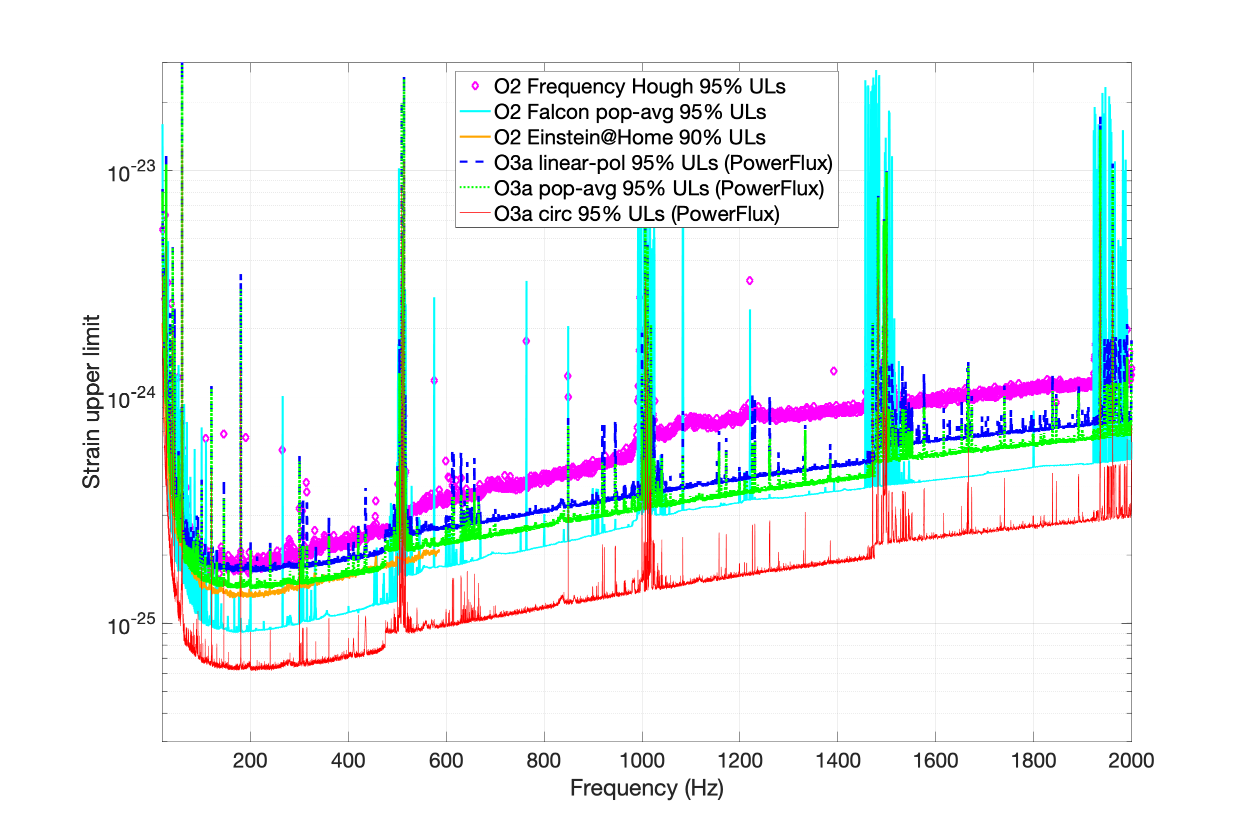
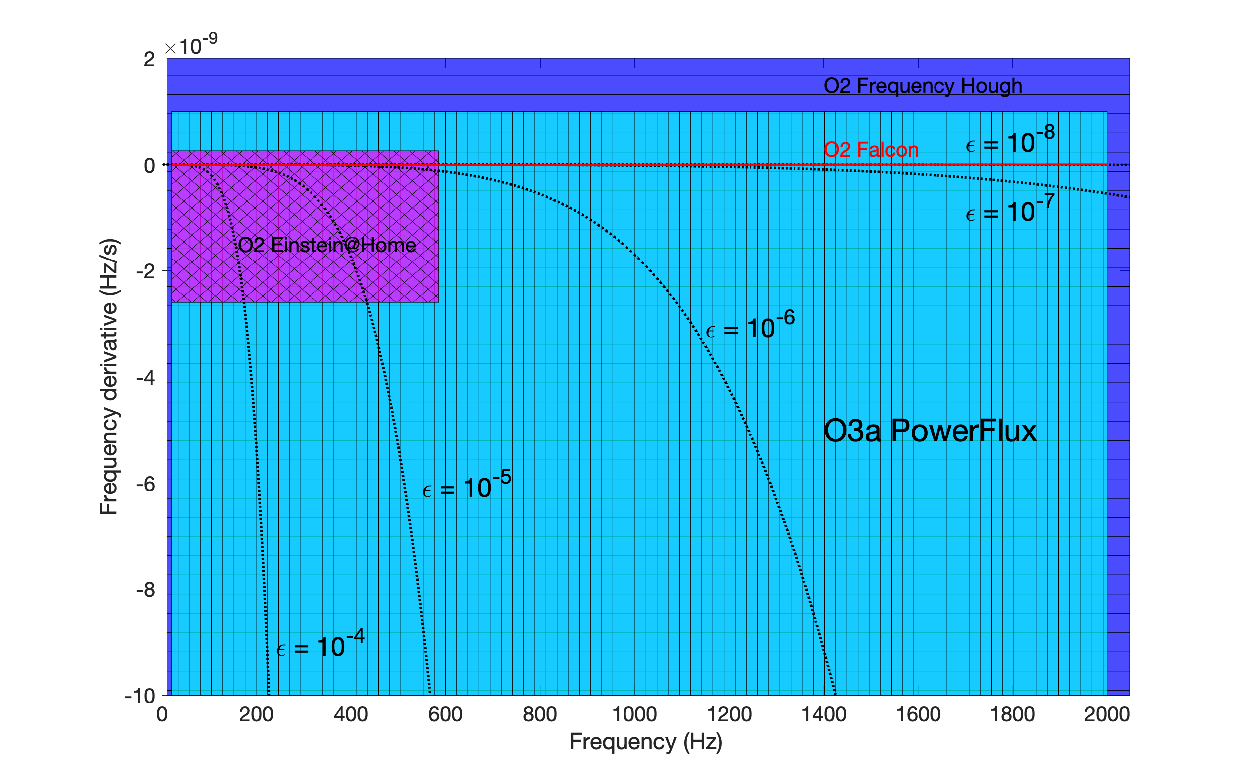
The most sensitive all-sky results to date for broad coverage of both frequency and spin-down were obtained recently from the full O3 data from three pipelines (Sky Hough, Frequency Hough and TD--statistic) (Abbott et al. 2022b) and are shown in Fig. 37, in comparison with the O3a PowerFlux results (Abbott et al. 2021a) and with the results from the new Viterbi-based, less sensitive but blazing-fast, SOAP pipeline. Also shown are recent O3a Falcon results (Dergachev and Papa 2022) over a restricted spin-down range. Figure 38 shows a comparison of the parameter space coverages of these different searches.
4.5 All-sky searches for binary stars
Several methods have been proposed and implemented for carrying out a CW all-sky binary search. The first method, which was used in a published search of initial LIGO S6 data (Aasi et al. 2014a) is known as TwoSpect (Goetz and Riles 2011). The program carries out a semi-coherent search over an observation time long compared to the maximum orbital period considered, while using coherence times short with respect to the orbital period. Fourier transforms are carried out over each row (fixed frequency bin) in a year-long spectrogram, and the resulting frequency-frequency plot is searched for characteristic harmonic patterns.
Another developed pipeline, known as Polynomial, (van der Putten et al. 2010) searches coherently using matched filters over an observation time short compared to the minimum orbital period considered. A bank of frequency polynomials in time is used for creating the matched filters, where for a small segment of an orbit, the frequency should vary as a low-order polynomial. Other proposed methods, which offer potentially substantial computational savings at a cost in sensitivity, include autocorrelations in the time-frequency plane (Viceré and Yvert 2016) and stochastic-background techniques (Ballmer 2006b), with computational costs gains achieved by using skymaps with sidereal-day folding (Thrane et al. 2015; Goncharov and Thrane 2018; Abbott et al. 2022a).
More recently, the implementation of graphics processor units software in the framework of the Sky Hough all-sky program has led to a breakthrough in all-sky binary search sensitivity (Covas and Sintes 2019). Upper limits were initially obtained over 100-300 Hz and over a broad range of binary orbital parameters from the LIGO O2 data (Covas and Sintes 2020). Although this approach does not yet cover the full orbital parameter space possible with the TwoSpect program, the intrinsic sensitivity is dramatically better, with extension of the method to shorter orbital periods a natural future improvement. A follow-up analysis in the O3a data (Abbott et al. 2021b; Tenorio 2021) expanded the search band slightly (50-300 Hz), and a parallel development using a similar Hough transform framework but with a -statistic (Covas and Prix 2022b; Covas and Prix 2022a) tailored to multi-hour segments, has been applied to the O3a data in the 300-500 Hz band (Covas et al. 2022). All of these results are shown in Figure 39. See references for details on orbital parameter space regions covered by the different analyses, which vary considerably.
In addition, searches for isolated stars retain some sensitivity to long-period binaries, as shown in a recent studies (Singh et al. 2019; Singh and Papa 2022).

4.6 Searches for CW transients and other CW-like signals
The first dedicated search for CW transients following a known pulsar’s glitch addressed glitches detected by radio astronomers during the Advanced LIGO / Virgo O2 data run. The search used the transient -statistic method (Prix et al. 2011) and focused on periods following glitches in the Crab and Vela pulsars (Keitel et al. 2019). A recent O3 analysis (Abbott et al. 2022f; Modafferi et al. 2021) searched for CW transients following nine glitches across six pulsars (one glitch each from five stars: PSR J0534+2200, J0908–4913, J1105–6107, J1813–1749 and J1826–1334; and four glitches from the intriguing source, PSR J0537-6910 – see sections 2.1.2, 2.1.4 and 4.2). No significant candidates were observed, although two marginal outliers were seen after one PSR J0537-6910 glitch, albeit with implied strengths well above those consistent with the inferred glitch energies. In fact, the upper limits obtained for post-glitch energy emission from all glitches examined lay above the maximum expected in a simple two-fluid model (Prix et al. 2011), with strain limits for PSR J1105-6107 approaching most closely to that benchmark (within a factor of 1.6).
The first dedicated search for long-lived, CW-like signals from a post-merger remnant looked for a signal from the post-GW170817 remnant, but as expected, given the 40 Mpc distance to the merger, no signal was detected in the immediate aftermath (Abbott et al. 2017o) (500 s) or in a multi-hour to multi-day period afterward (Abbott et al. 2019d). Should another opportunity arise (from a nearby binary neutron star merger or a galactic supernova), search methods are available for use (Thrane et al. 2011; Miller et al. 2018; Sun and Melatos 2019; Oliver et al. 2019; Banagiri et al. 2019; Mytidis et al. 2019; Miller et al. 2019a).
More exotic recent analyses seeking CW or CW-like signals include:
- •
Searches for CW signals from Bose-Einstein clouds (D’Antonio et al. 2018; Abbott et al. 2022c) (see section 2.2).
- •
A search for non-black-hole weakly interacting compact dark objects with mass below orbiting within the Sun about its center (Horowitz et al. 2020).
- •
Searches for ultralight dark photon or scalar boson dark matter creating an extremely narrowband () spectral excess with stochastic phase (Pierce et al. 2018; Guo et al. 2019; Miller et al. 2021b; Abbott et al. 2022d; Grote and Stadnik 2019; Vermeulen et al. 2021).
- •
A search for binary systems of planetary-scale / asteroid-scale primordial black holes near to the Earth (Miller et al. 2021a; Miller et al. 2022; Abbott et al. 2022b).
- •
There has also been a proposal to apply CW search techniques to suspected Thorne-Żytkow objects (Thorne and Zytkow 1975) (TZOs) for which a neutron star orbiting inside of a giant star (slow inspiral decay) could produce signals in the band of ground-based gravitational wave detectors (DeMarchi et al. 2021).
5 Outlook
5.1 Prospects for discovery
Over the next several years, the Advanced LIGO (Aasi et al. 2015a) and Virgo (Acernese et al. 2014) detectors are expected to approach and eventually surpass their original design sensitivities in strain, increasing the range within the galaxy which CW searches can access, thereby increasing detection likelihood. As the sensitive ranges of different search methods approach the dense galactic core, detection chances may rise more rapidly. In parallel to detector improvement, algorithms continue to improve, as researchers find more effective tradeoffs between computational cost and detection efficiency, while Moore’s Law, including Graphics Processing Unit (GPU) exploitation (Keitel and Ashton 2018; Covas and Sintes 2019; Wette et al. 2021; Dunn et al. 2021; La Rosa et al. 2021), ensures increased computing resources for searches. All of these trends are encouraging for successful CW detection.
At the same time, theoretical uncertainties in what sensitivity is needed for the first CW detection are very large. While the spin-down limits based on gravitar assumptions and on either energy conservation or known age have been beaten for a handful of sources and will be beaten for more sources in the coming years, the gravitar model is surely optimistic – most stellar spin-downs are likely dominated by electromagnetic interactions. Whether the first detection is imminent or still many years distant remains unclear. A recent phenomenological population synthesis study (Cieślar et al. 2021), based on an exponentially decaying ellipticity that starts at its allowed maximum with a supernova rate of once per century concluded that the expected number of detectable, young and isolated neutron stars for Advanced LIGO sensitivity is less than one and is 10 for Einstein Telescope.
Electromagnetic astronomers could prove pivotal in hastening detection by identifying new nearby or young neutron stars, or discovering pulsations from known stars, perhaps most usefully from the accreting Sco X-1 system (Galaudage et al. 2021). Given the computational challenges of most CW searches, narrowing the parameter space of a search exploiting electromagnetic observations could make the difference between a gravitational wave miss and a discovery.
5.2 Confirming and exploiting a discovery
There are several aspects of confirming a nominal CW discovery, including establishing the statistical significance of the outlier, verifying consistency of the signal with the CW model, excluding an environmental or instrumental cause, and (optionally but ideally) confirming consistency with prior or follow-up electromagnetic observations. Once that discovery is established, exploiting it to understand neutron star astrophysics (or fundamental particle physics should a superradiant boson cloud be observed) will be a rich endeavor.
The degree of statistical confidence with which a putative CW signal detection can be confirmed depends on the type of search that leads to the candidate. The statistical significance of an outlier depends on a trials factor that may range from 1 for targeted searches for known pulsars using electromagnetically derived ephemerides to for all-sky searches. Hence the SNR threshold for, say, a “5-sigma” discovery varies too. In practice, though, for a candidate emerging from a hierarchical search with multiple stages of “zooming in”, the SNR for a surviving outlier may be so much higher than the sensitivity-defining SNR threshold used in the first stage that the initial trials factor is irrelevant. Establishing the statistical confidence of a targeted-search candidate, on the other hand, may simply require steady accumulation of additional data while fully exploiting all data in hand from all detectors with appreciable sensitivity in that band. Empirically assessing the significance of loudest outliers is discussed in detail in (Tenorio et al. 2022).
If known detector artifacts are degrading sensitivity in the frequency band of the candidate, it may be feasible to focus detector commissioning to mitigate the artifact prior to the next observing run. Another possible approach, although potentially detrimental to other GW observations, is “narrowbanding.” In narrowbanding the detector sensitivity is improved in a narrow band at the expense of broadband sensitivity by adjusting the position of the “signal recycling” mirror at the output port of the interferometer (Aasi et al. 2015a); with the advent of quantum squeezing in advanced detectors (Tse et al. 2019), however, the potential gains from narrowbanding are less pronounced.
Even with a promising outlier, a discovery claim would need more than statistical inconsistency with detector noise. One would seek consistency with the signal model, particularly for candidates originating in hierarchical searches where early stages look primarily for excess power that is only roughly consistent with a particular template and where the spacing between templates is relatively coarse. The expected Doppler modulations due to the Earth’s motion should be present (Zhu et al. 2017; Intini et al. 2020b). One wants to see a signal for which a fully coherent search over all data yields an SNR consistent with expectation from the putative source. Ideally, a residual spectrum from subtracting the reconstructed signal would be consistent with random background noise.
In the case of a targeted or directed search for which the source location is a priori known, one would want to verify that the highest-SNR template observed in that region of the sky and near the template’s frequency parameters is indeed consistent with the correct sky location. Although one could impose a similar constraint on frequency and frequency derivatives for a targeted search, narrowband searches do allow those parameters to differ slightly from the nominal ones, to accommodate differential stellar rotation. Hence seeing the SNR peak at precisely the right location in parameter space for a known pulsar would lend credence to the signal, but seeing the SNR peak at a nearby point in parameter space can still mean discovery, albeit with a trials factor appropriate to a narrowband search.
The possibility of a rotational glitch during an observational period presents additional complications. One can no longer safely apply a fully coherent search over the time span and expect a monotonically increasing SNR. In the case of a targeted search with ephemerides in hand indicating a glitch, breaking the observation time into two (or more) segments is straightforward (Abbott et al. 2010), but in the case of a source without independent timing information, one may have a true signal detection but lack the confidence to declare discovery without additional data taking because of apparent phase inconsistency in the available data.
In any gravitational wave analysis using interferometers that push the frontier of technology (and which are routinely operated at maximum achievable sensitivity), one must consider whether or not instrumental or environmental contamination leads to a false signal. As discussed in section 3.7, narrow lines can contribute to accumulated power in a templated search. As part of confirming a discovery, one would need to quantify that contamination for a putative signal lying near a known instrumental spectral line. More challenging and more realistic for a signal candidate surviving multiple hierarchical search stages are spectral lines that are not immediately apparent in the strain channel spectrum, especially lines that are non-stationary with respect to time or frequency (“wandering”). To address that possibility, one would look comprehensively at auxiliary data channels, such as readouts from magnetometers, accelerometers, seismometers, microphones and from any servo control channels that could impose tiny actuations on the gravitational wave strain channel. Those investigations would include examination of averaged spectra for peaks coincident with the strain signal frequency and more probing searches for cross-coherence between the auxiliary channels and the strain channel that is inconsistent with statistical fluctuation.
The fact that the Virgo and KAGRA interferometers have made different technological choices means that instrumental contaminations differ, in general, from those of the LIGO interferometers, allowing better discrimination of astrophysical from instrumental sources. For example, a seemingly trivial but important difference is that the U.S. power mains used by LIGO, and the western Japanese power mains used by KAGRA provide alternating electrical currents at 60 Hz, but Virgo depends on Italian power mains which operate at 50 Hz. Since nearly all observatory electronics derive power from the mains, low-lying line contamination from the fundamental oscillation, from its higher harmonics and from sidebands due to non-linear interactions with mechanical and other electrical oscillations, are difficult to mitigate completely. Such technical differences reduce the chance of coincident false CW signals between the nominally identical LIGO detectors and the other two detectors.
Consistency in SNR detected by different interferometers offers another important astrophysical reality test. Unlike with transient GW detections, for which antenna pattern variations among detectors are critical to localization (Abbott et al. 2020b), any single interferometer can strongly localize a long-lived continous waves signal, largely removing antenna pattern / polarization ambiguity and permitting signal strength consistency comparisons across independent data sets in different interferometers (assuming the correctness of General Relativity GW polarization).
Finally, in confirming a continuous gravitational wave signal one would, ideally, want confirmation via electromagnetic observations. For targeted or narrowband searches of known pulsars, the observations already exist, and the primary task is to establish statistical confidence of their consistency with gravitational data. For other known sources, however, gravitational wave measurements may provide the necessary clues to allow detection of previously undetected pulsations. For example, detection of a CW signal from Scorpius X-1 could permit discrimination of X-ray pulsations from a stochastic background dominated by accretion emission. For a previously unknown source found in an all-sky search, determining the source location from coherent integration over months of data (with sub-arcsecond resolution possible from the aperture formed by the Earth’s orbit) may suffice for radio, X-ray, gamma-ray (and perhaps even optical) astronomers to find the counterpart. If electromagnetic pulsations were detected and agreed with expectation, the confirmation of the gravitational wave signal would be ironclad.
An interesting challenge to confirmation would be continuous gravitational radiation due to boson cloud superradiance for an isolated black hole (see section 2.2). If there were no accretion disk or companion to induce an electromagnetic signal, one would have to rely heavily upon the evolution of the gravitational wave signal itself to infer the nature of the source. In particular, the source frequency governed by the boson’s apparent mass in the potential of the black hole could spin up instead of down as the black hole loses mass energy to gravitational radiation, thereby reducing the magnitude of the negative binding energy correction to the unbound boson mass (Arvanitaki et al. 2015).
Once a continuous gravitational wave detection has been confirmed electromagnetically, one will want to exploit the correlations to understand the source. Below are a sampling of potential measurements possible, along with questions they help to address:
- •
Relation between rotational and gravitational wave frequencies, determining the fundamental mechanism of emission (see section 2 and see Jones 2021 for a detailed discussion).
- •
Correlation of the gravitational and electromagnetic phase constants in the event of consistent frequency (phase) evolution. If an equatorial mass “bulge” explains the GW signal, how well does the implied quadrupolar axis align with a pulsar’s inferred magnetic dipole projection? In an accreting system, for example, does added mass accumulate near the magnetic poles?
- •
Differential frequency (phase) evolution. Is there differential rotation between the stellar crust and its interior? If electromagnetic frequency glitches are observed, what is seen gravitationally before, during and after the glitch?
- •
If there is evidence for -modes from, say, an approximate 4/3 ratio of GW signal frequency to stellar rotation frequency, how does the GW frequency evolve with time and how does the ratio evolve? Is there evidence of amplitude growth from instability? Decay from viscosity?
- •
Inferred quadrupole moment. Although ellipticity is a convenient dimensionless parameter, it is approximately the product of the ellipticity times the stellar moment of inertia about its spin axis that determines the signal strength for a mass-quadrupole radiator. Given the uncertainties in neutron star equation of state, there are large uncertainties in the moment of inertia and hence ambiguity in extracting ellipticity. Ambiguity at the level of near-degeneracy would arise in the absence of an independent determination of source distance from electromagnetic observations (Sieniawska and Jones 2021). A CW detection in a binary system would offer an opportunity for determination of the stellar mass. Other stellar properties potentially accessible include the stellar radius (inferred from luminosity and temperature, if measurable). A precessing star with detectable electromagnetic pulsations offers additional opportunity for understanding internal structure (Gao et al. 2020).
- •
Even in the absence of detected electromagnetic pulsations, one can use the known source of an electromagnetic counterpart to infer a star’s moment of inertia, equatorial ellipticity, and the component of the magnetic dipole moment perpendicular to its rotation axis (Lu et al. 2022). For a close enough neutron star without an electromagnetic counterpart, parallax inference from the GW signal alone could resolve the degeneracy among source distance, moment of inertia and equatorial ellipticity (Sieniawska et al. 2022) (see Eqn. 14).
- •
Boson properties from superradiance. In the event of detecting superradiance from a boson cloud around a black hole, determining the boson’s mass will be immediate from the signal frequency (at least for the annihilation channel expected to dominate) with the boson intrinsic spin determination more model dependent, based on signal strength and frequency evolution with some knowledge of the black hole source needed.
In addition to exploiting CW detection to understand the source, one can also carry out precise tests of General Relativity by measuring the polarization of the propagating gravitational wave. In Einstein’s theory there should be two independent transverse, quadrupolar polarizations for which the relative strengths depend on the source orientation relative to the line of sight. In non-standard theories of gravity other polarization modes, including scalar, vector and longitudinal polarizations, may be present (Isi et al. 2015). Testing for these additional polarizations with transient gravitational wave detections to date has been challenging because nearly all of the signal-to-noise ratio has come from the two nearly aligned LIGO detectors such that they mainly detect the same polarization projection. In contrast, even for a single detector, a CW signal permits disentangling multiple polarization contributions as the sidereal rotation of the Earth changes the detector’s (polarimeter’s) orientation with respect to the source direction deterministically (Isi et al. 2015; Kuwahara and Asada 2022). In fact, even in the absence of a CW signal, one can set upper limits on the non-standard polarizations (Abbott et al. 2018a), just as is possible for standard polarizations.
Nature has blessed the gravitational wave community with a bounty of compact star mergers, including the remarkable first detected BBH merger, GW150914, and the even more remarkable and informative multi-messenger detection of the GW170817 BNS event. Should such kindness continue, one may hope soon for a multi-messenger detection of a CW source that not only could be observed into the foreseeable future, but could mark the first of a large collection to come, as GW150914 proved to be.
Acknowledgements.
The author is deeply grateful to current and former colleagues in the LIGO Scientific Collaboration and Virgo collaboration Continuous Waves Search Group for close collaboration from which he has benefited in preparing this article. The author also thanks Julian Carlin, Pep Covas, Vladimir Dergachev, Francesco Fidecaro, Bryn Haskell, Wynn Ho, Ian Jones, David Keitel, Andrew Melatos, Ben Owen, Maria Alessandra Papa, Lilli Sun, Rodrigo Tenorio, Karl Wette and Graham Woan for helpful suggestions concerning the manuscript. Special thanks to the two anonymous referees for their thorough readings and for many constructive suggestions (and corrections). Thanks too to LIGO, Virgo and the Max Planck Institute f. Gravitational Physics for the use of figures. This work was supported in part by National Science Foundation Awards PHY-1505932 and PHY-1806577. The author thanks the Institute of Nuclear Theory at the University of Washington and the Perimeter Institute of Waterloo for hosting workshops that proved helpful in composing this review. The author is grateful for computational resources provided by the LIGO Laboratory and is supported by the National Science Foundation. This material is based in part upon work supported by NSF’s LIGO Laboratory which is a major facility fully funded by the National Science Foundation.References
- Aasi et al. (2013a) Aasi J, et al. (2013a) Directed search for continuous gravitational waves from the Galactic center. Physical Review D 88(10), DOI: 10.1103/physrevd.88.102002
- Aasi et al. (2013b) Aasi J, et al. (2013b) Einstein@Home all-sky search for periodic gravitational waves in LIGO S5 data. Phys Rev D 87(4):042001, DOI: 10.1103/PhysRevD.87.042001, arXiv: 1207.7176
- Aasi et al. (2014a) Aasi J, et al. (2014a) First all-sky search for continuous gravitational waves from unknown sources in binary systems. Phys Rev D 90(6):062010, DOI: 10.1103/PhysRevD.90.062010, arXiv: 1405.7904
- Aasi et al. (2014b) Aasi J, et al. (2014b) Gravitational Waves from Known Pulsars: Results from the Initial Detector Era. The Astrophysical Journal 785(2):119, DOI: 10.1088/0004-637x/785/2/119
- Aasi et al. (2014c) Aasi J, et al. (2014c) Implementation of an -statistic all-sky search for continuous gravitational waves in Virgo VSR1 data. Classical and Quantum Gravity 31(16):165014, DOI: 10.1088/0264-9381/31/16/165014
- Aasi et al. (2015a) Aasi J, et al. (2015a) Advanced LIGO. Classical and Quantum Gravity 32(7):074001, DOI: 10.1088/0264-9381/32/7/074001
- Aasi et al. (2015b) Aasi J, et al. (2015b) Characterization of the LIGO detectors during their sixth science run. Classical and Quantum Gravity 32(11):115012, DOI: 10.1088/0264-9381/32/11/115012
- Aasi et al. (2015c) Aasi J, et al. (2015c) Directed search for gravitational waves from Scorpius X-1 with initial LIGO data. Phys Rev D 91:062008, DOI: 10.1103/PhysRevD.91.062008
- Aasi et al. (2015d) Aasi J, et al. (2015d) Narrow-band search of continuous gravitational-wave signals from Crab and Vela pulsars in Virgo VSR4 data. Physical Review D 91(2), DOI: 10.1103/physrevd.91.022004
- Aasi et al. (2015e) Aasi J, et al. (2015e) Searches for continuous gravitational waves from nine young supernova remnants. The Astrophysical Journal 813(1):39, DOI: 10.1088/0004-637x/813/1/39
- Aasi et al. (2016a) Aasi J, et al. (2016a) First low frequency all-sky search for continuous gravitational wave signals. Phys Rev D 93:042007, DOI: 10.1103/PhysRevD.93.042007
- Aasi et al. (2016b) Aasi J, et al. (2016b) Search of the Orion spur for continuous gravitational waves using a loosely coherent algorithm on data from LIGO interferometers. Phys Rev D 93:042006, DOI: 10.1103/PhysRevD.93.042006
- Abadie et al. (2010) Abadie J, et al. (2010) First search for gravitational waves from the youngest known neutron star. The Astrophysical Journal 722(2):1504–1513, DOI: 10.1088/0004-637x/722/2/1504
- Abadie et al. (2011) Abadie J, et al. (2011) Beating the Spin-down Limit on Gravitational Wave Emission from the Vela pulsar. The Astrophysical Journal 737(2):93, DOI: 10.1088/0004-637x/737/2/93
- Abadie et al. (2012) Abadie J, et al. (2012) All-sky search for periodic gravitational waves in the full S5 LIGO data. Physical Review D 85(2):022001, DOI: 10.1103/physrevd.85.022001
- Abazajian (2011) Abazajian KN (2011) The Consistency of Fermi-LAT Observations of the Galactic Center with a Millisecond Pulsar Population in the Central Stellar Cluster. JCAP 03:010, DOI: 10.1088/1475-7516/2011/03/010, arXiv: 1011.4275
- Abbott et al. (2004) Abbott BP, et al. (2004) Setting upper limits on the strength of periodic gravitational waves from PSR using the first science data from the GEO 600 and LIGO detectors. Phys Rev D 69:082004, DOI: 10.1103/PhysRevD.69.082004
- Abbott et al. (2005a) Abbott BP, et al. (2005a) First all-sky upper limits from LIGO on the strength of periodic gravitational waves using the Hough transform. Phys Rev D 72:102004, DOI: 10.1103/PhysRevD.72.102004, arXiv: gr-qc/0508065
- Abbott et al. (2005b) Abbott BP, et al. (2005b) Limits on Gravitational-Wave Emission from Selected Pulsars Using LIGO Data. Phys Rev Lett 94:181103, DOI: 10.1103/PhysRevLett.94.181103
- Abbott et al. (2007a) Abbott BP, et al. (2007a) Searches for periodic gravitational waves from unknown isolated sources and Scorpius X-1: Results from the second LIGO science run. Phys Rev D 76:082001, DOI: 10.1103/PhysRevD.76.082001
- Abbott et al. (2007b) Abbott BP, et al. (2007b) Upper limits on gravitational wave emission from 78 radio pulsars. Phys Rev D 76:042001, DOI: 10.1103/PhysRevD.76.042001
- Abbott et al. (2008a) Abbott BP, et al. (2008a) All-sky search for periodic gravitational waves in LIGO S4 data. Phys Rev D 77:022001, DOI: 10.1103/PhysRevD.77.022001, [Erratum: Phys.Rev.D 80, 129904 (2009)], arXiv: 0708.3818
- Abbott et al. (2008b) Abbott BP, et al. (2008b) Beating the Spin-Down Limit on Gravitational Wave Emission from the Crab Pulsar. Astrophys J Lett 683(1):L45, DOI: 10.1086/591526, arXiv: 0805.4758
- Abbott et al. (2009a) Abbott BP, et al. (2009a) All-sky LIGO Search for Periodic Gravitational Waves in the Early S5 Data. Phys Rev Lett 102:111102, DOI: 10.1103/PhysRevLett.102.111102, arXiv: 0810.0283
- Abbott et al. (2009b) Abbott BP, et al. (2009b) Einstein@Home search for periodic gravitational waves in early S5 LIGO data. Phys Rev D 80:042003, DOI: 10.1103/PhysRevD.80.042003, arXiv: 0905.1705
- Abbott et al. (2009c) Abbott BP, et al. (2009c) The Einstein@Home search for periodic gravitational waves in LIGO S4 data. Phys Rev D 79:022001, DOI: 10.1103/PhysRevD.79.022001, arXiv: 0804.1747
- Abbott et al. (2010) Abbott BP, et al. (2010) Searches for Gravitational Waves from Known Pulsars with Science Run 5 LIGO Data. The Astrophysical Journal 713(1):671–685, DOI: 10.1088/0004-637x/713/1/671
- Abbott et al. (2016a) Abbott BP, et al. (2016a) Comprehensive all-sky search for periodic gravitational waves in the sixth science run LIGO data. Phys Rev D 94(4):042002, DOI: 10.1103/PhysRevD.94.042002, arXiv: 1605.03233
- Abbott et al. (2016b) Abbott BP, et al. (2016b) GW150914: The Advanced LIGO Detectors in the Era of First Discoveries. Phys Rev Lett 116(13):131103, DOI: 10.1103/PhysRevLett.116.131103, arXiv: 1602.03838
- Abbott et al. (2016c) Abbott BP, et al. (2016c) GW150914: The Advanced LIGO Detectors in the Era of First Discoveries. Phys Rev Lett 116:131103, DOI: 10.1103/PhysRevLett.116.131103
- Abbott et al. (2016d) Abbott BP, et al. (2016d) GW151226: Observation of Gravitational Waves from a 22-Solar-Mass Binary Black Hole Coalescence. Phys Rev Lett 116:241103, DOI: 10.1103/PhysRevLett.116.241103
- Abbott et al. (2016e) Abbott BP, et al. (2016e) Results of the deepest all-sky survey for continuous gravitational waves on LIGO S6 data running on the Einstein@Home volunteer distributed computing project. Phys Rev D 94(10):102002, DOI: 10.1103/PhysRevD.94.102002, arXiv: 1606.09619
- Abbott et al. (2017a) Abbott BP, et al. (2017a) All-sky Search for Periodic Gravitational Waves in the O1 LIGO Data. Phys Rev D 96(6):062002, DOI: 10.1103/PhysRevD.96.062002, arXiv: 1707.02667
- Abbott et al. (2017b) Abbott BP, et al. (2017b) Directional Limits on Persistent Gravitational Waves from Advanced LIGO’s First Observing Run. Phys Rev Lett 118:121102, DOI: 10.1103/PhysRevLett.118.121102
- Abbott et al. (2017c) Abbott BP, et al. (2017c) Exploring the sensitivity of next generation gravitational wave detectors. Classical and Quantum Gravity 34(4):044001, DOI: 10.1088/1361-6382/aa51f4
- Abbott et al. (2017d) Abbott BP, et al. (2017d) First low-frequency Einstein@Home all-sky search for continuous gravitational waves in Advanced LIGO data. Phys Rev D 96(12):122004, DOI: 10.1103/PhysRevD.96.122004, arXiv: 1707.02669
- Abbott et al. (2017e) Abbott BP, et al. (2017e) First narrow-band search for continuous gravitational waves from known pulsars in advanced detector data. Phys Rev D 96:122006, DOI: 10.1103/PhysRevD.96.122006
- Abbott et al. (2017f) Abbott BP, et al. (2017f) First search for gravitational waves from known pulsars with Advanced LIGO. Astrophys J 839(1):12, DOI: 10.3847/1538-4357/aa677f, [Erratum: Astrophys.J. 851, 71 (2017)], arXiv: 1701.07709
- Abbott et al. (2017g) Abbott BP, et al. (2017g) Gravitational Waves and Gamma-Rays from a Binary Neutron Star Merger: GW170817 and GRB 170817A. The Astrophysical Journal 848(2):L13, DOI: 10.3847/2041-8213/aa920c
- Abbott et al. (2017h) Abbott BP, et al. (2017h) GW170104: Observation of a 50-Solar-Mass Binary Black Hole Coalescence at Redshift 0.2. Phys Rev Lett 118:221101, DOI: 10.1103/PhysRevLett.118.221101
- Abbott et al. (2017i) Abbott BP, et al. (2017i) GW170608: Observation of a 19-solar-mass Binary Black Hole Coalescence. Astrophys J 851(2):L35, DOI: 10.3847/2041-8213/aa9f0c, arXiv: 1711.05578
- Abbott et al. (2017j) Abbott BP, et al. (2017j) GW170814: A Three-Detector Observation of Gravitational Waves from a Binary Black Hole Coalescence. Phys Rev Lett 119:141101, DOI: 10.1103/PhysRevLett.119.141101
- Abbott et al. (2017k) Abbott BP, et al. (2017k) GW170817: Observation of Gravitational Waves from a Binary Neutron Star Inspiral. Phys Rev Lett 119:161101, DOI: 10.1103/PhysRevLett.119.161101
- Abbott et al. (2017l) Abbott BP, et al. (2017l) Multi-messenger Observations of a Binary Neutron Star Merger. Astrophys J Lett 848(2):L12, DOI: 10.3847/2041-8213/aa91c9, arXiv: 1710.05833
- Abbott et al. (2017m) Abbott BP, et al. (2017m) Search for continuous gravitational waves from neutron stars in globular cluster NGC 6544. Phys Rev D 95:082005, DOI: 10.1103/PhysRevD.95.082005
- Abbott et al. (2017n) Abbott BP, et al. (2017n) Search for gravitational waves from Scorpius X-1 in the first Advanced LIGO observing run with a hidden Markov model. Phys Rev D 95:122003, DOI: 10.1103/PhysRevD.95.122003
- Abbott et al. (2017o) Abbott BP, et al. (2017o) Search for Post-merger Gravitational Waves from the Remnant of the Binary Neutron Star Merger GW170817. Astrophys J Lett 851(1):L16, DOI: 10.3847/2041-8213/aa9a35, arXiv: 1710.09320
- Abbott et al. (2017p) Abbott BP, et al. (2017p) Upper Limits on Gravitational Waves from Scorpius X-1 from a Model-based Cross-correlation Search in Advanced LIGO Data. The Astrophysical Journal 847(1):47, DOI: 10.3847/1538-4357/aa86f0
- Abbott et al. (2018a) Abbott BP, et al. (2018a) First search for nontensorial gravitational waves from known pulsars. Phys Rev Lett 120(3):031104, DOI: 10.1103/PhysRevLett.120.031104, arXiv: 1709.09203
- Abbott et al. (2018b) Abbott BP, et al. (2018b) Full Band All-sky Search for Periodic Gravitational Waves in the O1 LIGO Data. Phys Rev D 97(10):102003, DOI: 10.1103/PhysRevD.97.102003, arXiv: 1802.05241
- Abbott et al. (2018c) Abbott BP, et al. (2018c) GW170817: Measurements of Neutron Star Radii and Equation of State. Phys Rev Lett 121:161101, DOI: 10.1103/PhysRevLett.121.161101
- Abbott et al. (2019a) Abbott BP, et al. (2019a) All-sky search for continuous gravitational waves from isolated neutron stars using Advanced LIGO O2 data. Phys Rev D 100(2):024004, DOI: 10.1103/PhysRevD.100.024004, arXiv: 1903.01901
- Abbott et al. (2019b) Abbott BP, et al. (2019b) GWTC-1: A Gravitational-Wave Transient Catalog of Compact Binary Mergers Observed by LIGO and Virgo during the First and Second Observing Runs. Phys Rev X 9:031040, DOI: 10.1103/PhysRevX.9.031040
- Abbott et al. (2019c) Abbott BP, et al. (2019c) Narrow-band search for gravitational waves from known pulsars using the second LIGO observing run. Physical Review D 99(12), DOI: 10.1103/physrevd.99.122002
- Abbott et al. (2019d) Abbott BP, et al. (2019d) Search for gravitational waves from a long-lived remnant of the binary neutron star merger GW170817. Astrophys J 875(2):160, DOI: 10.3847/1538-4357/ab0f3d, arXiv: 1810.02581
- Abbott et al. (2019e) Abbott BP, et al. (2019e) Search for gravitational waves from Scorpius X-1 in the second Advanced LIGO observing run with an improved hidden Markov model. Physical Review D 100(12), DOI: 10.1103/physrevd.100.122002
- Abbott et al. (2019a) Abbott BP, et al. (2019a) Searches for Continuous Gravitational Waves from 15 Supernova Remnants and Fomalhaut b with Advanced LIGO. The Astrophysical Journal 875(2):122, DOI: 10.3847/1538-4357/ab113b, arXiv: 1812.11656
- Abbott et al. (2019b) Abbott BP, et al. (2019b) Searches for Gravitational Waves from Known Pulsars at Two Harmonics in 2015-2017 LIGO Data. The Astrophysical Journal 879(1):10, DOI: 10.3847/1538-4357/ab20cb, arXiv: 1902.08507
- Abbott et al. (2020a) Abbott BP, et al. (2020a) GW190425: Observation of a Compact Binary Coalescence with Total Mass . Astrophys J Lett 892(1):L3, DOI: 10.3847/2041-8213/ab75f5, arXiv: 2001.01761
- Abbott et al. (2020b) Abbott BP, et al. (2020b) Prospects for observing and localizing gravitational-wave transients with advanced ligo, advanced virgo and kagra. Living Reviews in Relativity 23(1):3, DOI: 10.1007/s41114-020-00026-9
- Abbott et al. (2020c) Abbott R, et al. (2020c) Gravitational-wave Constraints on the Equatorial Ellipticity of Millisecond Pulsars. The Astrophysical Journal Letters 902(1):L21, DOI: 10.3847/2041-8213/abb655
- Abbott et al. (2020d) Abbott R, et al. (2020d) GW190521: A Binary Black Hole Merger with a Total Mass of . Phys Rev Lett 125(10):101102, DOI: 10.1103/PhysRevLett.125.101102, arXiv: 2009.01075
- Abbott et al. (2020e) Abbott R, et al. (2020e) GW190814: Gravitational Waves from the Coalescence of a 23 Solar Mass Black Hole with a 2.6 Solar Mass Compact Object. The Astrophysical Journal 896(2):L44, DOI: 10.3847/2041-8213/ab960f
- Abbott et al. (2021a) Abbott R, et al. (2021a) All-sky search for continuous gravitational waves from isolated neutron stars in the early O3 LIGO data. Physical Review D 104(8), DOI: 10.1103/physrevd.104.082004
- Abbott et al. (2021b) Abbott R, et al. (2021b) All-sky search in early O3 LIGO data for continuous gravitational-wave signals from unknown neutron stars in binary systems. Phys Rev D 103:064017, DOI: 10.1103/PhysRevD.103.064017
- Abbott et al. (2021c) Abbott R, et al. (2021c) Constraints from LIGO O3 Data on Gravitational-wave Emission Due to R-modes in the Glitching Pulsar PSR J0537–6910. The Astrophysical Journal 922(1):71, DOI: 10.3847/1538-4357/ac0d52
- Abbott et al. (2021d) Abbott R, et al. (2021d) Diving below the Spin-down Limit: Constraints on Gravitational Waves from the Energetic Young Pulsar PSR J0537-6910. The Astrophysical Journal Letters 913(2):L27, DOI: 10.3847/2041-8213/abffcd
- Abbott et al. (2021e) Abbott R, et al. (2021e) GWTC-2: Compact Binary Coalescences Observed by LIGO and Virgo during the First Half of the Third Observing Run. Phys Rev X 11:021053, DOI: 10.1103/PhysRevX.11.021053
- Abbott et al. (2021f) Abbott R, et al. (2021f) GWTC-3: Compact Binary Coalescences Observed by LIGO and Virgo During the Second Part of the Third Observing Run. arXiv: 2111.03606
- Abbott et al. (2021g) Abbott R, et al. (2021g) Observation of Gravitational Waves from Two Neutron Star–Black Hole Coalescences. Astrophys J Lett 915(1):L5, DOI: 10.3847/2041-8213/ac082e, arXiv: 2106.15163
- Abbott et al. (2021h) Abbott R, et al. (2021h) Search for anisotropic gravitational-wave backgrounds using data from Advanced LIGO and Advanced Virgo’s first three observing runs. Phys Rev D 104(2):022005, DOI: 10.1103/PhysRevD.104.022005, arXiv: 2103.08520
- Abbott et al. (2021i) Abbott R, et al. (2021i) Searches for Continuous Gravitational Waves from Young Supernova Remnants in the Early Third Observing Run of Advanced LIGO and Virgo. The Astrophysical Journal 921(1):80, DOI: 10.3847/1538-4357/ac17ea
- Abbott et al. (2022a) Abbott R, et al. (2022a) All-sky, all-frequency directional search for persistent gravitational waves from advanced ligo’s and advanced virgo’s first three observing runs. Phys Rev D 105:122001, DOI: 10.1103/PhysRevD.105.122001, arXiv: 2110.09834
- Abbott et al. (2022b) Abbott R, et al. (2022b) All-sky search for continuous gravitational waves from isolated neutron stars using advanced ligo and advanced virgo o3 data. Phys Rev D 106:102008, DOI: 10.1103/PhysRevD.106.102008, arXiv: 2201.00697
- Abbott et al. (2022c) Abbott R, et al. (2022c) All-sky search for gravitational wave emission from scalar boson clouds around spinning black holes in LIGO O3 data. Phys Rev D 105:102001, DOI: 10.1103/PhysRevD.105.102001, arXiv: 2111.15507
- Abbott et al. (2022d) Abbott R, et al. (2022d) Constraints on dark photon dark matter using data from LIGO’s and Virgo’s third observing run. Phys Rev D 105:063030, DOI: 10.1103/PhysRevD.105.063030, arXiv: 2105.13085
- Abbott et al. (2022e) Abbott R, et al. (2022e) Model-based Cross-correlation Search for Gravitational Waves from the Low-mass X-Ray Binary Scorpius X-1 in LIGO O3 Data. The Astrophysical Journal Letters 941(2):L30, DOI: 10.3847/2041-8213/aca1b0, arXiv: 2209.02863
- Abbott et al. (2022f) Abbott R, et al. (2022f) Narrowband searches for continuous and long-duration transient gravitational waves from known pulsars in the ligo-virgo third observing run. The Astrophysical Journal 932(2):133, DOI: 10.3847/1538-4357/ac6ad0, URL https://dx.doi.org/10.3847/1538-4357/ac6ad0, arXiv: 2112.10990
- Abbott et al. (2022g) Abbott R, et al. (2022g) Search for continuous gravitational waves from 20 accreting millisecond x-ray pulsars in O3 LIGO data. Phys Rev D 105:022002, DOI: 10.1103/PhysRevD.105.022002
- Abbott et al. (2022h) Abbott R, et al. (2022h) Search for gravitational waves from Scorpius X-1 with a hidden Markov model in O3 LIGO data. Phys Rev D 106(6):062002, DOI: 10.1103/PhysRevD.106.062002, arXiv: 2201.10104
- Abbott et al. (2022i) Abbott R, et al. (2022i) Search of the Early O3 LIGO Data for Continuous Gravitational Waves from the Cassiopeia A and Vela Jr. Supernova Remnants. Phys Rev D 105:082005, DOI: 10.1103/PhysRevD.105.082005, arXiv: 2111.15116
- Abbott et al. (2022j) Abbott R, et al. (2022j) Searches for gravitational waves from known pulsars at two harmonics in the second and third ligo-virgo observing runs. The Astrophysical Journal 935(1):1, DOI: 10.3847/1538-4357/ac6acf, URL https://dx.doi.org/10.3847/1538-4357/ac6acf, arXiv: 2111.13106
- Acernese et al. (2014) Acernese F, et al. (2014) Advanced Virgo: a second-generation interferometric gravitational wave detector. Classical and Quantum Gravity 32(2):024001, DOI: 10.1088/0264-9381/32/2/024001
- Ackermann et al. (2017) Ackermann M, et al. (2017) The Fermi Galactic Center GeV Excess and Implications for Dark Matter. Astrophys J 840(1):43, DOI: 10.3847/1538-4357/aa6cab, arXiv: 1704.03910
- Aharonian et al. (2005) Aharonian F, et al. (2005) A New Population of Very High Energy Gamma-Ray Sources in the Milky Way. Science 307(5717):1938–1942, DOI: 10.1126/science.1108643, arXiv: astro-ph/0504380
- Aharonian et al. (2008) Aharonian F, et al. (2008) HESS very-high-energy gamma-ray sources without identified counterparts. Astron Astrophys 477(1):353–363, DOI: 10.1051/0004-6361:20078516, arXiv: 0712.1173
- Alarie et al. (2014) Alarie A, Bilodeau A, Drissen L (2014) A hyperspectral view of Cassiopeia A. Monthly Notices of the Royal Astronomical Society 441:2996–3008
- Alford and Schwenzer (2014) Alford MG, Schwenzer K (2014) Gravitational wave emission and spindown of young pulsars. Astrophys J 781:26, DOI: 10.1088/0004-637X/781/1/26, arXiv: 1210.6091
- Alford and Schwenzer (2015) Alford MG, Schwenzer K (2015) Gravitational wave emission from oscillating millisecond pulsars. Mon Not Roy Astron Soc 446(4):3631–3641, DOI: 10.1093/mnras/stu2361, arXiv: 1403.7500
- Allen (2019) Allen B (2019) Spherical ansatz for parameter-space metrics. Phys Rev D 100(12):124004, DOI: 10.1103/PhysRevD.100.124004, arXiv: 1906.01352
- Allen (2021) Allen B (2021) Optimal template banks. Phys Rev D 104(4):042005, DOI: 10.1103/PhysRevD.104.042005, arXiv: 2102.11254
- Allen et al. (1999) Allen B, Hua W, Ottewill A (1999) Automatic cross-talk removal from multi-channel data. arXiv: gr-qc/9909083
- Allen et al. (2002) Allen B, Papa MA, Schutz BF (2002) Optimal strategies for sinusoidal signal detection. Phys Rev D 66:102003, DOI: 10.1103/PhysRevD.66.102003
- Allen et al. (2015) Allen GE, Chow K, DeLaney T, Filipovic MD, Houck JC, Pannuti TG, Stage MD (2015) On the Expansion Rate, Age, and Distance of the Supernova Remnant G266.2-1.2 (Vela Jr.). Astrophys J 798(2):82, DOI: 10.1088/0004-637X/798/2/82, arXiv: 1410.7435
- Alpar et al. (1982) Alpar MA, Cheng AF, Ruderman MA, Shaham J (1982) A new class of radio pulsars. Nature 300(5894):728–730, DOI: 10.1038/300728a0
- Althouse et al. (1998) Althouse B, Jones L, Lazzarini A (1998) Determination of Global and Local Coordinate Axes for the LIGO Sites. LIGO Report T980044, URL https://dcc.ligo.org/T980044
- Anderson et al. (2002) Anderson DP, Cobb J, Korpela E, Lebofsky M, Werthimer D (2002) SETI@home: An Experiment in Public-Resource Computing. Commun ACM 45(11):56–61, DOI: 10.1145/581571.581573
- Andersson (1998) Andersson N (1998) A New class of unstable modes of rotating relativistic stars. Astrophys J 502:708–713, DOI: 10.1086/305919, arXiv: gr-qc/9706075
- Andersson (2019) Andersson N (2019) Gravitational-Wave Astronomy: Exploring the Dark Side of the Universe. Oxford University Press, DOI: 10.1093/oso/9780198568032.001.0001
- Andersson et al. (2014) Andersson N, Jones DI, Ho WCG (2014) Implications of an r-mode in XTE J1751-305: Mass, radius and spin evolution. Mon Not Roy Astron Soc 442(2):1786–1793, DOI: 10.1093/mnras/stu870, arXiv: 1403.0860
- Andersson et al. (2018) Andersson N, Antonopoulou D, Espinoza C, Haskell B, Ho W (2018) The Enigmatic Spin Evolution of PSR J0537–6910: r-modes, Gravitational Waves, and the Case for Continued Timing. Astrophys J 864(2):137, DOI: 10.3847/1538-4357/aad6eb, arXiv: 1711.05550
- Antoniadis et al. (2013) Antoniadis J, Freire PCC, Wex N, Tauris TM, Lynch RS, van Kerkwijk MH, Kramer M, Bassa C, Dhillon VS, Driebe T, Hessels JWT, Kaspi VM, Kondratiev VI, Langer N, Marsh TR, McLaughlin MA, Pennucci TT, Ransom SM, Stairs IH, van Leeuwen J, Verbiest JPW, Whelan DG (2013) A Massive Pulsar in a Compact Relativistic Binary. Science 340(6131):448, DOI: 10.1126/science.1233232, arXiv: 1304.6875
- Antonopoulou et al. (2018) Antonopoulou D, Espinoza CM, Kuiper L, Andersson N (2018) Pulsar spin-down: the glitch-dominated rotation of PSR J05376910. Mon Not Roy Astron Soc 473(2):1644–1655, DOI: 10.1093/mnras/stx2429, arXiv: 1708.09459
- Antonucci et al. (2008) Antonucci F, Astone P, D’Antonio S, Frasca S, Palomba C (2008) Detection of periodic gravitational wave sources by Hough transform in the f versus \skew6\dot f plane. Classical and Quantum Gravity 25(18):184015, DOI: 10.1088/0264-9381/25/18/184015
- de Araujo et al. (2016) de Araujo JCN, Coelho JG, Costa CA (2016) Gravitational Waves from Pulsars and their Braking Indices: The Role of a Time Dependent Magnetic Ellipticity. The Astrophysical Journal 831(1):35, DOI: 10.3847/0004-637x/831/1/35
- de Araujo et al. (2017) de Araujo JCN, Coelho JG, Costa CA (2017) Gravitational waves from pulsars in the context of magnetic ellipticity. The European Physical Journal C 77(5), DOI: 10.1140/epjc/s10052-017-4925-3
- Archibald et al. (2009) Archibald AM, Stairs IH, Ransom SM, Kaspi VM, Kondratiev VI, Lorimer DR, McLaughlin MA, Boyles J, Hessels JWT, Lynch R, van Leeuwen J, Roberts MSE, Jenet F, Champion DJ, Rosen R, Barlow BN, Dunlap BH, Remillard RA (2009) A Radio Pulsar/X-ray Binary Link. Science 324(5933):1411–1414, DOI: 10.1126/science.1172740
- Archibald et al. (2016) Archibald RF, Gotthelf EV, Ferdman RD, Kaspi VM, Guillot S, Harrison FA, Keane EF, Pivovaroff MJ, Stern D, Tendulkar SP, et al (2016) A High Braking Index for a Pulsar. The Astrophysical Journal 819(1):L16, DOI: 10.3847/2041-8205/819/1/l16
- Arras et al. (2003) Arras P, Flanagan EE, Morsink SM, Schenk A, Teukolsky SA, Wasserman I (2003) Saturation of the R mode instability. Astrophys J 591:1129–1151, DOI: 10.1086/374657, arXiv: astro-ph/0202345
- Arvanitaki and Dubovsky (2011) Arvanitaki A, Dubovsky S (2011) Exploring the String Axiverse with Precision Black Hole Physics. Phys Rev D 83:044026, DOI: 10.1103/PhysRevD.83.044026, arXiv: 1004.3558
- Arvanitaki et al. (2010) Arvanitaki A, Dimopoulos S, Dubovsky S, Kaloper N, March-Russell J (2010) String axiverse. Phys Rev D 81:123530, DOI: 10.1103/PhysRevD.81.123530
- Arvanitaki et al. (2015) Arvanitaki A, Baryakhtar M, Huang X (2015) Discovering the QCD Axion with Black Holes and Gravitational Waves. Phys Rev D 91(8):084011, DOI: 10.1103/PhysRevD.91.084011, arXiv: 1411.2263
- Arvanitaki et al. (2017) Arvanitaki A, Baryakhtar M, Dimopoulos S, Dubovsky S, Lasenby R (2017) Black hole mergers and the QCD axion at Advanced LIGO. Phys Rev D 95:043001, DOI: 10.1103/PhysRevD.95.043001
- Arzoumanian et al. (2018) Arzoumanian Z, Brazier A, Burke-Spolaor S, Chamberlin S, Chatterjee S, Christy B, Cordes JM, Cornish NJ, Crawford F, Thankful Cromartie H, Crowter K, DeCesar ME, Demorest PB, Dolch T, Ellis JA, Ferdman RD, Ferrara EC, Fonseca E, Garver-Daniels N, Gentile PA, Halmrast D, Huerta EA, Jenet FA, Jessup C, Jones G, Jones ML, Kaplan DL, Lam MT, Lazio TJW, Levin L, Lommen A, Lorimer DR, Luo J, Lynch RS, Madison D, Matthews AM, McLaughlin MA, McWilliams ST, Mingarelli C, Ng C, Nice DJ, Pennucci TT, Ransom SM, Ray PS, Siemens X, Simon J, Spiewak R, Stairs IH, Stinebring DR, Stovall K, Swiggum JK, Taylor SR, Vallisneri M, van Haasteren R, Vigeland SJ, Zhu W, NANOGrav Collaboration (2018) The NANOGrav 11-year Data Set: High-precision Timing of 45 Millisecond Pulsars. Astrophys J Suppl 235(2):37, DOI: 10.3847/1538-4365/aab5b0, arXiv: 1801.01837
- Ashok et al. (2021) Ashok A, Beheshtipour B, Papa MA, Freire PCC, Steltner B, Machenschalk B, Behnke O, Allen B, Prix R (2021) New Searches for Continuous Gravitational Waves from Seven Fast Pulsars. The Astrophysical Journal 923(1):85, DOI: 10.3847/1538-4357/ac2582
- Ashton and Prix (2018) Ashton G, Prix R (2018) Hierarchical multistage MCMC follow-up of continuous gravitational wave candidates. Phys Rev D 97(10):103020, DOI: 10.1103/PhysRevD.97.103020, arXiv: 1802.05450
- Ashton et al. (2017) Ashton G, Prix R, Jones DI (2017) Statistical characterization of pulsar glitches and their potential impact on searches for continuous gravitational waves. Phys Rev D 96(6):063004, DOI: 10.1103/PhysRevD.96.063004, arXiv: 1704.00742
- Ashton et al. (2019) Ashton G, Lasky PD, Graber V, Palfreyman J (2019) Rotational evolution of the Vela pulsar during the 2016 glitch. Nature Astronomy 3(12):1143–1148, DOI: 10.1038/s41550-019-0844-6
- Astone et al. (2002a) Astone P, Borkowski KM, Jaranowski P, Królak A (2002a) Data analysis of gravitational-wave signals from spinning neutron stars. IV. An all-sky search. Phys Rev D 65:042003, DOI: 10.1103/PhysRevD.65.042003
- Astone et al. (2005) Astone P, Frasca S, Palomba C (2005) The short FFT database and the peak map for the hierarchical search of periodic sources. Classical and Quantum Gravity 22(18):S1197–S1210, DOI: 10.1088/0264-9381/22/18/s34
- Astone et al. (2008) Astone P, Bassan M, Bonifazi P, Borkowski KM, Budzyński RJ, Chincarini A, Coccia E, D’Antonio S, Emilio MDP, Fafone V, et al (2008) All-sky search of NAUTILUS data. Classical and Quantum Gravity 25(18):184012, DOI: 10.1088/0264-9381/25/18/184012
- Astone et al. (2010a) Astone P, Borkowski KM, Jaranowski P, Pietka M, Królak A (2010a) Data analysis of gravitational-wave signals from spinning neutron stars. V. A narrow-band all-sky search. Phys Rev D 82:022005, DOI: 10.1103/PhysRevD.82.022005
- Astone et al. (2010b) Astone P, D’Antonio S, Frasca S, Palomba C (2010b) A method for detection of known sources of continuous gravitational wave signals in non-stationary data. Class Quant Grav 27:194016, DOI: 10.1088/0264-9381/27/19/194016
- Astone et al. (2012) Astone P, Colla A, D’Antonio S, Frasca S, Palomba C (2012) Coherent search of continuous gravitational wave signals: extension of the 5-vectors method to a network of detectors. J Phys Conf Ser 363:012038, DOI: 10.1088/1742-6596/363/1/012038, arXiv: 1203.6733
- Astone et al. (2014a) Astone P, Colla A, D’Antonio S, Frasca S, Palomba C (2014a) Method for all-sky searches of continuous gravitational wave signals using the frequency-Hough transform. Phys Rev D 90:042002, DOI: 10.1103/PhysRevD.90.042002
- Astone et al. (2014b) Astone P, Colla A, D’Antonio S, Frasca S, Palomba C, Serafinelli R (2014b) Method for narrow-band search of continuous gravitational wave signals. Phys Rev D 89:062008, DOI: 10.1103/PhysRevD.89.062008
- Astone et al. (2002b) Astone P, et al. (2002b) Search for periodic gravitational wave sources with the explorer detector. Phys Rev D 65:022001, DOI: 10.1103/PhysRevD.65.022001, arXiv: gr-qc/0011072
- Baade and Zwicky (1934) Baade W, Zwicky F (1934) Cosmic Rays from Super-Novae. Proceedings of the National Academy of Sciences 20(5):259–263, DOI: 10.1073/pnas.20.5.259, arXiv: https://www.pnas.org/content/20/5/259.full.pdf
- Baiko and Chugunov (2018) Baiko DA, Chugunov AI (2018) Breaking properties of neutron star crust. Mon Not Roy Astron Soc 480(4):5511–5516, DOI: 10.1093/mnras/sty2259, arXiv: 1808.06415
- Baiotti and Rezzolla (2017) Baiotti L, Rezzolla L (2017) Binary neutron star mergers: a review of Einstein’s richest laboratory. Reports on Progress in Physics 80(9):096901, DOI: 10.1088/1361-6633/aa67bb
- Balasubramanian et al. (1996) Balasubramanian R, Sathyaprakash B, Dhurandhar S (1996) Gravitational waves from coalescing binaries: Detection strategies and Monte Carlo estimation of parameters. Phys Rev D 53:3033–3055, DOI: 10.1103/PhysRevD.53.3033, [Erratum: Phys.Rev.D 54, 1860 (1996)], arXiv: gr-qc/9508011
- Ballmer (2006a) Ballmer SW (2006a) A radiometer for stochastic gravitational waves. Classical and Quantum Gravity 23(8):S179–S185, DOI: 10.1088/0264-9381/23/8/s23
- Ballmer (2006b) Ballmer SW (2006b) A radiometer for stochastic gravitational waves. Classical and Quantum Gravity 23(8):S179–S185, DOI: 10.1088/0264-9381/23/8/s23
- Banagiri et al. (2019) Banagiri S, Sun L, Coughlin MW, Melatos A (2019) Search strategies for long gravitational-wave transients: Hidden Markov model tracking and seedless clustering. Phys Rev D 100:024034, DOI: 10.1103/PhysRevD.100.024034
- Bassa et al. (2017) Bassa CG, Pleunis Z, Hessels JWT, Ferrara EC, Breton RP, Gusinskaia NV, Kondratiev VI, Sanidas S, Nieder L, Clark CJ, Li T, van Amesfoort AS, Burnett TH, Camilo F, Michelson PF, Ransom SM, Ray PS, Wood K (2017) LOFAR Discovery of the Fastest-spinning Millisecond Pulsar in the Galactic Field. The Astrophysical Journal Letters 846(2):L20, DOI: 10.3847/2041-8213/aa8400, arXiv: 1709.01453
- Baumann et al. (2019) Baumann D, Chia HS, Stout J, ter Haar L (2019) The Spectra of Gravitational Atoms. JCAP 12:006, DOI: 10.1088/1475-7516/2019/12/006, arXiv: 1908.10370
- Bayley et al. (2020) Bayley J, Messenger C, Woan G (2020) Robust machine learning algorithm to search for continuous gravitational waves. Physical Review D 102(8), DOI: 10.1103/physrevd.102.083024, arXiv: 2007.08207
- Baym et al. (1969) Baym G, Pethick C, Pines D, Ruderman M (1969) Spin Up in Neutron Stars : The Future of the Vela Pulsar. Nature 224(5222):872–874, DOI: 10.1038/224872a0
- Becker (2009) Becker W (2009) Neutron Stars and Pulsars. Astrophysics and Space Science Library, vol 357. Springer, Berlin, Heidelberg., DOI: 10.1007/978-3-540-76965-1
- Becker et al. (2006) Becker W, Hui CY, Aschenbach B, Iyudin A (2006) Exploring the Central Compact Object in the RX J0852.0-4622 Supernova Remnant with XMM-Newton. arXiv e-prints astro-ph/0607081, arXiv: astro-ph/0607081
- Beheshtipour and Papa (2020) Beheshtipour B, Papa M (2020) Deep learning for clustering of continuous gravitational wave candidates. Physical Review D 101(6), DOI: 10.1103/physrevd.101.064009
- Beheshtipour and Papa (2021) Beheshtipour B, Papa MA (2021) Deep learning for clustering of continuous gravitational wave candidates. II. Identification of low-SNR candidates. Phys Rev D 103:064027, DOI: 10.1103/PhysRevD.103.064027
- Behnke et al. (2015) Behnke B, Papa MA, Prix R (2015) Postprocessing methods used in the search for continuous gravitational-wave signals from the Galactic Center. Phys Rev D 91:064007, DOI: 10.1103/PhysRevD.91.064007
- Bender et al. (1996) Bender P, et al. (1996) MPQ Reports, MPQ-208. Tech. rep., Max-Planck-Institut fur Quantenoptik, Garching, URL: https://www.elisascience.org.
- Beniwal et al. (2022) Beniwal D, Clearwater P, Dunn L, Strang L, Rowell G, Melatos A, Ottaway D (2022) Search for continuous gravitational waves from HESS J1427-608 with a hidden Markov model. Phys Rev D 106(10):103018, DOI: 10.1103/PhysRevD.106.103018, arXiv: 2210.09592
- Bernal et al. (2010) Bernal CG, Lee WH, Page D (2010) Hypercritical accretion onto a magnetized neutron star surface: a numerical approach. Rev Mex de Astron y Astrofís 46:309–322
- Bero and Whelan (2019) Bero JJ, Whelan JT (2019) An Analytic Approximation to the Bayesian Detection Statistic for Continuous Gravitational Waves. Class Quant Grav 36(1):015013, DOI: 10.1088/1361-6382/aaed6a, [Erratum: Class.Quant.Grav. 36, 049601 (2019)], arXiv: 1808.05453
- Bertone (2010) Bertone Ge (2010) Particle Dark Matter: Observations, Models and Searches. Cambridge University Press, DOI: 10.1017/CBO9780511770739
- Beskin and Istomin (2022) Beskin VS, Istomin AY (2022) Pulsar death line revisited – II. ‘The death valley’. Mon Not Roy Astron Soc 516(4):5084–5091, DOI: 10.1093/mnras/stac2423, arXiv: 2207.04723
- Beskin and Litvinov (2022) Beskin VS, Litvinov PE (2022) Pulsar death line revisited – I. Almost vacuum gap. Mon Not Roy Astron Soc 510(2):2572–2582, DOI: 10.1093/mnras/stab3575, arXiv: 2201.02875
- Bhattacharyya (2020) Bhattacharyya S (2020) The permanent ellipticity of the neutron star in PSR J1023+0038. Mon Not Roy Astron Soc 498(1):728–736, DOI: 10.1093/mnras/staa2304, arXiv: 2008.01716
- Bhattacharyya (2021) Bhattacharyya S (2021) Spin evolution of neutron stars in two modes: implication for millisecond pulsars. Monthly Notices of the Royal Astronomical Society: Letters 502(1):L45–L49, DOI: 10.1093/mnrasl/slab001
- Bildsten (1998) Bildsten L (1998) Gravitational Radiation and Rotation of Accreting Neutron Stars. The Astrophysical Journal 501(1):L89–L93, DOI: 10.1086/311440
- Biwer et al. (2017) Biwer C, Barker D, Batch J, Betzwieser J, Fisher R, Goetz E, Kandhasamy S, Karki S, Kissel J, Lundgren A, et al (2017) Validating gravitational-wave detections: The Advanced LIGO hardware injection system. Physical Review D 95(6), DOI: 10.1103/physrevd.95.062002
- Blaes and Madau (1993) Blaes O, Madau P (1993) Can We Observe Accreting, Isolated Neutron Stars? The Astrophysical Journal 403:690, DOI: 10.1086/172240
- Blair et al. (1991) Blair DG, et al. (1991) The Detection of Gravitational Waves. Cambridge University Press, Cambridge
- Blair et al. (2012) Blair DG, et al. (2012) Advanced Gravitational Wave Detectors. Cambridge University Press, Cambridge
- Bogdanov et al. (2019a) Bogdanov S, Guillot S, Ray PS, Wolff MT, Chakrabarty D, Ho WCG, Kerr M, Lamb FK, Lommen A, Ludlam RM, Milburn R, Montano S, Miller MC, Bauböck M, Özel F, Psaltis D, Remillard RA, Riley TE, Steiner JF, Strohmayer TE, Watts AL, Wood KS, Zeldes J, Enoto T, Okajima T, Kellogg JW, Baker C, Markwardt CB, Arzoumanian Z, Gendreau KC (2019a) Constraining the Neutron Star Mass–Radius Relation and Dense Matter Equation of State with NICER. I. The Millisecond Pulsar X-Ray Data Set. Astrophys J Lett 887(1):L25, DOI: 10.3847/2041-8213/ab53eb, arXiv: 1912.05706
- Bogdanov et al. (2019b) Bogdanov S, Lamb FK, Mahmoodifar S, Miller MC, Morsink SM, Riley TE, Strohmayer TE, Tung AK, Watts AL, Dittmann AJ, Chakrabarty D, Guillot S, Arzoumanian Z, Gendreau KC (2019b) Constraining the Neutron Star Mass–Radius Relation and Dense Matter Equation of State with NICER. II. Emission from Hot Spots on a Rapidly Rotating Neutron Star. Astrophys J Lett 887(1):L26, DOI: 10.3847/2041-8213/ab5968, arXiv: 1912.05707
- Bogdanov et al. (2021) Bogdanov S, et al. (2021) Constraining the Neutron Star Mass-Radius Relation and Dense Matter Equation of State with NICER. III. Model Description and Verification of Parameter Estimation Codes. The Astrophysical Journal Letters 914(1):L15, DOI: 10.3847/2041-8213/abfb79, arXiv: 2104.06928
- Bonazzola and Gourgoulhon (1996) Bonazzola S, Gourgoulhon E (1996) Gravitational waves from pulsars: Emission by the magnetic field induced distortion. Astron Astrophys 312:675, arXiv: astro-ph/9602107
- Bond et al. (2002) Bond H, White R, Becker R, O’Brien M (2002) FIRST J102347.6+003841: The First Radio‐selected Cataclysmic Variable. Publications of the Astronomical Society of the Pacific 114(802):1359–1363, DOI: 10.1086/344381
- Bondi and Hoyle (1944) Bondi H, Hoyle F (1944) On the mechanism of accretion by stars. Mon Not Roy Astron Soc 104:273
- Boztepe et al. (2020) Boztepe T, Göğüş E, Güver T, Schwenzer K (2020) Strengthening the bounds on the r-mode amplitude with X-ray observations of millisecond pulsars. Monthly Notices of the Royal Astronomical Society 498(2):2734–2749, DOI: 10.1093/mnras/staa2503
- Brady and Creighton (2000) Brady PR, Creighton T (2000) Searching for periodic sources with LIGO. II. Hierarchical searches. Phys Rev D 61:082001, DOI: 10.1103/PhysRevD.61.082001
- Brady et al. (1998) Brady PR, Creighton T, Cutler C, Schutz BF (1998) Searching for periodic sources with LIGO. Phys Rev D 57:2101–2116, DOI: 10.1103/PhysRevD.57.2101, arXiv: gr-qc/9702050
- Brito et al. (2017a) Brito R, Ghosh S, Barausse E, Berti E, Cardoso V, Dvorkin I, Klein A, Pani P (2017a) Gravitational wave searches for ultralight bosons with LIGO and LISA. Phys Rev D 96:064050, DOI: 10.1103/PhysRevD.96.064050
- Brito et al. (2017b) Brito R, Ghosh S, Barausse E, Berti E, Cardoso V, Dvorkin I, Klein A, Pani P (2017b) Stochastic and resolvable gravitational waves from ultralight bosons. Phys Rev Lett 119(13):131101, DOI: 10.1103/PhysRevLett.119.131101, arXiv: 1706.05097
- Brito et al. (2020) Brito R, Grillo S, Pani P (2020) Black Hole Superradiant Instability from Ultralight Spin-2 Fields. Phys Rev Lett 124:211101, DOI: 10.1103/PhysRevLett.124.211101
- Brogan et al. (2005) Brogan CL, Gaensler BM, Gelfand JD, Lazendic JS, Lazio TJW, Kassim NE, McClure-Griffiths NM (2005) Discovery of a Radio Supernova Remnant and Nonthermal X-Rays Coincident with the TeV Source HESS J1813-178. The Astrophysical Journal Letters 629(2):L105–L108, DOI: 10.1086/491471, arXiv: astro-ph/0505145
- Buballa et al. (2014) Buballa M, et al. (2014) EMMI rapid reaction task force meeting on quark matter in compact stars. J Phys G 41(12):123001, DOI: 10.1088/0954-3899/41/12/123001, arXiv: 1402.6911
- Buschauer and Benford (1976) Buschauer R, Benford G (1976) General Theory of Coherent Curvature Radiation. Monthly Notices of the Royal Astronomical Society 177(1):109–136, DOI: 10.1093/mnras/177.1.109
- Caleb et al. (2022) Caleb M, Heywood I, Rajwade K, Malenta M, Willem Stappers B, Barr E, Chen W, Morello V, Sanidas S, van den Eijnden J, Kramer M, Buckley D, Brink J, Motta SE, Woudt P, Weltevrede P, Jankowski F, Surnis M, Buchner S, Bezuidenhout MC, Driessen LN, Fender R (2022) Discovery of a radio-emitting neutron star with an ultra-long spin period of 76 s. Nature Astronomy DOI: 10.1038/s41550-022-01688-x
- University of California (2002) University of California B (2002) The Einstein@Home project is built upon the BOINC (Berkeley Open Infrastructure for Network Computing) architecture described at http://boinc.berkeley.edu/.
- Camilo et al. (2021) Camilo F, Ransom SM, Halpern JP, Roshi DA (2021) Radio Detection of PSR J1813-1749 in HESS J1813-178: The Most Scattered Pulsar Known. The Astrophysical Journal Letters 917(2):67, DOI: 10.3847/1538-4357/ac0720, arXiv: 2106.00386
- Caplan and Horowitz (2017) Caplan ME, Horowitz CJ (2017) Colloquium: Astromaterial science and nuclear pasta. Rev Mod Phys 89:041002, DOI: 10.1103/RevModPhys.89.041002
- Cardoso et al. (2018) Cardoso V, Dias ÓJ, Hartnett GS, Middleton M, Pani P, Santos JE (2018) Constraining the mass of dark photons and axion-like particles through black-hole superradiance. Journal of Cosmology and Astroparticle Physics 2018(03):043–043, DOI: 10.1088/1475-7516/2018/03/043
- Cardoso et al. (2020) Cardoso V, Duque F, Ikeda T (2020) Tidal effects and disruption in superradiant clouds: a numerical investigation. Phys Rev D 101(6):064054, DOI: 10.1103/PhysRevD.101.064054, arXiv: 2001.01729
- Caride et al. (2019) Caride S, Inta R, Owen BJ, Rajbhandari B (2019) How to search for gravitational waves from -modes of known pulsars. Phys Rev D 100(6):064013, DOI: 10.1103/PhysRevD.100.064013, arXiv: 1907.04946
- Cerda-Duran and Elias-Rosa (2018) Cerda-Duran P, Elias-Rosa N (2018) Neutron Stars Formation and Core Collapse Supernovae, Springer International Publishing, Cham, pp 1–56. DOI: 10.1007/978-3-319-97616-7_1
- Chakrabarty et al. (2003) Chakrabarty D, Morgan EH, Muno MP, Galloway DK, Wijnands R, van der Klis M, Markwardt CB (2003) Nuclear-powered millisecond pulsars and the maximum spin frequency of neutron stars. Nature 424:42–44, DOI: 10.1038/nature01732, arXiv: astro-ph/0307029
- Chamel and Haensel (2008) Chamel N, Haensel P (2008) Physics of Neutron Star Crusts. Living Rev Rel 11:10, DOI: 10.12942/lrr-2008-10, arXiv: 0812.3955
- Chandrasekhar (1970) Chandrasekhar S (1970) Solutions of Two Problems in the Theory of Gravitational Radiation. Phys Rev Lett 24:611–615, DOI: 10.1103/PhysRevLett.24.611
- Chen and Ruderman (1993) Chen K, Ruderman M (1993) Pulsar Death Lines and Death Valley. Astrophys J 402:264, DOI: 10.1086/172129
- Chen (2020) Chen WC (2020) Constraining the ellipticity of millisecond pulsars with observed spin-down rates. Physical Review D 102(4), DOI: 10.1103/physrevd.102.043020
- Chevalier (1989) Chevalier RA (1989) Neutron Star Accretion in a Supernova. The Astrophysical Journal 346:847, DOI: 10.1086/168066
- Christodoulou (1970) Christodoulou D (1970) Reversible and Irreversible Transformations in Black-Hole Physics. Phys Rev Lett 25:1596–1597, DOI: 10.1103/PhysRevLett.25.1596
- Chung et al. (2011) Chung C, Melatos A, Krishnan B, Whelan JT (2011) Designing a cross-correlation search for continuous-wave gravitational radiation from a neutron star in the supernova remnant SNR 1987A. Mon Not Roy Astron Soc 414:2650, DOI: 10.1111/j.1365-2966.2011.18585.x, arXiv: 1102.4654
- Cieślar et al. (2021) Cieślar M, Bulik T, Curylo M, Sieniawska M, Singh N, Bejger M (2021) Detectability of continuous gravitational waves from isolated neutron stars in the Milky Way - The population synthesis approach. A&A 649:A92, DOI: 10.1051/0004-6361/202039503
- Clark et al. (2016) Clark CJ, et al. (2016) The Braking Index of a Radio-quiet Gamma-ray Pulsar. Astrophys J Lett 832(1):L15, DOI: 10.3847/2041-8205/832/1/L15, arXiv: 1611.01292
- Clark et al. (2018) Clark CJ, et al. (2018) Einstein@Home discovers a radio-quiet gamma-ray millisecond pulsar. Science Advances 4(2), DOI: 10.1126/sciadv.aao7228
- Contopoulos et al. (1999) Contopoulos I, Kazanas D, Fendt C (1999) The axisymmetric pulsar magnetosphere. Astrophys J 511:351, DOI: 10.1086/306652, arXiv: astro-ph/9903049
- Cook et al. (1994) Cook GB, Shapiro SL, Teukolsky SA (1994) Rapidly Rotating Neutron Stars in General Relativity: Realistic Equations of State. Astrophys J 424:823, DOI: 10.1086/173934
- Covas and Sintes (2020) Covas P, Sintes AM (2020) First all-sky search for continuous gravitational-wave signals from unknown neutron stars in binary systems using Advanced LIGO data. Phys Rev Lett 124(19):191102, DOI: 10.1103/PhysRevLett.124.191102, arXiv: 2001.08411
- Covas et al. (2018) Covas P, Effler A, Goetz E, Meyers P, Neunzert A, Oliver M, Pearlstone B, Roma V, Schofield R, Adya V, et al (2018) Identification and mitigation of narrow spectral artifacts that degrade searches for persistent gravitational waves in the first two observing runs of Advanced LIGO. Physical Review D 97(8), DOI: 10.1103/physrevd.97.082002
- Covas (2020) Covas PB (2020) Effects of proper motion of neutron stars on continuous gravitational-wave searches. Monthly Notices of the Royal Astronomical Society 500(4):5167–5176, DOI: 10.1093/mnras/staa3624
- Covas and Prix (2022a) Covas PB, Prix R (2022a) Improved all-sky search method for continuous gravitational waves from unknown neutron stars in binary systems. Phys Rev D 106(8):084035, DOI: 10.1103/PhysRevD.106.084035, arXiv: 2208.01543
- Covas and Prix (2022b) Covas PB, Prix R (2022b) Improved short-segment detection statistic for continuous gravitational waves. Phys Rev D 105:124007, DOI: 10.1103/PhysRevD.105.124007, arXiv: 2203.08723
- Covas and Sintes (2019) Covas PB, Sintes AM (2019) New method to search for continuous gravitational waves from unknown neutron stars in binary systems. Phys Rev D 99(12):124019, DOI: 10.1103/PhysRevD.99.124019, arXiv: 1904.04873
- Covas et al. (2022) Covas PB, Papa MA, Prix R, Owen BJ (2022) Constraints on r-modes and Mountains on Millisecond Neutron Stars in Binary Systems. The Astrophysical Journal Letters 929(2):L19, DOI: 10.3847/2041-8213/ac62d7, arXiv: 2203.01773
- Creighton and Anderson (2011) Creighton JDE, Anderson WG (2011) Gravitational-Wave Physics and Astronomy. Wiley-VCH, Weinheim
- Cromartie et al. (2020) Cromartie HT, Fonseca E, Ransom SM, Demorest PB, Arzoumanian Z, Blumer H, Brook PR, DeCesar ME, Dolch T, Ellis JA, Ferdman RD, Ferrara EC, Garver-Daniels N, Gentile PA, Jones ML, Lam MT, Lorimer DR, Lynch RS, McLaughlin MA, Ng C, Nice DJ, Pennucci TT, Spiewak R, Stairs IH, Stovall K, Swiggum JK, Zhu WW (2020) Relativistic Shapiro delay measurements of an extremely massive millisecond pulsar. Nature Astronomy 4:72–76, DOI: 10.1038/s41550-019-0880-2, arXiv: 1904.06759
- Cruces et al. (2019) Cruces M, Reisenegger A, Tauris TM (2019) On the weak magnetic field of millisecond pulsars: Does it decay before accretion? Mon Not Roy Astron Soc 490(2):2013–2022, DOI: 10.1093/mnras/stz2701, arXiv: 1906.06076
- Cutler (2002) Cutler C (2002) Gravitational waves from neutron stars with large toroidal B fields. Physical Review D 66(8), DOI: 10.1103/physrevd.66.084025
- Cutler and Schutz (2005) Cutler C, Schutz BF (2005) Generalized F-statistic: Multiple detectors and multiple gravitational wave pulsars. Physical Review D 72(6), DOI: 10.1103/physrevd.72.063006
- Cutler et al. (2005) Cutler C, Gholami I, Krishnan B (2005) Improved stack-slide searches for gravitational-wave pulsars. Phys Rev D 72(4):042004, DOI: 10.1103/PhysRevD.72.042004, arXiv: gr-qc/0505082
- Dall’Osso and Stella (2021) Dall’Osso S, Stella L (2021) Millisecond Magnetars. Astrophys Space Sci Libr 465:245–280, DOI: 10.1007/978-3-030-85198-9_8, arXiv: 2103.10878
- Davis et al. (2019) Davis D, Massinger T, Lundgren A, Driggers JC, Urban AL, Nuttall L (2019) Improving the sensitivity of Advanced LIGO using noise subtraction. Classical and Quantum Gravity 36(5):055011, DOI: 10.1088/1361-6382/ab01c5
- Davis et al. (2021) Davis D, et al. (2021) LIGO detector characterization in the second and third observing runs. Class Quant Grav 38(13):135014, DOI: 10.1088/1361-6382/abfd85, arXiv: 2101.11673
- Daw et al. (2022) Daw EJ, Hollows IJ, Jones EL, Kennedy R, Mistry T, Edo TB, Fays M, Sun L (2022) IWAVE – An adaptive filter approach to phase lock and the dynamic characterization of pseudo-harmonic waves. Review of Scientific Instruments 93(4):044502, DOI: 10.1063/5.0070394
- De Luca (2008) De Luca A (2008) Central Compact Objects in Supernova Remnants. DOI: 10.1063/1.2900173, arXiv: 0712.2209
- Degenaar and Suleimanov (2018) Degenaar N, Suleimanov VF (2018) Testing the Equation of State with Electromagnetic Observations. In: Rezzolla L, Pizzochero P, Jones DI, Rea N, Vidaña I (eds) Astrophysics and Space Science Library, Astrophysics and Space Science Library, vol 457, p 185, DOI: 10.1007/978-3-319-97616-7_5
- DeMarchi et al. (2021) DeMarchi L, Sanders JR, Levesque EM (2021) Prospects for Multimessenger Observations of Thorne–Żytkow Objects. The Astrophysical Journal 911(2):101, DOI: 10.3847/1538-4357/abebe1
- Demorest et al. (2010) Demorest PB, Pennucci T, Ransom SM, Roberts MSE, Hessels JWT (2010) A two-solar-mass neutron star measured using Shapiro delay. Nature 467(7319):1081–1083, DOI: 10.1038/nature09466, arXiv: 1010.5788
- Deneva et al. (2009) Deneva JS, Cordes JM, Lazio TJW (2009) Discovery of Three Pulsars from a Galactic Center Pulsar Population. The Astrophysical Journal 702(2):L177–L181, DOI: 10.1088/0004-637x/702/2/l177
- Dergachev (2005) Dergachev V (2005) Description of PowerFlux algorithms and implementation, LIGO Report LIGO-T050186
- Dergachev (2010a) Dergachev V (2010a) Description of PowerFlux 2 algorithms and implementation. LIGO Report T1000272, URL https://dcc.ligo.org/T1000272
- Dergachev (2010b) Dergachev V (2010b) On blind searches for noise dominated signals: a loosely coherent approach. Classical and Quantum Gravity 27(20):205017, DOI: 10.1088/0264-9381/27/20/205017
- Dergachev (2012) Dergachev V (2012) Loosely coherent searches for sets of well-modeled signals. Phys Rev D 85:062003, DOI: 10.1103/PhysRevD.85.062003
- Dergachev (2013) Dergachev V (2013) Novel universal statistic for computing upper limits in an ill-behaved background. Phys Rev D 87(6):062001, DOI: 10.1103/PhysRevD.87.062001, arXiv: 1208.2007
- Dergachev (2018) Dergachev V (2018) Loosely coherent searches for medium scale coherence lengths. arXiv: 1807.02351
- Dergachev and Papa (2019) Dergachev V, Papa MA (2019) Sensitivity Improvements in the Search for Periodic Gravitational Waves Using O1 LIGO Data. Phys Rev Lett 123:101101, DOI: 10.1103/PhysRevLett.123.101101
- Dergachev and Papa (2020a) Dergachev V, Papa MA (2020a) Results from an Extended Falcon All-Sky Survey for Continuous Gravitational Waves. Phys Rev D 101(2):022001, DOI: 10.1103/PhysRevD.101.022001, arXiv: 1909.09619
- Dergachev and Papa (2020b) Dergachev V, Papa MA (2020b) Results from the First All-Sky Search for Continuous Gravitational Waves from Small-Ellipticity Sources. Physical Review Letters 125(17):171101, DOI: 10.1103/physrevlett.125.171101
- Dergachev and Papa (2021a) Dergachev V, Papa MA (2021a) Results from high-frequency all-sky search for continuous gravitational waves from small-ellipticity sources. Phys Rev D 103:063019, DOI: 10.1103/PhysRevD.103.063019
- Dergachev and Papa (2021b) Dergachev V, Papa MA (2021b) Search for continuous gravitational waves from small-ellipticity sources at low frequencies. Physical Review D 104(4):043003, DOI: 10.1103/physrevd.104.043003
- Dergachev and Papa (2022) Dergachev V, Papa MA (2022) A frequency resolved atlas of the sky in continuous gravitational waves. arXiv: 2202.10598
- Dergachev and Riles (2005) Dergachev V, Riles K (2005) PowerFlux Polarization Analysis, LIGO Report LIGO-T050187
- Dergachev et al. (2019) Dergachev V, Papa MA, Steltner B, Eggenstein HB (2019) Loosely coherent search in LIGO O1 data for continuous gravitational waves from Terzan 5 and the Galactic Center. Phys Rev D 99:084048, DOI: 10.1103/PhysRevD.99.084048
- De Lillo et al. (2022) De Lillo F, Suresh J, Miller AL (2022) Stochastic gravitational-wave background searches and constraints on neutron-star ellipticity. Monthly Notices of the Royal Astronomical Society 513(1):1105–1114, DOI: 10.1093/mnras/stac984, arXiv: 2203.03536
- Dhurandhar et al. (2008) Dhurandhar S, Krishnan B, Mukhopadhyay H, Whelan JT (2008) Cross-correlation search for periodic gravitational waves. Phys Rev D 77:082001, DOI: 10.1103/PhysRevD.77.082001, arXiv: 0712.1578
- Dhurandhar et al. (2017) Dhurandhar S, Krishnan B, Willis JL (2017) Marginalizing the likelihood function for modeled gravitational wave searches. arXiv: 1707.08163
- Dirichlet (1829) Dirichlet GL (1829) Sur la convergence des séries trigonométriques qui servent à représenter une fonction arbitraire entre des limites données. J für Math 1829:157–169, DOI: doi:10.1515/crll.1829.4.157
- Doneva et al. (2015) Doneva DD, Kokkotas KD, Pnigouras P (2015) Gravitational wave afterglow in binary neutron star mergers. Phys Rev D 92:104040, DOI: 10.1103/PhysRevD.92.104040
- Dreissigacker and Prix (2020) Dreissigacker C, Prix R (2020) Deep-learning continuous gravitational waves: Multiple detectors and realistic noise. Physical Review D 102(2), DOI: 10.1103/physrevd.102.022005
- Dreissigacker et al. (2018) Dreissigacker C, Prix R, Wette K (2018) Fast and Accurate Sensitivity Estimation for Continuous-Gravitational-Wave Searches. Phys Rev D 98(8):084058, DOI: 10.1103/PhysRevD.98.084058, arXiv: 1808.02459
- Dreissigacker et al. (2019) Dreissigacker C, Sharma R, Messenger C, Zhao R, Prix R (2019) Deep-learning continuous gravitational waves. Phys Rev D 100:044009, DOI: 10.1103/PhysRevD.100.044009
- Driggers et al. (2019) Driggers J, Vitale S, Lundgren A, Evans M, Kawabe K, Dwyer S, Izumi K, Schofield R, Effler A, Sigg D, et al (2019) Improving astrophysical parameter estimation via offline noise subtraction for Advanced LIGO. Physical Review D 99(4), DOI: 10.1103/physrevd.99.042001
- Dunn et al. (2021) Dunn L, Clearwater P, Melatos A, Wette K (2021) Graphics processing unit implementation of the F-statistic for continuous gravitational wave searches. Classical and Quantum Gravity DOI: 10.1088/1361-6382/ac4616
- Dupuis and Woan (2005) Dupuis RJ, Woan G (2005) Bayesian estimation of pulsar parameters from gravitational wave data. Phys Rev D 72:102002, DOI: 10.1103/PhysRevD.72.102002, arXiv: gr-qc/0508096
- D’Antonio et al. (2018) D’Antonio S, Palomba C, Astone P, Frasca S, Intini G, La Rosa I, Leaci P, Mastrogiovanni S, Miller A, Muciaccia F, et al (2018) Semicoherent analysis method to search for continuous gravitational waves emitted by ultralight boson clouds around spinning black holes. Physical Review D 98(10), DOI: 10.1103/physrevd.98.103017
- Einstein (1916) Einstein A (1916) Näherungsweise Integration der Feldgleichungen der Gravitation. Sitzungber K Preuss Akad Wiss 1:688
- Einstein (1918) Einstein A (1918) Über Gravitationswellen. Sitzungber K Preuss Akad Wiss 1:154
- Ertan and Alpar (2021) Ertan U, Alpar MA (2021) The minimum rotation period of millisecond pulsars. Monthly Notices of the Royal Astronomical Society: Letters 505(1):L112–L114, DOI: 10.1093/mnrasl/slab060
- Espinoza et al. (2011) Espinoza CM, Lyne AG, Kramer M, Manchester RN, Kaspi VM (2011) The Braking Index of PSR J1734–3333 and the Magnetar Population. The Astrophysical Journal 741(1):L13, DOI: 10.1088/2041-8205/741/1/l13
- Espinoza et al. (2017) Espinoza CM, Lyne AG, Stappers BW (2017) New long-term braking index measurements for glitching pulsars using a glitch-template method. Mon Not Roy Astron Soc 466(1):147–162, DOI: 10.1093/mnras/stw3081, arXiv: 1611.08314
- Essick et al. (2020) Essick R, Landry P, Holz DE (2020) Nonparametric inference of neutron star composition, equation of state, and maximum mass with GW170817. Physical Review D 101(6):063007, DOI: 10.1103/PhysRevD.101.063007, arXiv: 1910.09740
- Fattoyev et al. (2018) Fattoyev FJ, Horowitz CJ, Lu H (2018) Crust breaking and the limiting rotational frequency of neutron stars. arXiv: 1804.04952
- Ferdman et al. (2015) Ferdman RD, Archibald RF, Kaspi VM (2015) Long-term Timing and Emission Behavior of the Young Crab-like Pulsar PSR B0540-69. Astrophys J 812(2):95, DOI: 10.1088/0004-637X/812/2/95, arXiv: 1506.00182
- Ferdman et al. (2018) Ferdman RD, Archibald RF, Gourgouliatos KN, Kaspi VM (2018) The glitches and rotational history of the highly energetic young pulsar PSR J05376910. Astrophys J 852(2):123, DOI: 10.3847/1538-4357/aaa198, arXiv: 1708.08876
- Ferrand and Safi-Harb (2012) Ferrand G, Safi-Harb S (2012) A census of high-energy observations of Galactic supernova remnants. Advances in Space Research 49(9):1313–1319, DOI: 10.1016/j.asr.2012.02.004
- Fesen et al. (2006) Fesen RA, Hammell MC, Morse J, Chevalier RA, Borkowski KJ, Dopita MA, Gerardy CL, Lawrence SS, Raymond JC, van den Bergh S (2006) The Expansion Asymmetry and Age of the Cassiopeia A Supernova Remnant. The Astrophysical Journal 645(1):283–292, DOI: 10.1086/504254
- Fesik and Papa (2020) Fesik L, Papa MA (2020) First Search for r-mode Gravitational Waves from PSR J0537–6910. The Astrophysical Journal 895(1):11, DOI: 10.3847/1538-4357/ab8193
- Fomalont et al. (2001) Fomalont EB, Geldzahler BJ, Bradshaw CF (2001) Scorpius X-1: The Evolution and Nature of the Twin Compact Radio Lobes. The Astrophysical Journal 558(1):283–301, DOI: 10.1086/322479
- Fonseca et al. (2021) Fonseca E, Cromartie HT, Pennucci TT, Ray PS, Kirichenko AY, Ransom SM, Demorest PB, Stairs IH, Arzoumanian Z, Guillemot L, Parthasarathy A, Kerr M, Cognard I, Baker PT, Blumer H, Brook PR, DeCesar M, Dolch T, Dong FA, Ferrara EC, Fiore W, Garver-Daniels N, Good DC, Jennings R, Jones ML, Kaspi VM, Lam MT, Lorimer DR, Luo J, McEwen A, McKee JW, McLaughlin MA, McMann N, Meyers BW, Naidu A, Ng C, Nice DJ, Pol N, Radovan HA, Shapiro-Albert B, Tan CM, Tendulkar SP, Swiggum JK, Wahl HM, Zhu WW (2021) Refined Mass and Geometric Measurements of the High-mass PSR J0740+6620. The Astrophysical Journal Letters 915(1):L12, DOI: 10.3847/2041-8213/ac03b8, arXiv: 2104.00880
- Freire (2012) Freire PCC (2012) The pulsar population in Globular Clusters and in the Galaxy. Proceedings of the International Astronomical Union 8(S291):243–250, DOI: 10.1017/s1743921312023770
- Freire et al. (2017) Freire PCC, et al. (2017) Long-term observations of the pulsars in 47 Tucanae – II. Proper motions, accelerations and jerks. Mon Not Roy Astron Soc 471(1):857–876, DOI: 10.1093/mnras/stx1533, arXiv: 1706.04908
- Freise and Strain (2010) Freise A, Strain K (2010) Interferometer Techniques for Gravitational-Wave Detection. Living Rev Rel 13:1, DOI: 10.12942/lrr-2010-1, arXiv: 0909.3661
- Friedman and Morsink (1998) Friedman JL, Morsink SM (1998) Axial instability of rotating relativistic stars. Astrophys J 502:714–720, DOI: 10.1086/305920, arXiv: gr-qc/9706073
- Friedman and Schutz (1978) Friedman JL, Schutz BF (1978) Secular instability of rotating Newtonian stars. Astrophys J 222:281–296, DOI: 10.1086/156143
- Fruchter et al. (1988) Fruchter AS, Stinebring DR, Taylor JH (1988) A millisecond pulsar in an eclipsing binary. Nature 333(6170):237–239, DOI: 10.1038/333237a0
- Gaensler and Slane (2006) Gaensler BM, Slane PO (2006) The evolution and structure of pulsar wind nebulae. Ann Rev Astron Astrophys 44:17–47, DOI: 10.1146/annurev.astro.44.051905.092528, arXiv: astro-ph/0601081
- Galaudage et al. (2021) Galaudage S, Wette K, Galloway DK, Messenger C (2021) Deep searches for X-ray pulsations from Scorpius X-1 and Cygnus X-2 in support of continuous gravitational wave searches. Monthly Notices of the Royal Astronomical Society 509(2):1745–1754, DOI: 10.1093/mnras/stab3095
- Galloway et al. (2008) Galloway DK, Muno MP, Hartman JM, Psaltis D, Chakrabarty D (2008) Thermonuclear (Type I) X-Ray Bursts Observed by the Rossi X-Ray Timing Explorer. Astrophys J Suppl 179(2):360–422, DOI: 10.1086/592044, arXiv: astro-ph/0608259
- Gao et al. (2020) Gao Y, Shao L, Xu R, Sun L, Liu C, Xu RX (2020) Triaxially deformed freely precessing neutron stars: continuous electromagnetic and gravitational radiation. Monthly Notices of the Royal Astronomical Society 498(2):1826–1838, DOI: 10.1093/mnras/staa2476
- Geppert et al. (1999) Geppert U, Page D, Zannias T (1999) Submergence and re-diffusion of the neutron star magnetic field after the supernova. Astron Astrophys 345:847–854
- Ghosh and Lamb (1979) Ghosh P, Lamb FK (1979) Accretion by rotating magnetic neutron stars. III. Accretion torques and period changes in pulsating X-ray sources. Astrophys J 234:296–316, DOI: 10.1086/157498
- Ghosh et al. (2019) Ghosh S, Berti E, Brito R, Richartz M (2019) Follow-up signals from superradiant instabilities of black hole merger remnants. Phys Rev D 99(10):104030, DOI: 10.1103/PhysRevD.99.104030, arXiv: 1812.01620
- Giliberti and Cambiotti (2022) Giliberti E, Cambiotti G (2022) Starquakes in millisecond pulsars and gravitational waves emission. Monthly Notices of the Royal Astronomical Society 511(3):3365–3376, DOI: 10.1093/mnras/stac245
- Gittins et al. (2020) Gittins F, Andersson N, Jones DI (2020) Modelling neutron star mountains. Mon Not Roy Astron Soc 500(4):5570–5582, DOI: 10.1093/mnras/staa3635, arXiv: 2009.12794
- Glampedakis and Gualtieri (2018) Glampedakis K, Gualtieri L (2018) Gravitational waves from single neutron stars: an advanced detector era survey, vol 457, Astrophysics and Space Science Library, vol 457. Springer, pp 673–736. DOI: 10.1007/978-3-319-97616-7_12, arXiv: 1709.07049
- Goetz and Riles (2011) Goetz E, Riles K (2011) An all-sky search algorithm for continuous gravitational waves from spinning neutron stars in binary systems. Classical and Quantum Gravity 28(21):215006, DOI: 10.1088/0264-9381/28/21/215006
- Goetz and Riles (2016) Goetz E, Riles K (2016) Coherently combining data between detectors for all-sky semi-coherent continuous gravitational wave searches. Classical and Quantum Gravity 33(8):085007, DOI: 10.1088/0264-9381/33/8/085007
- Goetz et al. (2021) Goetz E, et al. (2021) Subtracting Narrow-band Noise from LIGO Strain Data in the Third Observing Run. LIGO Report T2100200, URL https://dcc.ligo.org/T2100200
- Gold (1968) Gold T (1968) Rotating Neutron Stars as the Origin of the Pulsating Radio Sources. Nature 218(5143):731–732, DOI: 10.1038/218731a0
- Goldreich and Julian (1969) Goldreich P, Julian WH (1969) Pulsar Electrodynamics. Astrophys J 157:869, DOI: 10.1086/150119
- Goncharov and Thrane (2018) Goncharov B, Thrane E (2018) All-sky radiometer for narrowband gravitational waves using folded data. Phys Rev D 98:064018, DOI: 10.1103/PhysRevD.98.064018
- Gotthelf and Halpern (2009) Gotthelf EV, Halpern JP (2009) Discovery of a Highly Energetic X-ray Pulsar Powering HESS J1813-178 in the Young Supernova Remnant G12.82–0.02. The Astrophysical Journal 700(2):L158–L161, DOI: 10.1088/0004-637x/700/2/l158
- Gottlieb et al. (1975) Gottlieb EW, Wright EL, Liller W (1975) Optical studies of UHURU sources. XI. A probable period for Scorpius X-1 = V818 Scorpii. Astrophys J Lett 195:L33–L35, DOI: 10.1086/181703
- Greco et al. (2022) Greco E, et al. (2022) Additional Evidence for a Pulsar Wind Nebula in the Heart of SN 1987A from Multiepoch X-Ray Data and MHD Modeling. Astrophys J 931(2):132, DOI: 10.3847/1538-4357/ac679d, arXiv: 2204.06804
- Green (2014) Green DA (2014) A catalogue of 294 Galactic supernova remnants. Bull Astron Soc India 42:47, arXiv: 1409.0637
- Grote and Stadnik (2019) Grote H, Stadnik YV (2019) Novel signatures of dark matter in laser-interferometric gravitational-wave detectors. Phys Rev Res 1(3):033187, DOI: 10.1103/PhysRevResearch.1.033187, arXiv: 1906.06193
- Guilet and Müller (2015) Guilet J, Müller E (2015) Numerical simulations of the magnetorotational instability in protoneutron stars – I. Influence of buoyancy. Monthly Notices of the Royal Astronomical Society 450(2):2153–2171, DOI: 10.1093/mnras/stv727
- Guo et al. (2019) Guo HK, Riles K, Yang FW, Zhao Y (2019) Searching for dark photon dark matter in LIGO O1 data. Communications Physics 2(1), DOI: 10.1038/s42005-019-0255-0
- Gusakov et al. (2014) Gusakov ME, Chugunov AI, Kantor EM (2014) Instability windows and evolution of rapidly rotating neutron stars. Phys Rev Lett 112(15):151101, DOI: 10.1103/PhysRevLett.112.151101, arXiv: 1310.8103
- Gáspár and Rieke (2020) Gáspár A, Rieke GH (2020) New HST data and modeling reveal a massive planetesimal collision around Fomalhaut. Proceedings of the National Academy of Sciences 117(18):9712–9722, DOI: 10.1073/pnas.1912506117
- Halpern and Gotthelf (2009) Halpern JP, Gotthelf EV (2009) Spin-down Measurement of PSR J1852+0040 in Kesteven 79: Central Compact Objects as Anti-magnetars. The Astrophysical Journal 709(1):436–446, DOI: 10.1088/0004-637x/709/1/436
- Harding et al. (1999) Harding AK, Contopoulos I, Kazanas D (1999) Magnetar Spin-Down. Astrophys Jl 525(2):L125–L128, DOI: 10.1086/312339, arXiv: astro-ph/9908279
- Haskell and Patruno (2011) Haskell B, Patruno A (2011) Spin equilibrium with or without gravitational wave emission: the case of XTE J1814-338 and SAX J1808.4-3658. Astrophys J Lett 738:L14, DOI: 10.1088/2041-8205/738/1/L14, arXiv: 1106.6264
- Haskell and Patruno (2017) Haskell B, Patruno A (2017) Are Gravitational Waves Spinning Down PSR J10230038 ? Phys Rev Lett 119(16):161103, DOI: 10.1103/PhysRevLett.119.161103, arXiv: 1703.08374
- Haskell et al. (2015) Haskell B, Priymak M, Patruno A, Oppenoorth M, Melatos A, Lasky PD (2015) Detecting gravitational waves from mountains on neutron stars in the Advanced Detector Era. Mon Not Roy Astron Soc 450(3):2393–2403, DOI: 10.1093/mnras/stv726, arXiv: 1501.06039
- Haskell et al. (2022) Haskell B, Antonelli M, Pizzochero P (2022) Continuous Gravitational Wave Emissions from Neutron Stars with Pinned Superfluids in the Core. Universe 8(12):619, DOI: 10.3390/universe8120619, arXiv: 2211.15507
- Hessels et al. (2006) Hessels JWT, Ransom SM, Stairs IH, Freire PCC, Kaspi VM, Camilo F (2006) A Radio Pulsar Spinning at 716 Hz. Science 311(5769):1901–1904, DOI: 10.1126/science.1123430, arXiv: astro-ph/0601337
- Hewish et al. (1968) Hewish AR, Bell SJ, Pilkington J, Scott P, Collins R (1968) Observation of a Rapidly Pulsating Radio Source. Nature 217, DOI: 10.1038/217709a0
- Heyl (2002) Heyl JS (2002) Low-Mass X-Ray Binaries May Be Important Laser Interferometer Gravitational-Wave Observatory Sources After All. The Astrophysical Journal Letters 574(1):L57–L60, DOI: 10.1086/342263
- Hirakawa et al. (1978) Hirakawa H, Tsubono K, Fujimoto MK (1978) Search for gravitational radiation from the crab pulsar. Phys Rev D 17:1919–1923, DOI: 10.1103/PhysRevD.17.1919
- Ho (2011) Ho WCG (2011) Evolution of a buried magnetic field in the central compact object neutron stars. Mon Not Roy Astron Soc 414(3):2567–2575, DOI: 10.1111/j.1365-2966.2011.18576.x, arXiv: 1102.4870
- Ho (2015) Ho WCG (2015) Magnetic field growth in young glitching pulsars with a braking index. Mon Not Roy Astron Soc 452(1):845–851, DOI: 10.1093/mnras/stv1339, arXiv: 1506.03933
- Ho (2016) Ho WCG (2016) Gravitational waves within the magnetar model of superluminous supernovae and gamma-ray bursts. Mon Not Roy Astron Soc 463(1):489–494, DOI: 10.1093/mnras/stw2016, arXiv: 1606.00454
- Ho and Andersson (2012) Ho WCG, Andersson N (2012) Rotational evolution of young pulsars due to superfluid decoupling. Nature Physics 8(11):787–789, DOI: 10.1038/nphys2424, arXiv: 1208.3201
- Ho et al. (2019) Ho WCG, Heinke CO, Chugunov AI (2019) XMM-Newton Detection and Spectrum of the Second Fastest Spinning Pulsar PSR J0952-0607. The Astrophysical Journal 882(2):128, DOI: 10.3847/1538-4357/ab3578, arXiv: 1905.12001
- Ho et al. (2020) Ho WCG, Espinoza CM, Arzoumanian Z, Enoto T, Tamba T, Antonopoulou D, Bejger M, Guillot S, Haskell B, Ray PS (2020) Return of the Big Glitcher: NICER timing and glitches of PSR J0537-6910. Mon Not Roy Astron Soc 498(4):4605–4614, DOI: 10.1093/mnras/staa2640, arXiv: 2009.00030
- Ho et al. (2021) Ho WCG, Zhao Y, Heinke CO, Kaplan DL, Shternin PS, Wijngaarden MJP (2021) X-ray bounds on cooling, composition, and magnetic field of the Cassiopeia A neutron star and young central compact objects. Monthly Notices of the Royal Astronomical Society 506(4):5015–5029, DOI: 10.1093/mnras/stab2081
- Hobbs et al. (2006) Hobbs GB, Edwards RT, Manchester RN (2006) TEMPO2, a new pulsar-timing package - I. An overview. Monthly Notices of the Royal Astronomical Society 369(2):655–672, DOI: 10.1111/j.1365-2966.2006.10302.x, arXiv: astro-ph/0603381
- Horowitz and Kadau (2009) Horowitz CJ, Kadau K (2009) Breaking Strain of Neutron Star Crust and Gravitational Waves. Phys Rev Lett 102:191102, DOI: 10.1103/PhysRevLett.102.191102
- Horowitz et al. (2020) Horowitz CJ, Papa M, Reddy S (2020) Search for compact dark matter objects in the solar system with LIGO data. Physics Letters B 800:135072, DOI: 10.1016/j.physletb.2019.135072
- Hough (1959) Hough PVC (1959) Machine analysis of bubble chamber pictures. In: Conf. Proc., vol 590914, pp 554–558
- Hough (1962) Hough PVC (1962) Method and Means for Recognizing Complex Patterns. U.S. Patent 3,069,654
- Hoyle and Lyttleton (1939) Hoyle F, Lyttleton RA (1939) The effect of interstellar matter on climatic variation. Proceedings of the Cambridge Philosophical Society 35(3):405, DOI: 10.1017/S0305004100021150
- Hughes (1980) Hughes DW (1980) Did Flamsteed see the Cassiopeia A supernova? Nature 285(5761):132–133, DOI: 10.1038/285132a0
- Hutchins and Jones (2022) Hutchins TJ, Jones DI (2022) Gravitational radiation from thermal mountains on accreting neutron stars: sources of temperature non-axisymmetry. arXiv: 2212.07452
- Huth et al. (2022) Huth S, Pang PTH, Tews I, Dietrich T, Le Fèvre A, Schwenk A, Trautmann W, Agarwal K, Bulla M, Coughlin MW, Van Den Broeck C (2022) Constraining neutron-star matter with microscopic and macroscopic collisions. Nature 606(7913):276–280, DOI: 10.1038/s41586-022-04750-w
- Idrisy et al. (2015) Idrisy A, Owen BJ, Jones DI (2015) R-mode frequencies of slowly rotating relativistic neutron stars with realistic equations of state. Physical Review D 91(2), DOI: 10.1103/physrevd.91.024001
- Intini et al. (2020a) Intini G, Leaci P, Astone P, D’Antonio S, Frasca S, La Rosa I, Miller A, Palomba C, Piccinni O (2020a) A Doppler-modulation based veto to discard false continuous gravitational-wave candidates. Class Quant Grav 37(22):225007, DOI: 10.1088/1361-6382/abac43
- Intini et al. (2020b) Intini G, Leaci P, Astone P, D’Antonio S, Frasca S, La Rosa I, Miller A, Palomba C, Piccinni O (2020b) A Doppler-modulation based veto to discard false continuous gravitational-wave candidates. Class Quant Grav 37(22):225007, DOI: 10.1088/1361-6382/abac43
- Isi et al. (2015) Isi M, Weinstein AJ, Mead C, Pitkin M (2015) Detecting beyond-Einstein polarizations of continuous gravitational waves. Phys Rev D 91:082002, DOI: 10.1103/PhysRevD.91.082002
- Isi et al. (2019) Isi M, Sun L, Brito R, Melatos A (2019) Directed searches for gravitational waves from ultralight bosons. Phys Rev D 99:084042, DOI: 10.1103/PhysRevD.99.084042
- Isi et al. (2020) Isi M, Mastrogiovanni S, Pitkin M, Piccinni OJ (2020) Establishing the significance of continuous gravitational-wave detections from known pulsars. Phys Rev D 102(12):123027, DOI: 10.1103/PhysRevD.102.123027, arXiv: 2010.12612
- Iyudin et al. (1998) Iyudin AF, Schönfelder V, Bennett K, Bloemen H, Diehl R, Hermsen W, Lichti GG, van der Meulen RD, Ryan J, Winkler C (1998) Emission from 44Ti associated with a previously unknown Galactic supernova. Nature 396(6707):142–144, DOI: 10.1038/24106
- Jaodand et al. (2017) Jaodand A, Hessels JWT, Archibald AM, Weltevrede Pea (2017) Pulsar Astrophysics - The Next 50 Years, IAU Symposium, vol 337. Cambridge University Press
- Jaranowski and Królak (1999) Jaranowski P, Królak A (1999) Data analysis of gravitational-wave signals from spinning neutron stars. ii. accuracy of estimation of parameters. Phys Rev D 59:063003, DOI: 10.1103/PhysRevD.59.063003
- Jaranowski and Królak (2009) Jaranowski P, Królak A (2009) Analysis of Gravitational-Wave Data. Cambridge University Press, Cambridge
- Jaranowski and Królak (2010) Jaranowski P, Królak A (2010) Searching for gravitational waves from known pulsars using the and statistics. Classical and Quantum Gravity 27(19):194015, DOI: 10.1088/0264-9381/27/19/194015
- Jaranowski et al. (1998) Jaranowski P, Królak A, Schutz BF (1998) Data analysis of gravitational - wave signals from spinning neutron stars. 1. The Signal and its detection. Phys Rev D 58:063001, DOI: 10.1103/PhysRevD.58.063001, arXiv: gr-qc/9804014
- Jasiulek and Chirenti (2017) Jasiulek M, Chirenti C (2017) R-mode frequencies of rapidly and differentially rotating relativistic neutron stars. Phys Rev D 95(6):064060, DOI: 10.1103/PhysRevD.95.064060, arXiv: 1611.07924
- Johnson-McDaniel and Owen (2013) Johnson-McDaniel NK, Owen BJ (2013) Maximum elastic deformations of relativistic stars. Phys Rev D 88:044004, DOI: 10.1103/PhysRevD.88.044004, arXiv: 1208.5227
- Johnston and Karastergiou (2017) Johnston S, Karastergiou A (2017) Pulsar braking and the P– diagram. Mon Not Roy Astron Soc 467(3):3493–3499, DOI: 10.1093/mnras/stx377, arXiv: 1702.03616
- Jones and Sun (2021) Jones D, Sun L (2021) Search for continuous gravitational waves from Fomalhaut b in the second Advanced LIGO observing run with a hidden Markov model. Phys Rev D 103:023020, DOI: 10.1103/PhysRevD.103.023020
- Jones et al. (2022) Jones D, Sun L, Carlin J, Dunn L, Millhouse M, Middleton H, Meyers P, Clearwater P, Beniwal D, Strang L, Vargas A, Melatos A (2022) Validating continuous gravitational-wave candidates from a semicoherent search using doppler modulation and an effective point spread function. Phys Rev D 106:123011, DOI: 10.1103/PhysRevD.106.123011, arXiv: 2203.14468
- Jones (2010) Jones DI (2010) Gravitational wave emission from rotating superfluid neutron stars. Mon Not Roy Astron Soc 402(4):2503–2519, DOI: 10.1111/j.1365-2966.2009.16059.x, arXiv: 0909.4035
- Jones (2015) Jones DI (2015) Parameter choices and ranges for continuous gravitational wave searches for steadily spinning neutron stars. Monthly Notices of the Royal Astronomical Society 453(1):53–66, DOI: 10.1093/mnras/stv1584
- Jones (2021) Jones DI (2021) Learning from the Frequency Content of Continuous Gravitational Wave Signals. To appear in ”Astrophysics In The XXI Century With Compact Stars”, World Scientific, eds. Cesar Zen Vasconcellos and Fridolin Weber, arXiv: 2111.08561
- Jones and Andersson (2001) Jones DI, Andersson N (2001) Freely precessing neutron stars: model and observations. Monthly Notices of the Royal Astronomical Society 324(4):811–824, DOI: 10.1046/j.1365-8711.2001.04251.x
- Jones and Andersson (2002) Jones DI, Andersson N (2002) Gravitational waves from freely precessing neutron stars. Monthly Notices of the Royal Astronomical Society 331(1):203–220, DOI: 10.1046/j.1365-8711.2002.05180.x
- Jones et al. (2005) Jones DI, Owen B, Whitbeck D (2005) Parameter space metric for combined diurnal and orbital motion. LIGO-T0900500-v1
- Sancho de la Jordana (2010) Sancho de la Jordana L (2010) Hierarchical Hough all-sky search for periodic gravitational waves in LIGO S5 data. J Phys Conf Ser 228:012004, DOI: 10.1088/1742-6596/228/1/012004, arXiv: 1001.3754
- Sancho de la Jordana and Sintes (2008) Sancho de la Jordana L, Sintes AM (2008) A chi**2 veto for continuous wave searches. Class Quant Grav 25:184014, DOI: 10.1088/0264-9381/25/18/184014, arXiv: 0804.1007
- Jordana-Mitjans et al. (2022) Jordana-Mitjans N, Mundell CG, Guidorzi C, Smith RJ, Ramírez-Ruiz E, Metzger BD, Kobayashi S, Gomboc A, Steele IA, Shrestha M, Marongiu M, Rossi A, Rothberg B (2022) A short gamma-ray burst from a protomagnetar remnant. The Astrophysical Journal 939(2):106, DOI: 10.3847/1538-4357/ac972b
- Kalas et al. (2008) Kalas P, Graham JR, Chiang E, Fitzgerald MP, Clampin M, Kite ES, Stapelfeldt K, Marois C, Krist J (2008) Optical Images of an Exosolar Planet 25 Light-Years from Earth. Science 322(5906):1345–1348, DOI: 10.1126/science.1166609
- Kantor et al. (2020) Kantor EM, Gusakov ME, Dommes VA (2020) Constraining neutron superfluidity with -mode physics. Phys Rev Lett 125(15):151101, DOI: 10.1103/PhysRevLett.125.151101, arXiv: 2009.12553
- Kargaltsev et al. (2002) Kargaltsev O, Pavlov GG, Sanwal D, Garmire GP (2002) The Compact Central Object in the Supernova Remnant G266.2-1.2. The Astrophysical Journal 580(2):1060–1064, DOI: 10.1086/343852, arXiv: astro-ph/0207602
- Kashiyama et al. (2016) Kashiyama K, Murase K, Bartos I, Kiuchi K, Margutti R (2016) Multi-messenger Tests for Fast-spinning Newborn Pulsars Embedded in Stripped-envelope Supernovae. The Astrophysical Journal 818(1):94, DOI: 10.3847/0004-637X/818/1/94, arXiv: 1508.04393
- Keitel (2016) Keitel D (2016) Robust semicoherent searches for continuous gravitational waves with noise and signal models including hours to days long transients. Phys Rev D 93:084024, DOI: 10.1103/PhysRevD.93.084024
- Keitel and Ashton (2018) Keitel D, Ashton G (2018) Faster search for long gravitational-wave transients: GPU implementation of the transient -statistic. Class Quant Grav 35(20):205003, DOI: 10.1088/1361-6382/aade34, arXiv: 1805.05652
- Keitel and Prix (2015) Keitel D, Prix R (2015) Line-robust statistics for continuous gravitational waves: safety in the case of unequal detector sensitivities. Classical and Quantum Gravity 32(3):035004, DOI: 10.1088/0264-9381/32/3/035004
- Keitel et al. (2014) Keitel D, Prix R, Papa MA, Leaci P, Siddiqi M (2014) Search for continuous gravitational waves: Improving robustness versus instrumental artifacts. Phys Rev D 89:064023, DOI: 10.1103/PhysRevD.89.064023
- Keitel et al. (2019) Keitel D, Woan G, Pitkin M, Schumacher C, Pearlstone B, Riles K, Lyne AG, Palfreyman J, Stappers B, Weltevrede P (2019) First search for long-duration transient gravitational waves after glitches in the Vela and Crab pulsars. Phys Rev D 100(6):064058, DOI: 10.1103/PhysRevD.100.064058, arXiv: 1907.04717
- Keitel et al. (2021) Keitel D, Tenorio R, Ashton G, Prix R (2021) PyFstat: a Python package for continuous gravitational-wave data analysis. Journal of Open Source Software 6(60):3000, DOI: 10.21105/joss.03000
- Kerin and Melatos (2022) Kerin AD, Melatos A (2022) Mountain formation by repeated, inhomogeneous crustal failure in a neutron star. Monthly Notices of the Royal Astronomical Society 514:1628, DOI: 10.1093/mnras/stac1351
- Knispel and Allen (2008) Knispel B, Allen B (2008) Blandford’s argument: The strongest continuous gravitational wave signal. Phys Rev D 78:044031, DOI: 10.1103/PhysRevD.78.044031
- Kojima (1998) Kojima Y (1998) Quasitoroidal oscillations in rotating relativistic stars. Mon Not Roy Astron Soc 293:49–52, DOI: 10.1046/j.1365-8711.1998.01119.x, arXiv: gr-qc/9709003
- Konno et al. (1999) Konno K, Obata T, Kojima Y (1999) Deformation of relativistic magnetized stars. Astron Astrophys 352:211–216, arXiv: gr-qc/9910038
- Kramer and Stappers (2015) Kramer M, Stappers B (2015) Pulsar Science with the SKA. arXiv: 1507.04423
- Krastev et al. (2008) Krastev PG, Li BA, Worley A (2008) Nuclear limits on gravitational waves from elliptically deformed pulsars. Phys Lett B 668:1–5, DOI: 10.1016/j.physletb.2008.07.105, arXiv: 0805.1973
- Krishnan et al. (2004) Krishnan B, Sintes AM, Papa MA, Schutz BF, Frasca S, Palomba C (2004) Hough transform search for continuous gravitational waves. Phys Rev D 70:082001, DOI: 10.1103/PhysRevD.70.082001
- Kuwahara and Asada (2022) Kuwahara N, Asada H (2022) Earth rotation and time-domain reconstruction of polarization states for continuous gravitational waves from known pulsars. Phys Rev D 106:024051, DOI: 10.1103/PhysRevD.106.024051, arXiv: 2202.00171
- La Rosa et al. (2021) La Rosa I, Astone P, D’Antonio S, Frasca S, Leaci P, Miller AL, Palomba C, Piccinni OJ, Pierini L, Regimbau T (2021) Continuous Gravitational-Wave Data Analysis with General Purpose Computing on Graphic Processing Units. Universe 7(7):218, DOI: 10.3390/universe7070218
- Lander (2014) Lander SK (2014) The contrasting magnetic fields of superconducting pulsars and magnetars. Mon Not Roy Astron Soc 437(1):424–436, DOI: 10.1093/mnras/stt1894, arXiv: 1307.7020
- Lander et al. (2011) Lander SK, Andersson N, Glampedakis K (2011) Magnetic neutron star equilibria with stratification and type-II superconductivity. Mon Not Roy Astron Soc 419:732, DOI: 10.1111/j.1365-2966.2011.19720.x, arXiv: 1106.6322
- Large et al. (1968) Large MI, Vaughan AE, Mills BY (1968) A Pulsar Supernova Association? Nature 220(5165):340–341, DOI: 10.1038/220340a0
- Lasky (2015) Lasky PD (2015) Gravitational Waves from Neutron Stars: A Review. Pubs Astron Soc Australia 32:e034, DOI: 10.1017/pasa.2015.35, arXiv: 1508.06643
- Lasky et al. (2017a) Lasky PD, Leris C, Rowlinson A, Glampedakis K (2017a) The braking index of millisecond magnetars. Astrophys J Lett 843(1):L1, DOI: 10.3847/2041-8213/aa79a7, arXiv: 1705.10005
- Lasky et al. (2017b) Lasky PD, Sarin N, Sammut L (2017b) Long-duration waveform models for millisecond magnetars born in binary neutron star mergers. LIGO Report T1700408, URL https://dcc.ligo.org/T1700408
- Lattimer and Prakash (2001) Lattimer JM, Prakash M (2001) Neutron Star Structure and the Equation of State. Astrophys J 550(1):426–442, DOI: 10.1086/319702, arXiv: astro-ph/0002232
- Lazio and Cordes (1998) Lazio TJW, Cordes JM (1998) Hyperstrong Radio-Wave Scattering in the Galactic Center. I. A Survey for Extragalactic Sources Seen Through the Galactic Center. Astrophys J Suppl 118:201, DOI: 10.1086/313129, arXiv: astro-ph/9804156
- Leaci (2015) Leaci P (2015) Methods to filter out spurious disturbances in continuous-wave searches from gravitational-wave detectors. Phys Scripta 90(12):125001, DOI: 10.1088/0031-8949/90/12/125001
- Leaci and Prix (2015) Leaci P, Prix R (2015) Directed searches for continuous gravitational waves from binary systems: parameter-space metrics and optimal Scorpius X-1 sensitivity. Phys Rev D 91(10):102003, DOI: 10.1103/PhysRevD.91.102003, arXiv: 1502.00914
- Lee (2014) Lee U (2014) Excitation of a non-radial mode in a millisecond X-ray pulsar XTE J1751-305. Mon Not Roy Astron Soc 442(4):3037–3043, DOI: 10.1093/mnras/stu1077, arXiv: 1403.3476
- Levin (1999) Levin Y (1999) Runaway heating by R modes of neutron stars in low mass x-ray binaries. Astrophys J 517:328, DOI: 10.1086/307196, arXiv: astro-ph/9810471
- Levine and Stebbins (1972) Levine J, Stebbins R (1972) Upper Limit on the Gravitational Flux Reaching the Earth from the Crab Pulsar. Phys Rev D 6:1465–1468, DOI: 10.1103/PhysRevD.6.1465
- LIGO Scientific Collaboration (2018) LIGO Scientific Collaboration (2018) LIGO Algorithm Library - LALSuite. free software (GPL), DOI: 10.7935/GT1W-FZ16
- Lim and Holt (2019) Lim Y, Holt JW (2019) Bayesian modeling of the nuclear equation of state for neutron star tidal deformabilities and GW170817. The European Physical Journal A 55(11), DOI: 10.1140/epja/i2019-12917-9
- Lindblom and Detweiler (1977) Lindblom L, Detweiler SL (1977) On the secular instabilities of the Maclaurin spheroids. Astrophys J 211:565–567, DOI: 10.1086/154964
- Lindblom and Mendell (1995) Lindblom L, Mendell G (1995) Does Gravitational Radiation Limit the Angular Velocities of Superfluid Neutron Stars? Astrophys J 444:804, DOI: 10.1086/175653
- Lindblom and Owen (2020) Lindblom L, Owen BJ (2020) Directed searches for continuous gravitational waves from twelve supernova remnants in data from Advanced LIGO’s second observing run. Phys Rev D 101(8):083023, DOI: 10.1103/PhysRevD.101.083023, arXiv: 2003.00072
- Liu and Zou (2022) Liu Y, Zou YC (2022) Directed search for continuous gravitational waves from the possible kilonova remnant G4.8+6.2. Phys Rev D 106(12):123024, DOI: 10.1103/PhysRevD.106.123024, arXiv: 2211.02855
- Livas (1989) Livas J (1989) Broadband Search Techniques for Periodic Sources of Gravitational Radiation. In: Schutz B.F. (eds) Gravitational Wave Data Analysis. NATO ASI Series (Series C: Mathematical and Physical Sciences), vol 253, Springer, Dordrecht, pp 217–238. DOI: 10.1007/978-94-009-1185-7
- Livingstone and Kaspi (2011) Livingstone MA, Kaspi VM (2011) Long-Term X-ray Monitoring of the Young Pulsar PSR B1509-58. Astrophys J 742:31, DOI: 10.1088/0004-637X/742/1/31, arXiv: 1110.1312
- Livingstone et al. (2007) Livingstone MA, Kaspi VM, Gavriil FP, Manchester RN, Gotthelf E, Kuiper L (2007) New Phase-coherent Measurements of Pulsar Braking Indices. Astrophys Space Sci 308:317–323, DOI: 10.1007/s10509-007-9320-3, arXiv: astro-ph/0702196
- Lorimer (2008) Lorimer DR (2008) Binary and Millisecond Pulsars. Living Rev Rel 11:8, DOI: 10.12942/lrr-2008-8, arXiv: 0811.0762
- Lorimer and Kramer (2005) Lorimer DR, Kramer M (2005) Handbook of Pulsar Astronomy. Cambridge University Press, Cambridge
- Lower et al. (2021) Lower ME, Johnston S, Dunn L, Shannon RM, Bailes M, Dai S, Kerr M, Manchester RN, Melatos A, Oswald LS, Parthasarathy A, Sobey C, Weltevrede P (2021) The impact of glitches on young pulsar rotational evolution. Monthly Notices of the Royal Astronomical Society 508(3):3251–3274, DOI: 10.1093/mnras/stab2678
- Lu et al. (2022) Lu N, Wette K, Scott SM, Melatos A (2022) Inferring neutron star properties with continuous gravitational waves. arXiv: 2209.10981
- Lyne and Graham-Smith (2006) Lyne A, Graham-Smith F (2006) Pulsar Astronomy, 3rd edn. Cambridge University Press, Cambridge
- Lyne et al. (2015) Lyne A, Jordan C, Graham-Smith F, Espinoza C, Stappers B, Weltrvrede P (2015) 45 years of rotation of the Crab pulsar. Mon Not Roy Astron Soc 446:857–864, DOI: 10.1093/mnras/stu2118, arXiv: 1410.0886
- Macquart and Kanekar (2015) Macquart JP, Kanekar N (2015) On Detecting Millisecond Pulsars at the Galactic Center. Astrophys J 805(2):172, DOI: 10.1088/0004-637X/805/2/172, arXiv: 1504.02492
- Maggiore (2008) Maggiore M (2008) Gravitational Waves – Volume 1: Theory and Experiments. Oxford University Press, Oxford
- Maggiore (2018) Maggiore M (2018) Gravitational Waves – Volume 2: Astrophysics and Cosmology. Oxford University Press, Oxford
- Maggiore et al. (2020) Maggiore M, Broeck CVD, Bartolo N, Belgacem E, Bertacca D, Bizouard MA, Branchesi M, Clesse S, Foffa S, García-Bellido J, et al (2020) Science case for the Einstein telescope. Journal of Cosmology and Astroparticle Physics 2020(03):050–050, DOI: 10.1088/1475-7516/2020/03/050
- Manchester and Hobbs (2005) Manchester R, Hobbs GB (2005) The ATNF Pulsar Catalogue. A. Teoh & M. Hobbs, Astronomical Journal, 129, 1993-2006, URL: http://www.atnf.csiro.au/research/pulsar/psrcat/
- Manchester (2010) Manchester RN (2010) Detection of Gravitational Waves using Pulsar Timing. arXiv: 1004.3602
- Manchester (2018) Manchester RN (2018) Pulsar glitches and their impact on neutron-star astrophysics. arXiv: 1801.04332
- Mauceli et al. (2000) Mauceli E, McHugh M, Hamilton W, Johnson W, Morse A (2000) Search for periodic gravitational radiation with the ALLEGRO gravitational wave detector. arXiv: gr-qc/0007023
- McClintock et al. (2014) McClintock JE, Narayan R, Steiner JF (2014) Black Hole Spin via Continuum Fitting and the Role of Spin in Powering Transient Jets. Space Sci Rev 183(1-4):295–322, DOI: 10.1007/s11214-013-0003-9, arXiv: 1303.1583
- McNolty (1973) McNolty F (1973) Some Probability Density Functions and Their Characteristic Functions. Mathematics of Computation 27(123):495–504, URL http://www.jstor.org/stable/2005656
- Meadors et al. (2014) Meadors GD, Kawabe K, Riles K (2014) Increasing LIGO sensitivity by feedforward subtraction of auxiliary length control noise. Classical and Quantum Gravity 31(10):105014, DOI: 10.1088/0264-9381/31/10/105014
- Meadors et al. (2016) Meadors GD, Goetz E, Riles K (2016) Tuning into Scorpius X-1: adapting a continuous gravitational-wave search for a known binary system. Class Quant Grav 33(10):105017, DOI: 10.1088/0264-9381/33/10/105017, arXiv: 1512.02105
- Meadors et al. (2017) Meadors GD, Goetz E, Riles K, Creighton T, Robinet F (2017) Searches for continuous gravitational waves from Scorpius X-1 and XTE J1751-305 in LIGO’s sixth science run. Phys Rev D 95:042005, DOI: 10.1103/PhysRevD.95.042005
- Meadors et al. (2018) Meadors GD, Krishnan B, Papa M, Whelan JT, Zhang Y (2018) Resampling to accelerate cross-correlation searches for continuous gravitational waves from binary systems. Phys Rev D 97(4):044017, DOI: 10.1103/PhysRevD.97.044017, arXiv: 1712.06515
- Melatos (1997) Melatos A (1997) Spin-down of an oblique rotator with a current-starved outer magnetosphere. Monthly Notices of the Royal Astronomical Society 288(4):1049–1059, DOI: 10.1093/mnras/288.4.1049
- Melatos and Payne (2005) Melatos A, Payne DJB (2005) Gravitational radiation from an accreting millisecond pulsar with a magnetically confined mountain. Astrophys J 623:1044–1050, DOI: 10.1086/428600, arXiv: astro-ph/0503287
- Melatos et al. (2015) Melatos A, Douglass JA, Simula TP (2015) Persistent Gravitational Radiation from Glitching Pulsars. The Astrophysical Journal 807(2):132, DOI: 10.1088/0004-637X/807/2/132
- Melatos et al. (2021) Melatos A, Clearwater P, Suvorova S, Sun L, Moran W, Evans RJ (2021) Hidden Markov model tracking of continuous gravitational waves from a binary neutron star with wandering spin. III. Rotational phase tracking. Phys Rev D 104:042003, DOI: 10.1103/PhysRevD.104.042003
- Melrose et al. (2021) Melrose DB, Rafat MZ, Mastrano A (2021) Pulsar radio emission mechanisms: a critique. Monthly Notices of the Royal Astronomical Society 500(4):4530–4548, DOI: 10.1093/mnras/staa3324, arXiv: 2006.15243
- Mendell and Landry (2005) Mendell G, Landry M (2005) StackSlide and Hough Search SNR and Statistics. LIGO Report T050003, URL https://dcc.ligo.org/T050003
- Messenger and Woan (2007) Messenger C, Woan G (2007) A Fast search strategy for gravitational waves from low-mass X-ray binaries. Class Quant Grav 24:S469–S480, DOI: 10.1088/0264-9381/24/19/S10, arXiv: gr-qc/0703155
- Messenger et al. (2015) Messenger C, Bulten HJ, Crowder SG, Dergachev V, Galloway DK, Goetz E, Jonker RJG, Lasky PD, Meadors GD, Melatos A, Premachandra S, Riles K, Sammut L, Thrane EH, Whelan JT, Zhang Y (2015) Gravitational waves from Scorpius X-1: A comparison of search methods and prospects for detection with advanced detectors. Phys Rev D 92:023006, DOI: 10.1103/PhysRevD.92.023006
- Michel (1969) Michel FC (1969) Relativistic Stellar-Wind Torques. The Astrophysical Journal 158:727, DOI: 10.1086/150233
- Michel and Li (1999) Michel FC, Li H (1999) Electrodynamics of neutron stars. Phys Rep 318(6):227–297, DOI: 10.1016/S0370-1573(99)00002-2
- Michel and Tucker (1969) Michel FC, Tucker WH (1969) Pulsar Emission Mechanism. Nature 223(5203):277–279, DOI: 10.1038/223277a0
- Middleditch et al. (2006) Middleditch J, Marshall FE, Wang QD, Gotthelf EV, Zhang W (2006) Predicting the Starquakes in PSR J0537-6910. The Astrophysical Journal 652(2):1531–1546, DOI: 10.1086/508736, arXiv: astro-ph/0605007
- Middleton et al. (2020) Middleton H, Clearwater P, Melatos A, Dunn L (2020) Search for gravitational waves from five low mass x-ray binaries in the second Advanced LIGO observing run with an improved hidden Markov model. Physical Review D 102(2), DOI: 10.1103/physrevd.102.023006
- Miller et al. (2018) Miller A, Astone P, D’Antonio S, Frasca S, Intini G, La Rosa I, Leaci P, Mastrogiovanni S, Muciaccia F, Palomba C, Piccinni OJ, Singhal A, Whiting BF (2018) Method to search for long duration gravitational wave transients from isolated neutron stars using the generalized frequency-Hough transform. Phys Rev D 98:102004, DOI: 10.1103/PhysRevD.98.102004
- Miller et al. (2021a) Miller AL, Clesse S, De Lillo F, Bruno G, Depasse A, Tanasijczuk A (2021a) Probing planetary-mass primordial black holes with continuous gravitational waves. Phys Dark Univ 32:100836, DOI: 10.1016/j.dark.2021.100836, arXiv: 2012.12983
- Miller et al. (2022) Miller AL, Aggarwal N, Clesse S, De Lillo F (2022) Constraints on planetary and asteroid-mass primordial black holes from continuous gravitational-wave searches. Phys Rev D 105:062008, DOI: 10.1103/PhysRevD.105.062008, arXiv: 2110.06188
- Miller et al. (2019a) Miller AL, et al. (2019a) How effective is machine learning to detect long transient gravitational waves from neutron stars in a real search? Phys Rev D 100(6):062005, DOI: 10.1103/PhysRevD.100.062005, arXiv: 1909.02262
- Miller et al. (2021b) Miller AL, et al. (2021b) Probing new light gauge bosons with gravitational-wave interferometers using an adapted semicoherent method. Phys Rev D 103(10):103002, DOI: 10.1103/PhysRevD.103.103002, arXiv: 2010.01925
- Miller et al. (2019b) Miller MC, et al. (2019b) PSR J0030+0451 Mass and Radius from NICER Data and Implications for the Properties of Neutron Star Matter. The Astrophysical Journal 887(1):L24, DOI: 10.3847/2041-8213/ab50c5
- Miller et al. (2021) Miller MC, et al. (2021) The Radius of PSR J0740+6620 from NICER and XMM-Newton Data. Astrophys J Lett 918(2):L28, DOI: 10.3847/2041-8213/ac089b, arXiv: 2105.06979
- Millhouse et al. (2020) Millhouse M, Strang L, Melatos A (2020) Search for gravitational waves from 12 young supernova remnants with a hidden Markov model in Advanced LIGO’s second observing run. Phys Rev D 102:083025, DOI: 10.1103/PhysRevD.102.083025
- Ming et al. (2016) Ming J, Krishnan B, Papa MA, Aulbert C, Fehrmann H (2016) Optimal directed searches for continuous gravitational waves. Phys Rev D 93(6):064011, DOI: 10.1103/PhysRevD.93.064011, arXiv: 1510.03417
- Ming et al. (2018) Ming J, Papa MA, Krishnan B, Prix R, Beer C, Zhu SJ, Eggenstein HB, Bock O, Machenschalk B (2018) Optimally setting up directed searches for continuous gravitational waves in Advanced LIGO O1 data. Phys Rev D 97(2):024051, DOI: 10.1103/PhysRevD.97.024051, arXiv: 1708.02173
- Ming et al. (2022) Ming J, Papa MA, Eggenstein HB, Machenschalk B, Steltner B, Prix R, Allen B, Behnke O (2022) Results From an Einstein@Home Search for Continuous Gravitational Waves From G347.3 at Low Frequencies in LIGO O2 Data. The Astrophysical Journal 925(1):8, DOI: 10.3847/1538-4357/ac35cb
- Ming et al. (2019) Ming J, et al. (2019) Results from an Einstein@Home search for continuous gravitational waves from Cassiopeia A, Vela Jr. and G347.3. Phys Rev D 100(2):024063, DOI: 10.1103/PhysRevD.100.024063, arXiv: 1903.09119
- Misner (1972) Misner CW (1972) Interpretation of Gravitational-Wave Observations. Phys Rev Lett 28:994–997, DOI: 10.1103/PhysRevLett.28.994
- Misner et al. (1972) Misner CW, Thorne K, Wheeler J (1972) Gravitation. W.H. Freeman & Company, San Francisco
- Modafferi et al. (2021) Modafferi LM, Moragues J, Keitel D (2021) Search for long-duration transient gravitational waves from glitching pulsars during LIGO—Virgo third observing run. J Phys Conf Ser 2156(12):012079, DOI: 10.1088/1742-6596/2156/1/012079, arXiv: 2201.08785
- Moragues et al. (2022) Moragues J, Modafferi LM, Tenorio R, Keitel D (2022) Prospects for detecting transient quasi-monochromatic gravitational waves from glitching pulsars with current and future detectors. DOI: 10.1093/mnras/stac3665, arXiv: 2210.09907
- Morales and Horowitz (2022) Morales JA, Horowitz CJ (2022) Neutron star crust can support a large ellipticity. Mon Not Roy Astron Soc 517(4):5610–5616, DOI: 10.1093/mnras/stac3058, arXiv: 2209.03222
- Mösta et al. (2015) Mösta P, Ott CD, Radice D, Roberts LF, Schnetter E, Haas R (2015) A large-scale dynamo and magnetoturbulence in rapidly rotating core-collapse supernovae. Nature 528(7582):376–379, DOI: 10.1038/nature15755
- Mukherjee et al. (2018) Mukherjee A, Messenger C, Riles K (2018) Accretion-induced spin-wandering effects on the neutron star in Scorpius X-1: Implications for continuous gravitational wave searches. Phys Rev D 97(4):043016, DOI: 10.1103/PhysRevD.97.043016, arXiv: 1710.06185
- Muno et al. (2008) Muno MP, Baganoff FK, Brandt WN, Morris MR, Starck JL (2008) A Catalog of Diffuse X-Ray–emitting Features within 20 pc of Sagittarius A*: Twenty Pulsar Wind Nebulae? The Astrophysical Journal 673(1):251–263, DOI: 10.1086/521641
- Mytidis et al. (2015) Mytidis A, Coughlin M, Whiting B (2015) Constraining the R-mode Saturation Amplitude From a Hypothetical Detection of R-mode Gravitational Waves From a Newborn Neutron Star: Sensitivity Study. Astrophys J 810:27, DOI: 10.1088/0004-637X/810/1/27, arXiv: 1505.03191
- Mytidis et al. (2019) Mytidis A, Panagopoulos AA, Panagopoulos OP, Miller A, Whiting B (2019) Sensitivity study using machine learning algorithms on simulated r-mode gravitational wave signals from newborn neutron stars. Phys Rev D 99(2):024024, DOI: 10.1103/PhysRevD.99.024024, arXiv: 1508.02064
- Narayan (1987) Narayan R (1987) The Birthrate and Initial Spin Period of Single Radio Pulsars. Astrophys J 319:162, DOI: 10.1086/165442
- Neuhäuser et al. (2015) Neuhäuser R, Hohle MM, Ginski C, Schmidt JG, Hambaryan VV, Schmidt TOB (2015) The companion candidate near Fomalhaut – a background neutron star? Monthly Notices of the Royal Astronomical Society 448(1):376–389, DOI: 10.1093/mnras/stu2751
- Neunzert (2019) Neunzert A (2019) Searching for Continuous Gravitational Waves from Unknown Isolated Neutron Stars in Advanced LIGO Data. PhD thesis, University of Michigan, URL https://hdl.handle.net/2027.42/151632
- Ng and Romani (2004) Ng CY, Romani RW (2004) Fitting Pulsar Wind Tori. The Astrophysical Journal 601(1):479–484, DOI: 10.1086/380486
- Ng et al. (2021) Ng KKY, Vitale S, Hannuksela OA, Li TGF (2021) Constraints on Ultralight Scalar Bosons within Black Hole Spin Measurements from the LIGO-Virgo GWTC-2. Phys Rev Lett 126:151102, DOI: 10.1103/PhysRevLett.126.151102
- Nieder et al. (2019) Nieder L, Clark CJ, Bassa CG, Wu J, Singh A, Donner JY, Allen B, Breton RP, Dhillon VS, Eggenstein HB, Hessels JWT, Kennedy MR, Kerr M, Littlefair S, Marsh TR, Sánchez DM, Papa MA, Ray PS, Steltner B, Verbiest JPW (2019) Detection and Timing of Gamma-Ray Pulsations from the 707 Hz Pulsar J0952-0607. The Astrophysical Journal 883(1):42, DOI: 10.3847/1538-4357/ab357e
- Nieder et al. (2020) Nieder L, Clark CJ, Kandel D, Romani RW, Bassa CG, Allen B, Ashok A, Cognard I, Fehrmann H, Freire P, Karuppusamy R, Kramer M, Li D, Machenschalk B, Pan Z, Papa MA, Ransom SM, Ray PS, Roy J, Wang P, Wu J, Aulbert C, Barr ED, Beheshtipour B, Behnke O, Bhattacharyya B, Breton RP, Camilo F, Choquet C, Dhillon VS, Ferrara EC, Guillemot L, Hessels JWT, Kerr M, Kwang SA, Marsh TR, Mickaliger MB, Pleunis Z, Pletsch HJ, Roberts MSE, Sanpa-arsa S, Steltner B (2020) Discovery of a gamma-ray black widow pulsar by GPU-accelerated einstein@home. The Astrophysical Journal Letters 902(2):L46, DOI: 10.3847/2041-8213/abbc02
- Oliver et al. (2019) Oliver M, Keitel D, Sintes AM (2019) Adaptive transient Hough method for long-duration gravitational wave transients. Physical Review D 99(10), DOI: 10.1103/physrevd.99.104067
- Oppenheimer and Volkoff (1939) Oppenheimer JR, Volkoff GM (1939) On Massive Neutron Cores. Phys Rev 55:374–381, DOI: 10.1103/PhysRev.55.374
- Osborne and Jones (2020) Osborne E, Jones D (2020) Gravitational waves from magnetically-induced thermal neutron star mountains. Mon Not Roy Astron Soc 494(2):2839–2850, DOI: 10.1093/mnras/staa858, arXiv: 1910.04453
- Ostriker et al. (1970) Ostriker JP, Rees MJ, Silk J (1970) Some Observable Consequences of Accretion by Defunct Pulsars. The Astrophysical Journal Letters 6:179
- Owen (1996) Owen BJ (1996) Search templates for gravitational waves from inspiraling binaries: Choice of template spacing. Phys Rev D 53:6749–6761, DOI: 10.1103/PhysRevD.53.6749
- Owen (2005) Owen BJ (2005) Maximum Elastic Deformations of Compact Stars with Exotic Equations of State. Physical Review Letters 95(21), DOI: 10.1103/physrevlett.95.211101
- Owen (2010) Owen BJ (2010) How to adapt broad-band gravitational-wave searches for -modes. Phys Rev D 82:104002, DOI: 10.1103/PhysRevD.82.104002
- Owen et al. (1998) Owen BJ, Lindblom L, Cutler C, Schutz BF, Vecchio A, Andersson N (1998) Gravitational waves from hot young rapidly rotating neutron stars. Phys Rev D 58:084020, DOI: 10.1103/PhysRevD.58.084020
- Owen et al. (2022) Owen BJ, Lindblom L, Pinheiro LS (2022) First Constraining Upper Limits on Gravitational-wave Emission from NS 1987A in SNR 1987A. Astrophys J Lett 935(1):L7, DOI: 10.3847/2041-8213/ac84dc, arXiv: 2206.01168
- Özel and Freire (2016) Özel F, Freire PCC (2016) Masses, Radii, and the Equation of State of Neutron Stars. Annual Review of Astronomy and Astrophysics 54(1):401–440, DOI: 10.1146/annurev-astro-081915-023322
- Pacini (1967) Pacini F (1967) Energy Emission from a Neutron Star. Nature 216(5115):567–568, DOI: 10.1038/216567a0
- Pacini (1968) Pacini F (1968) Rotating Neutron Stars, Pulsars, and Supernova Remnants. Nature 219:145, DOI: 10.1038/219145a0
- Page et al. (2020) Page D, Beznogov MV, Garibay I, Lattimer JM, Prakash M, Janka HT (2020) NS 1987A in SN 1987A. The Astrophysical Journal 898(2):125, DOI: 10.3847/1538-4357/ab93c2
- Palomba (2000) Palomba C (2000) Pulsars ellipticity revised. Astron & Astroph 354:163–168, arXiv: astro-ph/9912356
- Palomba (2005) Palomba C (2005) Simulation of a population of isolated neutron stars evolving through the emission of gravitational waves. Mon Not Roy Astron Soc 359:1150–1164, DOI: 10.1111/j.1365-2966.2005.08975.x, arXiv: astro-ph/0503046
- Palomba (2012) Palomba C (2012) Searches for continuous gravitational wave signals and stochastic backgrounds in LIGO and Virgo data. arXiv e-prints arXiv:1201.3176, arXiv: 1201.3176
- Palomba et al. (2005) Palomba C, Astone P, Frasca S (2005) Adaptive Hough transform for the search of periodic sources. Classical and Quantum Gravity 22(18):S1255–S1264, DOI: 10.1088/0264-9381/22/18/s39
- Palomba et al. (2019) Palomba C, et al. (2019) Direct constraints on ultra-light boson mass from searches for continuous gravitational waves. Phys Rev Lett 123:171101, DOI: 10.1103/PhysRevLett.123.171101, arXiv: 1909.08854
- Pandharipande et al. (1976) Pandharipande VR, Pines D, Smith RA (1976) Neutron star structure: theory, observation, and speculation. Astrophys J 208:550–566, DOI: 10.1086/154637
- Papa et al. (2020) Papa MA, Ming J, Gotthelf EV, Allen B, Prix R, Dergachev V, Eggenstein HB, Singh A, Zhu SJ (2020) Search for Continuous Gravitational Waves from the Central Compact Objects in Supernova Remnants Cassiopeia A, Vela Jr., and G347.3–0.5. Astrophys J 897(1):22, DOI: 10.3847/1538-4357/ab92a6, arXiv: 2005.06544
- Papa et al. (2016) Papa MA, et al. (2016) Hierarchical follow-up of subthreshold candidates of an all-sky Einstein@Home search for continuous gravitational waves on LIGO sixth science run data. Phys Rev D 94(12):122006, DOI: 10.1103/PhysRevD.94.122006, arXiv: 1608.08928
- Papaloizou and Pringle (1978) Papaloizou J, Pringle JE (1978) Gravitational radiation and the stability of rotating stars. Monthly Notices of the Royal Astronomical Society 184:501–508, DOI: 10.1093/mnras/184.3.501
- Parthasarathy et al. (2019) Parthasarathy A, Shannon RM, Johnston S, Lentati L, Bailes M, Dai S, Kerr M, Manchester RN, Osłowski S, Sobey C, van Straten W, Weltevrede P (2019) Timing of young radio pulsars – I. Timing noise, periodic modulation, and proper motion. Monthly Notices of the Royal Astronomical Society 489(3):3810–3826, DOI: 10.1093/mnras/stz2383
- Parthasarathy et al. (2020) Parthasarathy A, et al. (2020) Timing of young radio pulsars II. Braking indices and their interpretation. Mon Not Roy Astron Soc 494(2):2012–2026, DOI: 10.1093/mnras/staa882, arXiv: 2003.13303
- Paschalidis and Stergioulas (2017) Paschalidis V, Stergioulas N (2017) Rotating Stars in Relativity. Living Rev Rel 20(1):7, DOI: 10.1007/s41114-017-0008-x, arXiv: 1612.03050
- Patel et al. (2010) Patel P, Siemens X, Dupuis R, Betzwieser J (2010) Implementation of barycentric resampling for continuous wave searches in gravitational wave data. Physical Review D 81(8), DOI: 10.1103/physrevd.81.084032
- Patruno (2017) Patruno A (2017) The Slow Orbital Evolution of the Accreting Millisecond Pulsar IGR J00295934. The Astrophysical Journal 839(1):51, DOI: 10.3847/1538-4357/aa6986
- Patruno et al. (2012) Patruno A, Haskell B, D’Angelo C (2012) Gravitational waves and the maximum spin frequency of neutron stars. The Astrophysical Journal 746(1):9, DOI: 10.1088/0004-637x/746/1/9
- Patruno et al. (2017) Patruno A, Haskell B, Andersson N (2017) The Spin Distribution of Fast-spinning Neutron Stars in Low-mass X-Ray Binaries: Evidence for Two Subpopulations. Astrophys J 850(1):106, DOI: 10.3847/1538-4357/aa927a, arXiv: 1705.07669
- Pavlov et al. (2001) Pavlov GG, Sanwal D, Kiziltan B, Garmire GP (2001) The compact central source in the RX J0852-4622 supernova remnant. Astrophys J Lett 559:L131, DOI: 10.1086/323975, arXiv: astro-ph/0108150
- Payne and Melatos (2004) Payne DJB, Melatos A (2004) Burial of the polar magnetic field of an accreting neutron star - I. Self-consistent analytic and numerical equilibria. Monthly Notices of the Royal Astronomical Society 351(2):569–584, DOI: 10.1111/j.1365-2966.2004.07798.x, arXiv: astro-ph/0403173
- Penrose (1969) Penrose R (1969) Gravitational collapse: The role of general relativity. Riv Nuovo Cim 1:252–276, DOI: 10.1023/A:1016578408204, [Gen. Rel. Grav.34,1141(2002)]
- Piccinni (2022) Piccinni OJ (2022) Status and perspectives of continuous gravitational wave searches. Galaxies 10(3), DOI: 10.3390/galaxies10030072
- Piccinni et al. (2018) Piccinni OJ, Astone P, D’Antonio S, Frasca S, Intini G, Leaci P, Mastrogiovanni S, Miller A, Palomba C, Singhal A (2018) A new data analysis framework for the search of continuous gravitational wave signals. Classical and Quantum Gravity 36(1):015008, DOI: 10.1088/1361-6382/aaefb5
- Piccinni et al. (2020) Piccinni OJ, Astone P, D’Antonio S, Frasca S, Intini G, La Rosa I, Leaci P, Mastrogiovanni S, Miller A, Palomba C (2020) Directed search for continuous gravitational-wave signals from the Galactic Center in the Advanced LIGO second observing run. Phys Rev D 101(8):082004, DOI: 10.1103/PhysRevD.101.082004, arXiv: 1910.05097
- Pierce et al. (2018) Pierce A, Riles K, Zhao Y (2018) Searching for Dark Photon Dark Matter with Gravitational-Wave Detectors. Physical Review Letters 121(6), DOI: 10.1103/physrevlett.121.061102
- Pierini et al. (2022) Pierini L, Astone P, Palomba C, Nyquist A, Dall’Osso S, D’Antonio S, Frasca S, La Rosa I, Leaci P, Muciaccia F, Piccinni OJ, Rei L (2022) Impact of signal clusters in wide-band searches for continuous gravitational waves. Phys Rev D 106:042009, DOI: 10.1103/PhysRevD.106.042009
- Piro et al. (2017) Piro AL, Giacomazzo B, Perna R (2017) The Fate of Neutron Star Binary Mergers. The Astrophysical Journal 844(2):L19, DOI: 10.3847/2041-8213/aa7f2f
- Pisarski and Jaranowski (2015) Pisarski A, Jaranowski P (2015) Banks of templates for all-sky narrow-band searches of gravitational waves from spinning neutron stars. Class Quant Grav 32(14):145014, DOI: 10.1088/0264-9381/32/14/145014, arXiv: 1302.0509
- Pisarski et al. (2011) Pisarski A, Jaranowski P, Pietka M (2011) Banks of templates for directed searches of gravitational waves from spinning neutron stars. Phys Rev D 83:043001, DOI: 10.1103/PhysRevD.83.043001, arXiv: 1010.2879
- Pitkin et al. (2011) Pitkin M, Reid S, Rowan S, Hough J (2011) Gravitational Wave Detection by Interferometry (Ground and Space). Living Rev Rel 14:5, DOI: 10.12942/lrr-2011-5, arXiv: 1102.3355
- Pitkin et al. (2015) Pitkin M, Gill C, Jones DI, Woan G, Davies GS (2015) First results and future prospects for dual-harmonic searches for gravitational waves from spinning neutron stars. Monthly Notices of the Royal Astronomical Society 453(4):4399–4420, DOI: 10.1093/mnras/stv1931
- Pitkin et al. (2018) Pitkin M, Doolan S, McMenamin L, Wette K (2018) Reduced order modelling in searches for continuous gravitational waves – I. Barycentring time delays. Monthly Notices of the Royal Astronomical Society 476(4):4510–4519, DOI: 10.1093/mnras/sty548
- Pletsch (2008) Pletsch HJ (2008) Parameter-space correlations of the optimal statistic for continuous gravitational-wave detection. Phys Rev D 78:102005, DOI: 10.1103/PhysRevD.78.102005
- Pletsch (2010) Pletsch HJ (2010) Parameter-space metric of semicoherent searches for continuous gravitational waves. Phys Rev D 82:042002, DOI: 10.1103/PhysRevD.82.042002, arXiv: 1005.0395
- Pletsch and Allen (2009) Pletsch HJ, Allen B (2009) Exploiting global correlations to detect continuous gravitational waves. Phys Rev Lett 103:181102, DOI: 10.1103/PhysRevLett.103.181102, arXiv: 0906.0023
- Pletsch et al. (2011) Pletsch HJ, Guillemot L, Allen B, Kramer M, Aulbert C, Fehrmann H, Ray PS, Barr ED, Belfiore A, Camilo F, et al (2011) Discovery of Nine Gamma-Ray Pulsars in Fermi Large Area Telescope Data using a New Blind Search Method. The Astrophysical Journal 744(2):105, DOI: 10.1088/0004-637x/744/2/105
- Popov et al. (2015) Popov SB, Postnov KA, Shakura NI (2015) Settling accretion on to isolated neutron stars from interstellar medium. Monthly Notices of the Royal Astronomical Society 447(3):2817–2820, DOI: 10.1093/mnras/stu2643
- Poppenhaeger et al. (2017) Poppenhaeger K, Auchettl K, Wolk SJ (2017) A test of the neutron star hypothesis for Fomalhaut b. Monthly Notices of the Royal Astronomical Society 468(4):4018–4024, DOI: 10.1093/mnras/stx565
- Potekhin et al. (2015) Potekhin AY, Pons JA, Page D (2015) Neutron Stars—Cooling and Transport. Space Sci Rev 191(1-4):239–291, DOI: 10.1007/s11214-015-0180-9, arXiv: 1507.06186
- Premachandra et al. (2016) Premachandra SS, Galloway DK, Casares J, Steeghs DT, Marsh TR (2016) Precision Ephemerides For Gravitational Wave Searches: II. Cyg X-2. Astrophys J 823(2):106, DOI: 10.3847/0004-637X/823/2/106, arXiv: 1604.03233
- Prix (2007a) Prix R (2007a) Search for continuous gravitational waves: Metric of the multidetector -statistic. Phys Rev D 75:023004, DOI: 10.1103/PhysRevD.75.023004
- Prix (2007b) Prix R (2007b) Template-based searches for gravitational waves: efficient lattice covering of flat parameter spaces. Classical and Quantum Gravity 24(19):S481–S490, DOI: 10.1088/0264-9381/24/19/s11
- Prix (2009) Prix R (2009) Gravitational Waves from Spinning Neutron Stars, vol 357, Springer International Publishing, pp 651–685. DOI: 10.1007/978-3-540-76965-1_24
- Prix (2018) Prix R (2018) The F-statistic and its implementation in ComputeFstatistic_v2. LIGO Report T0900149-v6, URL https://dcc.ligo.org/T0900149
- Prix and Itoh (2005) Prix R, Itoh Y (2005) Global parameter-space correlations of coherent searches for continuous gravitational waves. Classical and Quantum Gravity 22:S1003, DOI: 10.1088/0264-9381/22/18/S14
- Prix and Krishnan (2009) Prix R, Krishnan B (2009) Targeted search for continuous gravitational waves: Bayesian versus maximum-likelihood statistics. Class Quant Grav 26:204013, DOI: 10.1088/0264-9381/26/20/204013, arXiv: 0907.2569
- Prix and Shaltev (2012) Prix R, Shaltev M (2012) Search for Continuous Gravitational Waves: Optimal StackSlide method at fixed computing cost. Phys Rev D 85:084010, DOI: 10.1103/PhysRevD.85.084010, arXiv: 1201.4321
- Prix et al. (2011) Prix R, Giampanis S, Messenger C (2011) Search method for long-duration gravitational-wave transients from neutron stars. Phys Rev D 84:023007, DOI: 10.1103/PhysRevD.84.023007
- van der Putten et al. (2010) van der Putten S, Bulten HJ, van den Brand JFJ, Holtrop M (2010) Searching for gravitational waves from pulsars in binary systems: An all-sky search. Journal of Physics: Conference Series 228:012005, DOI: 10.1088/1742-6596/228/1/012005
- Pétri (2019) Pétri J (2019) The illusion of neutron star magnetic field estimates. Mon Not Roy Astron Soc 485(4):4573–4587, DOI: 10.1093/mnras/stz711, arXiv: 1903.01528
- Raaijmakers et al. (2019) Raaijmakers G, Riley TE, Watts AL, Greif SK, Morsink SM, Hebeler K, Schwenk A, Hinderer T, Nissanke S, Guillot S, Arzoumanian Z, Bogdanov S, Chakrabarty D, Gendreau KC, Ho WCG, Lattimer JM, Ludlam RM, Wolff MT (2019) A Nicer View of PSR J0030+0451: Implications for the Dense Matter Equation of State. The Astrophysical Journal Letters 887(1):L22, DOI: 10.3847/2041-8213/ab451a, arXiv: 1912.05703
- Raaijmakers et al. (2021) Raaijmakers G, Greif SK, Hebeler K, Hinderer T, Nissanke S, Schwenk A, Riley TE, Watts AL, Lattimer JM, Ho WCG (2021) Constraints on the Dense Matter Equation of State and Neutron Star Properties from NICER’s Mass-Radius Estimate of PSR J0740+6620 and Multimessenger Observations. Astrophys J Lett 918(2):L29, DOI: 10.3847/2041-8213/ac089a, arXiv: 2105.06981
- Radhakrishnan and Srinivasan (1982) Radhakrishnan V, Srinivasan G (1982) On the origin of the recently discovered ultra-rapid pulsar. Current Science 51:1096–1099
- Rajbhandari et al. (2021) Rajbhandari B, Owen BJ, Caride S, Inta R (2021) First searches for gravitational waves from -modes of the Crab pulsar. Phys Rev D 104:122008, DOI: 10.1103/PhysRevD.104.122008
- Ravenhall et al. (1983) Ravenhall DG, Pethick CJ, Wilson JR (1983) Structure of Matter below Nuclear Saturation Density. Phys Rev Lett 50:2066–2069, DOI: 10.1103/PhysRevLett.50.2066
- Ravi and Lasky (2014) Ravi V, Lasky PD (2014) The birth of black holes: neutron star collapse times, gamma-ray bursts and fast radio bursts. Mon Not Roy Astron Soc 441(3):2433–2439, DOI: 10.1093/mnras/stu720, arXiv: 1403.6327
- Reardon et al. (2021) Reardon DJ, Shannon RM, Cameron AD, Goncharov B, Hobbs GB, Middleton H, Shamohammadi M, Thyagarajan N, Bailes M, Bhat NDR, Dai S, Kerr M, Manchester RN, Russell CJ, Spiewak R, Wang JB, Zhu XJ (2021) The Parkes pulsar timing array second data release: timing analysis. Monthly Notices of the Royal Astronomical Society 507(2):2137–2153, DOI: 10.1093/mnras/stab1990
- Reed et al. (2021) Reed BT, Deibel A, Horowitz CJ (2021) Modeling the Galactic Neutron Star Population for Use in Continuous Gravitational-wave Searches. Astrophys J 921(1):89, DOI: 10.3847/1538-4357/ac1c04, arXiv: 2104.00771
- Reed et al. (1995) Reed JE, Hester JJ, Fabian AC, Winkler PF (1995) The Three-dimensional Structure of the Cassiopeia A Supernova Remnant. I. The Spherical Shell. The Astrophysical Journal 440:706, DOI: 10.1086/175308
- Regimbau and de Freitas Pacheco (2006) Regimbau T, de Freitas Pacheco JA (2006) Gravitational wave background from magnetars. Astron Astrophys 447:1, DOI: 10.1051/0004-6361:20053702, arXiv: astro-ph/0509880
- Renaud et al. (2010) Renaud M, Marandon V, Gotthelf EV, Rodriguez J, Terrier R, Mattana F, Lebrun F, Tomsick JA, Manchester RN (2010) Discovery of a highly energetic pulsar associated with IGR J14003–6326 in the young uncataloged galactic supernova remnant G310.6–1.6. The Astrophysical Journal 716(1):663–670, DOI: 10.1088/0004-637x/716/1/663
- Reynolds (2014) Reynolds CS (2014) Measuring Black Hole Spin Using X-Ray Reflection Spectroscopy. Space Sci Rev 183(1-4):277–294, DOI: 10.1007/s11214-013-0006-6, arXiv: 1302.3260
- Reynolds et al. (2008) Reynolds SP, Borkowski KJ, Green DA, Hwang U, Harrus I, Petre R (2008) The Youngest Galactic Supernova Remnant: G1.9+0.3. Astrophys J Lett 680:L41, DOI: 10.1086/589570, arXiv: 0803.1487
- Riles (2013) Riles K (2013) Gravitational Waves: Sources, Detectors and Searches. Prog Part Nucl Phys 68:1–54, DOI: 10.1016/j.ppnp.2012.08.001, arXiv: 1209.0667
- Riles (2017) Riles K (2017) Recent searches for continuous gravitational waves. Mod Phys Lett A 32(39):1730035, DOI: 10.1142/S021773231730035X, arXiv: 1712.05897
- Riley et al. (2019) Riley TE, Watts AL, Bogdanov S, Ray PS, Ludlam RM, Guillot S, Arzoumanian Z, Baker CL, Bilous AV, Chakrabarty D, Gendreau KC, Harding AK, Ho WCG, Lattimer JM, Morsink SM, Strohmayer TE (2019) A NICER View of PSR J0030+0451: Millisecond Pulsar Parameter Estimation. The Astrophysical Journal 887(1):L21, DOI: 10.3847/2041-8213/ab481c, arXiv: 1912.05702
- Riley et al. (2021) Riley TE, Watts AL, Ray PS, Bogdanov S, Guillot S, Morsink SM, Bilous AV, Arzoumanian Z, Choudhury D, Deneva JS, Gendreau KC, Harding AK, Ho WCG, Lattimer JM, Loewenstein M, Ludlam RM, Markwardt CB, Okajima T, Prescod-Weinstein C, Remillard RA, Wolff MT, Fonseca E, Cromartie HT, Kerr M, Pennucci TT, Parthasarathy A, Ransom S, Stairs I, Guillemot L, Cognard I (2021) A NICER View of the Massive Pulsar PSR J0740+6620 Informed by Radio Timing and XMM-Newton Spectroscopy. Astrophys J Lett 918(2):L27, DOI: 10.3847/2041-8213/ac0a81, arXiv: 2105.06980
- Roberts and van Leeuwen (2013) Roberts MSE, van Leeuwen Je (2013) Neutron Stars and Pulsars: Challenges and Opportunities after 80 years, IAU Symposium, vol 291. Cambridge University Press
- Romani (1990) Romani RW (1990) A unified model of neutron-star magnetic fields. Nature 347(6295):741–743, DOI: 10.1038/347741a0
- Romano and Cornish (2017) Romano JD, Cornish NJ (2017) Detection methods for stochastic gravitational-wave backgrounds: a unified treatment. Living Rev Rel 20(1):2, DOI: 10.1007/s41114-017-0004-1, arXiv: 1608.06889
- Roy et al. (2012) Roy J, Gupta Y, Lewandowski W (2012) Observations of four glitches in the young pulsar J1833-1034 and study of its glitch activity. Monthly Notices of the Royal Astronomical Society 424(3):2213–2221, DOI: 10.1111/j.1365-2966.2012.21380.x
- Ruderman (1969) Ruderman M (1969) Neutron Starquakes and Pulsar Periods. Nature 223(5206):597–598, DOI: 10.1038/223597b0
- Ruderman and Sutherland (1975) Ruderman MA, Sutherland PG (1975) Theory of pulsars: polar gaps, sparks, and coherent microwave radiation. Astrophys J 196:51–72, DOI: 10.1086/153393
- Sammut et al. (2014) Sammut L, Messenger C, Melatos A, Owen BJ (2014) Implementation of the frequency-modulated sideband search method for gravitational waves from low mass X-ray binaries. Phys Rev D 89(4):043001, DOI: 10.1103/PhysRevD.89.043001, arXiv: 1311.1379
- Sanders (2016) Sanders J (2016) Advanced Gravitational Wave Detectors and Detection: Arm Length Stabilization and Directed Searches for Isolated Neutron Stars. PhD thesis, University of Michigan, URL https://hdl.handle.net/2027.42/120826
- Sarin et al. (2018) Sarin N, Lasky PD, Sammut L, Ashton G (2018) X-ray guided gravitational-wave search for binary neutron star merger remnants. Phys Rev D 98(4):043011, DOI: 10.1103/PhysRevD.98.043011, arXiv: 1805.01481
- Sarin et al. (2020) Sarin N, Lasky PD, Ashton G (2020) Interpreting the X-ray afterglows of gamma-ray bursts with radiative losses and millisecond magnetars. Mon Not Roy Astron Soc 499(4):5986–5992, DOI: 10.1093/mnras/staa3090, arXiv: 2008.05745
- Sathyaprakash and Dhurandhar (1991) Sathyaprakash BS, Dhurandhar SV (1991) Choice of filters for the detection of gravitational waves from coalescing binaries. Phys Rev D 44:3819–3834, DOI: 10.1103/PhysRevD.44.3819
- Sathyaprakash and Schutz (2009) Sathyaprakash BS, Schutz BF (2009) Physics, Astrophysics and Cosmology with Gravitational Waves. Living Rev Rel 12:2, DOI: 10.12942/lrr-2009-2, arXiv: 0903.0338
- Saulson (2017) Saulson PR (2017) Fundamentals of Interferometric Gravitational Wave Detectors, 2nd Ed. . World Scientific, Singapore
- Sauter et al. (2019) Sauter O, Dergachev V, Riles K (2019) Efficient estimation of barycentered relative time delays for distant gravitational wave sources. Physical Review D 99(4), DOI: 10.1103/physrevd.99.044006
- Schutz (1985) Schutz BF (1985) A First Course in General Relativity. Cambridge University Press, Cambridge
- Schutz (1991) Schutz BF (1991) The Detection of Gravitational Waves, Cambridge University Press, Cambridge, p 406
- Serim et al. (2022) Serim D, Serim MM, Baykal A (2022) Pulse frequency fluctuations of persistent accretion powered pulsars. Mon Not Roy Astron Soc 518(1):1–12, DOI: 10.1093/mnras/stac3076, arXiv: 2207.00248
- Seto (2005) Seto N (2005) Gravitational wave astrometry for rapidly rotating neutron stars and estimation of their distances. Phys Rev D 71:123002, DOI: 10.1103/PhysRevD.71.123002
- Shaltev (2016) Shaltev M (2016) Optimizing the StackSlide setup and data selection for continuous-gravitational-wave searches in realistic detector data. Phys Rev D 93(4):044058, DOI: 10.1103/PhysRevD.93.044058, arXiv: 1510.06427
- Shaltev et al. (2014) Shaltev M, Leaci P, Papa MA, Prix R (2014) Fully coherent follow-up of continuous gravitational-wave candidates: an application to Einstein@Home results. Phys Rev D 89(12):124030, DOI: 10.1103/PhysRevD.89.124030, arXiv: 1405.1922
- Shapiro and Teukolsky (1983) Shapiro SL, Teukolsky SA (1983) Black Holes, White Dwarfs and Neutron Stars : The Physics of Compact Objects. Wiley
- Shklovskii (1970) Shklovskii I (1970) Possible causes of the secular increase in pulsar periods. Sov Astron 13:562
- Siemonsen and East (2020) Siemonsen N, East WE (2020) Gravitational wave signatures of ultralight vector bosons from black hole superradiance. Phys Rev D 101(2):024019, DOI: 10.1103/PhysRevD.101.024019, arXiv: 1910.09476
- Sieniawska and Bejger (2019) Sieniawska M, Bejger M (2019) Continuous gravitational waves from neutron stars: current status and prospects. Universe 5(11):217, DOI: 10.3390/universe5110217, arXiv: 1909.12600
- Sieniawska and Jones (2021) Sieniawska M, Jones DI (2021) Gravitational waves from spinning neutron stars as not-quite-standard sirens. Monthly Notices of the Royal Astronomical Society 509(4):5179–5187, DOI: 10.1093/mnras/stab3315
- Sieniawska et al. (2019) Sieniawska M, Bejger M, Królak A (2019) Follow-up procedure for gravitational wave searches from isolated neutron stars using the time-domain -statistic method. Classical and Quantum Gravity 36(22):225008, DOI: 10.1088/1361-6382/ab3ee5
- Sieniawska et al. (2022) Sieniawska M, Jones DI, Miller AL (2022) Measuring neutron-star distances and properties with gravitational-wave parallax. DOI: doi.org/10.1093/mnras/stad624, arXiv: 2212.07506
- Singh and Papa (2022) Singh A, Papa MA (2022) Opportunistic search for continuous gravitational waves from compact objects in long-period binaries. arXiv: 2208.14117
- Singh et al. (2017) Singh A, Papa MA, Eggenstein HB, Walsh S (2017) Adaptive clustering procedure for continuous gravitational wave searches. Phys Rev D 96(8):082003, DOI: 10.1103/PhysRevD.96.082003, arXiv: 1707.02676
- Singh et al. (2019) Singh A, Papa MA, Dergachev V (2019) Characterizing the sensitivity of isolated continuous gravitational wave searches to binary orbits. Phys Rev D 100(2):024058, DOI: 10.1103/PhysRevD.100.024058, arXiv: 1904.06325
- Singh et al. (2020) Singh N, Haskell B, Mukherjee D, Bulik T (2020) Asymmetric accretion and thermal ‘mountains’ in magnetized neutron star crusts. Mon Not Roy Astron Soc 493(3):3866–3878, DOI: 10.1093/mnras/staa442, arXiv: 1908.05038
- Singhal et al. (2019) Singhal A, et al. (2019) A resampling algorithm to detect continuous gravitational-wave signals from neutron stars in binary systems. Class Quant Grav 36(20):205015, DOI: 10.1088/1361-6382/ab4367
- Sintes and Krishnan (2006) Sintes AM, Krishnan B (2006) Improved hough search for gravitational wave pulsars. J Phys Conf Ser 32:206–211, DOI: 10.1088/1742-6596/32/1/031, arXiv: gr-qc/0601081
- Slane et al. (1999) Slane P, Gaensler BM, Dame TM, Hughes JP, Plucinsky PP, Green A (1999) Nonthermal X-Ray Emission from the Shell-Type Supernova Remnant G347.3-0.5. The Astrophysical Journal 525(1):357–367, DOI: 10.1086/307893
- Smith et al. (2019) Smith DA, Bruel P, Cognard I, Cameron AD, Camilo F, Dai S, Guillemot L, Johnson TJ, Johnston S, Keith MJ, Kerr M, Kramer M, Lyne AG, Manchester RN, Shannon R, Sobey C, Stappers BW, Weltevrede P (2019) Searching a Thousand Radio Pulsars for Gamma-Ray Emission. The Astrophysical Journal 871(1):78, DOI: 10.3847/1538-4357/aaf57d
- Soida et al. (2003) Soida K, Ando M, Kanda N, Tagoshi H, Tatsumi D, Tsubono K, the TAMA Collaboration (2003) Search for continuous gravitational waves from the SN1987A remnant using TAMA300 data. Classical and Quantum Gravity 20(17):S645–S654, DOI: 10.1088/0264-9381/20/17/308
- Spitkovsky (2004) Spitkovsky A (2004) Electrodynamics of pulsar magnetospheres. IAU Symp 218:357, arXiv: astro-ph/0310731
- Staelin and Reifenstein (1968) Staelin DH, Reifenstein EC (1968) Pulsating Radio Sources near the Crab Nebula. Science 162(3861):1481–1483, DOI: 10.1126/science.162.3861.1481, arXiv: https://science.sciencemag.org/content/162/3861/1481.full.pdf
- Starobinskiǐ (1973) Starobinskiǐ AA (1973) Amplification of waves during reflection from a rotating “black hole”. Soviet Journal of Experimental and Theoretical Physics 37:28
- Steltner et al. (2021) Steltner B, Papa MA, Eggenstein HB, Allen B, Dergachev V, Prix R, Machenschalk B, Walsh S, Zhu SJ, Behnke O, et al (2021) Einstein@Home All-sky Search for Continuous Gravitational Waves in LIGO O2 Public Data. The Astrophysical Journal 909(1):79, DOI: 10.3847/1538-4357/abc7c9
- Steltner et al. (2022a) Steltner B, Menne T, Papa MA, Eggenstein HB (2022a) Density-clustering of continuous gravitational wave candidates from large surveys. Phys Rev D 106:104063, DOI: 10.1103/PhysRevD.106.104063
- Steltner et al. (2022b) Steltner B, Papa MA, Eggenstein HB (2022b) Identification and removal of non-Gaussian noise transients for gravitational-wave searches. Phys Rev D 105:022005, DOI: 10.1103/PhysRevD.105.022005
- Stockinger et al. (2020) Stockinger G, et al. (2020) Three-dimensional Models of Core-collapse Supernovae From Low-mass Progenitors With Implications for Crab. Mon Not Roy Astron Soc 496(2):2039–2084, DOI: 10.1093/mnras/staa1691, arXiv: 2005.02420
- Strader et al. (2019) Strader J, et al. (2019) Optical spectroscopy and demographics of redback millisecond pulsar binaries. Astrophys J 872(1):42, DOI: 10.3847/1538-4357/aafbaa, arXiv: 1812.04626
- Strang et al. (2021) Strang LC, Melatos A, Sarin N, Lasky PD (2021) Inferring properties of neutron stars born in short gamma-ray bursts with a plerion-like X-ray plateau. Mon Not Roy Astron Soc 507(2):2843–2855, DOI: 10.1093/mnras/stab2210, arXiv: 2107.13787
- Strohmayer and Mahmoodifar (2014a) Strohmayer T, Mahmoodifar S (2014a) A Non-radial Oscillation Mode in an Accreting Millisecond Pulsar? Astrophys J 784:72, DOI: 10.1088/0004-637X/784/1/72, arXiv: 1310.5147
- Strohmayer and Mahmoodifar (2014b) Strohmayer T, Mahmoodifar S (2014b) Discovery of a Neutron Star Oscillation Mode During a Superburst. Astrophys J Lett 793(2):L38, DOI: 10.1088/2041-8205/793/2/L38, arXiv: 1409.2847
- Sturrock (1970) Sturrock PA (1970) Pulsar Radiation Mechanisms. Nature 227(5257):465–470, DOI: 10.1038/227465a0
- Sun (2018) Sun L (2018) Hidden Markov model and cross-correlation searches for continuous gravitational waves. PhD thesis, University of Melbourne, URL http://hdl.handle.net/11343/213141
- Sun and Melatos (2019) Sun L, Melatos A (2019) Application of hidden Markov model tracking to the search for long-duration transient gravitational waves from the remnant of the binary neutron star merger GW170817. Phys Rev D 99:123003, DOI: 10.1103/PhysRevD.99.123003
- Sun et al. (2016) Sun L, Melatos A, Lasky PD, Chung CTY, Darman NS (2016) Cross-correlation search for continuous gravitational waves from a compact object in SNR 1987A in LIGO Science run 5. Phys Rev D 94:082004, DOI: 10.1103/PhysRevD.94.082004
- Sun et al. (2018) Sun L, Melatos A, Suvorova S, Moran W, Evans R (2018) Hidden Markov model tracking of continuous gravitational waves from young supernova remnants. Physical Review D 97(4), DOI: 10.1103/physrevd.97.043013
- Sun et al. (2019) Sun L, Melatos A, Lasky PD (2019) Tracking continuous gravitational waves from a neutron star at once and twice the spin frequency with a hidden Markov model. Phys Rev D 99:123010, DOI: 10.1103/PhysRevD.99.123010
- Sun et al. (2020) Sun L, Brito R, Isi M (2020) Search for ultralight bosons in Cygnus X-1 with Advanced LIGO. Physical Review D 101(6), DOI: 10.1103/physrevd.101.063020
- Suvorov and Melatos (2019) Suvorov AG, Melatos A (2019) Relaxation by thermal conduction of a magnetically confined mountain on an accreting neutron star. Mon Not Roy Astron Soc 484(1):1079–1099, DOI: 10.1093/mnras/sty3518, arXiv: 1812.10029
- Suvorova et al. (2016) Suvorova S, Sun L, Melatos A, Moran W, Evans RJ (2016) Hidden Markov model tracking of continuous gravitational waves from a neutron star with wandering spin. Phys Rev D 93(12):123009, DOI: 10.1103/PhysRevD.93.123009, arXiv: 1606.02412
- Suvorova et al. (2017) Suvorova S, Clearwater P, Melatos A, Sun L, Moran W, Evans RJ (2017) Hidden Markov model tracking of continuous gravitational waves from a binary neutron star with wandering spin. II. Binary orbital phase tracking. Phys Rev D 96:102006, DOI: 10.1103/PhysRevD.96.102006
- Suzuki (1995) Suzuki T (1995) Search for Continuous Gravitational Wave from Pulsars with Resonant Detector. In: Coccia E (ed) First Edoardo Amaldi Conference on Gravitational Wave Experiments, World Scientific, p 115
- Tan et al. (2018) Tan CM, Bassa CG, Cooper S, Dijkema TJ, Esposito P, Hessels JWT, Kondratiev VI, Kramer M, Michilli D, Sanidas S, Shimwell TW, Stappers BW, van Leeuwen J, Cognard I, Grießmeier JM, Karastergiou A, Keane EF, Sobey C, Weltevrede P (2018) LOFAR Discovery of a 23.5 s Radio Pulsar. The Astrophysical Journal Letters 866(1):54, DOI: 10.3847/1538-4357/aade88, arXiv: 1809.00965
- Tananbaum (1999) Tananbaum H (1999) Cassiopeia A. IAU Circ 7246:1
- Tauris (2012) Tauris TM (2012) Spin-Down of Radio Millisecond Pulsars at Genesis. Science 335(6068):561–563, DOI: 10.1126/science.1216355
- Tauris and Konar (2001) Tauris TM, Konar S (2001) Torque decay in the pulsar (P,dot {P}) diagram. Effects of crustal ohmic dissipation and alignment. Astron & Astroph 376:543–552, DOI: 10.1051/0004-6361:20010988, arXiv: astro-ph/0101531
- Taylor (1992) Taylor JH (1992) Pulsar Timing and Relativistic Gravity. Phil Trans A Math Phys Eng Sci 341(1660):117–134, DOI: 10.1098/rsta.1992.0088
- Tenorio (2021) Tenorio R (2021) An all-sky search in early O3 LIGO data for continuous gravitational-wave signals from unknown neutron stars in binary systems. In: 55th Rencontres de Moriond on Gravitation, arXiv: 2105.07455
- Tenorio et al. (2021a) Tenorio R, Keitel D, Sintes AM (2021a) Application of a hierarchical MCMC follow-up to Advanced LIGO continuous gravitational-wave candidates. Physical Review D 104(8):084012, DOI: 10.1103/physrevd.104.084012
- Tenorio et al. (2021b) Tenorio R, Keitel D, Sintes AM (2021b) Search Methods for Continuous Gravitational-Wave Signals from Unknown Sources in the Advanced-Detector Era. Universe 7(12), DOI: 10.3390/universe7120474
- Tenorio et al. (2021c) Tenorio R, Keitel D, Sintes AM (2021c) Time-frequency track distance for comparing continuous gravitational wave signals. Phys Rev D 103(6):064053, DOI: 10.1103/PhysRevD.103.064053, arXiv: 2012.05752
- Tenorio et al. (2022) Tenorio R, Modafferi LM, Keitel D, Sintes AM (2022) Empirically estimating the distribution of the loudest candidate from a gravitational-wave search. Phys Rev D 105(4):044029, DOI: 10.1103/PhysRevD.105.044029, arXiv: 2111.12032
- Thorne (1980) Thorne KS (1980) Multipole expansions of gravitational radiation. Rev Mod Phys 52:299–339, DOI: 10.1103/RevModPhys.52.299
- Thorne (1989) Thorne KS (1989) Three Hundred Years of Gravitation, Cambridge University Press, chap 9, p 330
- Thorne and Zytkow (1975) Thorne KS, Zytkow AN (1975) Red giants and supergiants with degenerate neutron cores. The Astrophysical Journal 199:L19–L24, DOI: 10.1086/181839
- Thorstensen and Armstrong (2005) Thorstensen JR, Armstrong E (2005) Is FIRST J102347.6+003841 Really a Cataclysmic Binary? The Astrophysical Journal 130(2):759–766, DOI: 10.1086/431326, arXiv: astro-ph/0504523
- Thrane et al. (2011) Thrane E, Kandhasamy S, Ott CD, Anderson WG, Christensen NL, Coughlin MW, Dorsher S, Giampanis S, Mandic V, Mytidis A, et al (2011) Long gravitational-wave transients and associated detection strategies for a network of terrestrial interferometers. Physical Review D 83(8), DOI: 10.1103/physrevd.83.083004
- Thrane et al. (2015) Thrane E, Mitra S, Christensen N, Mandic V, Ain A (2015) All-sky, narrowband, gravitational-wave radiometry with folded data. Phys Rev D 91:124012, DOI: 10.1103/PhysRevD.91.124012
- Tiwari et al. (2015) Tiwari V, Drago M, Frolov V, Klimenko S, Mitselmakher G, Necula V, Prodi G, Re V, Salemi F, Vedovato G, Yakushin I (2015) Regression of environmental noise in LIGO data. Classical and Quantum Gravity 32(16):165014, DOI: 10.1088/0264-9381/32/16/165014
- Torres et al. (2008) Torres MAP, Jonker PG, Steeghs D, Roelofs GHA, Bloom JS, Casares J, Falco EE, Garcia MR, Marsh TR, Mendez M, Miller JM, Nelemans G, Rodriguez-Gil P (2008) Observations of the 599 Hz Accreting X-Ray Pulsar IGR J002915934 during the 2004 Outburst and in Quiescence. The Astrophysical Journal 672(2):1079–1090, DOI: 10.1086/523831
- Treves et al. (2000) Treves A, Turolla R, Zane S, Colpi M (2000) Isolated neutron stars: accretors and coolers. Publications of the Astronomical Society of the Pacific 112(769):297
- Tse et al. (2019) Tse M, et al. (2019) Quantum-Enhanced Advanced LIGO Detectors in the Era of Gravitational-Wave Astronomy. Phys Rev Lett 123:231107, DOI: 10.1103/PhysRevLett.123.231107
- Tsukada et al. (2019) Tsukada L, Callister T, Matas A, Meyers P (2019) First search for a stochastic gravitational-wave background from ultralight bosons. Phys Rev D 99:103015, DOI: 10.1103/PhysRevD.99.103015
- Tsukada et al. (2021) Tsukada L, Brito R, East WE, Siemonsen N (2021) Modeling and searching for a stochastic gravitational-wave background from ultralight vector bosons. Phys Rev D 103:083005, DOI: 10.1103/PhysRevD.103.083005
- Ushomirsky et al. (2000) Ushomirsky G, Cutler C, Bildsten L (2000) Deformations of accreting neutron star crusts and gravitational wave emission. Mon Not Roy Astron Soc 319:902, DOI: 10.1046/j.1365-8711.2000.03938.x, arXiv: astro-ph/0001136
- Vajente et al. (2020) Vajente G, Huang Y, Isi M, Driggers J, Kissel J, Szczepańczyk M, Vitale S (2020) Machine-learning nonstationary noise out of gravitational-wave detectors. Physical Review D 101(4), DOI: 10.1103/physrevd.101.042003
- Valluri et al. (2021) Valluri SR, Dergachev V, Zhang X, Chishtie FA (2021) Fourier transform of the continuous gravitational wave signal. Phys Rev D 104:024065, DOI: 10.1103/PhysRevD.104.024065
- Van Den Broeck (2005) Van Den Broeck C (2005) The gravitational wave spectrum of non-axisymmetric, freely precessing neutron stars. Classical and Quantum Gravity 22(9):1825–1839, DOI: 10.1088/0264-9381/22/9/022
- Vermeulen et al. (2021) Vermeulen SM, Relton P, Grote H, Raymond V, Affeldt C, Bergamin F, Bisht A, Brinkmann M, Danzmann K, Doravari S, Kringel V, Lough J, Lück H, Mehmet M, Mukund N, Nadji S, Schreiber E, Sorazu B, Strain KA, Vahlbruch H, Weinert M, Willke B, Wittel H (2021) Direct limits for scalar field dark matter from a gravitational-wave detector. Nature 600(7889):424–428, DOI: 10.1038/s41586-021-04031-y
- Viceré and Yvert (2016) Viceré A, Yvert M (2016) An autocorrelation method to detect periodic gravitational waves from neutron stars in binary systems. Classical and Quantum Gravity 33(16):165006, DOI: 10.1088/0264-9381/33/16/165006
- Viets and Wade (2021) Viets A, Wade M (2021) Subtracting Narrow-band Noise from LIGO Strain Data in the Third Observing Run. LIGO Report T2100058, URL https://dcc.ligo.org/T2100058
- Vigelius and Melatos (2010) Vigelius M, Melatos A (2010) Gravitational-wave spin-down and stalling lower limits on the electrical resistivity of the accreted mountain in a millisecond pulsar. Astrophys J 717:404–410, DOI: 10.1088/0004-637X/717/1/404, arXiv: 1005.2257
- Viterbi (1967) Viterbi A (1967) Error bounds for convolutional codes and an asymptotically optimum decoding algorithm. IEEE Transactions on Information Theory 13(2):260–269
- Wade et al. (2012) Wade L, Siemens X, Kaplan DL, Knispel B, Allen B (2012) Continuous gravitational waves from isolated Galactic neutron stars in the advanced detector era. Phys Rev D 86:124011, DOI: 10.1103/PhysRevD.86.124011
- Wagoner (1984) Wagoner RV (1984) Gravitational radiation from accreting neutron stars. Astrophys J 278:345–348, DOI: 10.1086/161798
- Walsh et al. (2019) Walsh S, Wette K, Papa MA, Prix R (2019) Optimizing the choice of analysis method for all-sky searches for continuous gravitational waves with Einstein@Home. Physical Review D 99(8), DOI: 10.1103/physrevd.99.082004
- Walsh et al. (2016) Walsh S, et al. (2016) Comparison of methods for the detection of gravitational waves from unknown neutron stars. Phys Rev D 94(12):124010, DOI: 10.1103/PhysRevD.94.124010, arXiv: 1606.00660
- Wang et al. (2018) Wang L, Steeghs D, Galloway DK, Marsh T, Casares J (2018) Precision Ephemerides for Gravitational-wave Searches – III. Revised system parameters of Sco X-1. Monthly Notices of the Royal Astronomical Society 478(4):5174–5183, DOI: 10.1093/mnras/sty1441
- Watts et al. (2008) Watts A, Krishnan B, Bildsten L, Schutz BF (2008) Detecting gravitational wave emission from the known accreting neutron stars. Mon Not Roy Astron Soc 389:839–868, DOI: 10.1111/j.1365-2966.2008.13594.x, arXiv: 0803.4097
- Weltevrede et al. (2011) Weltevrede P, Johnston S, Espinoza CM (2011) The glitch-induced identity changes of PSR J1119-6127. Monthly Notices of the Royal Astronomical Society 411(3):1917–1934
- Wette (2012) Wette K (2012) Estimating the sensitivity of wide-parameter-space searches for gravitational-wave pulsars. Phys Rev D 85:042003, DOI: 10.1103/PhysRevD.85.042003, arXiv: 1111.5650
- Wette (2014) Wette K (2014) Lattice template placement for coherent all-sky searches for gravitational-wave pulsars. Phys Rev D 90:122010, DOI: 10.1103/PhysRevD.90.122010
- Wette (2015) Wette K (2015) Parameter-space metric for all-sky semicoherent searches for gravitational-wave pulsars. Phys Rev D 92:082003, DOI: 10.1103/PhysRevD.92.082003
- Wette (2016) Wette K (2016) Empirically extending the range of validity of parameter-space metrics for all-sky searches for gravitational-wave pulsars. Phys Rev D 94(12):122002, DOI: 10.1103/PhysRevD.94.122002, arXiv: 1607.00241
- Wette (2021) Wette K (2021) Geometric Approach to Analytic Marginalisation of the Likelihood Ratio for Continuous Gravitational Wave Searches. Universe 7(6):174, DOI: 10.3390/universe7060174, arXiv: 2104.14829
- Wette and Prix (2013) Wette K, Prix R (2013) Flat parameter-space metric for all-sky searches for gravitational-wave pulsars. Phys Rev D 88:123005, DOI: 10.1103/PhysRevD.88.123005
- Wette et al. (2008) Wette K, Owen BJ, Allen B, Ashley M, Betzwieser J, Christensen N, Creighton TD, Dergachev V, Gholami I, Goetz E, Gustafson R, Hammer D, Jones DI, Krishnan B, Landry M, Machenschalk B, McClelland DE, Mendell G, Messenger CJ, Papa MA, Patel P, Pitkin M, Pletsch HJ, Prix R, Riles K, de la Jordana LS, Scott SM, Sintes AM, Trias M, Whelan JT, Woan G (2008) Searching for gravitational waves from Cassiopeia A with LIGO. Classical and Quantum Gravity 25(23):235011, DOI: 10.1088/0264-9381/25/23/235011
- Wette et al. (2018) Wette K, Walsh S, Prix R, Papa M (2018) Implementing a semicoherent search for continuous gravitational waves using optimally constructed template banks. Physical Review D 97(12), DOI: 10.1103/physrevd.97.123016
- Wette et al. (2021) Wette K, Dunn L, Clearwater P, Melatos A (2021) Deep exploration for continuous gravitational waves at 171–172 Hz in LIGO second observing run data. Physical Review D 103(8), DOI: 10.1103/physrevd.103.083020
- Whelan et al. (2014) Whelan JT, Prix R, Cutler CJ, Willis JL (2014) New Coordinates for the Amplitude Parameter Space of Continuous Gravitational Waves. Class Quant Grav 31:065002, DOI: 10.1088/0264-9381/31/6/065002, arXiv: 1311.0065
- Whelan et al. (2015) Whelan JT, Sundaresan S, Zhang Y, Peiris P (2015) Model-Based Cross-Correlation Search for Gravitational Waves from Scorpius X-1. Phys Rev D 91:102005, DOI: 10.1103/PhysRevD.91.102005, arXiv: 1504.05890
- Whitbeck (2006) Whitbeck DM (2006) Observational Consequences of Gravitational Wave Emission From Spinning Compact Sources. PhD thesis, Penn State U.
- Williams and Schutz (2000) Williams PR, Schutz BF (2000) An Efficient matched filtering algorithm for the detection of continuous gravitational wave signals. AIP Conf Proc 523(1):473–476, DOI: 10.1063/1.1291918, arXiv: gr-qc/9912029
- Woan et al. (2018) Woan G, Pitkin MD, Haskell B, Jones DI, Lasky PD (2018) Evidence for a Minimum Ellipticity in Millisecond Pulsars. The Astrophysical Journal 863(2):L40, DOI: 10.3847/2041-8213/aad86a
- Worley et al. (2008) Worley A, Krastev PG, Li BA (2008) Nuclear Constraints on the Moments of Inertia of Neutron Stars. The Astrophysical Journal 685(1):390–399, DOI: 10.1086/589823
- Yamamoto and Tanaka (2021) Yamamoto TS, Tanaka T (2021) Use of an excess power method and a convolutional neural network in an all-sky search for continuous gravitational waves. Phys Rev D 103(8):084049, DOI: 10.1103/PhysRevD.103.084049, arXiv: 2011.12522
- Yao et al. (2017) Yao JM, Manchester RN, Wang N (2017) A New Electron-Density Model for Estimation of Pulsar and FRB Distances. The Astrophysical Journal 835(1):29, DOI: 10.3847/1538-4357/835/1/29
- Yim and Jones (2020) Yim G, Jones DI (2020) Transient gravitational waves from pulsar post-glitch recoveries. Mon Not Roy Astron Soc 498(3):3138–3152, DOI: 10.1093/mnras/staa2534, arXiv: 2007.05893
- Yoshida et al. (2005) Yoshida S, Yoshida S, Eriguchi Y (2005) R-mode oscillations of rapidly rotating barotropic stars in general relativity: analysis by the relativistic Cowling approximation. Monthly Notices of the Royal Astronomical Society 356(1):217–224, DOI: 10.1111/j.1365-2966.2004.08436.x
- Yoshino and Kodama (2014) Yoshino H, Kodama H (2014) Gravitational radiation from an axion cloud around a black hole: Superradiant phase. PTEP 2014:043E02, DOI: 10.1093/ptep/ptu029, arXiv: 1312.2326
- Yoshino and Kodama (2015) Yoshino H, Kodama H (2015) The bosenova and axiverse. Classical and Quantum Gravity 32(21):214001, DOI: 10.1088/0264-9381/32/21/214001
- Yunes et al. (2022) Yunes N, Miller MC, Yagi K (2022) Gravitational-wave and x-ray probes of the neutron star equation of state. Nature Reviews Physics 4(4):237–246, DOI: 10.1038/s42254-022-00420-y
- Zel’dovich (1971) Zel’dovich YB (1971) Generation of Waves by a Rotating Body. Soviet Journal of Experimental and Theoretical Physics Letters 14:180
- Zhang et al. (2000) Zhang B, Harding AK, Muslimov AG (2000) Radio pulsar death line revisited: Is PSR J2144-3933 anomalous? Astrophys J Lett 531:L135–L138, DOI: 10.1086/312542, arXiv: astro-ph/0001341
- Zhang et al. (2021) Zhang Y, Papa MA, Krishnan B, Watts AL (2021) Search for Continuous Gravitational Waves from Scorpius X-1 in LIGO O2 Data. The Astrophysical Journal Letters 906(2):L14, DOI: 10.3847/2041-8213/abd256
- Zhu et al. (2016) Zhu SJ, Papa MA, Eggenstein HB, Prix R, Wette K, Allen B, Bock O, Keitel D, Krishnan B, Machenschalk B, Shaltev M, Siemens X (2016) Einstein@Home search for continuous gravitational waves from Cassiopeia A. Phys Rev D 94:082008, DOI: 10.1103/PhysRevD.94.082008
- Zhu et al. (2017) Zhu SJ, Papa MA, Walsh S (2017) New veto for continuous gravitational wave searches. Phys Rev D 96(12):124007, DOI: 10.1103/PhysRevD.96.124007, arXiv: 1707.05268
- Zhu et al. (2020) Zhu SJ, Baryakhtar M, Papa MA, Tsuna D, Kawanaka N, Eggenstein HB (2020) Characterizing the continuous gravitational-wave signal from boson clouds around Galactic isolated black holes. Physical Review D 102(6), DOI: 10.1103/physrevd.102.063020
- Zimmermann (1978) Zimmermann M (1978) Revised estimate of gravitational radiation from Crab and Vela pulsars. Nature 271(5645):524–525, DOI: 10.1038/271524a0
- Zimmermann and Szedenits (1979) Zimmermann M, Szedenits E (1979) Gravitational waves from rotating and precessing rigid bodies: Simple models and applications to pulsars. Phys Rev D 20:351–355, DOI: 10.1103/PhysRevD.20.351
- Zweizig and Riles (2021) Zweizig J, Riles K (2021) Information on self-gating of used in O3a continuous-wave searches. LIGO Report T2000384, URL https://dcc.ligo.org/T2000384