An iterative quantum-phase-estimation protocol for near-term quantum hardwarePreprint: APS/123-QED

Introduction.—The task of finding an unknown parameter $\theta$ of a unitary operation $\hat{U}(\theta)$ requires phase estimation, one of the most prominent tasks in quantum-information processing. Various forms of phase estimation occur in, for example: the subroutines of quantum algorithms Brassard et al. 2002; Shor 1994; Lloyd et al.; Harrow et al. 2009; protocols to find ground-state energies Whitfield et al. 2011; gravitational-wave detection Abbott 2016; fixed-reference-frame sharing Rudolph and Grover 2003; synchronization of clocks de Burgh and Bartlett 2005; and, famously, in the measurement of time Oblak et al. 2005. To measure an unknown quantity of interest, $\theta$, a quantum probe $\psi_{0}$ is subjected to the unitary operation $\hat{U}(\theta)$, such that the output probe $\psi_{\theta}$ carries useful information Giovannetti et al. 2011. This information is then accessed via measurements. As quantum measurements are probabilistic in nature, statistics lead to a bound on the error of any estimate of $\theta$, $\widetilde{\theta}$. (Throughout this manuscript, estimates of the quantity $X$ are distinguished using $\widetilde{X}$). By utilizing quantum phenomena, these bounds can be improved. In particular, if $\hat{U}(\theta)$ is queried $N_{\textrm{tot}}$ times, each time using a separate probe, the error, $\Delta\tilde{\theta}$, scales asymptotically to the shot-noise limit $\Delta\tilde{\theta}\propto 1/\sqrt{N_{\textrm{tot}}}$. Using quantum coherence or entanglement, the scaling can be improved to the Heisenberg Limit: $\Delta\tilde{\theta}\propto 1/N_{\textrm{tot}}$ Lee et al. 2002; Braunstein 1992; Pezzé and Smerzi 2009. The ability to decrease the error in this way constitutes one of the most tractable technological applications for quantum advantage.

An example of an algorithm that achieves the Heisenberg Limit is the quantum-phase-estimation (QPE) algorithm. This algorithm uses the inverse Fourier transform on a set of entangled probes to provide an estimate of a phase Cleve et al. 1998; Nielsen and Chuang 2000. However, the circuit depths, coherence times and gate fidelities needed for practical use of this algorithm are far beyond the realistic regime of noisy intermediate-scale quantum devices Brown et al.. Instead, one can use Maximum Likelihood Estimators (MLEs) to analyse the measurement outcomes of a single, shallower circuit Chapeau-Blondeau and Belin 2020. These quantum-classical strategies involve quantum-probe preparation followed by “classical” measurements, which sample individual probes separately Giovannetti et al. 2006. A significant, but often overlooked, drawback of MLE strategies that sample only one circuit, is that their error minimization leads to a point unidentified estimate $\tilde{\theta}$ (see below). That is, the MLE cannot distinguish between several possible values of $\theta$ Lewbel 2019; Bontemps and Magnac 2017; Tamer 2010. To combat this, MLE-based protocols have been introduced, which iteratively measure multiple circuits Ji et al. 2008; Dobšíček et al. 2007 to avoid point unidentification. To our knowledge, until now, the best MLE-based protocol achieves a mean-absolute-error scaling of $\Delta\tilde{\theta}\propto\log{(N_{\textrm{tot}})}/N_{\textrm{tot}}$ Rudolph and Grover 2003; de Burgh and Bartlett 2005.

In this Letter, we construct a two-step protocol that splits the phase estimation problem into a quantum-classical strategy and a point-identification strategy. Our protocol, which does not suffer from point unidentification, achieves lower mean absolute errors, and has shallower circuits, than existing phase-estimation protocols. When the point identification is conducted iteratively, our protocol achieves an mean absolute error scaling of $\Delta\tilde{\theta}\propto\sqrt{\log(\log{N_{\textrm{tot}}})}/N_{\textrm{tot}}$. This scaling is better than previous iterative protocols. Additionally, we show that our protocol, which requires no entanglement between probes, achieves estimates with a lower error than those acquired by the QPE algorithm, for experimentally realistic circuit depths and values of $N_{\textrm{tot}}$.

Background.—Throughout this work, we focus on Stone’s encoded unitaries with a fixed $\theta$ Stone 1932: $\hat{U}(\theta)=e^{i\theta\hat{A}}$. $\hat{A}$ is a Hermitian generator independent of $\theta$ ¹¹ 1 Unitaries where $\hat{A}$ has explicit $\theta$ dependence can often be recast as $e^{i\theta^{\prime}\hat{A}^{\prime}}$ such that $\hat{A}^{\prime}$ has no $\theta$ dependence.. We also focus on optimal phase-estimation, by setting the input probe states to $\ket{\psi_{0}}=\frac{1}{\sqrt{2}}\left(\ket{a_{\textrm{min}}}+\ket{a_{\textrm{max}}}\right)$, where $\ket{a_{\textrm{min}}}$ and $\ket{a_{\textrm{max}}}$ are eigenstates corresponding to minimum and maximum eigenvalues of $\hat{A}$, respectively. This state maximizes the acquired phase difference from $\hat{U}(\theta)$ Giovannetti et al. 2006. After suitable parameter rescaling, we can write (ignoring a global phase) the unitary operation as

where $\theta\in[0,2\pi)$. Applying $\hat{U}(\theta)$ sequentially $N$ times is equivalent to applying $\hat{U}(N\theta)$ once. The probability that the probe remains in the state $\ket{\psi_{0}}$ after $N$ applications of $\hat{U}(\theta)$ is

Alternatively, one could prepare $N$ probes in a GHZ state and apply $\hat{U}(\theta)$ once to each probe in parallel Giovannetti et al. 2011. [See Fig. 1(b) and (c).] It is possible to estimate $\theta$ through an estimate of $p_{0}(N,\theta)$:

for integer $l$. The estimate of $p_{0}(N,\theta)$ can be achieved by first preparing $\nu$ probes in state $\ket{\psi_{0}}$, then applying a $\hat{U}(\theta)$ operation $N$ times to each probe, and finally measuring the probes in the $\{\ket{\psi_{0}},\ket{\psi_{0}}^{\bot}\}$ basis. If $x$ of these $\nu$ measurements correspond to the $\ket{\psi_{0}}$ outcome, MLEs Rice 2015 can be used to estimate $p_{0}(N,\theta)$: $\widetilde{p}_{0}(N,\theta)=\frac{x}{\nu}$. The associated standard deviation is $\sigma_{\widetilde{p}_{0}(N,\theta)}\geq\sqrt{\frac{p_{0}(N,\theta)\left(1-p_{0}(N,\theta)\right)}{\nu}}$ Ly et al. 2017. (We distinguish the mean absolute error of an estimate of $X$, $\Delta\widetilde{X}=\mathbb{E}\left[|X-\widetilde{X}|\right]$, from the standard deviation $\sigma_{\widetilde{X}}$ of the estimate). From Eq. (3), we see that an estimate of $\theta$ has a lower bound on the standard deviation: $\sigma_{\widetilde{\theta}}\geq\frac{1}{N\sqrt{\nu}}$. This inequality saturates for large $\nu$. The reduction in standard deviation by a factor $N$ arises directly from quantum coherence [in Fig. 1(b)] or entanglement [in Fig. 1(c)] Maccone 2013. Methods that do not use quantum phenomena [Fig. 1(a)] have $N=1$, and achieve a standard deviation bounded by the Standard Quantum Limit: $\sigma_{\widetilde{\theta}}\geq\frac{1}{\sqrt{\nu}}$.

An obvious problem with the aforementioned quantum methods, is that for any given $p_{0}(N,\theta)$, $2N$ different values of $\theta\in[0,2\pi)$ satisfy Eq. (3). Point identification Lewbel 2019; Bontemps and Magnac 2017; Tamer 2010 is needed to determine the correct $l$ and yield an unambiguous estimate of $\theta$. Even the classical method, where $N=1$, cannot distinguish between a true underlying parameter of $\theta$ or $2\pi-\theta$. In this case, one can achieve point identification by carrying out also a second circuit in which $\hat{U}(\theta)$ is followed by $\hat{U}(\pi/2)$. In the second circuit $p_{0}(1,\theta)$ becomes $p_{0}(1,\theta+\pi/2)=\frac{1}{2}\left[1-\sin(\theta)\right]$. If $p_{0}(1,\theta+\pi/2)<1/2$, $\theta\in[0,\pi)$, else $\theta\in[\pi,2\pi)$ O’Loan 2009. Thus, the second circuit allows us to point-identify in which subspace of the parameter range the unknown parameter lies. In the general case, $N>1$, point identification is not achieved by applying $\hat{U}(\pi/2)$ alone. One must iteratively increase $N$ and conduct corresponding quantum-classical point-identification techniques until the target $N$ is reached Rudolph and Grover 2003. The point-identification procedures require measurements that do not necessarily decrease the error of the final estimate. Consequently, point identification leads to difficulties in reaching the Heisenberg Limit.

Throughout this work, we take the total number of applications of $\hat{U}(\theta)$, $N_{\textrm{tot}}$, as the resource of phase-estimation protocols. That is, we compare the error of a protocol with $N_{\textrm{tot}}$. To investigate the viability of protocols on noisy intermediate-scale quantum hardware, we also consider the protocols’ maximum circuit depth $N_{\textrm{max}}$.

Two-step protocol.—We now introduce our protocol, which splits the phase estimation into two steps: First, a fine-tuning step that executes a circuit with $N$ applications of $\hat{U}(\theta)$ to achieve several low-standard-deviation estimates of $\theta$. Second, a point-identification step that disambiguates the estimate through either an iterative method or an application of the QPE algorithm (see below). Given a point-identification method and a value of $N_{\textrm{tot}}$, $N$ is chosen to minimize $\Delta\widetilde{\theta}$. Consider a measurement of the circuit in Fig. 1(b) with $N=2^{m}$, where $m\in\mathbb{N}$. This corresponds to the fine-tuning step of our protocol. By defining $\theta\equiv 2\pi T$, $T\in[0,1)$, and binary expanding $T=\sum^{\infty}_{j=1}t_{j}2^{-j}$ where $t_{j}$ is the $j^{\mathrm{th}}$ binary bit of $T$, the probability of measuring a $\ket{\psi_{0}}$ state, Eq. (2), becomes

where $\theta_{\textrm{FT}}\equiv(2^{m}\theta\mod\pi)=2\pi\sum^{\infty}_{j=m+2}t_{j}2^{m-j}$, and addition (subtraction) occurs if $t_{m+1}=0$ ($1$). We note that only the bits $t_{j}$ with $j>m+1$ affect $p_{0}(2^{m},\theta)$ in this fine-tuning step. The circuit with $N=2^{m}$ is executed $\nu_{\textrm{FT}}$ times and, upon counting $x_{\textrm{FT}}$ probes in the state $\ket{\psi_{0}}$, we estimate $\widetilde{p}_{0}(2^{m},\theta)=\frac{x_{\textrm{FT}}}{\nu_{\textrm{FT}}}$. We then invert Eq. (4) to estimate $\theta_{\textrm{FT}}$. Fine-tuning involves $\hat{U}(\theta)$ being applied $\nu_{\textrm{FT}}2^{m}$ times, and returns an estimate with $\sigma_{\widetilde{\theta}_{\textrm{FT}}}=\frac{1}{\sqrt{\nu_{\textrm{FT}}}}$ for large $\nu_{\textrm{FT}}$.

The next step is point identification, which involves finding the bits $t_{j}$ with $j\leq m+1$. These bits define the quantity $\theta_{\textrm{PI}}\equiv 2\pi\sum_{j=1}^{m+1}t_{j}2^{-j}$. An estimate of $\theta_{\textrm{PI}}$ can be found by a number of methods. We give two examples below. In general, this step applies $\hat{U}(\theta)$ a total of $N_{\textrm{PI}}$ times. A final estimate of $\theta$ is then given by $\widetilde{\theta}=\widetilde{\theta}_{\textrm{PI}}+2^{-m}\widetilde{\theta}_{\textrm{FT}}$ with standard deviation $\sigma_{\widetilde{\theta}}=2^{-m}\sigma_{\widetilde{\theta}_{\textrm{FT}}}$ if the point identification was successful.

If $\hat{U}(\theta)$ is applied $N_{\textrm{tot}}$ times over the two steps, $\nu_{\textrm{FT}}$ can take a maximum value of $\lfloor 2^{-m}\left(N_{\textrm{tot}}-N_{\textrm{PI}}\right)\rfloor$. By minimizing the standard deviation with respect to $m$ we find an equation for $N_{\textrm{tot}}$:

The optimal value of $m$ is the integer closest to the value of $m$ that satisfies Eq. (5). Using this value, we find a bound on the standard deviation of the estimate:

In the asymptotic limit, where $\nu_{\textrm{FT}}$ is large, this bound saturates and becomes an equality.

Iterative method for point identification.—Here, we outline how to estimate $\theta_{\textrm{PI}}$ through iteration of many circuits. These circuits have varying depth, $N=2^{i}$, for integers $i\in[0,1,\ldots,{m-1}]$, and are executed to estimate if $p_{0}(2^{i},\theta)>1/2$ by using the MLE method defined above. We set $m\rightarrow i$ in Eq. (4), and note that if $t_{i+2}=1$, then $\cos\left(2\pi\sum_{j=i+2}^{\infty}t_{j}2^{i-j}\right)\leq 0$. Therefore, $p_{0}(2^{i},\theta)\leq 1/2$ or $p_{0}(2^{i},\theta)\geq 1/2$ if $t_{i+1}=0$ or $t_{i+1}=1$, respectively. If instead $t_{i+2}=0$, the relationship between $p_{0}(2^{i},\theta)$ and $t_{i+1}$ is the opposite. Therefore, knowing the value of the bit $t_{i+1}$ and estimating if $p_{0}(2^{i},\theta)>1/2$ allows us to estimate the bit $t_{i+2}$. We then iterate by increasing $i$ from $0$ up to $m-1$ to estimate all of the first $m+1$ bits of $T$, bar the first bit, $t_{1}$. $t_{1}$ is estimated differently, by using additional evolutions of $\hat{U}\left(\theta+\pi/2\right)$ as described above. The whole iteration process is summarised in Fig. 2. Because the phase estimation problem is split into many circuits, this protocol allows for parallel execution.

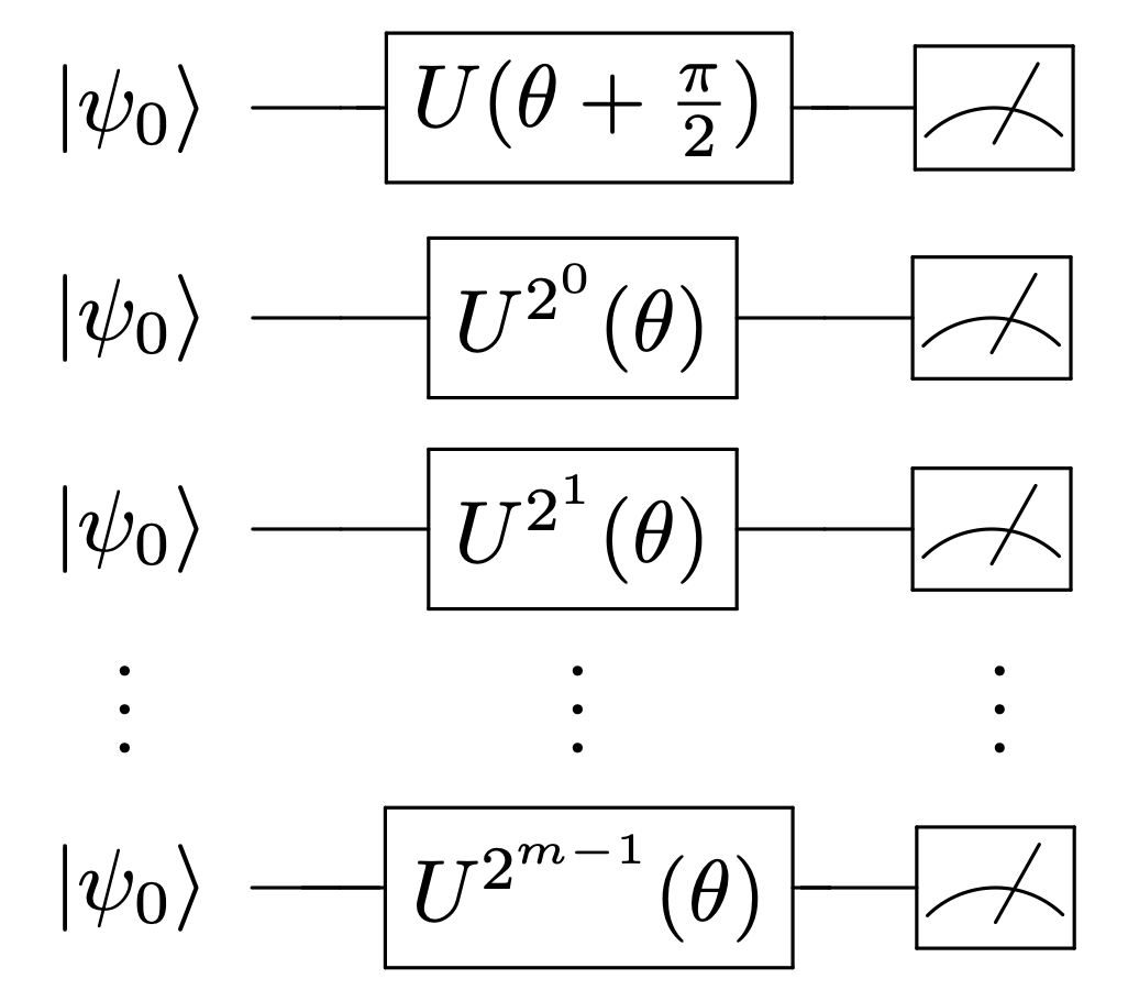
To cap the probability, $\epsilon$, that the point-identification step fails, we need to limit the probability, $\epsilon_{i}$, that the $i^{\textrm{th}}$ bit of $T$ is incorrectly assigned. Thus, the circuit with $N=2^{i}$ phase applications must be executed a minimum number of times, $\nu_{i}$. A suitable $\nu_{i}$ can be calculated using the binomial distribution’s Chernoff bound Rudolph and Grover 2003; Nielsen and Chuang 2000:

where $\delta$ is the maximum allowed absolute difference between the estimated $\widetilde{p}_{0}(N,\theta)$ and true $p_{0}(N,\theta)$. Failure occurs if $\widetilde{p}_{0}(N,\theta)>1/2$ when $p_{0}(N,\theta)<1/2$ (and vice-versa): $|\widetilde{p}_{0}(N,\theta)-p_{0}(N,\theta)|\geq|\frac{1}{2}-p_{0}(N,\theta)|$. Hence, we choose $\delta=|\frac{1}{2}-p_{0}(N,\theta)|$ when solving Eq. (7):

Problematically, one needs knowledge of $\theta$ to find $\nu_{i}$. To resolve this, we set the denominator to a constant, $\alpha\equiv 8\sec^{2}N\theta$, and accept that some values of $\theta$ lead to a failure probability larger than $\epsilon_{i}$. Increasing $\alpha$ will reduce this effect. Our protocol executes a circuit with $N=2^{i}$ in total $\nu_{i}=\alpha\ln(2/\epsilon_{i})$ times. Over the whole point-identification step, we thus apply $\hat{U}(\theta)$ a number

times in total to estimate $\theta_{\textrm{PI}}$. We now make the assertion that the whole point-identification protocol is incorrect with maximum probability $\epsilon$, such that $1-\epsilon=\prod_{i=1}^{m}(1-\epsilon_{i})$. For small $\epsilon_{i}$, $\epsilon=\sum_{i=1}^{m}\epsilon_{i}$. We use Lagrange multipliers to minimize Eq. (9) with this constraint. We find that $\epsilon_{i}=2^{i-m}\epsilon$, $\nu_{i}=\alpha\ln\left(2^{m+1-i}/\epsilon\right)$ and

To decrease $\epsilon$, each circuit is sampled a larger number of times, proportional to $\ln\left(\frac{1}{\epsilon}\right)$.

If the iteration described above is used without fine-tuning, we take $\widetilde{\theta}_{\textrm{PI}}$ as the final estimate of $\theta$. With a probability $1-\epsilon$, this estimate differs from the true $\theta$ by a truncation, with an error equal to the maximum value of the bits not estimated: $\Delta\widetilde{\theta}_{\textrm{success}}=\frac{\pi}{2^{m}}$. However, if the circuit with $N=2^{i}$ fails to identify the $(i+1)^{\textrm{th}}$ bit, this bit and the subsequent bits are incorrectly labelled. Therefore, $\widetilde{\theta}_{\textrm{PI}}$ differs from the true $\theta$ by up to twice the value of the $(i+1)^{\textrm{th}}$ bit: $\Delta\widetilde{\theta}_{\textrm{fail,i}}=\frac{\pi}{2^{i}}$. The final estimate from running the protocol once has a total mean absolute error bounded by the weighted sum of the values of $\Delta\widetilde{\theta}_{\textrm{success}}$ and $\Delta\widetilde{\theta}_{\textrm{fail,i}}$:

In the asymptotic limit, where $m$ is large, a constant $\epsilon$ leads to $\Delta\widetilde{\theta}=\mathcal{O}(m2^{-m})=\mathcal{O}\left({\log N_{\textrm{PI}}}/{N_{\textrm{PI}}}\right)$. However, choosing $\epsilon$ to be a function of $m$ allows $\Delta\widetilde{\theta}$ to decrease inversely with a larger function of $N_{\textrm{PI}}$: the choice of $\epsilon=\mathcal{O}\left(\frac{1}{m}\right)$ results in optimal scaling, with $\Delta\widetilde{\theta}=\mathcal{O}(2^{-m})$ and $N_{\textrm{PI}}=\mathcal{O}(2^{m}\log m)$. The overall mean absolute error then scales as

This scaling is a mere logarithm of a logarithm from the ideal Heisenberg Limit ²² 2 When computing the root-mean-squared error, individual errors are squared before addition. Choosing $\epsilon=\mathcal{O}(2^{-m})$ optimizes the RMS error scaling as $\log N_{\textrm{PI}}/N_{\textrm{PI}}$..

In our protocol, we combine this iterative point-identification step with the fine-tuning step, such that $N_{\textrm{max}}=2^{m}$, independent of $\epsilon$. Again, the total mean absolute error of the final estimate, $\Delta\widetilde{\theta}$, is the weighted sum of the standard deviation from success, $\sigma_{\widetilde{\theta}}$ [Eq. (6)], and the error from failure of the point-identification, $\Delta\widetilde{\theta}_{\textrm{fail,i}}$:

in the asymptotic limit. The choice of $\epsilon=\mathcal{O}\left(m^{-3/2}\right)$ results in optimal scaling, with $N_{\textrm{tot}}=\mathcal{O}(2^{m}\log m)$ and

This error scaling is a $\sqrt{\log(\log N_{\textrm{tot}})}$ improvement over our iterative point-identification alone ³³ 3 The root-mean-squared-error scaling improves similarly to $\sqrt{\log N_{\textrm{tot}}}/N_{\textrm{tot}}$.. Furthermore, in the simulations below, we see a significant reduction in the constant before the scaling.

Point identification using the QPE algorithm.—The QPE algorithm employs inverse Fourier transforms instead of MLEs to estimate $\theta$ Kitaev. To gain a $b$-bits estimate of $T=\theta/2\pi$ with an expected failure probability of $\epsilon$, $t=b+\lceil\log_{2}(2+\frac{1}{2\epsilon})\rceil$ qubits are manipulated with $N_{\textrm{tot}}=2^{t}-1$ applications of $\hat{U}(\theta)$ Nielsen and Chuang 2000. The maximum depth of the circuit is $2^{t-1}$ applications of $\hat{U}(\theta)$ plus a linear term, $\mathcal{O}(t)$, to apply the quantum Fourier transform. As such, the success probability, $1-\epsilon$, is only increased by increasing $N_{\textrm{tot}}$ and $N_{\textrm{max}}$: $N_{\textrm{tot}}\propto\frac{1}{\epsilon}$. The error scaling is the optimum Heisenberg Limit: $\Delta\widetilde{\theta}=\mathcal{O}\left(\frac{1}{N_{\textrm{tot}}}\right)$ Higgins et al. 2009. Despite the optimal scaling of the QPE algorithm, the constant factor before the scaling causes inefficiency if the failure probability is low. Furthermore, the large circuit requiring multi-qubit fully-entangled states create difficulty implementing the QPE algorithm with noisy intermediate-scale quantum hardware.

When using the QPE algorithm in the point identification step of our two-step protocol, we choose $b=m+1$. Consequently, $\hat{U}(\theta)$ is applied in total $N_{\textrm{PI}}=2^{m+1+\lceil\log_{2}(2+1/2\epsilon)\rceil}-1$ times. Equations (5) and (6) lead to

The error scaling still follows the Heisenberg Limit, but the constant before the scaling is smaller than the QPE algorithm alone. See Fig. 3(a). The largest circuit depth exceeds $N_{\textrm{max}}=2^{m+\lceil\log_{2}(2+1/2\epsilon)\rceil}=\mathcal{O}(N_{\textrm{tot}})$ in the asymptotic limit. Circuits are thus deeper than the iterative techniques described above, and use currently impractical many-probe entanglement.

Simulations.—In order to compare the performance of our two-step protocol to previous protocols, we provide numerical simulations. We choose values of $m$ and $\epsilon$ that minimize the error of an estimate, $\Delta\widetilde{\theta}$, for a given value of $N_{\textrm{tot}}$. This value of $\Delta\widetilde{\theta}$ is then plotted against $N_{\textrm{tot}}$ [Fig. 3(a)] and $N_{\textrm{max}}$ [Fig. 3(b)], for each protocol. We also set $\alpha=32$ to facilitate comparison to previous work Rudolph and Grover 2003. Figure 3(a) shows that the iterative two-step protocol diverges from the Standard Quantum Limit at $\approx 2300$ and $\approx 7$ times smaller values of $N_{\textrm{tot}}$, compared to the iterative point-identification protocol alone and the QPE algorithm alone, respectively. That is, we reach quantum advantage with fewer applications of $\hat{U}(\theta)$ than other protocols. For all simulated values of $N_{\textrm{tot}}$, our protocol produces smaller values of $\Delta\widetilde{\theta}$, compared to a protocol that conducts iterative point identification alone, as well as compared to the QPE algorithm. This happens despite our protocol having a slightly inferior asymptotic scaling compared to the QPE algorithm. Our two-step protocol with QPE-algorithm point identification achieves a lower error than the iterative two-step protocol for all simulated values of $N_{\textrm{tot}}$, but requires deeper circuits and entanglement. Figure 3(b) plots $\Delta\widetilde{\theta}$ as a function of $N_{\textrm{max}}$. The iterative two-step protocol is the most quantum-resource-efficient protocol, achieving the lowest errors with shallow circuits. To achieve an error below the Standard Quantum Limit for a given $N_{\textrm{tot}}$, the iterative method alone and the QPE algorithm alone require $N_{\textrm{max}}=2048$ and $N_{\textrm{max}}=1024$, respectively. Our two-step protocols achieve this for $N_{\textrm{max}}=2$ and $N_{\textrm{max}}=8$, when iteration and the QPE algorithm is used for point identification, respectively.

Conclusion.—We have proposed a new two-step phase-estimation protocol. In the first step, our protocol produces several contending precise estimates of an unknown phase, by sampling from a circuit with many applications of the unknown phase. Then, the protocol point identifies which estimate is in the correct parameter regime. This point identification involves independently sampling multiple circuits—each of which doubles in depth—in order to minimize the error of the final estimate of the phase with a set number of applications of the unitary operation, $N_{\textrm{tot}}$. For a given $N_{\textrm{tot}}$, our protocol achieves a lower error when compared to previous iterative protocols. Assymptotically, our protocol’s mean absolute error scales as $\mathcal{O}\left({\sqrt{\log(\log N_{\textrm{tot}})}}/{N_{\textrm{tot}}}\right)$, which is to be compared with a previously published, best, iterative scaling of $\mathcal{O}\left({\log N_{\textrm{tot}}}/{N_{\textrm{tot}}}\right)$ Rudolph and Grover 2003; de Burgh and Bartlett 2005. Furthermore, when compared to the QPE algorithm, our protocol’s circuits are shallower, independent of the failure probability, and they do not require multi-qubit entanglement. Our protocol also achieves a lower error than the QPE algorithm for currently realistic values of $N_{\textrm{tot}}$, despite having a worse asymptotic scaling. The achievement of a high precision with a shallow circuit suggests our protocol is more practical to implement in hardware-limited situations, such as noisy intermediate-scale quantum computers.

Acknowledgements.—The authors thank N. Mertig and W. Salmon for their support during this project. The authors also acknowledge support from Hitachi, Lars Hierta’s Memorial Foundation, and Girton College, Cambridge.

References

- Brassard et al. (2002) G. Brassard, P. Hoyer, M. Mosca, and A. Tapp, Contemp. Math. 305, 53 (2002).
- Shor (1994) P. Shor, in Proc. of the 35th FOCS (IEEE, New York, 1994) pp. 124–134.
- (3) S. Lloyd, S. Bosch, G. De Palma, B. Kiani, Z.-W. Liu, M. Marvian, P. Rebentrost, and D. M. Arvidsson-Shukur, quant-ph/2006.00841 .
- Harrow et al. (2009) A. W. Harrow, A. Hassidim, and S. Lloyd, Phys. Rev. Lett. 103, 150502 (2009).
- Whitfield et al. (2011) J. D. Whitfield, J. Biamonte, and A. Aspuru-Guzik, Mol. Phys. 109, 735 (2011).
- Abbott (2016) B. P. Abbott, Phys. Rev. Lett. 116, 061102 (2016).
- Rudolph and Grover (2003) T. Rudolph and L. Grover, Phys. Rev. Lett. 91, 217905 (2003).
- de Burgh and Bartlett (2005) M. de Burgh and S. D. Bartlett, Phys. Rev. A 72, 042301 (2005).
- Oblak et al. (2005) D. Oblak, P. G. Petrov, C. L. G. Alzar, W. Tittel, A. K. Vershovski, J. K. Mikkelsen, J. L. Sørensen, and E. S. Polzik, Phys. Rev. A 71, 043807 (2005).
- Giovannetti et al. (2011) V. Giovannetti, S. Lloyd, and L. Maccone, Nat. Photonics 5, 222–229 (2011).
- Lee et al. (2002) H. Lee, P. Kok, and J. P. Dowling, J. Mod. Opt. 49, 2325 (2002).
- Braunstein (1992) S. L. Braunstein, Phys. Rev. Lett. 69, 3598 (1992).
- Pezzé and Smerzi (2009) L. Pezzé and A. Smerzi, Phys. Rev. Lett. 102, 100401 (2009).
- Cleve et al. (1998) R. Cleve, A. Ekert, C. Macchiavello, and M. Mosca, Proc. R. Soc. A 454, 339 (1998).
- Nielsen and Chuang (2000) M. A. Nielsen and I. Chuang, Quantum computation and quantum information (Cambridge University Press, 2000).
- (16) E. G. Brown, O. Goktas, and W. Tham, arXiv:2006.14145 .
- Chapeau-Blondeau and Belin (2020) F. Chapeau-Blondeau and E. Belin, Ann. Telecommun. 75, 641–653 (2020).
- Giovannetti et al. (2006) V. Giovannetti, S. Lloyd, and L. Maccone, Phys. Rev. Lett. 96, 010401 (2006).
- Lewbel (2019) A. Lewbel, J. Econ. Lit. 57, 835 (2019).
- Bontemps and Magnac (2017) C. Bontemps and T. Magnac, Annu. Rev. Econom. 9, 103 (2017).
- Tamer (2010) E. Tamer, Annu. Rev. Econom. 2, 167 (2010).
- Ji et al. (2008) Z. Ji, G. Wang, R. Duan, Y. Feng, and M. Ying, IEEE Trans. Inf. Theory 54, 5172 (2008).
- Dobšíček et al. (2007) M. Dobšíček, G. Johansson, V. Shumeiko, and G. Wendin, Phys. Rev. A 76 (2007).
- Stone (1932) M. H. Stone, Ann. Math. 33, 643 (1932).
- (25) Unitaries where has explicit dependence can often be recast as such that has no dependence.
- Rice (2015) J. Rice, Mathematical statistics and data analysis (W. Ross MacDonald School Resource Services Library, 2015).
- Ly et al. (2017) A. Ly, M. Marsman, J. Verhagen, R. P. Grasman, and E.-J. Wagenmakers, J. Math. Psychol. 80, 40 (2017).
- Maccone (2013) L. Maccone, Phys. Rev. A 88, 042109 (2013).
- O’Loan (2009) C. J. O’Loan, J. Phys. A: Math. Theor. 43, 015301 (2009).
- (30) When computing the root-mean-squared error, individual errors are squared before addition. Choosing optimizes the RMS error scaling as .
- (31) The root-mean-squared-error scaling improves similarly to .
- (32) A. Y. Kitaev, arXiv:quant-ph/9511026 .
- Higgins et al. (2009) B. L. Higgins, D. W. Berry, S. D. Bartlett, M. W. Mitchell, H. M. Wiseman, and G. J. Pryde, New J. Phys. 11, 073023 (2009).