Clustering coefficients as measures of the complex interactions in a directed weighted multilayer network
Abstract
In this paper, we provide novel definitions of clustering coefficient for weighted and directed multilayer networks. We extend in the multilayer theoretical context the clustering coefficients proposed in the literature for weighted directed monoplex networks. We quantify how deeply a node is involved in a choesive structure focusing on a single node, on a single layer or on the entire system. The coefficients convey several characteristics inherent to the complex topology of the multilayer network. We test their effectiveness applying them to a particularly complex structure such as the international trade network. The trade data integrate different aspects and they can be described by a directed and weighted multilayer network, where each layer represents import and export relationships between countries for a given sector. The proposed coefficients find successful application in describing the interrelations of the trade network, allowing to disentangle the effects of countries and sectors and jointly consider the interactions between them.
Keywords:
Multilayer network , Complex systems , Clustering Coefficient , World Trade1 Introduction
The occurrence of multiple interactions within networked systems has driven the study of the multilevel nature of real-world networks. In this setting, increasing attention has been paid to heterogeneous networks in the literature. These networks have different classifications at present, including heterogeneous information networks ([21, 10]), multilayer or multiplex networks ([15, 24, 9]) and multidimensional networks ([8]). Independently of this classification, relations of a different nature are incorporated in the same complex structure. Indeed, networks usually present different characteristics in the various layers that cannot be adequately described by aggregating the layers in the overlay or the projected network (see, e.g., [7]). Furthermore, the meaning of the interconnections between nodes of different layers goes beyond a simple formal representation. These aspects prompt the study of complex structures represented by multilayer networks that preserve their original architecture as much as possible.
In this field, specific interest is posed to the triangles that a node can form across the multilayer network, . Indeed, in this case, the adjacent nodes of a node can belong to the same or to different layers (see [13]).
Since the occurrence of triangle patterns in the network is usually measured by the well-known clustering coefficient, different triangle definitions affect the expression of the clustering coefficient in multilayer systems. The clustering coefficient is in fact an important measure of network topology (see [28, 34]). In the application domain, it is meant to measure the extent to which nodes in a graph tend to cluster, representing an effective measure of “cliqueness” (see [17]).
Other definitions of the clustering coefficient in multilevel structures have been proposed (see, in particular, [15, 13, 6]) and all have revealed that an unambiguous extension is not possible in a multidimensional perspective.
These contributions focus only on undirected networks, hence neglecting directed patterns that could be relevant empirically.
Our contribution to this literature is to formulate new local clustering coefficients for weighted directed multiple networks. Since a node in a multilayer network can be clustered under different perspectives, we measure how deep a node is involved in a cohesive structure focusing on a single node, on a single layer or on the entire system. These alternative coefficients convey several characteristics inherent to the complex topology of the multilayer network.
We extend to the multilayer architecture the clustering coefficients already proposed in the literature for weighted directed monoplex networks (see [18] and [12]).
Additionally, we generalise to the directed case the coefficient provided in [15].
The proposed coefficients have been tested considering international trade data based on the World Input-Output Database ([33]). Traditionally, these data have been studied considering a monoplex structure (see, e.g., [19, 20], [25], [29, 30]) or a bipartite network (see [14], [11], [32]). However, monoplex networks, based on countries or sectors, and bipartite networks, linking countries to sectors, cannot capture the full spectrum of interactions that commonly arise between countries in the international commodity network. Relations between countries in different sectors are also neglected in multiplex trade networks without non-diagonal couplings and where nodes are countries and layers are sectors (see [26], [27], [2, 1]).
Trade data integrate different aspects, such as the occurrence of various sectors, of imports and exports. They can therefore be effectively described by a directed and weighted complex structure, where each layer represents import and export relationships between countries for a given sector. International trade data have been modelled by [5] using a weighted directed network structured on more than one layer, where each layer refers to a commodity-specific network of import/export between countries. Classical topological indicators for directed network have been studied in order to capture the statistical similarities between countries and to track how these commodity-specific networks evolve in time.
Recently, an interesting contribution ([3]) uses a suitable adaptation of eigenvector centrality in the multilayer framework to measure the economic dominance of buyers and sellers over time. The study performed by [31] on the multilayer world trade network in a given time interval reveals the particular nested structure that characterises this set of networks. This property allows to quantify the products’ complexity.
To fully take into account the architecture of trade relationships, a multilayer network is here considered in order to disentangle the effects of countries and sectors and to jointly consider the interactions between them. Indeed, modelling a complex system as a multilayer network allows to gain information that cannot be captured taking individual layers separately. Results show that the coefficients highlight the role of countries and sectors in the whole trade taking into account both inter-layer and intra-layer flows. In particular, we identify countries that are densely interconnected in all sectors and, at the same time, we bring out countries that are prominent in specific sectors. Additionally, the multilayer structure allows to unveil relevant sectors in terms of interconnection in the whole trade.
The paper is structured as follows. Section 2 reports the technical definitions related to multilayer networks. In Section 3 we formally define triangles for multilayer directed networks. Section 4 provides a new formulation of local clustering coefficients by means of supradjacency matrices. In addition, we illustrate how the new coefficients generalise the classical definitions provided in the literature for monoplex networks. Section 5 analyses the world trade network in light of the new coefficients. Conclusions follow in Section 6.
2 Preliminaries
In this section we recall some notions and definitions about directed graph [22, 4] which are essential to introduce the notation we will use in the paper.
A directed network consists of a set of vertices (or nodes) and a set of ordered pairs of elements of (arcs or directed edges). If there is an arc from node to node , then and are said to be adjacent. There is a bilateral arc between node and node if both and . A directed graph is weighted if a weight is associated with an arc in .
We represent the binary adjacency relations between couples of nodes by a square (not necessarily symmetric) matrix A of order (binary adjacency matrix), whose elements are if , otherwise.The entry represents the arc outgoing from and incoming to . Then, the ’s on the row are the arcs that leave the node . A weighted directed network is completely described by the real square matrix W of order (weighted adjacency matrix), whose elements are different from zero if , and otherwise.
In this paper we deal with node-aligned multiplex networks, with non-diagonal couplings (see [24] for the taxonomy of the multidimensional networks). The assumption that the network is non-diagonal coupled means that there may exist inter-layer arcs not only between nodes and their counterparts, but also between a node in a given layer and a node in a different layer. For short, we will adopt throughout the paper the terminology multilayer network to denote this kind of network. A multilayer network is a family of networks , where each network represents the layer and a node is adjacent to , if they are connected by an arc. Since the multilevel network is node-aligned, nodes are repeated across all levels, i.e. . Furthermore identifies all the arcs connecting nodes in the layer to nodes in the same layer (intra-layer connections) and to nodes in all the other layers (inter-layer connections). In particular, we will denote with the set of arcs from layer to , i.e. .
A weight is associated with an arc in , with . Note that when we intend that there is a weighted arc between nodes and in the layer .
A convenient way to represent the adjacency relations between pair of nodes is represented by the supradjacency matrix. It is defined as a matrix, with square blocks of order :
| (1) |
where , , are the weighted adjacency relations in the layer , whereas are the weighted adjacency relations between nodes on layers and nodes on layer . We denote the unweighted version by .
We denote the generic element of as with , where
| (2) |
Notice that the indices identify the position in the supradjacency matrix of the weight of the arc (i.e. ). Thus, from now on, we always assume this relation between and .
The in-degree of a node on layer is the number of arcs pointing towards from any layer. This degree can be expressed as follows:
| (3) |
where 1 is the -vector of ones. Definition (3) represents the -th component of the in-degree vector, with as in (2). By the definition of the matrix , is obtained as the sum of the in-degree related to arcs in the same layer and the in-degrees related to incoming arcs from other layers .
Similarly, the out-degree is:
| (4) |
The degree of a vertex in the layer is then:
| (5) |
Bilateral arcs between the node and its adjacent nodes, if any, are represented as:
| (6) |
The in-degree of a node with respect to all layers is defined as:
| (7) |
Out-degree with respect to all layers is defined similarly. The total degree on the multilayer is then .
Moving to the weighted case, the previous definitions can be replaced by the strength of a node :
| (8) |
| (9) |
The strength of a vertex in the layer is then:
| (10) |
The in-strength of a node with respect to all layers is defined as:
| (11) |
Out-strength with respect to all layers is defined similarly. The total strength of is then .
We define the strength related to bilateral arcs between the node and its adjacent nodes as:
| (12) |
Formula (12) extends formula (6) to the weighted case, multiplying each bilateral link by the arithmetic mean of its weights11 1 Other choices are possible but could be not equally effectiveness in computation.. With this choice, we are assuming that the bilateral strength sums the average weight of each bilateral arc.
3 Triangles in directed multilayer networks
To formally provide a definition of clustering coefficients in multilayer context, it is worth at first to introduce the definition of triangle.
In a multilayer, we define a triangle as a triad of nodes laying up to three different layers. Vertices in triangles can then be linked by both inter and intra-layer arcs, irrespective of their orientation. In this way, we can take into account all possible closed triads, in all inter or intra-layer directions22 2 In directed multilayer networks, triangles around a given node on layer can be classified in out, in, cycle and middleman triangles.. This definition extends to the directed case the one adopted in [6].
The number of triangles can be computed by counting the oriented -cycles around the focal node. Similarly, in a weighted directed multilayer network a weight can be given to a triangle for instance by simply multiplying the weights of its three arcs. This is not a univocal choice, and other ways to attribute weights have been proposed in the literature, giving rise to different clustering coefficients in this context.
The total number of real triangles for the node on a layer is provided by the following expression in terms of supradjacency matrix :
| (13) |
Formula (13) allows to extend the definitions on each layer and on the whole network. Indeed, the number of triangles for the node on any layer is then , and the total number of triangles in a single layer is , finally the total number of triangles in the network is .
Figure 1 illustrates what has been introduced so far on a simple example. Four nodes are connected by oriented arcs on two distinct layers. For the sake of simplicity, there are no bilateral arcs and all the weights are set equal to .

For instance we can observe that on layer node belongs to three directed triangles, whereas on layer node belongs to only two triangles. Similarly, we can calculate for each node on each level the number of actual and potential triangles.
4 Clustering coefficients in weighted directed multilayer networks
We provide here the mathematical definitions of clustering coefficients for multilayer directed networks. In this context, we can define four different types of clustering coefficients: three coefficients, depending on the node and/or layer under consideration, and a global one, relating to the entire network. Moreover, in a weighted and directed multilayer network, triangles can be weighted in more than one way, giving rise to more than one possible definition of weighted clustering coefficient.
A first possibility is to consider all actual directed triangles that a node forms with its neighbours, where the triangle’s weight is the average of the weights of the links linking a node to its adjacent nodes and . This is in line with the coefficient introduced in [12] for monoplex networks.
Hence, we define the coefficient for a node in the level as:
| (14) |
where is defined as in (1) and accordingly, are defined as in formulas (5), (10) and (12) and is the position index defined in (2).
In particular, the numerator extends to the weighted case formula (13) that counts the number of directed triangles . The denominator provides all possible (weighted) directed triangles that could form in or outside the layer .
An alternative way to weight the triangles is to use the geometric mean of the three weights of the arcs. This choice is in agreement with the coefficient proposed by [18] for monoplex networks. Hence, we define the coefficient, denoted by , as:
| (15) |
where is the matrix whose entries are , being defined as in Section 2. Elements are defined as in formulas (5) and (6) and is the position index defined as in (2).
It is noticeable that, in (14) and (15), bilateral arcs and are removed being “false” triangles, formed by and by a pair of directed arcs pointing to the same node, e.g., and . Notice that in a directed framework a node can form up to two triangles with each pair, also including two “false” potential triangles for each bilateral link.
A third possibility to assign a weight to actual and potential triangles can be found in the recent literature (see [15] and [23]). It consists in taking the product of the three weights of the symmetrised arcs, assuming that the adjacency matrix is normalised as for the coefficient in formula (15). According to this choice, the clustering coefficient can be defined as
| (16) |
where is the normalised matrix whose entries are , and are the position indices defined as in (2). The denominator in formula (16) accounts for the weights of all the connected triads centred in the node on level and it can be considered the weight of all the potential triangles. Let us notice that to the (missing or actual) arc opposite to the node of interest is assigned a weight equal to . Of course, is again the total strength of the node in level defined as in formula (10).
Formulas (14), (15) and (16) provide local coefficients, since they refer to a single node in a single layer. It turns out to be useful to define coefficients that account for an intermediate clustering structure of the network, both considering homologous nodes on different layers or all the nodes within a given layer. It is also possible to introduce an average coefficient on the whole network that traces the concept of transitivity, well-known for monolayer networks.
In order to introduce these further generalizations, we refer to formula (14) but quite naturally similar extensions of coefficients (15) and (16) can be provided.
First we can consider a single node on all the layers on which it lies. This involves calculating the total weight of triangles to which these homologous nodes belong and dividing by the potential ones:
| (17) |
where (by formula (2)) and we sum triangles over .
It is noteworthy that can be obtained as the weighted mean of the local coefficients defined in formula (14). Each local coefficient has a weight in the weighted average equal to
In other words, the more the strength (and the degree) of the node in the layer has a high incidence on the total strength (and degree) of the node in all the layers, the more affects .
Alternatively, we can focus on a single layer and define a coefficient regarding all the nodes in that layer. In particular, these nodes contribute to the coefficient on the basis of all their arcs, within the layer or outside:
| (18) |
where, again, and the sums are over .
Also in this case, the clustering coefficient for a layer can be written as the weighted mean of the local coefficients . The incidence of on depends on the relation between the strength and the degree of the node in the layer and the total strength and degree of all nodes in the layer.
Finally, we can take into account all nodes on all levels, with all their actual or potential triangles:
| (19) |
Note that formula (19) extends the definition of transitivity for the entire network to the directed multilayer case.
5 Computational experiment
5.1 Dataset, multilayer network and preliminary analyses
To test the effectiveness of the proposed coefficients, we run a computational experiment applying them to real-world data.
We refer to the international trade data collected in the World Input-Output Database (WIOD) 2016 Release ([33]). WIOD consists of a series of databases and covers 28 EU countries and 15 other major countries. Including the biggest countries
in the world, this set covers more than 85 per cent of world GDP (see, e.g., [33]). However, to complete the data and make them suitable for different modelling purposes, it is also considered a region called the Rest of the World (RoW) that collects all other countries in the world. In Table 1, we display the list of countries that are included in our analysis.
The WIOD contains annual time-series of world input–output tables covering the period from 2000 to 2014. Data consider bilateral trades of exports, expressed in millions of U.S. dollars, for each couple of origin and destination countries and distinct between 56 sectors (see Table 2 for a list of sectors). Sectors are classified according to the International Standard Industrial Classification (revision 4) (see [16]). In this analysis, we focus on the data of last available year, namely, 2014.
By these data we construct a multilayer weighted directed network, where each layer is represented by a sector. In each layer, a node corresponds to a country and a weighted arc represents the total amount of incoming or out-coming flows between a couple of countries in the same sector. In the same layer, we exclude self-loops, i.e. transaction of a country in the same sector. Inter-layer arcs are instead weighted with the amount of imports or exports between (the same or different) countries in different sectors. We obtain a multilayer network with 44 nodes and 56 sectors, represented by an asymmetric and weighted supradjacency matrix with 2464 rows and columns.
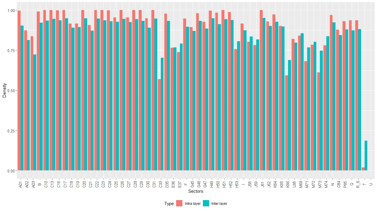
To give a first idea of the network structure, we display in Figure 2 the density of each layer and the average inter-layer density. The average inter-layer density of a sector has been computed as the average value of the densities of the graphs characterised by the connections between the sector and each other layer. It is noticeable how several sectors show a high internal density in the layer, while a lower inter-layer density is observed on average. Sector “T" (Activities of households) ) is instead very sparse and tends to be more connected with other layers. Sector “U" (Activities of extraterritorial organizations and bodies) is completely isolated having neither internal connections nor connections with other layers. Therefore, we decided to remove this layer from the network and to deal with 55 sectors.
We report in Figure 3 the total strength for each combination of sector and country. The total strength has been obtained as the sum of in and out strength of the country in the layer. It is interesting to note how manufacturing sectors (from “C10" to “C33" in the plot) are characterised by the highest volumes. In terms of country, China, USA and ROW show the highest strengths. On the one hand, China tends to be the dominant country in several sectors but shows also a strength equal to zero in specific sectors (as Repair and installation of machinery and equipment “C33", Wholesale and retail trade and repair of motor vehicles and motorcycles “G45", Publishing activities “J58", etc.). On the other hand, USA and ROW have average strength a bit lower than China but these countries show connections in all sectors.

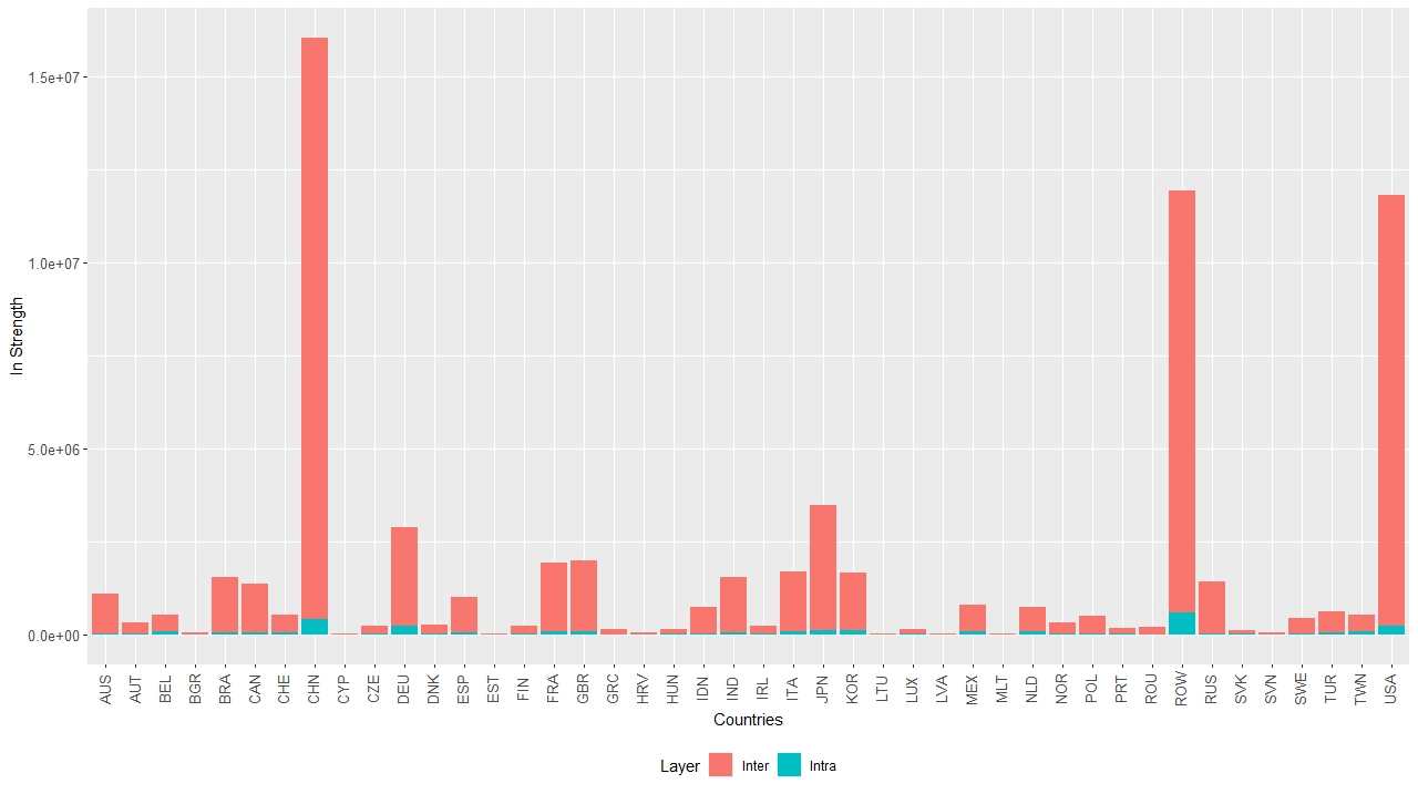
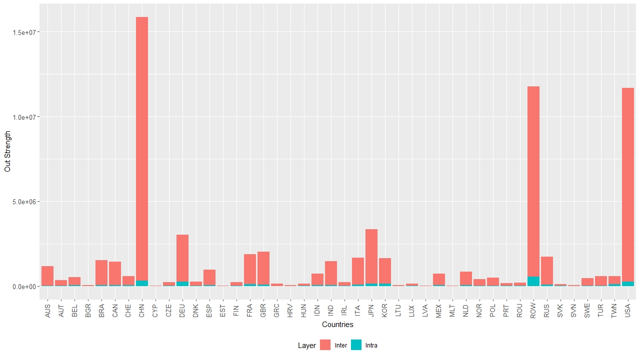
A specific focus on countries’ strength is made in Figures 4 and 5. In particular, we distinguish between in and out strength and between strength related to inter-layer and intra-layer connections. A high volume of trade due to inter-layer connections is observed. In particular, USA, AUS and CHN show the highest exposition towards inter-layer arcs. We have values lower than 3% for the ratio between the strength related to arcs in the same layer and the strength due to arcs that connect different layers. Smaller countries (as MLT, LUX, TWN, SVK, HUN) are instead more concentrated on intra-layer flows.
According to imports and exports, NOR, RUS, NLD are characterised by a positive trade balance with a ratio between in and out strength around 80%. Vice versa MLT, HUN and MEX have the opposite behaviour with the highest ratios (more than 110%).
In Figure 6 we focus on sectors’ strength. It is noticeable a very high in-strength for the sector “F" (Constructions), due in particular to directed connections with some manufacturing sectors. Important out-flows are instead observed for the sector “B" (Mining and quarrying), probably due to the use of these materials in other sectors. Finally, we observe how the sector “C26" (Manufacture of computer, electronic and optical products) is characterised by the highest intra-layer transactions, because of important trades between countries.

5.2 Main Results
We test on the multilayer network the coefficients introduced in Section 4. We compare at first the local coefficients provided by formulas (14), (15) and (16). To this end, we display in Figure 7 for each sector the ranking based on the local clustering coefficients. It allows to emphasize which countries appear prominent in terms of interconnections in each sector and, at the same time, we can appreciate different patterns between coefficients. We notice that coefficients and tend to provide similar rankings, while coefficients behave in a different way. However, it has to be stressed that values of are very close to one and hence the ranking is in this case not so interesting because very limited differences are observed between countries. Main justification is related to the fact that this coefficient is affected by the number of triangles rather than by their weights. Therefore, given the high density of the network, very few differences can be noticed between countries. Focusing on rankings given by and , it is noticeable how CHN, USA and ROW appear highly interconnected. In particular, CHN have the highest ranking in the largest number of sectors (27 and 38 sectors according to and , respectively), but USA and ROW are well connected in all sectors. We have indeed that these two countries belong to the top quartile of the clustering distribution in all sectors. We have instead that CHN shows a very low ranking in specific sectors where it is not well represented. In terms of average ranking, these countries are then followed by FRA, GBR, JAP, DEU. In particular, FRA and GBR tend to be well clustered in several sectors (especially considering the coefficient ), while JAP and DEU are instead not covered in some specific sectors. In particular, FRA has the highest ranking in sector “C33" (Air transport). France is indeed one of the largest and relevant aviation markets in Europe, because of traffic due to its size and geographic location and being home of some of the industry’s flagship names. At a lower average ranking we find ITA, RUS, KOR, NLD, ESP, countries that belong to the top quartile in specific sectors but also show a lower clustering in other sectors. It is also noteworthy how Denmark appears as a top country in sector “T", Activities of households, and Taiwan is highly interconnected in sector “C26" Manufacture of computer, electronic and optical products. Electronic component manufacturing is indeed a pillar of Taiwan’s economy, and its role is increasing over time also thanks to the development of technology.


To stress the different behaviour of the alternative clustering coefficients, we show in Figure 8 the countries’ ranking computed on the base of the three multilayer coefficients. To get these rankings, we considered the coefficients of the single node over all the layers (defined by formula (17)). We extend the comparison to the local clustering coefficients for monoplex networks. In particular, we compute on each layer a coefficient , based on the formula provided by [18] and then we average the results between the layers. Similarly, the same procedure has been applied in order to obtain the coefficient based on the formula provided in [12]. Therefore, inter-layer connections are not considered in the computation of and .
Interestingly, the inclusion of inter-layer effects produces significant disparities in the ranking. This pattern is also justified by the fact that the inter-layer connections are relevant, as shown by the behaviour of density and strength in the previous section. The coefficients referred to monoplex networks show indeed a positive rank correlation but far from one, with the results obtained from multilayer formulas. Finally, we notice a higher level of similarity between and than between and .

In Figure 9, attention has been also paid to the level of interconnection of sectors. Also in this case, the average multilayer coefficients has been compared with the monoplex versions. We notice again a positive correlation between them but with some significant differences. Focusing on specific sectors, we notice a higher level of interconnections in manufacturing sectors. In particular, sectors related to chemical, mineral, metal products and machinery and equipments (as “C20", “C23", “C25", “C28") show the highest coefficients. Other relevant sectors are wholetrade (“G46") and constructions (“F").

6 Conclusions
Clustering coefficient has gained increasing attention in network theory. In the literature several proposals have been provided for monoplex networks; however, the study of local and global clustering coefficients for multilayer networks deserves more attention.
In this paper, we focus on clustering coefficients for weighted and directed multilayer networks. The proposed coefficients generalise the alternative proposals provided in the literature for directed monoplex networks and extend existing coefficients for undirected multilayer networks.
The approach has been evaluated using the data taken from the World Input-Output DataBase. Results show the efficiency of the coefficients in capturing the degree of interconnection at different levels, emphasizing the role of countries and sectors in the whole trade taking into account both inter-layer and intra-layer flows.
References
- A. Alves et al. [2019] A. Alves, L. G., Mangioni, G., Cingolani, I., Rodrigues, F. A., Panzarasa, P., & Moreno, Y. (2019). The nested structural organization of the worldwide trade multi-layer network. Scientific Reports, 9, 2866.
- A. Alves et al. [2018] A. Alves, L. G., Mangioni, G., Rodrigues, F. A., Panzarasa, P., & Moreno, Y. (2018). Unfolding the complexity of the global value chain: Strength and entropy in the single-layer, multiplex, and multi-layer international trade networks. Entropy, 20.
- A. Alves et al. [2022] A. Alves, L. G., Mangioni, G., Rodrigues, F. A., Panzarasa, P., & Moreno, Y. (2022). The rise and fall of countries in the global value chains. Scientific Reports, 12, 9086.
- Bang-Jensen & Gutin [2008] Bang-Jensen, J., & Gutin, G. Z. (2008). Digraphs: theory, algorithms and applications. Springer Science & Business Media.
- Barigozzi et al. [2010] Barigozzi, M., Fagiolo, G., & Garlaschelli, D. (2010). Multinetwork of international trade: A commodity-specific analysis. Physical Review E, 81, 046104.
- Bartesaghi et al. [2022] Bartesaghi, P., Clemente, G. P., & Grassi, R. (2022). A tensor-based unified approach for clustering coefficients in financial multiplex networks. Information Sciences, 601, 268–286.
- Battiston et al. [2014] Battiston, F., Nicosia, V., & Latora, V. (2014). Structural measures for multiplex networks. Physical Review E, 89, 032804.
- Berlingerio et al. [2013] Berlingerio, M., Coscia, M., Giannotti, F., Monreale, A., & Pedreschi, D. (2013). Multidimensional networks: foundations of structural analysis. World Wide Web, 16, 567–593.
- Boccaletti et al. [2014] Boccaletti, S., Bianconi, G., Criado, R., Del Genio, C. I., Gómez-Gardenes, J., Romance, M., Sendina-Nadal, I., Wang, Z., & Zanin, M. (2014). The structure and dynamics of multilayer networks. Physics Reports, 544, 1–122.
- Chen et al. [2021] Chen, Z.-Y., Fan, Z.-P., & Sun, M. (2021). Tensorial graph learning for link prediction in generalized heterogeneous networks. European Journal of Operational Research, 290, 219–234.
- Cingolani et al. [2017] Cingolani, I., Panzarasa, P., & Tajoli, L. (2017). Countries’ positions in the international global value networks: Centrality and economic performance. Applied Network Science, 2.
- Clemente & Grassi [2018] Clemente, G. P., & Grassi, R. (2018). Directed clustering in weighted networks: a new perspective. Chaos, Solitons & Fractals, 107.
- Cozzo et al. [2015] Cozzo, E., Kivelä, M., De Domenico, M., Solé-Ribalta, A., Arenas, A., Gómez, S., Porter, M. A., & Moreno, Y. (2015). Structure of triadic relations in multiplex networks. New Journal of Physics, 17, 073029.
- Cristelli et al. [2013] Cristelli, M., Gabrielli, A., Tacchella, A., Caldarelli, G., & Pietronero, L. (2013). Measuring the intangibles: A metrics for the economic complexity of countries and products. PLOS ONE, 8, 1–20.
- De Domenico et al. [2013] De Domenico, M., Solé-Ribalta, A., Cozzo, E., Kivelä, M., Moreno, Y., Porter, M. A., Gómez, S., & Arenas, A. (2013). Mathematical formulation of multilayer networks. Physical Review X, 3, 041022.
- Department of Economic and Social Affairs [2008] Department of Economic and Social Affairs (2008). International Standard Industrial Classification of All Economic Activities. Technical Report United Nations.
- Ertem et al. [2016] Ertem, Z., Veremyev, A., & Butenko, S. (2016). Detecting large cohesive subgroups with high clustering coefficients in social networks. Social Networks, 46, 1–10.
- Fagiolo [2007] Fagiolo, G. (2007). Clustering in complex directed networks. Physical Review E, 76.
- Fagiolo et al. [2008] Fagiolo, G., Reyes, J., & Schiavo, S. (2008). On the topological properties of the world trade web: A weighted network analysis. Physica A: Statistical Mechanics and its Applications, 387, 3868–3873.
- Fagiolo et al. [2012] Fagiolo, G., Squartini, T., & Garlaschelli, D. (2012). Null models of economic networks: the case of the world trade web. Journal of Economic Interaction and Coordination, 8, 75–107.
- Gupta & Kumar [2020] Gupta, M., & Kumar, P. (2020). Recommendation generation using personalized weight of meta-paths in heterogeneous information networks. European Journal of Operational Research, 284, 660–674.
- Harary [1969] Harary, F. (1969). Graph theory.. Addison-Wesley, Reading, MA.
- Jia et al. [2021] Jia, M., Gabrys, B., & Musial, K. (2021). Directed closure coefficient and its patterns. PLOS ONE, 16, 1–23.
- Kivelä et al. [2014] Kivelä, M., Arenas, A., Barthelemy, M., Gleeson, J. P., Moreno, Y., & Porter, M. A. (2014). Multilayer networks. Journal of Complex Networks, 2, 203–271.
- Maluck & Donner [2015] Maluck, J., & Donner, R. V. (2015). A network of networks perspective on global trade. PLOS ONE, 10, 1–24.
- Mastrandrea et al. [2014] Mastrandrea, R., Squartini, T., Fagiolo, G., & Garlaschelli, D. (2014). Reconstructing the world trade multiplex: The role of intensive and extensive biases. Phys. Rev. E, 90, 062804.
- Menichetti et al. [2014] Menichetti, G., Remondini, D., Panzarasa, P., Mondragón, R. J., & Bianconi, G. (2014). Weighted multiplex networks. PLOS ONE, 9, 1–8.
- Newman [2003] Newman, M. E. J. (2003). The structure and function of complex networks. SIAM Review, 6, 28384. doi:10.1038/srep28384.
- Piccardi & Tajoli [2012] Piccardi, C., & Tajoli, L. (2012). Existence and significance of communities in the world trade web. Physical Review E, 85, 066119.
- Piccardi & Tajoli [2018] Piccardi, C., & Tajoli, L. (2018). Complexity, centralization, and fragility in economic networks. PLOS ONE, 13, 1–13.
- Ren et al. [2020] Ren, Z.-M., Zeng, A., & Zhang, Y.-C. (2020). Bridging nestedness and economic complexity in multilayer world trade networks. Humanities and Social Sciences Communications, 7, 1–8.
- Saracco et al. [2015] Saracco, F., Di Clemente, R., & Gabrielli, A. (2015). Randomizing bipartite networks: the case of the world trade web. Scientific Report, 5.
- Timmer et al. [2015] Timmer, M., Dietzenbacher, E., Los, B., Stehrer, R., & de Vries, G. J. (2015). An illustrated user guide to the world input–output database: the case of global automotive production. Review of International Economics, 23, 575–605.
- Watts & Strogatz [1998] Watts, D. J., & Strogatz, S. H. (1998). Collective dynamics of small-world networks. Nature, 393, 440–442.
Appendix A Lists of sectors and countries
| Number | Name | Code | Number | Name | Code |
|---|---|---|---|---|---|
| 1 | Australia | AUS | 2 | Austria | AUT |
| 3 | Belgium | BEL | 4 | Bulgaria | BGR |
| 5 | Brazil | BRA | 6 | Canada | CAN |
| 7 | Switzerland | CHE | 8 | China | CHN |
| 9 | Cyprus | CYP | 10 | Czech Republic | CZE |
| 11 | Germany | DEU | 12 | Denmark | DNK |
| 13 | Spain | ESP | 14 | Estonia | EST |
| 15 | Finland | FIN | 16 | France | FRA |
| 17 | United Kingdom | GBR | 18 | Greece | GRC |
| 19 | Croatia | HRV | 20 | Hungary | HUN |
| 21 | Indonesia | IDN | 22 | India | IND |
| 23 | Ireland | IRL | 24 | Italy | ITA |
| 25 | Japan | JPN | 26 | Korea | KOR |
| 27 | Lithuania | LTU | 28 | Luxembourg | LUX |
| 29 | Latvia | LVA | 30 | Mexico | MEX |
| 31 | Malta | MLT | 32 | Netherlands | NLD |
| 33 | Norway | NOR | 34 | Poland | POL |
| 35 | Portugal | PRT | 36 | Romania | ROU |
| 37 | Russian Federation | RUS | 38 | Slovak Republic | SVK |
| 39 | Slovenia | SVN | 40 | Sweden | SWE |
| 41 | Turkey | TUR | 42 | Taiwan | TWN |
| 43 | United States | USA | 44 | Rest of the World | ROW |
| Sector | Description | Code |
|---|---|---|
| 1 | Crop and animal production, hunting and related service activities | A01 |
| 2 | Forestry and logging | A02 |
| 3 | Fishing and aquaculture | A03 |
| 4 | Mining and quarrying | B |
| 5 | Manufacture of food products, beverages and tobacco products | C10-C12 |
| 6 | Manufacture of textiles, wearing apparel and leather products | C13-C15 |
| 7 | Manufacture of wood and of products of wood and cork, except furniture; manufacture of articles of straw and plaiting materials | C16 |
| 8 | Manufacture of paper and paper products | C17 |
| 9 | Printing and reproduction of recorded media | C18 |
| 10 | Manufacture of coke and refined petroleum products | C19 |
| 11 | Manufacture of chemicals and chemical products | C20 |
| 12 | Manufacture of basic pharmaceutical products and pharmaceutical preparations | C21 |
| 13 | Manufacture of rubber and plastic products | C22 |
| 14 | Manufacture of other non-metallic mineral products | C23 |
| 15 | Manufacture of basic metals | C24 |
| 16 | Manufacture of fabricated metal products, except machinery and equipment | C25 |
| 17 | Manufacture of computer, electronic and optical products | C26 |
| 18 | Manufacture of electrical equipment | C27 |
| 19 | Manufacture of machinery and equipment n.e.c. | C28 |
| 20 | Manufacture of motor vehicles, trailers and semi-trailers | C29 |
| 21 | Manufacture of other transport equipment | C30 |
| 22 | Manufacture of furniture; other manufacturing | C31 C32 |
| 23 | Repair and installation of machinery and equipment | C33 |
| 24 | Electricity, gas, steam and air conditioning supply | D35 |
| 25 | Water collection, treatment and supply | E36 |
| 26 | Sewerage; waste collection, treatment and disposal activities; materials recovery; remediation activities and other waste management services | E37-E39 |
| 27 | Construction | F |
| 28 | Wholesale and retail trade and repair of motor vehicles and motorcycles | G45 |
| 29 | Wholesale trade, except of motor vehicles and motorcycles | G46 |
| 30 | Retail trade, except of motor vehicles and motorcycles | G47 |
| 31 | Land transport and transport via pipelines | H49 |
| 32 | Water transport | H50 |
| 33 | Air transport | H51 |
| 34 | Warehousing and support activities for transportation | H52 |
| 35 | Postal and courier activities | H53 |
| 36 | Accommodation and food service activities | I |
| 37 | Publishing activities | J58 |
| 38 | Motion picture, video and television programme production, sound recording and music publishing activities; programming and broadcasting activities | J59 J60 |
| 39 | Telecommunications | J61 |
| 40 | Computer programming, consultancy and related activities; information service activities | J62 J63 |
| 41 | Financial service activities, except insurance and pension funding | K64 |
| 42 | Insurance, reinsurance and pension funding, except compulsory social security | K65 |
| 43 | Activities auxiliary to financial services and insurance activities | K66 |
| 44 | Real estate activities | L68 |
| 45 | Legal and accounting activities; activities of head offices; management consultancy activities | M69 M70 |
| 46 | Architectural and engineering activities; technical testing and analysis | M71 |
| 47 | Scientific research and development | M72 |
| 48 | Advertising and market research | M73 |
| 49 | Other professional, scientific and technical activities; veterinary activities | M74 M75 |
| 50 | Administrative and support service activities | N |
| 51 | Public administration and defence; compulsory social security | O84 |
| 52 | Education | P85 |
| 53 | Human health and social work activities | Q |
| 54 | Other service activities | RS |
| 55 | Activities of households as employers; undifferentiated goods- and services-producing activities of households for own use | T |
| 56 | Activities of extraterritorial organizations and bodies | U |