GradICON: Approximate Diffeomorphisms via Gradient Inverse Consistency
Abstract
We present an approach to learning regular spatial transformations between image pairs in the context of medical image registration. Contrary to optimization-based registration techniques and many modern learning-based methods, we do not directly penalize transformation irregularities but instead promote transformation regularity via an inverse consistency penalty. We use a neural network to predict a map between a source and a target image as well as the map when swapping the source and target images. Different from existing approaches, we compose these two resulting maps and regularize deviations of the Jacobian of this composition from the identity matrix. This regularizer – GradICON – results in much better convergence when training registration models compared to promoting inverse consistency of the composition of maps directly while retaining the desirable implicit regularization effects of the latter. We achieve state-of-the-art registration performance on a variety of real-world medical image datasets using a single set of hyperparameters and a single non-dataset-specific training protocol. Code is available at https://github.com/uncbiag/ICON.
1 Introduction

Image registration is a key component in medical image analysis to estimate spatial correspondences between image pairs crum2004non; sotiras2013deformable. Applications include estimating organ motion between treatment fractions in radiation therapy kessler2006image; han2021deep, capturing disease progression viergever2016survey, or allowing for localized analyses in a common coordinate system evans2012brain.
Many different registration algorithms have been proposed over the last decades in medical imaging modersitzki2003numerical; miller2006geodesic; vialard2012diffeomorphic; viergever2016survey; chen2021deep and in computer vision horn1981determining; fortun2015optical. Contributions have focused on different transformation models (i.e., what types of transformations are considered permissible), similarity measures (i.e., how “good alignment” between image pairs is quantified), and solution strategies (i.e., how transformation parameters are numerically estimated). The respective choices are generally based on application requirements as well as assumptions about image appearance and the expected transformation space. In consequence, while reliable registration algorithms have been developed for transformation models ranging from simple parametric models (e.g., rigid and affine transformations) to significantly more complex nonparametric formulations modersitzki2003numerical; miller2006geodesic; vialard2012diffeomorphic that allow highly localized control, practical applications of registration typically require many choices and rely on significant parameter tuning to achieve good performance. Recent image registration work has shifted the focus from solutions based on numerical optimization for a specific image pair to learning to predict transformations based on large populations of image pairs via neural networks yang2017quicksilver; dalca2018unsupervised; chen2021deep; ilg2017flownet; dosovitskiy2015flownet; sun2018pwc; teed2020raft; huang2022flowformer. However, while numerical optimization is now replaced by training a regression model which can be used to quickly predict transformations at test time, parameter tuning remains a key challenge as loss terms for these two types of approaches are highly related (and frequently the same). Further, one also has additional choices regarding network architectures. Impressive strides have been made in optical flow estimation as witnessed by the excellent performance of recent approaches huang2022flowformer on Sintel butler2012naturalistic. However, our focus is medical image registration, where smooth and often diffeomorphic transformations are desirable; here, a simple-to-use learning-based registration approach, which can adapt to different types of data, has remained elusive. In particular, nonparametric registration approaches require a balance between image similarity and regularization of the transformation to assure good matching at a high level of spatial regularity, as well as choosing a suitable regularizer. This difficulty is compounded in a multi-scale approach where registrations at multiple scales are used to avoid poor local solutions.
Instead of relying on a complex spatial regularizer, the recent ICON approach greer2021icon uses only inverse consistency to regularize the sought-after transformation map, thereby dramatically reducing the number of hyperparameters to tune. While inverse consistency is not a new concept in image registration and has been explored to obtain transformations that are inverses of each other when swapping the source and the target images christensen2001consistent, ICON greer2021icon has demonstrated that a sufficiently strong inverse consistency penalty, by itself, is sufficient for spatial regularity when used with a registration network. Further, as ICON does not explicitly penalize spatial gradients of the deformation field, it does not require pre-registration (e.g., rigid or affine), unlike many other related works. However, while conceptually attractive, ICON suffers from the following limitations: 1) training convergence is slow, rendering models costly to train; and 2) enforcing approximate inverse consistency strictly enough to prevent folds becomes increasingly difficult at higher spatial resolutions, necessitating a suitable schedule for the inverse consistency penalty, which is not required for GradICON.
Our approach is based on a surprisingly simple, but effective observation: penalizing the Jacobian of the inverse consistency condition instead of inverse consistency directly11 1 i.e., penalizing deviations from instead of deviations from . applies zero penalty for inverse consistent transform pairs but 1) yields significantly improved convergence, 2) no longer requires careful scheduling of the inverse consistency penalty, 3) results in spatially regular maps, and 4) improves registration accuracy. These benefits facilitate a unified training protocol with the same network structure, regularization parameter, and training strategy across registration tasks.
Our contributions are as follows:
- •
We develop GradICON (Gradient Inverse CONsistency), a versatile regularizer for learning-based image registration that relies on penalizing the Jacobian of the inverse consistency constraint and results, empirically and theoretically, in spatially well-regularized transformation maps.
- •
We demonstrate state-of-the-art (SOTA) performance of models trained with GradICON on three large medical datasets: a knee magnetic resonance image (MRI) dataset of the Osteoarthritis Initiative (OAI) nevitt2006osteoarthritis, the Human Connectome Project’s collection of Young Adult brain MRIs (HCP) van2012human, and a computed tomography (CT) inhale/exhale lung dataset from COPDGene regan2011genetic.
2 Related work
Nonparametric transformation models & regularization. There are various ways of modeling a transformation between image pairs. The most straightforward nonparametric approach is via a displacement field thirion1998image. Different regularizers for displacement fields have been proposed holden2007review, but they are typically only appropriate for small displacements modersitzki2003numerical and cannot easily guarantee diffeomorphic transformations ashburner2007fast, which is our focus here for medical image registration. Fluid models, which parameterize a transformation by velocity fields instead, can capture large deformations and, given a suitably strong regularizer, result in diffeomorphic transformations. Popular fluid models are based on viscous fluid flow christensen19943d; christensen1996deformable, the large deformation diffeomorphic metric mapping (LDDMM) model beg2005computing, or its shooting variant miller2006geodesic; vialard2012diffeomorphic. Simpler stationary fluid approaches, such as the stationary velocity field (SVF) approach arsigny2009fast; vercauteren2008symmetric, have also been developed. While diffeomorphic transformations are not always desirable, they are often preferred due to their invertibility, which allows mappings between images to preserve object topologies and prevent foldings that are physically implausible. These models have initially been developed for pair-wise image registration where solutions are determined by numerical optimization, but have since, with minimal modifications, been integrated with neural networks yang2017quicksilver; balakrishnan2019voxelmorph; shen2019networks. In a learning-based formulation, the losses are typically the same as for numerical-optimization approaches, but one no longer directly optimizes over the parameters of the chosen transformation model but instead over the parameters of a neural network which, once trained, can quickly predict the transformation model parameters.
Fluid registration models are computationally complex as they require solving a fluid equation (either greedily or via direct numerical integration miller2001group, or via scaling and squaring arsigny2009fast), but can guarantee diffeomorphic transformations. In contrast, displacement field models are computationally cheaper but make it more difficult to obtain diffeomorphic transformations. Solution regularity can be obtained for displacement field models by adding appropriate constraints on the Jacobian haber2007image. Alternatively, invertibility can be encouraged by adding inverse consistency losses, either for numerical optimization approaches christensen2001consistent or in the context of registration networks as is the case for ICON greer2021icon. Similar losses have also been used in computer vision to encourage cycle consistencies godard2017unsupervised; yin2018geonet; wang2019cycles; bian2022learning though they are, in general, not focused on spatial regularity. Most relevant to our approach, ICON greer2021icon showed that inverse consistency alone is sufficient to approximately obtain diffeomorphic transformations when the displacement field is predicted by a neural network. Our work extends this approach by generalizing the inverse consistency loss to a gradient inverse consistency loss, which results in smooth transformations, faster convergence, and more accurate registration results.
Multi-scale image registration. Finding good solutions for the optimization problems of image registration is challenging, and one might easily get trapped in an unfavorable local minimum. In particular, this might happen for self-similar images, such as lung vessels, where incorrect vessel alignment might be locally optimal. Further, if there is no overlap between vessels, a similarity measure might effectively be blind to misalignment, which is why it is important for a similarity measure to have a sufficient capture range22 2 Note that keypoint approaches hansen2021graphregnet and approaches based on optimal transport shen2021accurate can overcome some of these issues. However, in this work, we focus on the registration of images with grid-based displacement fields..
Multi-scale approaches have been proposed for optimization-based registration models studholme1995multiresolution; maes1999comparative; thevenaz2000optimization; zhao2019recursive to overcome these issues. For these approaches, the loss function is typically first optimized at a coarse resolution, and the image warped via the coarse transformation then serves as the input for the optimization at a finer resolution. This helps to avoid poor local optima, as solutions computed at coarser resolutions effectively increase capture range and focus on large-scale matching first rather than getting distracted by fine local details. Multi-scale approaches have also been used for learning-based registration eppenhof2019progressively; mok2020large; hering2019mlvirnet; jiang2020multi; de2019deep; shen2019networks and generally achieve better results than methods that only consider one scale balakrishnan2019voxelmorph. These methods all use sub-networks operating at different scales but differ in how the multi-scale strategy is incorporated into the network structure and the training process. A key distinction is if source images are warped as they pass through the different sub-networks hering2019mlvirnet; mok2020large; de2019deep; greer2021icon or if sub-networks always start from the unwarped, albeit downsampled, source image eppenhof2019progressively. The former approach simplifies capturing large deformations as sub-networks only need to refine a transformation rather than capturing it in its entirety. However, these methods compute the similarity measure and the regularizer losses at all scales, which requires balancing the weights of the losses across all scales and for each scale between the similarity measure and the regularizer. Hence, there are many parameters that are difficult to tune. To side-step the tuning issue, it is common to rely on a progressive training protocol to avoid tuning the weights between losses at all scales. We find that our multi-resolution approach trains well when the loss and regularizer are applied only at the highest scale: the coarser components are effectively trained by gradients propagating back through the multi-scale steps.
3 Gradient Inverse Consistency (GradICON)
3.1 Preliminaries
We denote by and the source and the target images in our registration problem. By we denote a transformation map with the intention that . The map is a diffeomorphism if it is differentiable, bijective and its inverse is differentiable as well33 3 Basically, we are interested in properties of , as this is the region that can affect the image similarity, but since many maps (e.g., translations) carry points outside of , must be defined at those points for to be defined on all of . In practice, this is achieved for a displacement field by . . Optimization-based image registration approaches typically solve the optimization problem
| (1) |
where is the similarity measure, is a regularizer, are the transformation parameters, and . In learning-based registration, one does not directly optimize over the transformation parameters of , but instead over the parameters of a neural network that predicts given the source and target images. Such a network is trained over a set of image pairs by solving
|
|
(2) |
with as shorthand for denoting the output of the network given the -th input image pair. By training with and the loss is symmetric in expectation. For ease of notation, we omit the subscripts or in cases where the dependency is clear from the context.
3.2 Regularization
Picking a good regularizer is essential as it implicitly expresses the class of transformations one considers plausible for a registration. Ideally, the space of plausible transformations should be known (e.g., based on physical principles) or learned from the data. As nonparametric image registration (at least for image pairs) is an ill-posed problem fischer2008ill, regularization is required to obtain reasonable solutions.
Regularizers frequently involve spatial derivatives of various orders to discourage spatial non-smoothness holden2007review. This typically requires picking a type of differential operator (or, conversely, a smoothing operator) as well as all its associated parameters. Most often, this regularizer is chosen for convenience and not learned from data. Instead of explicitly penalizing spatial non-smoothness, ICON greer2021icon advocates using inverse consistency as a regularizer, which amounts to learning a transformation space from data in the class of (approximately) invertible transforms. When implementing inverse consistency, there is a choice of loss. The ICON approach penalizes the sum-of-squares difference between the identity and the composition of the maps between images and , i.e., the regularizer has the form where denotes the identity transform. In greer2021icon, it is shown that this loss has an implicit regularization effect, similar to a sum-of-squares on the gradient of the transformation, i.e., an type of norm. In fact, it turns out that regular invertible maps can be learned without explicitly penalizing spatial gradients. Inspired by this observation, we propose to use the Jacobian () of the composition of the maps instead, i.e.,
| (3) |
where the identity matrix, and is the squared Frobenius norm integrated over . As we will see in Section 5, this loss equally leads to regular maps by exerting another form of implicit regularization, which we analyze in Section 3.3. To understand the implicit regularization of the ICON loss, one makes the modeling choice such that , i.e., the output of the network is inverse consistent up to a white noise term with parameter (artificially introduced to make the discussion clear). This white noise can be used to prove that the resulting maps are regularized via the square of a first-order Sobolev (semi-) norm. Further, greer2021icon empirically showed that an approximate diffeomorphism can be obtained without the white noise when used in the context of learning a neural registration model: if inverse consistency is not exactly enforced, as suggested above, the inconsistency can be modeled by noise, and the observed smoothness is explained by the theoretical result. In our analysis, we follow a conceptually similar idea.
3.3 Analysis
Implicit type regularization. Since the GradICON loss of Eq. 3 is formulated in terms of the gradient, it is a natural assumption to put the white noise on the Jacobians themselves rather than on the maps, i.e., where is a white noise. This model of randomness is motivated by the stochastic gradient scheme on the global population that drives the parameters of the networks. At the level of maps, we write where . Since integration is a low-pass filter, the noise applies to the low frequencies of . In addition, we expect the low frequencies of the noise to be dampened by the similarity measure between and . Hence, we hypothesize that , which will be used only once in our analysis. This comparison means that our estimates of the gradient and on our grid satisfy this inequality. We assess this hypothesis Section A.1. We start by rewriting the GradICON regularizer , by applying the chain rule, as
| (4) |
using and still omitting the integral sign. We now Taylor expand the loss w.r.t. and in particular expand the term from Eq. 4 as
| (5) |
where implies that the approximation
| (6) |
holds as it is only compared with in the expansion. Using the first-order approximation , see Appendix A.1, and simplifying Eq. (4), we obtain
|
|
(7) |
as (and selecting the first-order coefficients in ). Expanding the square then yields
|
|
(8) |
Under the assumption of independence of the white noises and , the contribution of the last term in Eq. 8 vanishes in expectation. We are left with the following loss, at order , now taking expectation,
|
|
(9) |
Note that the expectation is explicit due to the white noise assumption; thus, Eq. 9 can be further simplified to
|
|
(10) |
Eq. 10 amounts to an regularization of the inverse of the Jacobian maps on and which explains why we call it type of regularization, see Appendix A.1; yet, strictly speaking, it is not the standard norm mang2016H1.
Comparison with ICON greer2021icon. Interestingly, our analysis shows that GradICON is an type of regularization as for ICON, although we could have expected a second-order regularization from the model. Such higher-order terms appear when taking into account the magnitude of the noise in the expansion. While there are several assumptions that can be formulated differently, such as the form of the noise and the fact that it is white noise for given pairs of images , we believe that Eq. 10 is a plausible explanation of the observed regularity of the maps in practice. Importantly, since this regularization is implicit, GradICON, as well as ICON can learn based on a slightly more informative prior than this regularization which relies on simplifying assumptions.
Why GradICON performs better than ICON. In practice, we observe that learning a registration model via the GradICON regularizer of Eq. 3 shows a faster convergence than using the ICON regularizer, not only in the toy experiment of Sec. 5.4 but also on real data. While we do not yet have a clear explanation for this behavior, we provide insight based on the following key differences between the two variants.
First, a difference by a translation is not penalized in the GradICON formulation, but implicitly penalized in the similarity measure, assuming images are not periodic. Second, using the Jacobian in Eq. 3 correlates the composition of the map between neighboring voxels. In a discrete (periodic) setting, this can be seen by expanding the squared norm. To shorten notations, define considered as a discrete vector. Then, Eq. 3 is the sum over voxels , which can be rewritten as
| (11) |
where is the (hyper-)parameter for the finite difference estimation of the gradient. This shows that the GradICON regularizer includes more correlation than the ICON regularizer, which would only contain the first factor in Eq. 11. Lastly, it is known Charpiat2007 that gradient descent on an energy rather than energy is a preconditioning of the gradient flow, emphasizing high-frequencies over low-frequencies. In our case, however, high-frequencies are the dominant cause of folds. Consequently, as GradICON penalizes high frequencies but allows low frequencies of the composition of the maps to deviate from identity, this is beneficial to avoid folds44 4 Indeed, the neighborhood of identity of invertible maps is much larger for small-frequency perturbations than for high-frequency perturbations; what matters for invertibility is the norm of the gradient.. Overall, GradICON is more flexible than ICON while retaining the non-folding behavior of the resulting maps.
4 Implementation
To learn a registration model under Eq. 3, we use a neural network that predicts the transformation maps. In particular, we implement a multi-step (i.e., multiple steps within a forward pass), multi-resolution approach trained with a two-stage process, followed by optional instance optimization at test time. We will discuss these parts next.
4.1 Network structure
To succinctly describe our network structure, we henceforth omit and represent a registration neural network as (or e.g. ). The notation (shorthand for ) represents the output of this network (a transform from ) for input images and . To combine such registration networks into a multistep, multiscale approach, we rely on the following combination operators from greer2021icon:
|
|
The downsample operator (Down) is for predicting the warp between two high-resolution images using a network that operates on low-resolution images, and the two-step operator (TS) is for predicting the warp between two images in two steps, first capturing the coarse transform via and then the residual transform via . We use these operators to realize a multi-resolution, multi-step network, see Fig. 2, via
| (12) | ||||
Our atomic (i.e., not composite) registration networks are each represented by a UNet instance55 5 For reference, networks.tallUnet2 in the ICON source code. from greer2021icon taking as input two images and returning a displacement field . These displacement fields are converted to functions since the above operators are defined on networks that return functions from to .
4.2 Training
We define a single training protocol that is applied to train a network on all the registration tasks of Sec. 5. For preprocessing, each image has its intensity clipped and rescaled to , with clipping intensities appropriate for the modality and anatomy being registered. For modalities with region of interest (ROI) annotations (brain and lung), all values outside the region of interest are set to zero. For intra-subject registration, we have many fewer pairs to train on66 6 For intra-subject reg., dataset size instead of )., so we perform augmentation via random flips along axes and small affine warps (see Section A.2). In all experiments, the image similarity measure is combined with the GradICON regularizer to yield the overall loss
| (13) |
In our implementation, is computed using one-sided finite differences with 1e-3, is computed by (uniform) random sampling over with number of samples equal to the number of voxels in the image , and we use coordinates where .
Multi-stage training. We train in two stages. Stage1: we train the multi-resolution network defined in Eq. 12 with the loss from Eq. 13. Stage2: we train with the same loss, jointly optimizing the parameters of Stage1 and .
Instance optimization. We optionally optimize the loss of Eq. 13 for 50 iterations at test time wang2022PLOSL. This typically improves performance but also increases runtime.
Unless noted otherwise, we use LNCC (local normalized cross-correlation) with a Gaussian kernel (std. of 5 voxels), computed as in vishnevskiy2017isotropic, and GradICON with balancing parameter . Stage1 and Stage2 are trained using ADAM at a learning rate of 5e-5 for 50,000 iterations each. This protocol remains fixed across all datasets, and any result obtained by exactly this protocol is marked by ; if instance optimization is included, results are marked by .
5 Experiments
Ethics. We use one 2D synthetic (Triangles and Circles), one real 2D (DRIVE), and four real 3D datasets (OAI, HCP, COPDGene, DirLab). Acquisitions for all real datasets were approved by the respective Institutional Review Boards.
5.1 Datasets
Triangles and Circles. A synthetic 2D dataset introduced in greer2021icon where images are either triangles or circles. We generate 2000 hollow images with size which consist of the shape edges and use them as the training set.
DRIVE staal2004ridge. This 2D dataset contains 20 retina images and the corresponding vessel segmentation masks. We use the segmentation masks to define a synthetic registration problem. In particular, we take downsampled segmentations as the source (/target) image and warp them with random deformations generated by ElasticDeform77 7 https://zenodo.org/badge/latestdoi/145003699 to obtain the corresponding target (/source) image. We generate 20 pairs per image, leading to 400 pairs at size in total.
OAI nevitt2006osteoarthritis. We use a subset of 2532 images from the full corpus of MR images of the Osteoarthritis Initiative (OAI88 8 https://nda.nih.gov/oai) for training and 301 pairs of images for testing. The images are normalized so that the th percentile and the th percentile of the intensity are mapped to 0 and 1, respectively. Then we clamp the normalized intensity to be in . We follow the train-test split99 9 Available at https://github.com/uncbiag/ICON used in greer2021icon; shen2019networks. We downsample images from to
HCP van2012human. We use a subset of T1-weighted and brain-extracted images of size from the Human Connectome Project’s (HCP) young adult dataset to assess inter-patient brain registration performance. We downsample images to for training but evaluate the average Dice score for 28 manually segmented subcortical brain regions rushmore2022anatomically; rushmore_r_jarrett_2022_dataset1010 10 https://doi.org/10.5281/zenodo.6967315 at the original resolution. We train on 1076 images, excluding the 44 images we use for testing.
COPDGene regan2011genetic. We use a subset of 1111 11 The dataset contains 1000 pairs, but 1 pair is also in the DirLab challenge set, and so was excluded from training. 999 inspiratory-expiratory lung CT pairs from the COPDGene study1212 12 https://www.ncbi.nlm.nih.gov/gap regan2011genetic with provided lung segmentation masks for training. The segmentation masks are computed automatically1313 13 shorturl.at/ciEW6. CT images are first resampled to isotropic spacing (2mm) and cropped/padded evenly along each dimension to obtain a volume. Hounsfield units are clamped within and scaled linearly to . Then, the lung segmentations are applied to the images to extract the lung region of interest (ROI). Among the processed data, we use 899 pairs for training and 100 pairs for validation.
DirLabcastillo2013reference. This dataset is only used to evaluate a trained network. It contains 10 pairs of inspiration-expiration lung CTs with 300 anatomical landmarks per pair, manually identified by an expert in thoracic imaging. We applied the same preprocessing and lung segmentation as for COPDGene.
5.2 Ablation study
In Table 1, we investigate 1) which UNet structure should be used and 2) how multi-resolution, multi-stage training, instance optimization, and data augmentation affect the registration results. To this end, we train on COPDGene and evaluate on DirLab using the same similarity measure, regularizer weight , and number of iterations. We report the mean target registration error (mTRE) on landmarks (in mm) and the percentage of voxels with negative Jacobian ().
| Backbone | Res. | 2nd | Opt. | Aug. | mTRE | |
|---|---|---|---|---|---|---|
| (in mm) | ||||||
| UNet from balakrishnan2019voxelmorph | 1 | 17.582 | 0.01440 | |||
| UNet from greer2021icon | 1 | 5.412 | 0.00014 | |||
| 3 | 3.259 | 0.00109 | ||||
| 3 | ✓ | 2.587 | 0.00032 | |||
| 3 | ✓ | 3.182 | 0.00042 | |||
| 3 | ✓ | ✓ | 1.378 | 0.00021 | ||
| 3 | ✓ | ✓ | 1.932 | 0.00026 | ||
| 3 | ✓ | ✓ | ✓ | 1.314 | 0.00023 |
First, we observe that the UNet from greer2021icon performs better than the UNet from balakrishnan2019voxelmorph. Hence, in all experiments, we adopt the former as our backbone. Notably, this model has considerably more parameters than the variant from balakrishnan2019voxelmorph ( 17M vs. 300k, see Section A.6), but uses less V-RAM as it concentrates parameters in the heavily downsampled layers of the architecture. Second, we find that the multi-resolution approach, including Stage2 training, clearly improves performance, reducing the mTRE from 5.412mm to 3.259mm (1 vs. 3 res.) and further down to 3.182mm (with Stage2). In this setting, there is also a noticeable benefit of (affine) data augmentation, with the mTRE dropping to 1.932mm. This is not unexpected, though, as we only have 899 pairs of training images for this (inter-patient) registration task. While this is considered a large corpus for medical imaging standards, it is small from the perspective of training a large neural network. Finally, we highlight that adding instance optimization yields the overall best results, but the benefits are less noticeable in combination with augmentation.
5.3 Comparison to other regularizers
We study different regularizers in terms of the trade-off between transform regularity and image similarity on the training set when varying . We use Stage1 from Eq. 12 for all experiments, setting the regularizer to either Bending Energy (), Diffusion (), ICON, or GradICON.
Specifically, we pick for each regularizer such that is kept at roughly the same level and train multiple networks with for the same number of iterations. Fig. 3 shows results on Triangles and Circles and DRIVE. We observe that all the regularizers lose a certain level of accuracy when increasing and GradICON in general has the least sacrifice in similarity. This is presumably because of the possible magnitude of deformation each regularizer allows. More results can be found in Section A.3.
5.4 Empirical convergence analysis
To demonstrate improved convergence when training models with our GradICON regularizer vs. models trained with the ICON regularizer of greer2021icon, we assess the corresponding loss curves under the same network architecture, in particular, the network described in Sec. 4. We are specifically interested in (training) convergence behavior when both models produce a similar level of map regularity. To this end, we choose to approximately achieve the same similarity loss under both regularizers and plot the corresponding curves for , see Fig. 4, for Triangles and Circles and DRIVE.
Overall, we see that GradICON converges significantly faster than ICON. We hypothesize that this is due to the fact that maps produced by GradICON contain larger motions than maps produced by ICON. I.e., for the same level of regularity, ICON more strongly limits deformations, effectively slowing down and resulting in less accurate image alignments.
5.5 Inter-patient registration
We evaluate inter-patient registration performance of our model with GradICON regularization on OAI and HCP. We report (as in Section 5.2) and the mean DICE score between warped and target image for the segmentations of the femoral and tibial cartilage (OAI), and of a set of 28 subcortical brain regions (HCP). Both measures, averaged over the evaluation data, are listed in Table 2. In particular, we compare GradICON to the methods reported in shen2019networks and greer2021icon on OAI, and compare to ANTs SyN avants2008symmetric and SynthMorph hoffmann2022synthmorph1414 14 Using SynthMorph networks trained on HCP aging data, which differs slightly from the HCP Young Adults data we use; see harms2018972 for a comparison. (sm-shapes/brains) on HCP. Segmentations are not used during training and allow quantifying if the network yields semantically meaningful registrations. Table 2 shows that on the OAI dataset GradICON can significantly outperform the state-of-the-art with minimal parameter tuning and, just as ICON, without the need for affine pre-alignment (i.e., a step needed by many registration methods on OAI). On HCP, GradICON performs better than the standard non-learning approach (SyN) and matches SynthMorph while not requiring affine pre-alignment and producing much less folds.
| Method | Trans. | DICE | |||
|---|---|---|---|---|---|
| OAI | |||||
| Initial | 7.6 | ||||
| Demons vercauteren2009diffeomorphic | A,DVF | Gaussian | MSE | 63.5 | 0.0006 |
| SyN avants2008symmetric | A,VF | Gaussian | LNCC | 65.7 | 0.0000 |
| NiftyReg modat2010fast | A,B-Spline | BE | NMI | 59.7 | 0.0000 |
| NiftyReg modat2010fast | A,B-Spline | BE | LNCC | 67.9 | 0.0068 |
| vSVF-opt shen2019networks | A,vSVF | m-Gauss | LNCC | 67.4 | 0.0000 |
| VM balakrishnan2019voxelmorph | SVF | Diff. | MSE | 46.1 | 0.0028 |
| VM balakrishnan2019voxelmorph | A,SVF | Diff. | MSE | 66.1 | 0.0013 |
| AVSM shen2019networks | A,vSVF | m-Gauss | LNCC | 68.4 | 0.0005 |
| ICON* greer2021icon | DVF | ICON | MSE | 65.1 | 0.0040 |
| Ours (MSE, ) | DVF | GradICON | MSE | 69.5 | 0.0000 |
| Ours (MSE, , Opt.) | DVF | GradICON | MSE | 70.5 | 0.0001 |
| Ours (std. protocol) | DVF | GradICON | LNCC | 70.1 | 0.0261 |
| DVF | GradICON | LNCC | 71.2 | 0.0042 | |
| HCP | |||||
| Initial | 53.4 | ||||
| FreeSurfer-Affine∗ reuter2010highly | A | — | TB | 62.1 | 0.0000 |
| SyN∗ avants2008symmetric | A,VF | Gaussian | MI | 75.8 | 0.0000 |
| sm-shapes∗ hoffmann2022synthmorph | A,SVF | Diff. | DICE | 79.8 | 0.2981 |
| sm-brains∗ hoffmann2022synthmorph | A,SVF | Diff. | DICE | 78.4 | 0.0364 |
| Ours (std. protocol) | DVF | GradICON | LNCC | 78.7 | 0.0012 |
| DVF | GradICON | LNCC | 80.5 | 0.0004 | |
| DirLab | |||||
| Method | Trans. | mTRE | |||
| (in mm) | |||||
| Initial | 23.36 | ||||
| SyN avants2008symmetric | A,VF | Gaussian | LNCC | 1.79 | — |
| Elastix klein2009elastix | A,B-Spline | BE | MSE | 1.32 | — |
| NiftyReg modat2010fast | A,B-Spline | BE | MI | 2.19 | — |
| PTVReg vishnevskiy2017isotropic | DVF | TV | LNCC | 0.96 | — |
| RRN he2021recursive | DVF | TV | LNCC | 0.83 | — |
| VM∗ balakrishnan2019voxelmorph | A,SVF | Diff. | NCC | 9.88 | 0.0000 |
| LapIRN∗ mok2020large | SVF | Diff. | NCC | 2.92 | 0.0000 |
| LapIRN∗ mok2020large | DVF | Diff. | NCC | 4.24 | 0.0105 |
| Hering et al. hering2021cnn | DVF | Curv+VCC | DICE | 2.00 | 0.0600 |
| +KP | |||||
| +NGF | |||||
| GraphRegNet hansen2021graphregnet | DV | — | MSE | 1.34 | — |
| PLOSL wang2022PLOSL | DVF | Diff. | TVD | 3.84 | 0.0000 |
| +VMD | |||||
| wang2022PLOSL | DVF | Diff. | TVD | 1.53 | 0.0000 |
| +VMD | |||||
| ICON∗ greer2021icon | DVF | ICON | LNCC | 7.04 | 0.3792 |
| Ours (std. protocol) | DVF | GradICON | LNCC | 1.93 | 0.0003 |
| DVF | GradICON | LNCC | 1.31 | 0.0002 | |
5.6 Intra-patient registration
We demonstrate the ability of our model with GradICON regularization to predict large deformations between lung exhale (source)/inhale (target) pairs (within patient) from COPDGene. This dataset is challenging as deformations are complex and large. Motion is primarily visually represented by the deformation of lung vessels, which form a complex tree-like structure that creates capture-range and local minima challenges for registration. As in our ablation study (Section 5.2), we report and the mTRE (in mm) for manually annotated lung vessel landmarks castillo2013reference averaged over all 10 DirLab image pairs. We assess GradICON against traditional optimization-based methods and state-of-the-art (SOTA) learning-based methods. Among the learning-based methods, VM balakrishnan2019voxelmorph, LapIRN mok2020large, Hering el al. hering2021cnn and PLOSL wang2022PLOSL are trained on a large dataset and evaluated on the unseen test dataset. GraphRegNet hansen2021graphregnet has been evaluated on a small dataset with 5-fold cross validation. wang2022PLOSL is PLOSL with instance optimization, which is comparable to GradICON. Table 2 shows that our performance (1.93mm) in a single forward pass is the best of any one-forward-pass neural method that has been trained on a large dataset and is evaluated on an unseen test set. our approach with instance optimization (1.31mm) exceeds the SOTA for learning-based approaches of any sort and performs slightly worse than the best optimization-based methods.
6 Conclusion
We introduced and theoretically analyzed GradICON, a new regularizer to train deep image registration networks. In contrast to ICON greer2021icon, GradICON penalizes the Jacobian of the inverse consistency constraint. This has profound effects: we obtain dramatically faster training convergence, higher registration accuracy, do not require scale-dependent regularizer tuning, and retain desirable implicit regularization effects resulting in approximately diffeomorphic transformations. Remarkably, this allows us to train registration networks using GradICON regularization with one standard training protocol for a range of different registration tasks. In fact, using this standard training protocol, we match or outperform state-of-the-art registration methods on three challenging and diverse 3D datasets. This uniformly good performance without the need for dataset-specific tuning takes the pain out of training deep 3D registration networks and makes our approach highly practical.
Limitations and future work. We only explored first-order derivatives of the inverse-consistency constraint and intensity-based registration. This might have limited registration performance. Studying higher-order derivatives, more powerful image similarity measures (e.g., based on deep features), as well as extensions to piecewise diffeomorphic transformations would be interesting future work.
7 Acknowledgements
This work was supported by NIH grants 1R01AR072013, 1R01HL149877, 1R01EB028283, RF1MH126732, R41MH118845, R01MH112748, R01NS125307, and 5R21LM013670. The work expresses the views of the authors, not of NIH. Roland Kwitt was supported in part by the Austrian Science Fund (FWF): project FWF P31799-N38 and the Land Salzburg (WISS 2025) under project numbers 20102- F1901166-KZP and 20204-WISS/225/197-2019. The knee imaging data were obtained from the controlled access datasets distributed from the Osteoarthritis Initiative (OAI), a data repository housed within the NIMH Data Archive. OAI is a collaborative informatics system created by NIMH and NIAMS to provide a worldwide resource for biomarker identification, scientific investigation and OA drug development. Dataset identifier: NIMH Data Archive Collection ID: 2343. The brain imaging data were provided by the Human Connectome Project, WU-Minn Consortium (Principal Investigators: David Van Essen and Kamil Ugurbil; 1U54MH091657) funded by the 16 NIH Institutes and Centers that support the NIH Blueprint for Neuroscience Research; and by the McDonnell Center for Systems Neuroscience at Washington University. The lung imaging data was provided by the COPDGene study.
References
- (1) Vincent Arsigny, Olivier Commowick, Nicholas Ayache, and Xavier Pennec. A fast and log-Euclidean polyaffine framework for locally linear registration. J. Math. Imaging Vis., 33(2):222–238, 2009.
- (2) John Ashburner. A fast diffeomorphic image registration algorithm. Neuroimage, 38(1):95–113, 2007.
- (3) Brian B Avants, Charles L Epstein, Murray Grossman, and James C Gee. Symmetric diffeomorphic image registration with cross-correlation: evaluating automated labeling of elderly and neurodegenerative brain. MedIA, 12(1):26–41, 2008.
- (4) Guha Balakrishnan, Amy Zhao, Mert R Sabuncu, John Guttag, and Adrian V Dalca. VoxelMorph: a learning framework for deformable medical image registration. TMI, 38(8):1788–1800, 2019.
- (5) M Faisal Beg, Michael I Miller, Alain Trouvé, and Laurent Younes. Computing large deformation metric mappings via geodesic flows of diffeomorphisms. IJCV, 61(2):139–157, 2005.
- (6) Zhangxing Bian, Allan Jabri, Alexei A Efros, and Andrew Owens. Learning pixel trajectories with multiscale contrastive random walks. In CVPR, 2022.
- (7) Daniel J Butler, Jonas Wulff, Garrett B Stanley, and Michael J Black. A naturalistic open source movie for optical flow evaluation. In ECCV, 2012.
- (8) Richard Castillo, Edward Castillo, David Fuentes, Moiz Ahmad, Abbie M Wood, Michelle S Ludwig, and Thomas Guerrero. A reference dataset for deformable image registration spatial accuracy evaluation using the COPDgene study archive. Phys. Med. Biol., 58(9):2861, 2013.
- (9) Guillaume Charpiat, Pierre Maurel, Jean-Philippe Pons, Renaud Keriven, and Olivier Faugeras. Generalized gradients: Priors on minimization flows. IJCV, 73:325–344, 07 2007.
- (10) Xiang Chen, Andres Diaz-Pinto, Nishant Ravikumar, and Alejandro F Frangi. Deep learning in medical image registration. Prog. biomed. eng., 3(1):012003, 2021.
- (11) Gary E Christensen and Hans J Johnson. Consistent image registration. TMI, 20(7):568–582, 2001.
- (12) Gary E Christensen, Richard D Rabbitt, and Michael I Miller. 3D brain mapping using a deformable neuroanatomy. Phys. Med. Biol., 39(3):609, 1994.
- (13) Gary E Christensen, Richard D Rabbitt, and Michael I Miller. Deformable templates using large deformation kinematics. TMI, 5(10):1435–1447, 1996.
- (14) William R Crum, Thomas Hartkens, and DLG Hill. Non-rigid image registration: theory and practice. Brit. J. Radiol., 77(suppl_2):S140–S153, 2004.
- (15) Adrian V Dalca, Guha Balakrishnan, John Guttag, and Mert R Sabuncu. Unsupervised learning for fast probabilistic diffeomorphic registration. In MICCAI, 2018.
- (16) Bob D De Vos, Floris F Berendsen, Max A Viergever, Hessam Sokooti, Marius Staring, and Ivana Išgum. A deep learning framework for unsupervised affine and deformable image registration. MedIA, 52:128–143, 2019.
- (17) Alexey Dosovitskiy, Philipp Fischer, Eddy Ilg, Philip Hausser, Caner Hazirbas, Vladimir Golkov, Patrick Van Der Smagt, Daniel Cremers, and Thomas Brox. Flownet: Learning optical flow with convolutional networks. In CVPR, 2015.
- (18) Koen AJ Eppenhof, Maxime W Lafarge, Mitko Veta, and Josien PW Pluim. Progressively trained convolutional neural networks for deformable image registration. TMI, 39(5):1594–1604, 2019.
- (19) Alan C Evans, Andrew L Janke, D Louis Collins, and Sylvain Baillet. Brain templates and atlases. Neuroimage, 62(2):911–922, 2012.
- (20) Bernd Fischer and Jan Modersitzki. Ill-posed medicine—an introduction to image registration. Inverse problems, 24(3):034008, 2008.
- (21) Denis Fortun, Patrick Bouthemy, and Charles Kervrann. Optical flow modeling and computation: A survey. Comput. Vis. Image Underst., 134:1–21, 2015.
- (22) Clément Godard, Oisin Mac Aodha, and Gabriel J Brostow. Unsupervised monocular depth estimation with left-right consistency. In CVPR, 2017.
- (23) Hastings Greer, Roland Kwitt, François-Xavier Vialard, and Marc Niethammer. ICON: Learning regular maps through inverse consistency. In ICCV, 2021.
- (24) Eldad Haber and Jan Modersitzki. Image registration with guaranteed displacement regularity. IJCV, 71(3):361–372, 2007.
- (25) Xu Han, Jun Hong, Marsha Reyngold, Christopher Crane, John Cuaron, Carla Hajj, Justin Mann, Melissa Zinovoy, Hastings Greer, Ellen Yorke, Gig Mageras, and Marc Niethammer. Deep-learning-based image registration and automatic segmentation of organs-at-risk in cone-beam CT scans from high-dose radiation treatment of pancreatic cancer. J. Med. Phys., 48(6):3084–3095, 2021.
- (26) Lasse Hansen and Mattias P Heinrich. GraphRegNet: Deep graph regularisation networks on sparse keypoints for dense registration of 3D lung CTs. TMI, 40(9):2246–2257, 2021.
- (27) Michael P Harms, Leah H Somerville, Beau M Ances, Jesper Andersson, Deanna M Barch, Matteo Bastiani, Susan Y Bookheimer, Timothy B Brown, Randy L Buckner, Gregory C Burgess, Timothy S Coalson, Michael A Chappell, Mirella Dapretto, Gwenaëlle Douaud, Bruce Fischl, Matthew F Glasser, Douglas N Greve, Cynthia Hodge, Keith W Jamison, Saad Jbabdi, Sridhar Kandala, Xiufeng Li, Ross W Mair, Silvia Mangia, Daniel Marcus, Daniele Mascali, Steen Moeller, Thomas E Nichols, Emma C Robinson, David H Salat, Stephen M Smith, Stamatios N Sotiropoulos, Melissa Terpstra, Kathleen M Thomas, M Dylan Tisdall, Kamil Ugurbil, Andre van der Kouwe, Roger P. Woods, Lilla Zöllei, David C. Van Essen, and Essa Yacoub. Extending the human connectome project across ages: Imaging protocols for the lifespan development and aging projects. NeuroImage, 183:972–984, 2018.
- (28) Xinzi He, Jia Guo, Xuzhe Zhang, Hanwen Bi, Sarah Gerard, David Kaczka, Amin Motahari, Eric Hoffman, Joseph Reinhardt, R Graham Barr, Elsa Angelini, and Andrew Laine. Recursive refinement network for deformable lung registration between exhale and inhale CT scans. arXiv preprint arXiv:2106.07608, 2021.
- (29) Alessa Hering, Bram van Ginneken, and Stefan Heldmann. mlvirnet: Multilevel variational image registration network. In MICCAI, 2019.
- (30) Alessa Hering, Stephanie Häger, Jan Moltz, Nikolas Lessmann, Stefan Heldmann, and Bram van Ginneken. CNN-based lung CT registration with multiple anatomical constraints. MedIA, 72:102139, 2021.
- (31) Malte Hoffmann, Benjamin Billot, Douglas N Greve, Juan Eugenio Iglesias, Bruce Fischl, and Adrian V Dalca. Synthmorph: learning contrast-invariant registration without acquired images. TMI, 41(3):543–558, 2022.
- (32) Mark Holden. A review of geometric transformations for nonrigid body registration. TMI, 27(1):111–128, 2007.
- (33) Berthold KP Horn and Brian G Schunck. Determining optical flow. Artif. Intell., 17(1-3):185–203, 1981.
- (34) Zhaoyang Huang, Xiaoyu Shi, Chao Zhang, Qiang Wang, Ka Chun Cheung, Hongwei Qin, Jifeng Dai, and Hongsheng Li. Flowformer: A transformer architecture for optical flow. arXiv preprint arXiv:2203.16194, 2022.
- (35) Eddy Ilg, Nikolaus Mayer, Tonmoy Saikia, Margret Keuper, Alexey Dosovitskiy, and Thomas Brox. Flownet 2.0: Evolution of optical flow estimation with deep networks. In CVPR, 2017.
- (36) Zhuoran Jiang, Fang-Fang Yin, Yun Ge, and Lei Ren. A multi-scale framework with unsupervised joint training of convolutional neural networks for pulmonary deformable image registration. Phys. Med. Biol., 65(1):015011, 2020.
- (37) Marc L Kessler. Image registration and data fusion in radiation therapy. Brit. J. Radiol., 79(S1):S99–S108, 2006.
- (38) Stefan Klein, Marius Staring, Keelin Murphy, Max A Viergever, and Josien PW Pluim. Elastix: a toolbox for intensity-based medical image registration. TMI, 29(1):196–205, 2009.
- (39) Frederik Maes, Dirk Vandermeulen, and Paul Suetens. Comparative evaluation of multiresolution optimization strategies for multimodality image registration by maximization of mutual information. MedIA, 3(4):373–386, 1999.
- (40) Andreas Mang and George Biros. Constrained H1-regularization schemes for diffeomorphic image registration. SIAM J. Imaging Sci., 9:1154–1194, 08 2016.
- (41) Michael I Miller, Alain Trouvé, and Laurent Younes. Geodesic shooting for computational anatomy. J. Math. Imaging Vis., 24(2):209–228, 2006.
- (42) Michael I Miller and Laurent Younes. Group actions, homeomorphisms, and matching: A general framework. IJCV, 41(1):61–84, 2001.
- (43) Marc Modat, Gerard R Ridgway, Zeike A Taylor, Manja Lehmann, Josephine Barnes, David J Hawkes, Nick C Fox, and Sébastien Ourselin. Fast free-form deformation using graphics processing units. Comput. Methods Programs Biomed., 98(3):278–284, 2010.
- (44) Jan Modersitzki. Numerical methods for image registration. OUP Oxford, 2003.
- (45) Tony CW Mok and Albert Chung. Large deformation diffeomorphic image registration with Laplacian pyramid networks. In MICCAI, 2020.
- (46) Michael C Nevitt, David T Felson, and Gayle Lester. The osteoarthritis initiative. Protocol for the cohort study, 1, 2006.
- (47) Elizabeth A Regan, John E Hokanson, James R Murphy, Barry Make, David A Lynch, Terri H Beaty, Douglas Curran-Everett, Edwin K Silverman, and James D Crapo. Genetic epidemiology of COPD (COPDGene) study design. COPD: J. Chronic Obstr. Pulm. Dis., 7(1):32–43, 2011.
- (48) Martin Reuter, H Diana Rosas, and Bruce Fischl. Highly accurate inverse consistent registration: a robust approach. Neuroimage, 53(4):1181–1196, 2010.
- (49) R. Jarrett Rushmore, Kyle Sutherland, Holly Carrington, Justine Chen, Michael Halle, Andras Lasso, George Papadimitriou, Nick Prunier, Elizabeth Rizzoni, Brynn Vessey, Peter Wilson-Braun, Yogesh Rathi, Marek Kubicki, Sylvain Bouix, Edward Yeterian, and Nikos Makris. Anatomically curated segmentation of human subcortical structures in high resolution magnetic resonance imaging: An open science approach. Front. Neuroanat., 16, 2022.
- (50) R. Jarrett Rushmore, Kyle Sutherland, Holly Carrington, Justine Chen, Michael Halle, Andras Lasso, George Papadimitriou, Nick Prunier, Elizabeth Rizzoni, Brynn Vessey, Peter Wilson-Braun, Yogesh Rathi, Marek Kubicki, Sylvain Bouix, Edward Yeterian, and Nikos Makris. HOA-2/SubcorticalParcellations: release-50-subjects-1.1.0. Sept. 2022.
- (51) Zhengyang Shen, Jean Feydy, Peirong Liu, Ariel H Curiale, Ruben San Jose Estepar, Raul San Jose Estepar, and Marc Niethammer. Accurate point cloud registration with robust optimal transport. In NeurIPS, 2021.
- (52) Zhengyang Shen, Xu Han, Zhenlin Xu, and Marc Niethammer. Networks for joint affine and non-parametric image registration. In CVPR, 2019.
- (53) Aristeidis Sotiras, Christos Davatzikos, and Nikos Paragios. Deformable medical image registration: A survey. TMI, 32(7):1153–1190, 2013.
- (54) Joes Staal, Michael D Abràmoff, Meindert Niemeijer, Max A Viergever, and Bram Van Ginneken. Ridge-based vessel segmentation in color images of the retina. TMI, 23(4):501–509, 2004.
- (55) Colin Studholme, Derek LG Hill, and David J Hawkes. Multiresolution voxel similarity measures for MR-PET registration. In IPMI, 1995.
- (56) Deqing Sun, Xiaodong Yang, Ming-Yu Liu, and Jan Kautz. Pwc-net: CNNs for optical flow using pyramid, warping, and cost volume. In CVPR, 2018.
- (57) Zachary Teed and Jia Deng. Raft: Recurrent all-pairs field transforms for optical flow. In ECCV, 2020.
- (58) Philippe Thévenaz and Michael Unser. Optimization of mutual information for multiresolution image registration. TMI, 9(12):2083–2099, 2000.
- (59) Jean-Philippe Thirion. Image matching as a diffusion process: an analogy with Maxwell’s demons. MedIA, 2(3):243–260, 1998.
- (60) David C Van Essen, Kamil Ugurbil, Edward Auerbach, Deanna Barch, Timothy EJ Behrens, Richard Bucholz, Acer Chang, Liyong Chen, Maurizio Corbetta, Sandra W Curtiss, Stefania Della Penna, David Feinberg, Matthew F Glasser, Noam Harel, Andrew C Heath, Linda Larson-Prior, Daniel Marcus, Georgios Michalareas, Steen Moeller, Robert Oostenfeld, Steve E Peterson, Fred Prior, Brad L Schlaggar, Stephen M Smith, Abraham Z Snyder, Junqian Xu, Essa Yacoub, and WU-Minn HCP Consortium. The human connectome project: a data acquisition perspective. Neuroimage, 62(4):2222–2231, 2012.
- (61) Tom Vercauteren, Xavier Pennec, Aymeric Perchant, and Nicholas Ayache. Symmetric log-domain diffeomorphic registration: A Demons-based approach. In MICCAI, 2008.
- (62) Tom Vercauteren, Xavier Pennec, Aymeric Perchant, and Nicholas Ayache. Diffeomorphic demons: Efficient non-parametric image registration. NeuroImage, 45(1):61–72, 2009.
- (63) François-Xavier Vialard, Laurent Risser, Daniel Rueckert, and Colin J Cotter. Diffeomorphic 3D image registration via geodesic shooting using an efficient adjoint calculation. IJCV, 97(2):229–241, 2012.
- (64) Max A Viergever, JB Antoine Maintz, Stefan Klein, Keelin Murphy, Marius Staring, and Josien PW Pluim. A survey of medical image registration. MedIA, 33:140–144, 2016.
- (65) Valery Vishnevskiy, Tobias Gass, Gabor Szekely, Christine Tanner, and Orcun Goksel. Isotropic total variation regularization of displacements in parametric image registration. TMI, 36(2):385–395, 2017.
- (66) Di Wang, Yue Pan, Oguz C Durumeric, Joseph M Reinhardt, Eric A Hoffman, Joyce D Schroeder, and Gary E Christensen. PLOSL: Population learning followed by one shot learning pulmonary image registration using tissue volume preserving and vesselness constraints. MedIA, 79:102434, 2022.
- (67) Xiaolong Wang, Allan Jabri, and Alexei A. Efros. Learning correspondence from the cycle-consistency of time. In CVPR, 2019.
- (68) Xiao Yang, Roland Kwitt, Martin Styner, and Marc Niethammer. Quicksilver: Fast predictive image registration–a deep learning approach. NeuroImage, 158:378–396, 2017.
- (69) Zhichao Yin and Jianping Shi. GeoNet: Unsupervised learning of dense depth, optical flow and camera pose. In CVPR, 2018.
- (70) Shengyu Zhao, Yue Dong, Eric I Chang, Yan Xu, et al. Recursive cascaded networks for unsupervised medical image registration. In CVPR, 2019.
Overview
The different sections of the supplementary material cover the following aspects of our GradICON approach.
- •
Appendix A.1 provides a justification of our noise assumptions, details of the derivation of the regularization properties of GradICON, and additional insights on the convergence behavior of GradICON.
- •
Appendix A.2 describes our affine data augmentation strategy in detail.
- •
- •
- •
- •
Appendix A.6 provides details on inference times, memory use, and numbers of parameters for some key learning-based registration approaches.
- •
Appendix B shows example registration results for the OAI, HCP, and COPDGene datasets.
- •
Appendix C discusses potentials for negative societal impacts of our work.
Appendix A Supplementary material
A.1 Analysis details
Experiments on the main modeling hypothesis. The main modeling hypothesis in the implicit regularization analysis of Section 3.3 is that the noise term can be neglected in the Taylor expansion . In this formula, we argue in the main text that the noise term can be neglected with respect to , which is the scale of the noise on the Jacobian. Indeed, only the low-frequency noise should appear since integration is a low-pass filter, but we expect this low-frequency noise to be dampened by the similarity measure, which is an norm on the images. On the synthetic dataset, we checked that our hypothesis is valid as a first approximation. From a given output of the network , we estimated the closest in norm to our data. Although this estimate is certainly biased, it is the first natural estimator to check our assumption. In Fig. 5, we plot the noise and its corresponding gradient in one chosen direction (indicated by the red arrow in the plots on the right-hand side).

Derivation details. Some steps that were omitted in the main text are explained hereafter. Our main object of interest is the GradICON regularizer
| (14) |
In what follows, we use insteand of . Making the assumption that the neural network will try to be perfectly inverse consistent in order to minimize Eq. 14, but will make some error due to limited capacity or imprecision in the training process or just because of trying to balance the matching term and the inverse consistency, we decompose each neural network output into two components, a perfectly inverse consistent component , and random noise , i.e.,
| (15) |
By applying the chain rule, this can be rewritten as
| (16) |
Next, we Taylor-expand the term , i.e., with respect to , yielding
| (17) |
where is the appropriate tensor product. It is clear that the last term can be dropped in the limit of small . Plugging this approximation into Eq. 16, we get
| (18) |
Upon distributing terms,
| (19) |
The first term equals and so cancels with the last term. Further, by assuming small , we drop terms in , yielding
| (20) |
Following arguments above regarding the relative magnitudes of and , the first term in Eq. 20 can be neglected, and also can be factored out to obtain
| (21) |
Now, we justify and then use the approximation
| (22) |
To proceed, we make the following remarks. Inversion of the map preserves a first-order expansion in , i.e.,
| (23) |
which can be checked by composition. A similar first-order expansion holds for the Jacobian determinant, i.e.,
| (24) |
As a consequence, for a differentiable function (possibly vector valued) , we have
| (25) |
by Eq. 23 and first-order Taylor expansion of . We combine the three above equations in what follows. Since is a white noise, this formula is justified in the following sense. For a given vector-valued differentiable function on the image domain , we have
|
|
(26) |
where, in the first and the last equation, we used the change of variable formula. This brings us to
| (27) |
which is Eq. 7 in the main text. We now expand the square to get
| (28) |
and an application of the fact that and are inverses of each other gives
| (29) |
When taking expectation in Eq. 9 of the main text, the white noise independence assumption implies that
| (30) |
for all coordinates and ; this explains that the cross-term vanishes. Thus, we arrive at
Now, to further simplify Eq. 9, we use the fact that where if and if . A direct computation already gives the second term of Eq. 10 from the main text, i.e.,
| (31) |
In order to obtain the first term of Eq. 10 from Eq. 9 in the main text, one needs to use a change of variables in space, which results in the appearance of the determinant of the Jacobian matrix, denoted by , and then similarly use the white noise assumption. The first term of Eq. 10 has a square root since it is put inside the squared Frobenius norm. Overall, we arrive at Eq. 10 from the main text, i.e.,
| (32) |
GradICON and preconditioning. Recall that in our notation . The ICON formulation uses , whereas the GradICON formulation uses . Our goal is to understand the effect of this change on the optimization scheme. The parameters of the neural networks encoding the map from to are optimized to minimize the overall loss but let us focus on the inverse consistency loss. For each pair , automatic differentiation computes the gradient of the loss with respect to , which is then backpropagated. Computing the gradient of the GradICON loss can be done by rewriting
| (33) |
where is the Laplacian. Hence, the gradient is , which is also called change of metric or preconditioning. This gradient has a particularly clear formulation in Fourier space (denoting by the Fourier transform of ) since it reads as
| (34) |
and has to be compared with the gradient of the ICON loss which is . Low frequencies are thus damped in comparison to high frequencies. For instance, the gradient flows (steepest descent in cont. time) of the two regularizers are
| (35) |
Please note on the top is the in ICON loss while the one on the bottom corresponds to the in GradICON loss. In Fourier space, these flows become
| (36) |
Here, the main difference is exponential convergence of the first gradient flow while for the second one (related to GradICON), the rate of exponential convergence depends on , i.e., faster convergence occurring for high spatial frequencies . We now still need to understand why such a preconditioning is beneficial for the overall goal of the diffeomorphic registration problem. From the discussion above, it is clear that low-frequency perturbations are less penalized than high-frequency perturbations. The simplest example is the case of constant perturbations which are not penalized at all by the penalty on the gradient.
The purpose of inverse consistency is to encourage each one of the transformations and to be a bijective map. However, a relaxation of this loss (in the sense of a relaxation of a constraint) which still encourages invertible maps can be beneficial in the context of diffeomorphic registration. A possible idea consists in relaxing the constraint of to be a deformation close to identity, while still being diffeomorphic. As a consequence, if both and are invertible, then both transformation are also invertible. In fact, constraining these two compositions to be any diffeomorphism also leads to the same conclusion.
Further, it is well-known that perturbation of identity by a map with a small Lipschitz constant remains a diffeomorphism. It is the result of the inverse function theorem, explained in more detail below. Small variations around identity by a Lipschitz map can be written as with Lipschitz. We want these perturbations of identity to remain diffeomorphic and, in particular, injective (equivalent to asking for no foldings). A sufficient condition to satisfy injectivity is that (i.e., is -Lipschitz) with . When is , the Lipschitz inequality reduces to saying that for every point in the domain. In fact, as shown by the inverse function theorem, this condition is also sufficient for to be a diffeomorphism. Recall in our case, the deviation to identity is denoted by . In view of this sufficient condition, one would ideally penalize the maximum value of .
To sum up, in order to control the invertibility of , it is better to control rather than itself. Last, let us show on a concrete example that the ICON regularizer can be more constrained than the GradICON regularizer. To this end, note that constant shifts around identity are still invertible maps but ICON penalizes too large constant shifts, while GradICON does not at all. Also, having small ICON loss does not guarantee invertibility of the resulting maps. Indeed, there are maps with a small norm for which the magnitude of the gradient may be larger than , thereby potentially leading to folds. Penalizing the maximum value of the norm of the gradient of is better suited to guarantee invertibility when the loss is less than . However, in practice, this loss has a lack of differentiability; using an loss is much simpler, more convenient, and retains some of the nice properties mentioned above.
A.2 Affine data augmentation details
When we train using affine augmentation, first, we sample a new pair of images from the dataset. Then, we randomly choose whether the image is flipped along each axis: these choices are shared between images in the pair. Finally, independently for each image in the pair, we sample a matrix (with each entry i.i.d. from a standard Gaussian, denoted as ) that represents an affine warp using homogeneous coordinates. This produces an augmented image , i.e.,
where and .
A.3 Comparison to other regularizers
In Section 5.3 of our main text, we conducted a comparison between different regularizers using displacement vector fields (DVF). However, Fig. 3 only shows aggregated results. In Fig. 6 and Fig. 7, we present one registration example from the Triangles and Circles and DRIVE data, respectively. Fig. 8 and Fig. 9 show the image similarity measure, the number of folds and the mean of the squared -norm on the displacement vector field plotted over training iterations and with varying regularization weight.


A.4 Convergence of Gradient Inverse Consistency
We conduct the experiment in Section 5.4 based on our experimental result of Fig. 3. In particular, we draw a horizontal line in Fig. 3 at and find the closest point to the line on the GradICON and ICON curve. We then plot the loss curves associated with these points in Fig. 4.
As can be seen from Fig. 4, there is a clear convergence speed difference between GradICON and ICON on the two 2D datasets. While a similar study on actual 3D data would be interesting, training 13 models with varying is computationally challenging. Nevertheless, to obtain some intuition about convergence speed differences on 3D data, we present in Fig. 10 the training loss curve, as well as the transform magnitude and the (log) number of folds, of GradICON and ICON corresponding to the OAI dataset in Table 2. Figure 10 clearly supports our claim of faster convergence of models trained with GradICON regularization over models trained with ICON regularization. Further, it can be seen that GradICON exhibits lower similarity loss and shows larger transform magnitudes because it better captures the large deformations in the OAI dataset.
A.5 Details for comparisons in Table 2
| Method | Trans. | DICE | Reported by | |||
| OAI | ||||||
| Initial | 7.6 | |||||
| Demons vercauteren2009diffeomorphic | A,DVF | Gaussian | MSE | 63.5 | 0.0006 | shen2019networks |
| SyN avants2008symmetric | A,VF | Gaussian | LNCC | 65.7 | 0.0000 | shen2019networks |
| NiftyReg modat2010fast | A,B-Spline | BE | NMI | 59.7 | 0.0000 | shen2019networks |
| NiftyReg modat2010fast | A,B-Spline | BE | LNCC | 67.9 | 0.0068 | shen2019networks |
| vSVF-opt shen2019networks | A,vSVF | m-Gauss | LNCC | 67.4 | 0.0000 | shen2019networks |
| VM balakrishnan2019voxelmorph | SVF | Diff. | MSE | 46.1 | 0.0028 | shen2019networks |
| VM balakrishnan2019voxelmorph | A,SVF | Diff. | MSE | 66.1 | 0.0013 | shen2019networks |
| AVSM shen2019networks | A,vSVF | m-Gauss | LNCC | 68.4 | 0.0005 | shen2019networks |
| ICON greer2021icon | DVF | ICON | MSE | 65.1 | 0.0040 | |
| Ours (MSE, ) | DVF | GradICON | MSE | 69.5 | 0.0000 | |
| Ours (MSE, , Opt.) | DVF | GradICON | MSE | 70.5 | 0.0001 | |
| Ours (std. protocol) | DVF | GradICON | LNCC | 70.1 | 0.0261 | |
| DVF | GradICON | LNCC | 71.2 | 0.0042 | ||
| HCP | ||||||
| Initial | 53.4 | |||||
| FreeSurfer-Affine reuter2010highly | A | — | TB | 62.1 | 0.0000 | |
| SyN avants2008symmetric | A,VF | Gaussian | MI | 75.8 | 0.0000 | |
| sm-shapes hoffmann2022synthmorph | A,SVF | Diff. | DICE | 79.8 | 0.2981 | |
| sm-brains hoffmann2022synthmorph | A,SVF | Diff. | DICE | 78.4 | 0.0364 | |
| Ours (std. protocol) | DVF | GradICON | LNCC | 78.7 | 0.0012 | |
| DVF | GradICON | LNCC | 80.5 | 0.0004 | ||
| DirLab | ||||||
| Method | Trans. | mTRE | ||||
| [mm] | ||||||
| Initial | 23.36 | |||||
| SyN avants2008symmetric | A,VF | Gaussian | LNCC | 1.79 | — | hansen2021graphregnet |
| Elastix klein2009elastix | A,B-Spline | BE | MSE | 1.32 | — | hansen2021graphregnet |
| NiftyReg modat2010fast | A,B-Spline | BE | MI | 2.19 | — | hansen2021graphregnet |
| PTVReg vishnevskiy2017isotropic | DVF | TV | LNCC | 0.96 | — | vishnevskiy2017isotropic |
| RRN he2021recursive | DVF | TV | LNCC | 0.83 | — | he2021recursive |
| VM balakrishnan2019voxelmorph | A,SVF | Diff. | NCC | 9.88 | 0 | |
| LapIRN mok2020large | SVF | Diff. | NCC | 2.92 | 0 | |
| LapIRN mok2020large | DVF | Diff. | NCC | 4.24 | 0.0105 | |
| Hering et al. hering2021cnn | DVF | Curv+VCC | DICE+KP+NGF | 2.00 | 0.0600 | hering2021cnn |
| GraphRegNet hansen2021graphregnet | DV | — | MSE | 1.34 | — | hansen2021graphregnet |
| PLOSL wang2022PLOSL | DVF | Diff. | TVD+VMD | 3.84 | 0 | wang2022PLOSL |
| PLOSL50 wang2022PLOSL | DVF | Diff. | TVD+VMD | 1.53 | 0 | wang2022PLOSL |
| ICON greer2021icon | DVF | ICON | LNCC | 7.04 | 0.3792 | |
| Ours (std. protocol) | DVF | GradICON | LNCC | 1.93 | 0.0003 | |
| DVF | GradICON | LNCC | 1.31 | 0.0002 | ||
In this section, we 1) present Table 3, which is a complete version of Table 2, and 2) describe the experimental details for comparisons in Table 2.
sm-shapes and sm-brains. We evaluate the SynthMorph hoffmann2022synthmorph model with pre-trained weights from its official repository1515 15 https://github.com/voxelmorph/voxelmorph on the same HCP test set we use for GradICON and follow the suggested testing protocol from the repository. We first run FreeSurfer-Affine (see the following Freesurfer-Affine paragraph) to align the source and target image to the reference image provided in the repository. Then, we run SynthMorph-shapes (sm-shapes) and SynthMorph-brains (sm-brains) models to obtain the deformation between the pre-aligned source and target images. To compute the final transformation field used to warp the original source label map to the target label map, we first generate an identity map in the target image space and transform it via the target-to-reference affine matrix. Then, we compose the transformed map with the deformation field computed by SynthMorph. Lastly, we transform the composed deformation field via the reference-to-source affine matrix (obtained by inverting the source-to-reference affine matrix). Eventually, we use the final computed deformation field to warp the original source label map and then compute the DICE between the warped label map and the target label map in the original target space.
FreeSurfer-Affine. We report the affine pre-alignment result from our SynthMorph experiment and label it as FreeSurfer-Affine reuter2010highly in Table 2. FreeSurfer is run with the configuration recommended in the SynthMorph repository. For evaluation purposes, we compose the target-to-reference affine matrix and reference-to-source affine matrix the same way as we did in the SynthMorph experiment except that we skip the step to compose the deformation field computed by SynthMorph. Essentially, we simply assume that the non-parametric part that would have been obtained by SynthMorph is set to the identity transform thereby only leaving the affine registrations. This experiment differs from directly obtaining an affine transformation between the source and the target spaces as instead we go through the template space and compute two affine transformations. However, this choice of affine transform composition allows a more direct assessment of the improvements obtained by SynthMorph.
ICON. We follow a similar design as described in greer2021icon and, in particular, adopt the tallUNet2 architecture as the backbone network. Specifically, a composition of two such UNet’s is initially trained on half-resolution image pairs. This network is then composed with a third UNet, trained on full-resolution image pairs.
VoxelMorph. We use the official code from the VoxelMorph repository15 and train on COPDGene. As VoxelMorph requires pre-registration, we train another neural network for affine pre-registration. Table 4 shows the registration accuracy of this affine registration network. For VoxelMorph, we use NCC as the similarity measure, set the learning rate to 1e-3, and the regularizer weight to 5. We keep all other settings at the provided default values. Since the official code provides the inverse transformation, the bi-directional registration result is obtained with the forward map and its inverse map is computed by the official code.
| mTRE | DICE | |
| Affine | 13.715 | 80.23 |
LapIRN. We obtain the network from the official repository1616 16 https://github.com/cwmok/LapIRN of LapIRN and train it on COPDGene. In particular, we train using the training script provided by the official repository with hyperparameter tuning for COPDGene data. We switched from LNCC to NCC because we observed unstable training with the LNCC implementation provided in the official LapIRN repository. For each resolution, we adjust the learning rate and to assure that the training converges. Table 5 provides the hyperparameters we used to obtain the results in Table 2. We randomly swap the source and target images during training so that the trained network can work for bi-directional registration.
| Resolution | LapIRN (disp) | LapIRN (sVF) | ||
|---|---|---|---|---|
| LR | reg. weight | LR | reg. weight | |
| 1 | 0.1 | 0.1 | ||
| 0.1 | 0.1 | |||
| 1 | 1 | |||
A.6 Model statistics
We compute model statistics regarding the number of parameters, peak memory use, FLOPs, and inference time using built-in PyTorch1717 17 https://pytorch.org/ functions and the thop1818 18 https://github.com/Lyken17/pytorch-OpCounter package. This experiment is conducted using an NVIDIA GeForce RTX 3090 GPU with a batch size of 1 and randomly generated image pairs of size . We run the model 10 times and take the average of the elapsed time as the final measurement. In addition, the peak GPU memory usage is reported for each model. Table 6 and Table 7 list the statistics of models evaluated in Table 2 and the UNet used in our ablation study of Sec. 5.2. Working on 2-D convolutional networks builds a strong intuition that if, in a downsampling step, we double the number of channels and cut in half the resolution, the amount of computation stays roughly constant. This intuition is not correct for 3-D networks. In fact, for 3-D networks, doubling the number of channels and halving the resolution cuts the amount of computation by 1/2. As a result, large channel counts deep in the network are, from a computation time and VRAM perspective, free. The UNet from ICON approach greer2021icon takes advantage of this effect to boost performance using a large parameter count while reducing runtime and VRAM usage compared to the standard VoxelMorph channel counts. We used the same approach for our registration networks using GradICON. Note that Table 6 illustrates that even though ICON and GradICON use about 50 times more parameters than LapIRN and roughly 150 times more parameters than VoxelMorph, memory consumption and inference times are in fact lower.
| #Params | Inference | Train | ||||
|---|---|---|---|---|---|---|
| Peak Mem. (MB) | FLOPs | Time (ms) | Peak Mem. (MB) | Time (ms) | ||
| VM (SVF) | 327,331 | 4548 | 397.878G | 190.10 | — | — |
| LapIRN (SVF) | 923,748 | 5578 | 652.310G | 253.87 | — | — |
| LapIRN (DV) | 923.748 | 5576 | 652.310G | 235.30 | — | — |
| ICON | 53,010,687 | 2918 | 678.513G | 96.36 | 8082 | 573.57 |
| GradICON-Stage1 | 53,010,687 | 2934 | 618.592G | 88.24 | 9384 | 727.77 |
| GradICON-Stage1&Stage2 | 70,680,916 | 3122 | 1.159T | 160.59 | 13482 | 1162.54 |
| #Params | Peak Mem. (MB) | FLOPs | |
|---|---|---|---|
| UNet from balakrishnan2019voxelmorph | 327,331 | 4182.0 | 397.878G |
| UNet from greer2021icon | 17,670,229 | 2244 | 540.084G |
Appendix B Visualizations
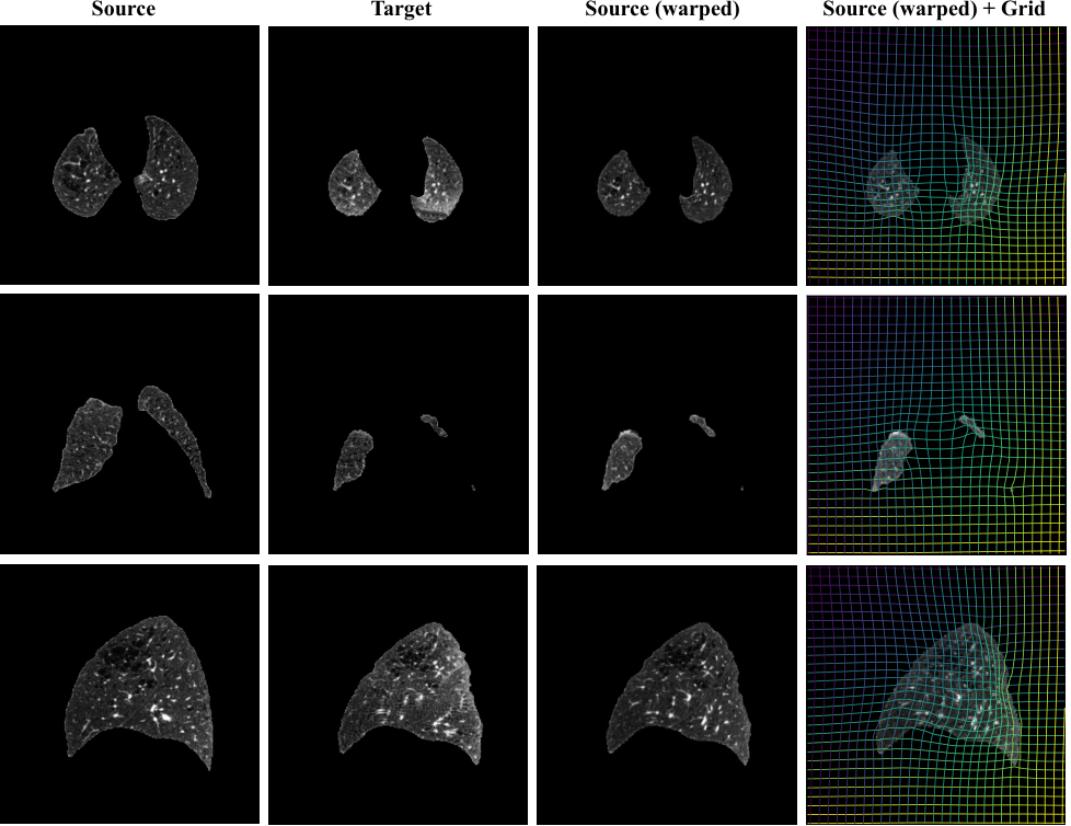
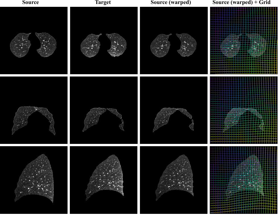
In Fig. 11 and Fig. 12, we show two example registration cases from OAI, Fig. 13 and Fig. 14 show two example registration cases on DirLab, and Fig. 15 and Fig. 16 show two example registration cases on HCP.
In Fig. 17 we show a block diagram of the network structure described in Sec. 4, that is more detailed.




Appendix C Potential negative societal impacts
Image registration results might not be accurate or might even fail for certain image pairs in practice. Hence, careful quality control of the results should be performed when registrations are used for decision-support systems in a medical context.