跳到论文正文
W Papers独立论文阅读器 arXiv:2206.05733 论文正文 计算阅读时间 · 0%
引用这篇论文根据当前论文元数据生成,正式投稿前建议核对。


License: arXiv.org perpetual non-exclusive license
arXiv:2206.05733v2 [cs.LG] 29 Jan 2023

Finite-Time Analysis of Decentralized Single-Timescale
Actor-Critic

Qijun Luo qijunluo@link.cuhk.edu.cn Affiliation: School of Science and Engineering Affiliation: Shenzhen Research Institute of Big Data (SRIBD) Affiliation: The Chinese University of Hong Kong, Shenzhen Affiliation: Shenzhen, China Affiliation: [10pt] Xiao Li lixiao@cuhk.edu.cn Affiliation: School of Data Science Affiliation: Shenzhen Institute of Artificial Intelligence and Robotics for Society (AIRS) Affiliation: The Chinese University of Hong Kong, Shenzhen Affiliation: Shenzhen, China
Abstract

Decentralized Actor-Critic (AC) algorithms have been widely utilized for multi-agent reinforcement learning (MARL) and have achieved remarkable success. Apart from its empirical success, the theoretical convergence property of decentralized AC algorithms is largely unexplored. Most of the existing finite-time convergence results are derived based on either double-loop update or two-timescale step sizes rule, and this is the case even for centralized AC algorithm under a single-agent setting. In practice, the single-timescale update is widely utilized, where actor and critic are updated in an alternating manner with step sizes being of the same order. In this work, we study a decentralized single-timescale AC algorithm. Theoretically, using linear approximation for value and reward estimation, we show that the algorithm has sample complexity of 𝒪~​(ε−2)\tilde{\mathcal{O}}(\varepsilon^{-2}) under Markovian sampling, which matches the optimal complexity with a double-loop implementation (here, 𝒪~\tilde{\mathcal{O}} hides a logarithmic term). When we reduce to the single-agent setting, our result yields new sample complexity for centralized AC using a single-timescale update scheme. The central to establishing our complexity results is the hidden smoothness of the optimal critic variable we revealed. We also provide a local action privacy-preserving version of our algorithm and its analysis. Finally, we conduct experiments to show the superiority of our algorithm over the existing decentralized AC algorithms.

1 Introduction

Multi-agent reinforcement learning (MARL) (Littman 1994; Vinyals et al. 2019) has been successful in various models of multi-agent systems, such as robotics (Lillicrap et al. 2015), autonomous driving (Yu et al. 2019), Go (Silver et al. 2017), etc. MARL has been extensively explored in the past decades; see, e.g., (Lowe et al. 2017; Omidshafiei et al. 2017; Zhang et al. 2021; Son et al. 2019; Espeholt et al. 2018; Rashid et al. 2018). These works either focus on the setting where a central controller is available, or assuming a common reward function for all agents. Among the many cooperative MARL settings, the work (Zhang et al. 2018) proposed the fully decentralized MARL with networked agents. In this setting, each agent maintains a private heterogeneous reward function, and agents can only access local/neighboring information through communicating with its neighboring agents on the network. Then, the objective of all agents is to jointly maximize the average long-term reward through interacting with environment modeled by multi-agent Markov decision process (MDP). They proposed the decentralized Actor-Critic (AC) algorithm to solve this MARL problem, and showed its impressive performance. However, the theoretical convergence properties of such class of decentralized AC algorithms are largely unexplored; see (Zhang et al. 2021) for a comprehensive survey. In this work, our goal is to establish the finite-time convergence results under this fully decentralized MARL setting. We first review some recent progresses on this line of research below.

Related works and motivations. The first fully decentralized AC algorithm with provable convergence guarantee was proposed by (Zhang et al. 2018), and they achieved asymptotic convergence results under two-timescale step sizes, which requires actor’s step sizes to diminish in a faster scale than the critic’s step sizes. The sample complexities of decentralized AC were established recently. In particular, (Chen et al. 2022) and (Hairi et al. 2022) independently proposed two communication efficient decentralized AC algorithms with optimal sample complexity of 𝒪⁡(ε−2​log⁡(ε−1))\mathcal{O}(\varepsilon^{-2}\log(\varepsilon^{-1})) under Markovian sampling scheme. Nevertheless, their analysis are based on double-loop implementation, where each policy optimization step follows a nearly accurate critic optimization step (a.k.a. policy evaluation), i.e., solving the critic optimization subproblem to ε\varepsilon-accuracy. Such a double-loop scheme requires careful tuning of two additional hyper-parameters, which are the batch size and inner loop size. In particular, the batch size and inner loop size need to be of order 𝒪⁡(ε−1)\mathcal{O}(\varepsilon^{-1}) and 𝒪⁡(log⁡(ε−1))\mathcal{O}(\log(\varepsilon^{-1})) in order to achieve their sample complexity results, respectively. In practice, single-loop algorithmic framework is often utilized, where one updates the actor and critic in an alternating manner by performing any constant algorithmic iterations for both subproblems; see, e.g.,  (Schulman et al. 2017; Lowe et al. 2017; Lin et al. 2019; Zhang et al. 2020). The work  (Zeng et al. 2022) proposed a new decentralized AC algorithm based on such a single-loop alternative update. However, they have to adopt two-timescale step sizes rule to ensure convergence, which requires actor’s step sizes to diminish in a faster scale than the critic’s step sizes. Due to the separation of the step sizes, the critic optimization subproblem is solved exactly when the number of iterations tends to ∞\infty. Such a restriction on the step size will slow down the convergence speed of the algorithm. As a consequence, they only obtain sub-optimal sample complexity of 𝒪⁡(ε−52)\mathcal{O}(\varepsilon^{-\frac{5}{2}}). In practice, most algorithms are implemented with single-timescale step sizes rule, where the step sizes for the actor’s and critic’s updates are of the same order. Though there are some theoretical achievements for single-timescale update in other areas such as TDC (Wang et al. 2021) and bi-level optimization (Chen et al. 2021a), similar theoretical understanding under AC setting is largely unexplored.

Indeed, even when reducing to single-agent setting, the convergence property of single-timescale AC algorithm is not well established. The works (Fu et al. 2021; Guo et al. 2021) established the finite-time convergence result under a special single-timescale implementation, where they attained the sample complexity of 𝒪⁡(ε−2)\mathcal{O}(\varepsilon^{-2}). Their analysis is based on an algorithm where the critic optimization step is formulated as a least-square temporal difference (LSTD) at each iteration, which requires to sample the transition tuples for 𝒪~​(ε−1)\tilde{\mathcal{O}}(\varepsilon^{-1}) times to form the data matrix in the LSTD subproblem. Then, they solve the LSTD subproblem in a closed-form fashion by inverting a matrix of large size. Later, (Chen et al. 2021a) obtained the same sample complexity using TD(0) update for critic variables under i.i.d. sampling. Their analysis highly relies on the assumption that the Jacobian of the stationary distribution is Lipschitz continuous, which is not justified in their work.

The above observations motivate us to ask the following question:

Can we establish finite-time convergence result for decentralized AC algorithm with single-timescale step sizes rule?11 1 As convention in (Fu et al. 2021), when we use ”single-timescale”, it means we utilize a single-loop algorithmic framework with single-timescale step sizes rule.

Main contributions. By answering this question positively, we have the following contributions:

  1. ∙\bullet

    We design a decentralized AC algorithm, which employs a single-timescale step sizes rule and adopts Markovian sampling scheme. The proposed algorithm allows communication between agents for every KcK_{c} iterations with KcK_{c} being any integer lies in [1,𝒪⁡(ε−12)][1,\mathcal{O}(\varepsilon^{-\frac{1}{2}})], rather than communicating at each iteration as adopted by previous single-loop decentralized AC algorithms  (Zeng et al. 2022; Zhang et al. 2018).

  2. ∙\bullet

    Using linear approximation for value and reward estimation, we establish the finite-time convergence result for the proposed algorithm under standard assumptions. In particular, we show that the algorithm has a sample complexity of 𝒪~​(ε−2)\tilde{\mathcal{O}}(\varepsilon^{-2}), which matches the optimal complexity up to a logarithmic term. In addition, we show that the logarithmic term hidden in the “𝒪~\tilde{\mathcal{O}}” can be removed under the i.i.d. sampling scheme. These convergence results are valid for all the above mentioned choices for KcK_{c}.

  3. ∙\bullet

    To preserve privacy of local actions, we propose a variant of our algorithm which utilizes noisy local rewards for estimating global rewards. We show that such an algorithm will maintain the optimal sample complexity at the expense of communicating at each iteration.

Our key technical result is to reveal the hidden smoothness of the optimal critic variable, so that we can derive a sufficient descent on the averaged critic’s optimal gap under the single-timescale update. Consequently, we can resort to the classic convergence analysis for alternating optimization algorithms to establish the approximate ascent property of the overall optimization process, which leads to the final sample complexity results. We also designed a Lyapunov function to analyze the descent of the objective function with a single-timescale update under the decentralized setting.

When we reduce to the non-decentralized case, i.e., the single-agent setting, our results yield new sample complexity guarantees for the classic centralized AC algorithm using a single-timescale update scheme.

Discussion on a concurrent work. We note that there is a concurrent work (Olshevsky & Gharesifard 2023) which also analyzes the single-timescale AC algorithm and achieves similar complexity results. Their analysis is based on the small gain theorem, which is different from ours. These two analysis frameworks provide useful insights for the AC algorithm from different perspectives. (Olshevsky & Gharesifard 2023) shows that the coupled expression on the errors of actor and critic can be fit into a non-linear small gain theorem framework, which bounds the actor’s error by desired order. Our analysis reveals the hidden smoothness of the optimal critic variable so that approximate descent on the critic’s objective can be achieved. In addition, (Olshevsky & Gharesifard 2023) considers the single-agent setting while our analysis deals with the more general decentralized setting. Moreover, (Olshevsky & Gharesifard 2023) analyzes the i.i.d. sampling scheme where the single agent is assumed to have access to the transition tuples from the stationary distribution and the discounted state-visitation distribution. By contrast, our setting considers the practical Markovian sampling scheme, where the transition tuples are from the trajectory generated during the update of the agents.

2 Preliminary

In this section, we introduce the problem formulation and the policy gradient theorem, which serves as the preliminary for the analyzed decentralzed AC algorithm.

Suppose there are multiple agents aiming to independently optimize a common global objective, and each agent can communicate with its neighbors through a network. To model the topology, we define the graph as 𝒢=(𝒩,ℰ)\mathcal{G}=(\mathcal{N},\mathcal{E}), where 𝒩\mathcal{N} is the set of nodes with |𝒩|=N|\mathcal{N}|=N and ℰ\mathcal{E} is the set of edges with |ℰ|=E|\mathcal{E}|=E. In the graph, each node represents an agent, and each edge represents a communication link. The interaction between agents follows the networked multi-agent MDP.

2.1 Markov decision process

A networked multi-agent MDP is defined by a tuple (𝒢,𝒮,{𝒜i}i∈[N],𝒫,{ri}i∈[N],γ)(\mathcal{G},\mathcal{S},\{\mathcal{A}^{i}\}_{i\in[N]},\mathcal{P},\{r^{i}\}_{i\in[N]},\gamma). 𝒢\mathcal{G} denotes the communication topology (the graph), 𝒮\mathcal{S} is the finite state space observed by all agents, 𝒜i\mathcal{A}^{i} represents the finite action space of agent ii. Let 𝒜:=𝒜1×⋯×𝒜N\mathcal{A}:=\mathcal{A}^{1}\times\cdots\times\mathcal{A}^{N} denote the joint action space and 𝒫⁡(s′|s,a):𝒮×𝒜×𝒮→[0,1]\mathcal{P}(s^{\prime}|s,a):\mathcal{S}\times\mathcal{A}\times\mathcal{S}\to[0,1] denote the transition probability from any state s∈𝒮s\in\mathcal{S} to any state s′∈𝒮s^{\prime}\in\mathcal{S} for any joint action a∈𝒜a\in\mathcal{A}. ri:𝒮×𝒜→ℝr^{i}:\mathcal{S}\times\mathcal{A}\to\mathbb{R} is the local reward function that determines the reward received by agent ii given transition (s,a)(s,a); γ∈[0,1]\gamma\in[0,1] is the discount factor.

For simplicity, we will use a:=[a1,⋯,aN]a:=[a^{1},\cdots,a^{N}] to denote the joint action, and θ∈ℝN​dθ\theta\in\mathbb{R}^{Nd_{\theta}} to denote concatenation of all actor’s joint parameters of all actors, with θi∈ℝdθ\theta^{i}\in\mathbb{R}^{d_{\theta}}. Here, without loss of generality, we assume that every agent has the same number of parameters for notation brevity. The MDP goes as follows: For a given state ss, each agent make its decision aia^{i} based on its policy ai∼πθi(⋅|s)a^{i}\sim\pi_{\theta^{i}}(\cdot|s). The state transits to the next state s′s^{\prime} based on the joint action of all the agents: s′∼𝒫(⋅|s,a)s^{\prime}\sim\mathcal{P}(\cdot|s,a). Then, each agent will receive its own reward ri​(s,a)r^{i}(s,a). For the notation brevity, we assume that the reward function mapping is deterministic and does not depend on the next state without loss of generality. The stationary distribution induced by the policy πθ\pi_{\theta} and the transition kernel is denoted by μπθ​(s)\mu_{\pi_{\theta}}(s).

Our objective is to find a set of policies that maximize the accumulated discounted mean reward received by agents

θ∗=arg​maxθ⁡J​(θ):=𝔼⁡[∑k=0∞γk​r¯​(sk,ak)].\displaystyle\theta^{*}=\argmax_{\theta}J(\theta):=\mathbb{E}\left[\sum_{k=0}^{\infty}\gamma^{k}\bar{r}(s_{k},a_{k})\right]. (1)

Here, kk represents the time step. r¯​(sk,ak):=1N​∑i=1Nri​(sk,ak)\bar{r}(s_{k},a_{k}):=\frac{1}{N}\sum_{i=1}^{N}r^{i}(s_{k},a_{k}) is the mean reward among agents at time step kk. The randomness of the expectation comes from the initial state distribution μ0​(s)\mu_{0}(s), the transition kernel 𝒫\mathcal{P}, and the stochastic policy πθi(⋅|s)\pi_{\theta^{i}}(\cdot|s).

2.2 Policy gradient Theorem

Under the discounted reward setting, the global state-value function, action-value function, and advantage function for policy set θ\theta, state ss, and action aa, are defined as

Vπθ​(s)\displaystyle V_{\pi_{\theta}}(s) :=𝔼⁡[∑k=0∞γk​r¯​(sk,ak)|s0=s]\displaystyle:=\mathbb{E}\left[\sum_{k=0}^{\infty}\gamma^{k}\bar{r}(s_{k},a_{k})|s_{0}=s\right] (2)
Qπθ​(s,a)\displaystyle Q_{\pi_{\theta}}(s,a) :=𝔼[∑k=0∞γkr¯(sk,ak)|s0=s,a0=a]\displaystyle:=\mathbb{E}\left[\sum_{k=0}^{\infty}\gamma^{k}\bar{r}(s_{k},a_{k})|s_{0}=s,a_{0}=a\right]
Aπθ​(s,a)\displaystyle A_{\pi_{\theta}}(s,a) :=Qπθ​(s,a)−Vπθ​(s).\displaystyle:=Q_{\pi_{\theta}}(s,a)-V_{\pi_{\theta}}(s).

To maximize the objective function defined in (1), the policy gradient (Sutton et al. 2000) can be computed as follow

∇θJ​(θ)=𝔼s∼dπθ,a∼πθ​[11−γ​Aπθ​(s,a)​ψπθ​(s,a)],\displaystyle\nabla_{\theta}J(\theta)=\mathbb{E}_{s\sim d_{\pi_{\theta}},a\sim\pi_{\theta}}\left[\frac{1}{1-\gamma}A_{\pi_{\theta}}(s,a)\psi_{\pi_{\theta}}(s,a)\right],

where dπθ​(s):=(1−γ)​∑k=0∞γk​ℙ​(sk=s)d_{\pi_{\theta}}(s):=(1-\gamma)\sum_{k=0}^{\infty}\gamma^{k}\mathbb{P}(s_{k}=s) is the discounted state visitation distribution under policy πθ\pi_{\theta}, and ψπθ​(s,a):=∇log⁡πθ​(s,a)\psi_{\pi_{\theta}}(s,a):=\nabla\log\pi_{\theta}(s,a) is the score function.

Following the derivation of (Zhang et al. 2018), the policy gradient for each agent under discounted reward setting can be expressed as

∇θiJ​(θ)=𝔼s∼dπθ,a∼πθ​[11−γ​Aπθ​(s,a)​ψπθi​(s,ai)].\displaystyle\nabla_{\theta^{i}}J(\theta)=\mathbb{E}_{s\sim d_{\pi_{\theta}},a\sim\pi_{\theta}}\left[\frac{1}{1-\gamma}A_{\pi_{\theta}}(s,a)\psi_{\pi_{\theta^{i}}}(s,a^{i})\right]. (3)

3 Algorithms

3.1 Decentralized single-timescale Actor-Critic

1:  Initialize: Actor parameter θ0\theta_{0}, critic parameter ω0\omega_{0}, reward estimator parameter λ0\lambda_{0}, initial state s0s_{0}. 2:  for k=0,⋯,K−1k=0,\cdots,K-1 do 3:    Option 1: i.i.d. sampling: 4:    sk∼μθk(s),ak∼πθk(⋅|sk),sk+1∼𝒫(⋅|sk,ak)s_{k}\sim\mu_{\theta_{k}}(s),a_{k}\sim\pi_{\theta_{k}}(\cdot|s_{k}),s_{k+1}\sim\mathcal{P}(\cdot|s_{k},a_{k}). 5:    Option 2: Markovian sampling: 6:    ak∼πθk(⋅|sk),sk+1∼𝒫(⋅|sk,ak)a_{k}\sim\pi_{\theta_{k}}(\cdot|s_{k}),s_{k+1}\sim\mathcal{P}(\cdot|s_{k},a_{k}). 7:     8:    Periodical consensus: Compute ω~ki\tilde{\omega}_{k}^{i} and λ~ki\tilde{\lambda}_{k}^{i} by (4) and (7). 9:     10:    for i=0,⋯,Ni=0,\cdots,N in parallel do 11:     Reward estimator update: update λk+1i\lambda_{k+1}^{i} by (8). 12:     Critic update: Update ωk+1i\omega_{k+1}^{i} by (5). 13:     Actor update: Update θk+1i\theta_{k+1}^{i} by (6). 14:    end for 15:  end for
Algorithm 1 Decentralized single-timescale AC (reward estimator version)

We introduce the decentralized single-timescale AC algorithm; see Algorithm 1. In the remaining parts of this section, we will explain the updates in the algorithm in details.

In fully-decentralized MARL, each agent can only observe its local reward and action, while trying to maximize the global reward (mean reward) defined in (1). The decentralized AC algorithm solves the problem by updating actor and critic variables alternatively on an online trajectory. Specifically, we have NN pairs of actor and critic. In order to maximize J⁡(θ)J(\theta), each critic tries to estimate the global state-value function Vπθ​(s)V_{\pi_{\theta}}(s) defined in (2). Then, each actor updates its policy parameter based on approximated policy gradient. We now provide more details about the algorithm.

Critics’ update. We will use ωi∈ℝdω\omega^{i}\in\mathbb{R}^{d_{\omega}} to denote the it​hi_{th} critic’s parameter and ω¯:=1N​∑i=1Nωi\bar{\omega}:=\frac{1}{N}\sum_{i=1}^{N}\omega^{i} to represent the averaged parameter of critic. Each critic approximates the global value function as Vπθ​(s)≈V^ωi​(s)V_{\pi_{\theta}}(s)\approx\hat{V}_{\omega^{i}}(s).

The critic’s approximation error can be categorized into two parts, namely, the consensus error 1N​∑i=1N‖ωi−ω¯‖,\frac{1}{N}\sum_{i=1}^{N}\|\omega^{i}-\bar{\omega}\|, which measures how close the critics’ parameters are; and the approximation error ‖ω¯−ω∗​(θ)‖,\|\bar{\omega}-\omega^{*}(\theta)\|, which measures the approximation quality of averaged critic.

In order for critics to reach consensus, each critic exchanges its parameters with neighbors and perform the following update

ω~ki={∑j=1NWi​j​ωkjif​kmodKc=0ωkiotherwise.\displaystyle\tilde{\omega}_{k}^{i}=\begin{cases}\sum_{j=1}^{N}W^{ij}\omega_{k}^{j}\quad&\text{if}~k\hskip-5.69046pt\mod K_{c}=0\\ \omega_{k}^{i}\quad&\text{otherwise}.\end{cases} (4)

Here, KcK_{c} denotes the consensus frequency. The communication matrix W∈ℝn×nW\in\mathbb{R}^{n\times n} is usually determined artificially in practice and can be sparse, which means that the number of neighbors for each agent is much fewer than the total number of agents. Thus, the cost for each consensus step is usually much lower than a full synchronization over the network. The detailed requirements of matrix WW will be discussed in Assumption 5.

To reduce the approximation error, we will perform the local TD(0) update (Tsitsiklis & Van Roy 1997) as

ωk+1i\displaystyle\omega_{k+1}^{i} =ΠRω​(ω~ki+βk​gci​(ξk,ωki)),\displaystyle=\Pi_{R_{\omega}}(\tilde{\omega}_{k}^{i}+\beta_{k}g_{c}^{i}(\xi_{k},\omega_{k}^{i})), (5)

where ξ:=(s,a,s′)\xi:=(s,a,s^{\prime}) represents a transition tuple, gci(ξ,ω):=δi(ξ,ω)∇V^ω(s)g_{c}^{i}(\xi,\omega):=\delta^{i}(\xi,\omega)\nabla\hat{V}_{\omega}(s) is the update direction, δi​(ξ,ω):=ri​(s,a)+γ​V^ω​(s′)−V^ω​(s)\delta^{i}(\xi,\omega):=r^{i}(s,a)+\gamma\hat{V}_{\omega}(s^{\prime})-\hat{V}_{\omega}(s) is the local temporal difference error (TD-error). βk\beta_{k} is the step size for critic at iteration kk. ΠRω\Pi_{R_{\omega}} projects the parameter into a ball of radius of RωR_{\omega} containing the optimal solution, which will be explained when discussing Assumptions 1 and 2.

Actors’ update. We will use stochastic gradient ascent to update the policy’s parameter, which is calculated based on policy gradient theorem in (3). The advantage function Aπθ​(s,a)A_{\pi_{\theta}}(s,a) can be estimated by

δ⁡(ξ,θ):=r¯​(s,a)+γ​Vπθ​(s′)−Vπθ​(s),\displaystyle\delta(\xi,\theta):=\bar{r}(s,a)+\gamma V_{\pi_{\theta}}(s^{\prime})-V_{\pi_{\theta}}(s),

with aa sampled from πθ(⋅|s)\pi_{\theta}(\cdot|s). However, to preserve the privacy of each agents, the local reward cannot be shared to other agents under the fully decentralized setting. Thus, the averaged reward r¯​(sk,ak)\bar{r}(s_{k},a_{k}) is not directly attainable. To this end, we adopt the strategy proposed in (Zhang et al. 2018) to approximate the averaged reward. In particular, each agent ii will have a local reward estimator with parameter λi∈ℝdλ\lambda^{i}\in\mathbb{R}^{d_{\lambda}}, which estimates the global averaged reward as r¯​(sk,ak)≈r^λi​(sk,ak)\bar{r}(s_{k},a_{k})\approx\hat{r}_{\lambda^{i}}(s_{k},a_{k}).

Thus, the update of the it​hi_{th} actor is given by

θk+1i=θki+αk​δ^​(ξk,ωk+1i,λk+1i)​ψπθki​(sk,aki),\displaystyle\theta_{k+1}^{i}=\theta_{k}^{i}+\alpha_{k}\hat{\delta}(\xi_{k},\omega_{k+1}^{i},\lambda_{k+1}^{i})\psi_{\pi_{\theta_{k}^{i}}}(s_{k},a_{k}^{i}), (6)

where δ^​(ξ,ω,λ):=r^λ​(s,a)+γ​V^ω​(s′)−V^ω​(s)\hat{\delta}(\xi,\omega,\lambda):=\hat{r}_{\lambda}(s,a)+\gamma\hat{V}_{\omega}(s^{\prime})-\hat{V}_{\omega}(s) is the approximated advantage function. αk\alpha_{k} is the step size for actor’s update at iteration kk.

Reward estimators’ update. Similar to critic, each reward estimator’s approximation error can be decomposed into consensus error and the approximation error.

For each local reward estimator, we perform the consensus step to minimize the consensus error as

λ~ki={∑j=1NWi​j​λkjif​kmodKc=0λkiotherwise.\displaystyle\tilde{\lambda}_{k}^{i}=\begin{cases}\sum_{j=1}^{N}W^{ij}\lambda_{k}^{j}\quad&\text{if}~k\hskip-5.69046pt\mod K_{c}=0\\ \lambda_{k}^{i}\quad&\text{otherwise}.\end{cases} (7)

To reduce the approximation error, we perform a local update of stochastic gradient descent.

λk+1i\displaystyle\lambda_{k+1}^{i} =ΠRλ​(λ~ki+ηk​gri​(ξk,λki)),\displaystyle=\Pi_{R_{\lambda}}(\tilde{\lambda}_{k}^{i}+\eta_{k}g_{r}^{i}(\xi_{k},\lambda_{k}^{i})), (8)

where gri(ξ,λ):=(ri(s,a)−r^λ(s,a))∇r^λ(s,a)g_{r}^{i}(\xi,\lambda):=(r^{i}(s,a)-\hat{r}_{\lambda}(s,a))\nabla\hat{r}_{\lambda}(s,a) is the update direction. ηk\eta_{k} is the step size for reward estimator at iteration kk. Note the calculation of gri​(ξ,λ)g_{r}^{i}(\xi,\lambda) does not depend on the next state s′s^{\prime}; we use ξ\xi in (8) just for notation brevity. Similar to critic’s update, ΠRλ\Pi_{R_{\lambda}} projects the parameter into a ball of radius of RλR_{\lambda} containing the optimal solution.

In our Algorithm 1, we will use the same order for αk\alpha_{k}, βk\beta_{k}, and ηk\eta_{k} and hence, our algorithm is in single-timescale.

Linear approximation for analysis. In our analysis, we will use linear approximation for both critic and reward estimator variables, i.e. V^ω​(s):=ϕ​(s)T​ω\hat{V}_{\omega}(s):=\phi(s)^{T}\omega; r^λ​(s,a):=φ​(s,a)T​λ\hat{r}_{\lambda}(s,a):=\varphi(s,a)^{T}\lambda, where ϕ⁡(s):𝒮→ℝdω\phi(s):\mathcal{S}\to\mathbb{R}^{d_{\omega}} and φ⁡(s,a):𝒮×𝒜→ℝdλ\varphi(s,a):\mathcal{S}\times\mathcal{A}\to\mathbb{R}^{d_{\lambda}} are two feature mappings, whose property will be specified in the discussion of Assumption 1.

Remarks on sampling scheme. Acquiring unbiased stochastic gradients for critic and actor variables requires sampling from μπθ\mu_{\pi_{\theta}} and dπθd_{\pi_{\theta}}, respectively. However, in practical implementations, states are usually collected from an online trajectory (Markovian sampling), whose distribution is generally different from μπθ\mu_{\pi_{\theta}} and dπθd_{\pi_{\theta}}. Such a distribution mismatch will inevitably cause biases during the update of critic and actor variables. One has to bound the corresponding error terms when analyzing the algorithm.

1:  Initialize: Actor parameter θ0\theta_{0}, critic parameter ω0\omega_{0}, initial state s0s_{0}. 2:  for k=0,⋯,K−1k=0,\cdots,K-1 do 3:    Option 1: i.i.d. sampling: 4:    sk∼μθk(s),ak∼πθk(⋅|sk),sk+1∼𝒫(⋅|sk,ak)s_{k}\sim\mu_{\theta_{k}}(s),a_{k}\sim\pi_{\theta_{k}}(\cdot|s_{k}),s_{k+1}\sim\mathcal{P}(\cdot|s_{k},a_{k}). 5:    Option 2: Markovian sampling: 6:    ak∼πθk(⋅|sk),sk+1∼𝒫(⋅|sk,ak)a_{k}\sim\pi_{\theta_{k}}(\cdot|s_{k}),s_{k+1}\sim\mathcal{P}(\cdot|s_{k},a_{k}). 7:     8:    Periodical consensus: Compute ω~ki\tilde{\omega}_{k}^{i} by (4). 9:     10:    for i=0,⋯,Ni=0,\cdots,N in parallel do 11:     Global reward estimation: estimate r¯k​(sk,ak)\bar{r}_{k}(s_{k},a_{k}) by (9). 12:     Critic update: Update ωk+1i\omega_{k+1}^{i} by (5). 13:     Actor update: Update θk+1i\theta_{k+1}^{i} by (10). 14:    end for 15:  end for
Algorithm 2 Decentralized single-timescale AC (noisy reward version)

3.2 Variant for preserving local action

Note that in Algorithm 1, the reward estimators need the knowledge of joint actions in order to estimate the global rewards. Inspired by (Chen et al. 2022), we further propose a variant of Algorithm 1 to preserve the privacy of local actions. It estimates the global rewards by communicating noisy local rewards. As a trade-off, the approach requires 𝒪⁡(log⁡(ε−1))\mathcal{O}(\log(\varepsilon^{-1})) communication rounds for each iteration; see Algorithm 2.

Let rkir_{k}^{i} represents rki​(sk,ak)r_{k}^{i}(s_{k},a_{k}) for brevity. The reward estimation process goes as follow: for each agent ii, we first produce a noisy local reward r~ki=rki​(1+z)\tilde{r}_{k}^{i}=r_{k}^{i}(1+z), with z∼𝒩⁡(0,σ2)z\sim\mathcal{N}(0,\sigma^{2}). Thus, the noise level is controlled by the variance σ2\sigma^{2}, which is chosen artificially. When the noise level σ2\sigma^{2} increases, the local reward’s privacy will be strengthen. In the meantime, the variance of the estimated global reward will increase. To estimate the global reward, each agent ii first initialize the estimation as r~k,0i=r~ki\tilde{r}_{k,0}^{i}=\tilde{r}_{k}^{i}. Then, each agent ii perform the following consensus step for KrK_{r} times, i.e.

r~k,l+1i=∑j=1NWi​jr~k,li,l=0,1,⋯,Kr−1.\displaystyle\tilde{r}_{k,l+1}^{i}=\sum_{j=1}^{N}W^{ij}\tilde{r}_{k,l}^{i},\quad l=0,1,\cdots,K_{r}-1. (9)

The reward r~k,Kri\tilde{r}_{k,K_{r}}^{i} will be used for estimating the global reward for agent ii at kt​hk_{th} iteration. As we will see, the error |r~t,l+1i−1N​∑i=1Nr~ki||\tilde{r}_{t,l+1}^{i}-\frac{1}{N}\sum_{i=1}^{N}\tilde{r}_{k}^{i}| will converge to 0 linearly. Hence, to reduce the error to ε\varepsilon, we need Kr=𝒪⁡(log⁡(ε−1))K_{r}=\mathcal{O}(\log(\varepsilon^{-1})) rounds of communications for each iteration. Based on the estimated global reward, the it​hi_{th} actor’s update is given by

θk+1i=θki+αk​(r~k,Kri+γ​V^ωi​(s′)−V^ωi​(s))​ψπθki​(sk,aki).\displaystyle\theta_{k+1}^{i}=\theta_{k}^{i}+\alpha_{k}(\tilde{r}_{k,K_{r}}^{i}+\gamma\hat{V}_{\omega^{i}}(s^{\prime})-\hat{V}_{\omega^{i}}(s))\psi_{\pi_{\theta_{k}^{i}}}(s_{k},a_{k}^{i}). (10)

4 Main results

In this section, we first introduce the technical assumptions used for our analysis, which are standard in the literature. Then, we present the convergence results for both actor and critic variables.

4.1 Assumptions

Assumption 1 (boundedness of rewards and feature vectors).

The local rewards are uniformly bounded, i.e., there exists a positive constant rmaxr_{\max} such that for all feasible (s,a)(s,a) and i∈[N]i\in[N], we have |ri​(s,a)|≤rmax|\,r^{i}(s,a)\,|\leq r_{\max}. The norm of feature vectors are bounded such that for all s∈𝒮,a∈𝒜s\in\mathcal{S},\ a\in\mathcal{A}, ‖ϕ⁡(s)‖≤1,‖φ⁡(s,a)‖≤1\|\phi(s)\|\leq 1,\|\varphi(s,a)\|\leq 1.22 2 Through out the paper, we will use ∥⋅∥\|\cdot\| to represent the Euclidean norm for vectors and Frobenius norm for matrices.

Assumption 1 is standard and commonly adopted; see, e.g.,  (Bhandari et al. 2018; Xu et al. 2020; Zeng et al. 2022; Shen et al. 2020; Qiu et al. 2019). This assumption can be achieved via normalizing the feature vectors.

Assumption 2 (sufficient exploration).

There exists two positive constants λϕ,λφ\lambda_{\phi},\lambda_{\varphi} such that for all policy πθ\pi_{\theta}, the following two matrices are negative definite

Aθ,ϕ\displaystyle A_{\theta,\phi} :=𝔼s∼μθ​(s)​[ϕ⁡(s)​(γ​ϕ​(s′)T−ϕ​(s)T)]\displaystyle:=\mathbb{E}_{s\sim\mu_{\theta}(s)}[\phi(s)(\gamma\phi(s^{\prime})^{T}-\phi(s)^{T})]
Aθ,φ\displaystyle A_{\theta,\varphi} :=𝔼s∼μθ(s),a∼πθ(⋅|s)[−φ(s,a)φ(s,a)T],\displaystyle:=\mathbb{E}_{s\sim\mu_{\theta}(s),a\sim\pi_{\theta}(\cdot|s)}[-\varphi(s,a)\varphi(s,a)^{T}],

with λmax​(Aθ,ϕ)≤λϕ,λmax​(Aθ,φ)≤λφ\lambda_{\max}(A_{\theta,\phi})\leq\lambda_{\phi},\lambda_{\max}(A_{\theta,\varphi})\leq\lambda_{\varphi}, where λmax​(⋅)\lambda_{\max}(\cdot) represents the largest eigenvalue.

The Assumption 2 characterizes a strong convexity-like property of critic and reward estimator’s objective function, and thereby ensures sufficient decrease of the estimation error for each update. It will be satisfied when infθ,s,aπθ​(a|s)≥c\inf_{\theta,s,a}\pi_{\theta}(a|s)\geq c for all policy πθ,s∈𝒮,a∈𝒜\pi_{\theta},s\in\mathcal{S},a\in\mathcal{A} with cc being positive. Thus, it can be understood as an exploration assumption on policy πθ\pi_{\theta}. (see Proposition 3.1 of (Olshevsky & Gharesifard 2023) for more detail). This assumption is widely seen in analysis of AC algorithms; see, e.g. (Shen et al. 2020; Xu & Liang 2021; Zeng et al. 2022). Together with Assumption 1, we can show that ‖ω∗​(θ)‖≤Rω:=rmaxλϕ\|\omega^{*}(\theta)\|\leq R_{\omega}:=\frac{r_{\max}}{\lambda_{\phi}}, ‖λ∗​(θ)‖≤Rλ:=rmaxλφ\|\lambda^{*}(\theta)\|\leq R_{\lambda}:=\frac{r_{\max}}{\lambda_{\varphi}}, which justifies the projection step. In practice, one can estimate RωR_{\omega} and RλR_{\lambda} online; see Section 8.2 of (Bhandari et al. 2018) for one approach. We provide more details for the projection in Appendix C.

Assumption 3 (Lipschitz properties of policy).

There exists constants Cψ,Lψ,LπC_{\psi},L_{\psi},L_{\pi} such that for all policy parameter θ,θ′\theta,\theta^{\prime}, s∈𝒮s\in\mathcal{S} and a∈𝒜a\in\mathcal{A}, we have (1).|πθ​(a|s)−πθ′​(a|s)|≤Lπ​‖θ−θ′‖;(2).‖ψθ​(s,a)−ψθ′​(s,a)‖≤Lψ​‖θ−θ′‖;(3).‖ψθ​(s,a)‖≤Cψ(1).~|\pi_{\theta}(a|s)-\pi_{\theta^{\prime}}(a|s)|\leq L_{\pi}\|\theta-\theta^{\prime}\|;(2).~\|\psi_{\theta}(s,a)-\psi_{\theta^{\prime}}(s,a)\|\leq L_{\psi}\|\theta-\theta^{\prime}\|;(3).~\|\psi_{\theta}(s,a)\|\leq C_{\psi}.

Assumption 3 is common for analyzing policy-based algorithms; see, e.g., (Xu et al. 2019; Wu et al. 2020; Hairi et al. 2022). The assumption implies the smoothness of objective function J⁡(θ)J(\theta). It holds for policy classes such as tabular softmax policy (Agarwal et al. 2020), Gaussian policy (Doya 2000), and Boltzmann policy (Konda & Borkar 1999).

Assumption 4 (mixing of Markov chain).

There exists constants κ>0\kappa>0 and ρ∈(0,1)\rho\in(0,1) such that

sups∈𝒮dT​V(ℙ(sk∈⋅|s0=s,πθ),μθ)≤κρk,∀k.\displaystyle\sup_{s\in\mathcal{S}}d_{{TV}}\ (\mathbb{P}(s_{k}\in\cdot|s_{0}=s,\pi_{\theta}),\mu_{\theta})\leq\kappa\rho^{k},\ \forall k.

Assumption 4 is a standard assumption; see, e.g. (Bhandari et al. 2018; Wu et al. 2020; Xu et al. 2019). The assumption always holds for irreducible and aperiodic Markov chain. It ensures the geometric convergence of state to the stationary distribution.

Assumption 5 (doubly stochastic weight matrix).

The communication matrix WW is doubly stochastic, i.e. each column/row sum up to 1. Moreover, the second largest singular value ν\nu is smaller than 1.

Assumption 5 is a common assumption in decentralized optimization and multi-agent reinforcement learning; see, e.g.,  (Sun et al. 2020; Chen et al. 2021b; Chen et al. 2022). It ensures the convergence of consensus error for critic and reward estimator variables.

4.2 Sample complexity for Algorithm 1

Theorem 1.

Suppose Assumptions 1-5 hold. Consider the update of Algorithm 1 under Markovian sampling. Let αk=α¯K\alpha_{k}=\frac{\bar{\alpha}}{\sqrt{K}} for some positive constant α¯\bar{\alpha}, βk=C92​λϕ​αk\beta_{k}=\frac{C_{9}}{2\lambda_{\phi}}\alpha_{k}, and ηk=C102​λφ​αk\eta_{k}=\frac{C_{10}}{2\lambda_{\varphi}}\alpha_{k} and Kc≤𝒪⁡(K1/4)K_{c}\leq\mathcal{O}({K^{1/4}}), where KK is the total number of iterations. Then, we have

1K​∑k=1K∑i=1N𝔼⁡[‖ωki−ω∗​(θk)‖2]≤𝒪⁡(log2⁡KK)\displaystyle\frac{1}{K}\sum_{k=1}^{K}\sum_{i=1}^{N}\mathbb{E}\left[\left\|\omega_{k}^{i}-\omega^{*}(\theta_{k})\right\|^{2}\right]\leq\mathcal{O}\left(\frac{\log^{2}K}{\sqrt{K}}\right)
1K​∑k=1K∑i=1N𝔼⁡[‖∇θiJ​(θk)‖2]≤𝒪⁡(log2⁡KK)+𝒪⁡(εa​p​p+εs​p),\displaystyle\frac{1}{K}\sum_{k=1}^{K}\sum_{i=1}^{N}\mathbb{E}\left[\left\|\nabla_{\theta^{i}}{J}(\theta_{k})\right\|^{2}\right]\leq\mathcal{O}\left(\frac{\log^{2}K}{\sqrt{K}}\right)+\mathcal{O}\left(\varepsilon_{app}+\varepsilon_{sp}\right), (11)

where C9,C10C_{9},C_{10} are positive constants defined in proof.

The proof of Theorem 1 can be found in Appendix D.1. It establishes the iteration complexity of 𝒪⁡(log2⁡K/K)\mathcal{O}({\log^{2}K}/{\sqrt{K}}), or equivalently, sample complexity of 𝒪~​(ε−2)\tilde{\mathcal{O}}(\varepsilon^{-2}) for Algorithm 1. Note that actors, critics, and reward estimators use the step size of the same order. The rate matches the state-of-the-art sample complexity of decentralized AC algorithms up to a logarithmic term, which are implemented in double-loop fashion (Hairi et al. 2022; Chen et al. 2022). The approximation error is defined as

εa​p​p:=maxθ,a⁡𝔼s∼μθ​[|Vπθ​(s)−V^ω∗​(θ)​(s)|2+|r¯​(s,a)−r^λ∗​(θ)​(s,a)|2].\displaystyle\varepsilon_{app}:=\max_{\theta,a}{\mathbb{E}_{s\sim\mu_{\theta}}\left[\left|V_{\pi_{\theta}}(s)-\hat{V}_{\omega^{*}(\theta)}(s)\right|^{2}+\left|\bar{r}(s,a)-\hat{r}_{\lambda^{*}(\theta)}(s,a)\right|^{2}\right]}. (12)

The error εa​p​p\varepsilon_{app} captures the approximation power of critic and reward estimator. When using function approximation, such an error is inevitable. Similar terms also appear in the literature (see, e.g., (Xu et al. 2020; Agarwal et al. 2020; Qiu et al. 2019)). εa​p​p\varepsilon_{app} becomes zero in tabular case. The error εs​p\varepsilon_{sp} represents the mismatch between the discounted state visitation distribution dπθd_{\pi_{\theta}} and stationary distribution μπθ\mu_{\pi_{\theta}}. It is defined as

εs​p:=4​Cθ2​(logρ⁡κ−1+1ρ)2​(1−γ)2.\varepsilon_{sp}:=4C_{\theta}^{2}\left(\log_{\rho}\kappa^{-1}+\frac{1}{\rho}\right)^{2}\left(1-\gamma\right)^{2}.

By policy gradient theorem (3), the states should be sampled from discounted state visitation distribution in order to attain unbiased estimation of policy gradient. Nevertheless, the state distribution converges to stationary distribution μπθ\mu_{\pi_{\theta}} due to Markov chain’s mixing, which inevitably introduces the sampling error εs​p\varepsilon_{sp}. Similar terms also appear in (Zeng et al. 2022; Shen et al. 2020). When γ\gamma is close to 1, the error becomes small. This is because dπθd_{\pi_{\theta}} approaches to μπθ\mu_{\pi_{\theta}} when γ\gamma goes to 1. In the literature, some works assume that sampling from dπθd_{\pi_{\theta}} is permitted, thus eliminate this error; see, e.g., (Chen et al. 2021a).

Complexity result under i.i.d. sampling. Under the i.i.d. sampling scheme, state can be directly sampled from μπθ\mu_{\pi_{\theta}} and dπθd_{\pi_{\theta}}. In this case, the logarithmic term caused by the Markovian mixing time, and the error εs​p\varepsilon_{sp} caused by the distribution mismatch, can be avoided. In this sense, one can attain the iteration complexity of 𝒪⁡(1/K)\mathcal{O}(1/\sqrt{K}), or equivalently, sample complexity of 𝒪⁡(ε−2)\mathcal{O}(\varepsilon^{-2}).

4.3 Sample complexity for Algorithm 2

Theorem 2.

Suppose Assumptions 1-5 hold. Consider the update of Algorithm 2 under Markovian sampling. Let αk=α¯K\alpha_{k}=\frac{\bar{\alpha}}{\sqrt{K}} for some positive constant α¯\bar{\alpha} and βk=C92​λϕ​αk\beta_{k}=\frac{C_{9}}{2\lambda_{\phi}}\alpha_{k}, Kr=log⁡(K1/2)K_{r}=\log(K^{1/2}), Kc≤𝒪⁡(K1/4)K_{c}\leq\mathcal{O}({K^{1/4}}), where KK is the total number of iterations. Then, we have

1K​∑k=1K∑i=1N𝔼⁡[‖ωki−ω∗​(θk)‖2]≤𝒪⁡(log2⁡KK)\displaystyle\frac{1}{K}\sum_{k=1}^{K}\sum_{i=1}^{N}\mathbb{E}\left[\|\omega_{k}^{i}-\omega^{*}(\theta_{k})\|^{2}\right]\leq\mathcal{O}\left(\frac{\log^{2}K}{\sqrt{K}}\right)
1K​∑k=1K∑i=1N𝔼⁡[‖∇θiJ​(θk)‖2]≤𝒪⁡(log2⁡KK)+𝒪⁡(εa​p​pc+εs​p),\displaystyle\frac{1}{K}\sum_{k=1}^{K}\sum_{i=1}^{N}\mathbb{E}\left[\|\nabla_{\theta^{i}}{J}(\theta_{k})\|^{2}\right]\leq\mathcal{O}\left(\frac{\log^{2}K}{\sqrt{K}}\right)+\mathcal{O}(\varepsilon_{app}^{c}+\varepsilon_{sp}), (13)

where the constants are defined in proof.

The proof of Theorem 2 can be found in Appendix D.2. It establishes the sample complexity of 𝒪~​(ε−2)\tilde{\mathcal{O}}(\varepsilon^{-2}) for Algorithm 2. The εa​p​pc\varepsilon_{app}^{c} captures the approximation error of the critic variables, which is defined as

εa​p​pc:=maxθ⁡𝔼s∼μθ​[|Vπθ​(s)−V^ω∗​(θ)​(s)|2].\varepsilon_{app}^{c}:=\max_{\theta}\mathbb{E}_{s\sim\mu_{\theta}}\left[\left|V_{\pi_{\theta}}(s)-\hat{V}_{\omega^{*}(\theta)}(s)\right|^{2}\right].

The Algorithm 2 preserves the privacy of local actions and requires less parameters than Algorithm 1 since there is no reward estimator. The cost is that it needs to communicate 𝒪⁡(log⁡(ε−1))\mathcal{O}(\log(\varepsilon^{-1})) times for each iteration.

4.4 Proof sketch

We present the main elements for the proof of Theorem 1, which helps in understanding the difference between classical two-timescale/double-loop analysis and our single-timescale analysis. The proof of Theorem 2 follows the similar framework.

Under Markovian sampling, it is possible to show the following inequality, which characterizes the ascent of the objective.

𝔼⁡[J⁡(θk+1)]−J⁡(θk)\displaystyle\mathbb{E}[J(\theta_{k+1})]-J(\theta_{k}) ≥∑i=1N[αk2𝔼∥∇θiJ(θk)∥2+αk2𝔼∥gai(ξk,ωk+1i,λk+1i)∥2\displaystyle\geq\sum_{i=1}^{N}\left[\frac{\alpha_{k}}{2}\mathbb{E}\|\nabla_{\theta^{i}}J(\theta_{k})\|^{2}+\frac{\alpha_{k}}{2}\mathbb{E}\|g_{a}^{i}(\xi_{k},\omega_{k+1}^{i},\lambda_{k+1}^{i})\|^{2}\right.
−8Cψ2αk𝔼∥ω∗(θk)−ωk+1i∥2−4Cψ2αk𝔼∥λ∗(θk)−λk+1i∥2]\displaystyle\quad\left.-8C_{\psi}^{2}\alpha_{k}\mathbb{E}\|\omega^{*}(\theta_{k})-\omega_{k+1}^{i}\|^{2}-4C_{\psi}^{2}\alpha_{k}\mathbb{E}\|\lambda^{*}(\theta_{k})-\lambda_{k+1}^{i}\|^{2}\vphantom{\frac{\alpha_{k}}{2}}\right]
−𝒪⁡(log2⁡(K)​αk2)−𝒪⁡((εa​p​p+εs​p)​αk).\displaystyle\quad-\mathcal{O}(\log^{2}(K)\alpha_{k}^{2})-\mathcal{O}((\varepsilon_{app}+\varepsilon_{sp})\alpha_{k}). (14)

To analyze the errors of critic ‖ω∗​(θk)−ωk+1i‖2\|\omega^{*}(\theta_{k})-\omega_{k+1}^{i}\|^{2} and reward estimator ‖λ∗​(θk)−λk+1i‖2\|\lambda^{*}(\theta_{k})-\lambda_{k+1}^{i}\|^{2}, the two-timescale analysis requires 𝒪⁡(αk)<min⁡{𝒪⁡(βk),𝒪⁡(ηk)}\mathcal{O}(\alpha_{k})<\min\{\mathcal{O}(\beta_{k}),\mathcal{O}(\eta_{k})\} in order for these two errors to converge. The double-loop approach runs lower-level update for 𝒪⁡(log⁡(ε−1))\mathcal{O}(\log(\varepsilon^{-1})) times with batch size 𝒪⁡(ε−1)\mathcal{O}(\varepsilon^{-1}) to drive these errors below ε\varepsilon and hence, they cannot allow inner loop size and bath size to be 𝒪⁡(1)\mathcal{O}(1) simultaneously. To obtain the convergence result for single-timescale update, the idea is to further upper bound these two lower-level errors by the quantity 𝒪⁡(αk​𝔼​‖gai​(ξk,ωk+1i,λk+1i)‖2)\mathcal{O}(\alpha_{k}\mathbb{E}\|g_{a}^{i}(\xi_{k},\omega_{k+1}^{i},\lambda_{k+1}^{i})\|^{2}) (through a series of derivations), and then eliminate these errors by the ascent term αk2​𝔼​‖gai​(ξk,ωk+1i,λk+1i)‖2\frac{\alpha_{k}}{2}\mathbb{E}\|g_{a}^{i}(\xi_{k},\omega_{k+1}^{i},\lambda_{k+1}^{i})\|^{2}.

We mainly focus on the analysis of critic’s error through the proof sketch. The analysis for reward estimator’s error follows similar procedure. We start by decomposing the error of critic as

∑i=1N‖ωk+1i−ω∗​(θk)‖2=∑i=1N(‖ωk+1i−ω¯k+1‖2+‖ω¯k+1−ω∗​(θk)‖2).\displaystyle\sum_{i=1}^{N}\|\omega_{k+1}^{i}-\omega^{*}(\theta_{k})\|^{2}=\sum_{i=1}^{N}(\|\omega_{k+1}^{i}-\bar{\omega}_{k+1}\|^{2}+\|\bar{\omega}_{k+1}-\omega^{*}(\theta_{k})\|^{2}). (15)

The first term represents the consensus error, which can be bounded by the next lemma.

Lemma 1.

Suppose Assumptions 1 and 5 hold. Consider the sequence {ωki}\{\omega_{k}^{i}\} generated by Algorithm 1, then the following holds

‖Q​𝝎k+1‖≤νkKc−1​‖𝝎0‖+4​N​Cδ​∑t=0kνk−tKc−1​βt,\displaystyle\|Q\bm{\omega}_{k+1}\|\leq\nu^{\frac{k}{K_{c}}-1}\|\bm{\omega}_{0}\|+4\sqrt{N}C_{\delta}\sum_{t=0}^{k}\nu^{\frac{k-t}{K_{c}}-1}\beta_{t},

where 𝛚k:=[ωk1,⋯,ωkN]T,Q:=I−1N​11T\bm{\omega}_{k}:=[\omega_{k}^{1},\cdots,\omega_{k}^{N}]^{T},Q:=I-\frac{1}{N}\textbf{1}\textbf{1}^{T}, ν∈(0,1)\nu\in(0,1) is the second largest singular value of WW.

Based on Lemma 1 and follow the step size rule of Theorem 1, it is possible to show ‖Q​𝝎k+1‖2=∑i=1N‖ωk+1i−ω¯k+1‖2=𝒪⁡(Kc2​βk2)\|Q\bm{\omega}_{k+1}\|^{2}=\sum_{i=1}^{N}\|\omega_{k+1}^{i}-\bar{\omega}_{k+1}\|^{2}=\mathcal{O}(K_{c}^{2}\beta_{k}^{2}). Let Kc=𝒪⁡(βk−12)K_{c}=\mathcal{O}(\beta_{k}^{-\frac{1}{2}}), we have ‖Q​𝝎k+1‖2=𝒪⁡(βk)\|Q\bm{\omega}_{k+1}\|^{2}=\mathcal{O}(\beta_{k}), which maintains the optimal rate.

To analyze the second term in (15), we first construct the following Lyapunov function

𝕍k:=−J⁡(θk)+‖ω¯k−ω∗​(θk)‖2+‖λ¯k−λ∗​(θk)‖2.\displaystyle\mathbb{V}_{k}:=-J(\theta_{k})+\|\bar{\omega}_{k}-\omega^{*}(\theta_{k})\|^{2}+\|\bar{\lambda}_{k}-\lambda^{*}(\theta_{k})\|^{2}. (16)

Then, it remains to derive an approximate descent property of the term ‖ω¯k−ω∗​(θk)‖2\|\bar{\omega}_{k}-\omega^{*}(\theta_{k})\|^{2} in (16). Towards that end, our key step lies in establishing the smoothness of the optimal critic variables shown in the next lemma.

Lemma 2 (Smoothness of optimal critic).

Suppose Assumptions 1-3 hold, under the update of Algorithm 1, there exists a positive constant Lω,2L_{\omega,2} such that for any policy parameter θ1,θ2\theta_{1},\theta_{2}, it holds that

‖∇ω∗​(θ1)−∇ω∗​(θ2)‖≤Lω,2​‖θ1−θ2‖,\displaystyle\|\nabla\omega^{*}(\theta_{1})-\nabla\omega^{*}(\theta_{2})\|\leq L_{\omega,2}\|\theta_{1}-\theta_{2}\|,

This smoothness property is essential for achieving our 𝒪~​(1/K)\tilde{\mathcal{O}}(1/\sqrt{K}) convergence rate.

To the best of our knowledge, the smoothness of ω∗​(θ)\omega^{*}(\theta) has not been justified in the literature. Equipped with Lemma 2, we are able to establish the following lemma.

Lemma 3 (Error of critic).

Under Assumptions 1-5, consider the update of Algorithm 1. Then, it holds that

𝔼⁡[‖ω¯k+1−ω∗​(θk+1)‖2]\displaystyle\mathbb{E}[\|\bar{\omega}_{k+1}-\omega^{*}(\theta_{k+1})\|^{2}] ≤(1+C9​αk)​‖ω¯k+1−ω∗​(θk)‖2\displaystyle\leq(1+C_{9}\alpha_{k})\|\bar{\omega}_{k+1}-\omega^{*}(\theta_{k})\|^{2}
+αk4∑i=1N∥𝔼[gai(ξk,ωk+1i,λk+1i)]∥2+𝒪(αk2).\displaystyle\quad+\frac{\alpha_{k}}{4}\sum_{i=1}^{N}\|\mathbb{E}[g_{a}^{i}(\xi_{k},\omega_{k+1}^{i},\lambda_{k+1}^{i})]\|^{2}+\mathcal{O}(\alpha_{k}^{2}). (17)
𝔼⁡[‖ω¯k+1−ω∗​(θk)‖2]\displaystyle\mathbb{E}[\|\bar{\omega}_{k+1}-\omega^{*}(\theta_{k})\|^{2}] ≤(1−2​λϕ​βk)​‖ω¯k−ω∗​(θk)‖2\displaystyle\leq(1-2\lambda_{\phi}\beta_{k})\|\bar{\omega}_{k}-\omega^{*}(\theta_{k})\|^{2}
+CK1​βk​βk−ZK+CK2​αk−ZK​βk.\displaystyle\quad+C_{K_{1}}\beta_{k}\beta_{k-Z_{K}}+C_{K_{2}}\alpha_{k-Z_{K}}\beta_{k}. (18)

Here, ZK:=min⁡{z∈ℕ+|κ​ρz−1≤min⁡{αK,βK,ηK}}Z_{K}:=\min\{z\in\mathbb{N}^{+}|\kappa\rho^{z-1}\leq\min\{\alpha_{K},\beta_{K},\eta_{K}\}\}, C9C_{9}, λϕ\lambda_{\phi} are constants specified in appendix, and CK1C_{K_{1}} and CK2C_{K_{2}} are of order 𝒪⁡(log⁡(K))\mathcal{O}(\log(K)) and 𝒪⁡(log2⁡(K))\mathcal{O}(\log^{2}(K)) respectively.

Plug (18) into (17), we can establish the approximate descent property of ‖ω¯k−ω∗​(θk)‖2\|\bar{\omega}_{k}-\omega^{*}(\theta_{k})\|^{2} in (16):

𝔼⁡[‖ω¯k+1−ω∗​(θk+1)‖2]\displaystyle\mathbb{E}[\|\bar{\omega}_{k+1}-\omega^{*}(\theta_{k+1})\|^{2}] ≤(1+C9​αk)​(1−2​λϕ​βk)​‖ω¯k−ω∗​(θk)‖2\displaystyle\leq(1+C_{9}\alpha_{k})(1-2\lambda_{\phi}\beta_{k})\|\bar{\omega}_{k}-\omega^{*}(\theta_{k})\|^{2}
+αk4∑i=1N∥𝔼[gai(ξk,ωk+1i,λk+1i)]∥2+𝒪(CK1βkβk−ZK+CK2αk−ZKβk).\displaystyle\quad+\frac{\alpha_{k}}{4}\sum_{i=1}^{N}\|\mathbb{E}[g_{a}^{i}(\xi_{k},\omega_{k+1}^{i},\lambda_{k+1}^{i})]\|^{2}+\mathcal{O}(C_{K_{1}}\beta_{k}\beta_{k-Z_{K}}+C_{K_{2}}\alpha_{k-Z_{K}}\beta_{k}). (19)

Finally, plugging (14), (17), and (19) into (16) gives the ascent of the Lyapunov function, which leads to our convergence result through steps of standard arguments.

Remarks on update step. In Algorithms 1 and 2, the actor and critic update once for each iteration. This update scheme can be generalized to the case where actor and critic update arbitrary number of constant steps without affecting the order of the sample complexity. In particular, suppose that actor updates CaC_{a} steps per iteration, and let ga,kig_{a,k}^{i} be the actor’s update direction at iteration kk. The bounds (14) and (19) become

𝔼⁡[J⁡(θk+1)]−J⁡(θk)\displaystyle\mathbb{E}[J(\theta_{k+1})]-J(\theta_{k}) ≥∑i=1N[αk2𝔼∥∇θiJ(θk)∥2+αk2𝔼∥ga,ki∥2−8Cψ2αk𝔼∥ω∗(θk)−ωk+1i∥2\displaystyle\geq\sum_{i=1}^{N}\left[\frac{\alpha_{k}}{2}\mathbb{E}\|\nabla_{\theta^{i}}J(\theta_{k})\|^{2}+\frac{\alpha_{k}}{2}\mathbb{E}\|g_{a,k}^{i}\|^{2}-8C_{\psi}^{2}\alpha_{k}\mathbb{E}\|\omega^{*}(\theta_{k})-\omega_{k+1}^{i}\|^{2}\right.
−4Cψ2αk𝔼∥λ∗(θk)−λk+1i∥2]−𝒪(Ca2log2(K)αk2)−𝒪((εa​p​p+εs​p)αk)\displaystyle\quad\left.{}-4C_{\psi}^{2}\alpha_{k}\mathbb{E}\|\lambda^{*}(\theta_{k})-\lambda_{k+1}^{i}\|^{2}\right]-\mathcal{O}(C_{a}^{2}\log^{2}(K)\alpha_{k}^{2})-\mathcal{O}((\varepsilon_{app}+\varepsilon_{sp})\alpha_{k})
𝔼⁡[‖ω¯k+1−ω∗​(θk+1)‖2]\displaystyle\mathbb{E}[\|\bar{\omega}_{k+1}-\omega^{*}(\theta_{k+1})\|^{2}] ≤(1+C9​αk)​(1−2​λϕ​βk)​‖ω¯k−ω∗​(θk)‖2\displaystyle\leq(1+C_{9}\alpha_{k})(1-2\lambda_{\phi}\beta_{k})\|\bar{\omega}_{k}-\omega^{*}(\theta_{k})\|^{2}
+αk4∑i=1N∥𝔼[ga,ki]∥2+𝒪(CK1βkβk−ZK+CaCK2αk−ZKβk),\displaystyle\quad+\frac{\alpha_{k}}{4}\sum_{i=1}^{N}\|\mathbb{E}[g_{a,k}^{i}]\|^{2}+\mathcal{O}(C_{K_{1}}\beta_{k}\beta_{k-Z_{K}}+C_{a}C_{K_{2}}\alpha_{k-Z_{K}}\beta_{k}),

where we replace the norm bound αk​‖gai​(ξk,ωk+1i,λk+1i)‖=𝒪⁡(αk)\alpha_{k}\|g_{a}^{i}(\xi_{k},\omega_{k+1}^{i},\lambda_{k+1}^{i})\|=\mathcal{O}(\alpha_{k}) with ‖ga,ki‖\|g_{a,k}^{i}\| and apply Cauchy-Schwartz inequality: ‖ga,ki‖≤Ca​‖gai​(ξk,ωk+1i,λk+1i)‖\|g_{a,k}^{i}\|\leq C_{a}\|g_{a}^{i}(\xi_{k},\omega_{k+1}^{i},\lambda_{k+1}^{i})\|. When CaC_{a} is a constant that is not related to KK, these two bounds recovers (14) and (19). Hence, we can follow exactly the same proof procedure and obtain the 𝒪~​(ε−2)\tilde{\mathcal{O}}(\varepsilon^{-2}) sample complexity result as before. When critic update Cc>1C_{c}>1 steps per iteration, the expected temporal difference error will decrease for each step by controlling step size, so that the bound in (19) still holds. Thus, updating critic for multiple steps will not affect the sample complexity.

4.5 Convergence of single-timescale decentralized NAC

The natural Actor-Critic (NAC) (Peters & Schaal 2008) is a popular variant of AC algorithm, which enjoys the convergence to a global optimum (with compatible function approximation error) instead of a local stationary point. While our main focus is the convergence of the single-timescale AC algorithm, we find that the proof technique can be directly extended to establish the global convergence of single-timescale decentralized NAC. For reference, we design such an algorithm and provide its convergence result in Appendix E as a by-product of our single-timescale AC’s analysis. To the best of our knowledge, this is the first convergence result of single-timescale NAC. However, our analysis only establishes a 𝒪⁡(ε−6)\mathcal{O}(\varepsilon^{-6}) rate for the algorithm. This result is sub-optimal compared with the existing best complexity of 𝒪⁡(ε−3)\mathcal{O}(\varepsilon^{-3}) (Chen et al. 2022), which is based on the double-loop implementation. The main reason for the sub-optimality is that in comparison with the double-loop update, the critic variables under the single-timescale update will inevitably converge slower due to the change of the actor’s parameter in each iteration. Based on the classical NAC’s analysis, the slower convergence of critic variables will result in a worse convergence rate of the optimality gap. Please refer to Appendix E for more discussions on the sub-optimality.
Refer to caption
Refer to caption
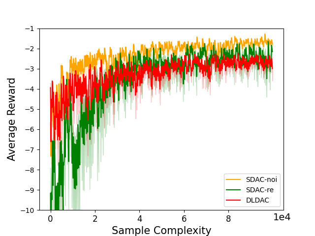
Figure 1: Averaged reward versus sample complexity and communication complexity. The vertical axis is the averaged reward over all the agents. The result is averaged over 10 Monte Carlo runs.

5 Numerical results

5.1 Experiment setting

We adopt the grounded communication environment proposed in (Mordatch & Abbeel 2018). Our task consists of NN agents and the corresponding NN landmarks inhabited in a two-dimension world, where each agent can observe the relative position of other agents and landmarks. For every discrete time step, agents take actions to move along certain directions, and receive their rewards. Agents are rewarded based on the distance to their own landmark, and penalized if they collide with other agents. The objective is to maximize the long-term averaged reward over all agents. Since we focus on decentralized setting, each agent shall not know the target landmark of others, i.e., the reward function of others. To exchange information, each agent is allowed to send their local information via a fixed communication link. Through all the experiments, the agent number NN is set to be 5, and the discount factor γ\gamma is set to be 0.950.95.

5.2 Comparison with existing decentralized AC algorithms

In this section, we compare the proposed algorithm with existing decentralized AC algorithms under the cooperative MARL setting (Chen et al. 2022; Zeng et al. 2022) in terms of sample complexity and communication complexity. In the sequel, we refer Algorithm 1 as "SDAC-re" and Algorithm 2 as "SDAC-noi" (see Appendix 2). The algorithm proposed in (Chen et al. 2022) is referred as "DLDAC", which is based on double-loop implementation. The algorithm proposed in (Zeng et al. 2022) is denoted by "TDAC-re", which is based on two-timescale step size implementation. For comparison, we also implement a noisy reward version of "TDAC-re" and denote it by "TDAC-noi".

Comparison to double-loop decentralized AC. For "SDAC-re" and "SDAC-noi", we set αk=0.01​(k+1)−0.5\alpha_{k}=0.01(k+1)^{-0.5}, βk=0.1​(k+1)−0.5,ηk=0.1​(k+1)−0.5,Kc=5,σ=0.5,Kr=2\beta_{k}=0.1(k+1)^{-0.5},\eta_{k}=0.1(k+1)^{-0.5},K_{c}=5,\sigma=0.5,K_{r}=2. For "DLDAC", we fix Tc=50T_{c}=50, Tc′=10T_{c}^{\prime}=10, T′=5T^{\prime}=5, Nc=10N_{c}=10, N=100N=100, σ=0.1\sigma=0.1 33 3 Note that we adopt the notations in (Chen et al. 2022). Here, TcT_{c} is the inner loop size, Tc′T_{c}^{\prime} is the communication number for each outer loop, T′T^{\prime} is the communication number for reward consensus, NN is the batch size for actor’s update, and NcN_{c} is the batch size for critic’s update., which is adopted by their paper (see comparisons under different hyper-parameters in Appendix A). We set α=0.01,β=0.1\alpha=0.01,\beta=0.1 for "DLDAC" since we observe that larger step sizes will result in divergence. We have to mention that such a inner loop size Tc=50T_{c}=50 in "DLDAC" is not necessarily consistent with the theory of a double-loop algorithm, in which the loop size should be proportional to 𝒪⁡(ε−1)\mathcal{O}(\varepsilon^{-1}). The sample complexity and communication complexity results are shown in Figure 1. For the sample complexity, "SDAC-noi" enjoys a faster convergence compared with "DLDAC". In terms of communication complexity, "DLDAC" achieves better performance as it applies mini-batch technique and thereby requires less communication rounds when using the same amount of samples. Such a mini-batch approach can also be adopted to our proposed algorithms. Thus, we implement a mini-batch version of our proposed algorithms, which we refer as "SDAC-noi-batch" and "SDAC-re-batch", respectively. We set 10 as the batch size for actor, critic, and reward estimator. We can see that by applying mini-batch update, these two variants achieve significantly better communication complexity compared with "DLDAC". This is because our algorithm updates actor for more times compared with "DLDAC" under the same communication rounds.

Refer to caption
Figure 2: Comparison between the proposed algorithms and two-timescale decentralized AC algorithms (Zeng et al. 2022). The results are averaged over 10 Monte Carlo runs.

Comparison with two-timescale decentralized AC. We fix Kc=1K_{c}=1, Kr=5K_{r}=5 for this experiment. We set αk=0.01​(k+1)−0.5\alpha_{k}=0.01(k+1)^{-0.5}, βk=0.1​(k+1)−0.5\beta_{k}=0.1(k+1)^{-0.5}, and ηk=0.1​(k+1)−0.5\eta_{k}=0.1(k+1)^{-0.5} for "SDAC-re" and "SDAC-noi"; we set αk=0.01​(k+1)−0.6\alpha_{k}=0.01(k+1)^{-0.6}, βk=0.1​(k+1)−0.4\beta_{k}=0.1(k+1)^{-0.4}, and ηk=0.1​(k+1)−0.4\eta_{k}=0.1(k+1)^{-0.4} for "TDAC-re" and "TDAC-noi". The sample complexity is presented in Figure 2. We can observe that the convergence speed of "SDAC-noi" is slightly better than that the two-timescale counterpart "TDAC-noi". In addition, when using reward estimator for the global reward estimation, we see that "SDAC-re" has much more stable convergence behavior than "TDAC-re", and achieves significantly higher rewards.

Refer to caption
Refer to caption
Figure 3: Ablation study on the consensus periods. The results are averaged over 10 Monte Carlo runs.

5.3 Ablation study on different choices of KcK_{c}

We compare the performance of "SDAC-noi" under different choices of consensus periods KcK_{c}. In particular, we set αk=0.01​(k+1)−0.5\alpha_{k}=0.01(k+1)^{-0.5}, βk=0.1​(k+1)−0.5\beta_{k}=0.1(k+1)^{-0.5}, Kr=2K_{r}=2, σ=0.5\sigma=0.5 and examine the consensus periods KcK_{c} of 1, 5, 10, and 20, respectively. The corresponding sample complexity and communication complexity results are summarized in Figure 3. Evidently, in terms of sample complexity, the convergence becomes slower and relatively unstable as the consensus period KcK_{c} increases. Therefore, when the communication cost is low, choosing a small KcK_{c} will yield a better performance. We also plot the communication complexity under the consensus periods of 11 and 55. We can see that the communication complexity of "cons-5" outperforms "cons-1" after 12×10312\times 10^{3} communications. Thus, when the communication cost is expensive and high averaged reward is required, one may use large KcK_{c} and run the algorithm for a relatively large number of iterations.

6 Conclusion and future direction

In this paper, we studied the convergence of fully decentralized AC algorithm under practical single-timescale update. We showed that the algorithm will maintain the optimal sample complexity of 𝒪~​(ε−2)\tilde{\mathcal{O}}(\varepsilon^{-2}) and is communication efficient. We also proposed a variant to preserve the privacy of local actions by communicating noisy rewards. Extensive simulation results demonstrate the superiority of our algorithms’ empirical performance over existing decentralized AC algorithms. However, directly extending our single-timescale AC’s analysis technique to single-timescale NAC will result in a sub-optimal sample complexity. We leave the study on improving the convergence rate and design a more efficient single-timescale NAC algorithm as promising future directions.

Acknowledgement

The authors would like to thank the Action Editor and anonymous reviewers for their detailed and constructive comments, which have helped greatly to improve the quality and presentation of the manuscript.

X. Li was partially supported by the National Natural Science Foundation of China (NSFC) under Grant No. 12201534 and 72150002, by the Shenzhen Science and Technology Program under Grant No. RCBS20210609103708017, and by the Shenzhen Institute of Artificial Intelligence and Robotics for Society (AIRS) under Grant No. AC01202101108.

References

  • Agarwal et al. (2019) Alekh Agarwal, Sham M Kakade, Jason D Lee, and Gaurav Mahajan. On the theory of policy gradient methods: Optimality, approximation, and distribution shift. ArXiv:1908.00261, 2019.
  • Agarwal et al. (2020) Alekh Agarwal, Sham M Kakade, Jason D Lee, and Gaurav Mahajan. Optimality and approximation with policy gradient methods in markov decision processes. In Conference on Learning Theory (COLT), pp. 64–66, 2020.
  • Baxter & Bartlett (2001) Jonathan Baxter and Peter L. Bartlett. Infinite-horizon policy-gradient estimation. Journal of Artificial Intelligence Research, 15:319–350, 2001.
  • Bhandari et al. (2018) Jalaj Bhandari, Daniel Russo, and Raghav Singal. A finite time analysis of temporal difference learning with linear function approximation. In Conference on Learning Theory (COLT), pp. 1691–1692, 2018.
  • Chen et al. (2021a) Tianyi Chen, Yuejiao Sun, and Wotao Yin. Closing the gap: Tighter analysis of alternating stochastic gradient methods for bilevel problems. In A. Beygelzimer, Y. Dauphin, P. Liang, and J. Wortman Vaughan (eds.), Advances in Neural Information Processing Systems, 2021a. URL https://openreview.net/forum?id=OItvP2-i9j.
  • Chen et al. (2021b) Ziyi Chen, Yi Zhou, and Rongrong Chen. Multi-agent off-policy td learning: Finite-time analysis with near-optimal sample complexity and communication complexity. arXiv preprint arXiv:2103.13147, 2021b.
  • Chen et al. (2022) Ziyi Chen, Yi Zhou, Rong-Rong Chen, and Shaofeng Zou. Sample and communication-efficient decentralized actor-critic algorithms with finite-time analysis. In International Conference on Machine Learning, pp. 3794–3834. PMLR, 2022.
  • Doya (2000) Kenji Doya. Reinforcement learning in continuous time and space. Neural Computation, 12(1):219–245, 2000.
  • Espeholt et al. (2018) Lasse Espeholt, Hubert Soyer, Remi Munos, Karen Simonyan, Vlad Mnih, Tom Ward, Yotam Doron, Vlad Firoiu, Tim Harley, Iain Dunning, et al. Impala: Scalable distributed deep-rl with importance weighted actor-learner architectures. In International Conference on Machine Learning, pp. 1407–1416. PMLR, 2018.
  • Fu et al. (2021) Zuyue Fu, Zhuoran Yang, and Zhaoran Wang. Single-timescale actor-critic provably finds globally optimal policy. In International Conference on Learning Representations, 2021. URL https://openreview.net/forum?id=pqZV_srUVmK.
  • Guo et al. (2021) Hongyi Guo, Zuyue Fu, Zhuoran Yang, and Zhaoran Wang. Decentralized single-timescale actor-critic on zero-sum two-player stochastic games. In International Conference on Machine Learning, pp. 3899–3909. PMLR, 2021.
  • Hairi et al. (2022) FNU Hairi, Jia Liu, and Songtao Lu. Finite-time convergence and sample complexity of multi-agent actor-critic reinforcement learning with average reward. In International Conference on Learning Representations, 2022.
  • Kakade (2002) Sham M Kakade. A natural policy gradient. In Proc. Advances in Neural Information Processing Systems (NIPS), pp. 1531–1538, 2002.
  • Konda & Borkar (1999) Vijaymohan R Konda and Vivek S Borkar. Actor-critic–type learning algorithms for Markov decision processes. SIAM Journal on Control and Optimization, 38(1):94–123, 1999.
  • Lillicrap et al. (2015) Timothy P Lillicrap, Jonathan J Hunt, Alexander Pritzel, Nicolas Heess, Tom Erez, Yuval Tassa, David Silver, and Daan Wierstra. Continuous control with deep reinforcement learning. arXiv preprint arXiv:1509.02971, 2015.
  • Lin et al. (2019) Yixuan Lin, Kaiqing Zhang, Zhuoran Yang, Zhaoran Wang, Tamer Başar, Romeil Sandhu, and Ji Liu. A communication-efficient multi-agent actor-critic algorithm for distributed reinforcement learning. In 2019 IEEE 58th Conference on Decision and Control (CDC), pp. 5562–5567, 2019.
  • Littman (1994) Michael L Littman. Markov games as a framework for multi-agent reinforcement learning. In Machine learning proceedings 1994, pp. 157–163. Elsevier, 1994.
  • Liu et al. (2020) Yanli Liu, Kaiqing Zhang, Tamer Basar, and Wotao Yin. An improved analysis of (variance-reduced) policy gradient and natural policy gradient methods. Advances in Neural Information Processing Systems, 33:7624–7636, 2020.
  • Lowe et al. (2017) Ryan Lowe, Yi I Wu, Aviv Tamar, Jean Harb, OpenAI Pieter Abbeel, and Igor Mordatch. Multi-agent actor-critic for mixed cooperative-competitive environments. Advances in neural information processing systems, 30, 2017.
  • Mordatch & Abbeel (2018) Igor Mordatch and Pieter Abbeel. Emergence of grounded compositional language in multi-agent populations. In Proceedings of the AAAI Conference on Artificial Intelligence, volume 32, 2018.
  • Olshevsky & Gharesifard (2023) Alex Olshevsky and Bahman Gharesifard. A small gain analysis of single timescale actor critic. To appear in SIAM Journal on Control and Optimization, 2023, 2023.
  • Omidshafiei et al. (2017) Shayegan Omidshafiei, Jason Pazis, Christopher Amato, Jonathan P How, and John Vian. Deep decentralized multi-task multi-agent reinforcement learning under partial observability. In International Conference on Machine Learning, pp. 2681–2690. PMLR, 2017.
  • Peters & Schaal (2008) Jan Peters and Stefan Schaal. Natural actor-critic. Neurocomputing, 71(7-9):1180–1190, 2008.
  • Qiu et al. (2019) Shuang Qiu, Zhuoran Yang, Jieping Ye, and Zhaoran Wang. On the finite-time convergence of actor-critic algorithm. In Optimization Foundations for Reinforcement Learning Workshop at Advances in Neural Information Processing Systems (NeurIPS), 2019.
  • Rashid et al. (2018) Tabish Rashid, Mikayel Samvelyan, Christian Schroeder, Gregory Farquhar, Jakob Foerster, and Shimon Whiteson. Qmix: Monotonic value function factorisation for deep multi-agent reinforcement learning. In International Conference on Machine Learning, pp. 4295–4304. PMLR, 2018.
  • Schulman et al. (2017) John Schulman, Filip Wolski, Prafulla Dhariwal, Alec Radford, and Oleg Klimov. Proximal policy optimization algorithms. arXiv preprint arXiv:1707.06347, 2017.
  • Shen et al. (2020) Han Shen, Kaiqing Zhang, Mingyi Hong, and Tianyi Chen. Asynchronous advantage actor critic: Non-asymptotic analysis and linear speedup. ArXiv:2012.15511, 2020.
  • Silver et al. (2017) David Silver, Julian Schrittwieser, Karen Simonyan, Ioannis Antonoglou, Aja Huang, Arthur Guez, Thomas Hubert, Lucas Baker, Matthew Lai, Adrian Bolton, et al. Mastering the game of go without human knowledge. nature, 550(7676):354–359, 2017.
  • Son et al. (2019) Kyunghwan Son, Daewoo Kim, Wan Ju Kang, David Earl Hostallero, and Yung Yi. Qtran: Learning to factorize with transformation for cooperative multi-agent reinforcement learning. In International Conference on Machine Learning, pp. 5887–5896. PMLR, 2019.
  • Sun et al. (2020) Jun Sun, Gang Wang, Georgios B Giannakis, Qinmin Yang, and Zaiyue Yang. Finite-sample analysis of decentralized temporal-difference learning with linear function approximation. In Proc. International Conference on Artificial Intelligence and Statistics (AISTATS), pp. 4485–4495, 2020.
  • Sutton et al. (2000) Richard S Sutton, David A McAllester, Satinder P Singh, and Yishay Mansour. Policy gradient methods for reinforcement learning with function approximation. In Proc. Advances in Neural Information Processing Systems (NIPS), pp. 1057–1063, 2000.
  • Tsitsiklis & Van Roy (1997) John N Tsitsiklis and Benjamin Van Roy. Analysis of temporal-diffference learning with function approximation. In Advances in neural information processing systems (NIPS), pp. 1075–1081, 1997.
  • Vinyals et al. (2019) Oriol Vinyals, Igor Babuschkin, Wojciech M Czarnecki, Michaël Mathieu, Andrew Dudzik, Junyoung Chung, David H Choi, Richard Powell, Timo Ewalds, Petko Georgiev, et al. Grandmaster level in starcraft ii using multi-agent reinforcement learning. Nature, 575(7782):350–354, 2019.
  • Wang et al. (2021) Yue Wang, Shaofeng Zou, and Yi Zhou. Non-asymptotic analysis for two time-scale TDC with general smooth function approximation. In M. Ranzato, A. Beygelzimer, Y. Dauphin, P.S. Liang, and J. Wortman Vaughan (eds.), Advances in Neural Information Processing Systems, volume 34, pp. 9747–9758. Curran Associates, Inc., 2021. URL https://proceedings.neurips.cc/paper/2021/file/50e207ab6946b5d78b377ae0144b9e07-Paper.pdf.
  • Wu et al. (2020) Yue Frank Wu, Weitong Zhang, Pan Xu, and Quanquan Gu. A finite-time analysis of two time-scale actor-critic methods. Advances in Neural Information Processing Systems, 33:17617–17628, 2020.
  • Xu et al. (2019) Pan Xu, Felicia Gao, and Quanquan Gu. An improved convergence analysis of stochastic variance-reduced policy gradient. In Proc. International Conference on Uncertainty in Artificial Intelligence (UAI), 2019.
  • Xu & Liang (2021) Tengyu Xu and Yingbin Liang. Sample complexity bounds for two timescale value-based reinforcement learning algorithms. In International Conference on Artificial Intelligence and Statistics, pp. 811–819. PMLR, 2021.
  • Xu et al. (2020) Tengyu Xu, Zhe Wang, and Yingbin Liang. Improving sample complexity bounds for (natural) actor-critic algorithms. In Proc. Advances in Neural Information Processing Systems (NeurIPS), volume 33, 2020.
  • Xu et al. (2021) Tengyu Xu, Zhuoran Yang, Zhaoran Wang, and Yingbin Liang. Doubly robust off-policy actor-critic: Convergence and optimality. ArXiv:2102.11866, 2021.
  • Yu et al. (2019) Chao Yu, Xin Wang, Xin Xu, Minjie Zhang, Hongwei Ge, Jiankang Ren, Liang Sun, Bingcai Chen, and Guozhen Tan. Distributed multiagent coordinated learning for autonomous driving in highways based on dynamic coordination graphs. IEEE Transactions on Intelligent Transportation Systems, 21(2):735–748, 2019.
  • Zeng et al. (2022) Siliang Zeng, Tianyi Chen, Alfredo Garcia, and Mingyi Hong. Learning to coordinate in multi-agent systems: A coordinated actor-critic algorithm and finite-time guarantees. In Learning for Dynamics and Control Conference, pp. 278–290. PMLR, 2022.
  • Zhang et al. (2020) Haifeng Zhang, Weizhe Chen, Zeren Huang, Minne Li, Yaodong Yang, Weinan Zhang, and Jun Wang. Bi-level actor-critic for multi-agent coordination. In Proceedings of the AAAI Conference on Artificial Intelligence, volume 34, pp. 7325–7332, 2020.
  • Zhang et al. (2018) Kaiqing Zhang, Zhuoran Yang, Han Liu, Tong Zhang, and Tamer Basar. Fully decentralized multi-agent reinforcement learning with networked agents. In International Conference on Machine Learning, pp. 5872–5881. PMLR, 2018.
  • Zhang et al. (2019) Kaiqing Zhang, Alec Koppel, Hao Zhu, and Tamer Başar. Global convergence of policy gradient methods to (almost) locally optimal policies. arXiv preprint arXiv:1906.08383, 2019.
  • Zhang et al. (2021) Kaiqing Zhang, Zhuoran Yang, and Tamer Başar. Multi-agent reinforcement learning: A selective overview of theories and algorithms. Handbook of Reinforcement Learning and Control, pp. 321–384, 2021.
Refer to caption
(a) Different actor’s batch sizes.
Refer to caption
(b) Different critic’s batch sizes.
Refer to caption
(c) Different loop sizes.
Figure 4: Comparison between the proposed algorithms and the double-loop decentralized AC algorithm that uses mini-batch update. The results are averaged over 10 Monte Carlo runs.

Appendix A Additional simulation results

In this section, we provide more experiments which compare the proposed algorithms with double-loop based decentralized AC algorithm under different batch sizes and inner loop sizes.

  1. 1.

    Actor’s batch size. We fix Tc=50T_{c}=50, Tc′=10T_{c}^{\prime}=10, Nc=10N_{c}=10, 44 4 Note that we adopt the notations in (Chen et al. 2022). Here, TcT_{c} is the inner loop size, Tc′T_{c}^{\prime} is the communication number for each outer loop, NN is the batch size for actor’s update, and NcN_{c} is the batch size for critic’s update. which is adopted by (Chen et al. 2022). We examine values of NN in {10,50,100}\{10,50,100\}. The results are in Figure 4(a). We observe that the best choice of actor’s batch size NN is 5050, and the proposed "SDAC-noi" converges faster than it in terms of sample complexity.

  2. 2.

    Critic’s batch size. We fix Tc=50T_{c}=50, Tc′=10T_{c}^{\prime}=10, N=100N=100, which is adopted by (Chen et al. 2022). We examine values of NcN_{c} in {2,10,50}\{2,10,50\}. The results are shown in Figure 4(b). As we can see, "DLDAC" with smaller critic’s batch sizes can achieve better sample complexity, indicating that the variance of critic’s update is relatively small and the mini-batch update is not needed for this task. Our proposed "SDAC-noi" achieves better convergence compared with the double-loop decentralized AC under different choices of NcN_{c}.

  3. 3.

    Inner loop size. We fix Tc′=10T_{c}^{\prime}=10, N=100N=100, Nc=10N_{c}=10, which is adopted by (Chen et al. 2022). We examine values of TcT_{c} in {5,20}\{5,20\}. The results are shown in Figure 4(c). We can see that the proposed "SDAC-noi" enjoys a better convergence in terms of sample complexity.

Appendix B Auxiliary lemmas

In this section, we provide some auxiliary lemmas, which serves as the preliminary for the proof of main theorems and lemmas.

The following two lemmas present the Lipschitz properties of the objective function and value function.

Lemma 4 ((Zhang et al. 2019), Lemma 3.2).

Suppose Assumption 3 holds, then there exists a positive constant LL such that for any policy parameter θ1\theta_{1} and θ2\theta_{2}, we have ‖∇J​(θ1)−∇J​(θ2)‖≤L​‖θ1−θ2‖\|\nabla J(\theta_{1})-\nabla J(\theta_{2})\|\leq L\|\theta_{1}-\theta_{2}\|.

Lemma 5 ((Shen et al. 2020), Lemma 4).

Suppose Assumption 3 holds, for any policy parameter θ1,θ2\theta_{1},\theta_{2} and s∈𝒮s\in\mathcal{S}, there exits a positive constant LVL_{V} such that

‖∇Vπθ1​(s)‖\displaystyle\|\nabla V_{\pi_{\theta_{1}}}(s)\| ≤LV\displaystyle\leq L_{V}
|Vπθ1​(s)−Vπθ2​(s)|\displaystyle|V_{\pi_{\theta_{1}}}(s)-V_{\pi_{\theta_{2}}}(s)| ≤LV​‖θ1−θ2‖.\displaystyle\leq L_{V}\|\theta_{1}-\theta_{2}\|.

The next lemma shows that the stationary distribution is Lipschitz continuous with respect to policy.

Lemma 6 ((Wu et al. 2020), Lemma B.1).

For any policy parameter θ1\theta_{1} and θ2\theta_{2}, it holds that

dT​V​(μθ1,μθ2)\displaystyle d_{TV}(\mu_{\theta_{1}},\mu_{\theta_{2}}) ≤|𝒜|​Lπ​(logρ⁡κ−1+(1−ρ)−1)​‖θ1−θ2‖\displaystyle\leq|\mathcal{A}|L_{\pi}(\log_{\rho}\kappa^{-1}+(1-\rho)^{-1})\|\theta_{1}-\theta_{2}\|
dT​V​(μθ1⊗πθ1,μθ2⊗πθ2)\displaystyle d_{TV}(\mu_{\theta_{1}}\otimes\pi_{\theta_{1}},\mu_{\theta_{2}}\otimes\pi_{\theta_{2}}) ≤|𝒜|​Lπ​(1+logρ⁡κ−1+(1−ρ)−1)​‖θ1−θ2‖\displaystyle\leq|\mathcal{A}|L_{\pi}(1+\log_{\rho}\kappa^{-1}+(1-\rho)^{-1})\|\theta_{1}-\theta_{2}\|
dT​V​(μθ1⊗πθ1⊗𝒫,μθ2⊗πθ2⊗𝒫)\displaystyle d_{TV}(\mu_{\theta_{1}}\otimes\pi_{\theta_{1}}\otimes\mathcal{P},\mu_{\theta_{2}}\otimes\pi_{\theta_{2}}\otimes\mathcal{P}) ≤|𝒜|​Lπ​(1+logρ⁡κ−1+(1−ρ)−1)​‖θ1−θ2‖.\displaystyle\leq|\mathcal{A}|L_{\pi}(1+\log_{\rho}\kappa^{-1}+(1-\rho)^{-1})\|\theta_{1}-\theta_{2}\|.

We will define Lμ:=|𝒜|​Lπ​(logρ⁡κ−1+(1−ρ)−1)L_{\mu}:=|\mathcal{A}|L_{\pi}(\log_{\rho}\kappa^{-1}+(1-\rho)^{-1}) for the proof of main theorems and lemmas.

The following lemma characterizes the geometric mixing of the Markov chain.

Lemma 7 ((Shen et al. 2020), Lemma 1).

Suppose Assumption 4 holds, then there exists κ>0,ρ∈[0,1]\kappa>0,\rho\in[0,1] such that for any policy parameter θ\theta we have

sups0∈𝒮dT​V(ℙ((sk,ak,sk+1)∈⋅|s0,πθ),μθ⊗πθ⊗𝒫)≤κρk,\displaystyle\sup_{s_{0}\in\mathcal{S}}d_{TV}(\mathbb{P}((s_{k},a_{k},s_{k+1})\in\cdot|s_{0},\pi_{\theta}),\mu_{\theta}\otimes\pi_{\theta}\otimes\mathcal{P})\leq\kappa\rho^{k},

where μθ\mu_{\theta} is the stationary distribution induced by πθ\pi_{\theta} and transition kernel 𝒫(⋅|s,a)\mathcal{P}(\cdot|s,a).

The next lemma bounds the error of the discounted state-visitation distribution and the stationary distribution.

Lemma 8 ((Shen et al. 2020), Lemma 2).

Suppose Assumption 4 holds, then for any policy parameter θ\theta, there exists κ>0,ρ∈[0,1]\kappa>0,\rho\in[0,1] such that

dT​V​(dπθ,μπθ)≤2​(logρ⁡κ−1+11−ρ)​(1−γ).d_{TV}(d_{\pi_{\theta}},\mu_{\pi_{\theta}})\leq 2(\log_{\rho}{\kappa^{-1}}+\frac{1}{1-\rho})(1-\gamma).

The following lemma bounds the total variation distance between state distribution under a fixed policy and that under an updating policy. The lemma is used for analyzing the sampling error.

Lemma 9.

Consider the Markov chain:

sk−z→θk−zak−z→𝒫sk−z+1→θk−z+1ak−z+1⋯→θk−1ak−1→𝒫sk→θkak→𝒫sk+1.s_{k-z}\xrightarrow{\theta_{k-z}}a_{k-z}\xrightarrow{\mathcal{P}}s_{k-z+1}\xrightarrow{\theta_{k-z+1}}a_{k-z+1}\cdots\xrightarrow{\theta_{k-1}}a_{k-1}\xrightarrow{\mathcal{P}}s_{k}\xrightarrow{\theta_{k}}a_{k}\xrightarrow{\mathcal{P}}s_{k+1}.

Also consider the auxiliary Markov chain with fixed policy:

sk−z→θk−zak−z→𝒫sk−z+1→θk−za~k−z+1⋯→θk−za~k−1→𝒫s~k→θk−za~k→𝒫s~k+1.s_{k-z}\xrightarrow{\theta_{k-z}}a_{k-z}\xrightarrow{\mathcal{P}}s_{k-z+1}\xrightarrow{\theta_{k-z}}\tilde{a}_{k-z+1}\cdots\xrightarrow{\theta_{k-z}}\tilde{a}_{k-1}\xrightarrow{\mathcal{P}}\tilde{s}_{k}\xrightarrow{\theta_{k-z}}\tilde{a}_{k}\xrightarrow{\mathcal{P}}\tilde{s}_{k+1}.

Let ξk:=(sk,ak,sk+1)\xi_{k}:=(s_{k},a_{k},s_{k+1}) be sampled from chain 1, and ξ~k:=(s~k,a~k,s~k+1)\tilde{\xi}_{k}:=(\tilde{s}_{k},\tilde{a}_{k},\tilde{s}_{k+1}) be sampled from chain 2. Then we have

dT​V(ℙ(ξk∈⋅|θk−z,sk−z+1),ℙ(ξ~k∈⋅|θk−z,sk−z+1))≤12∑m=0z−1|𝒜|Lπ∥θk−m−θk−z∥.\displaystyle d_{TV}(\mathbb{P}(\xi_{k}\in\cdot|\theta_{k-z},s_{k-z+1}),\mathbb{P}(\tilde{\xi}_{k}\in\cdot|\theta_{k-z},s_{k-z+1}))\leq\frac{1}{2}\sum_{m=0}^{z-1}|\mathcal{A}|L_{\pi}\|\theta_{k-m}-\theta_{k-z}\|.
Proof.
dT​V(ℙ(ξk∈⋅),ℙ(ξ~k∈⋅))\displaystyle\quad d_{TV}(\mathbb{P}(\xi_{k}\in\cdot),\mathbb{P}(\tilde{\xi}_{k}\in\cdot))
=12​∫s∈𝒮∫s′∈𝒮∑a∈𝒜|ℙ⁡(sk=𝑑s,ak=a,sk+1=d​s′)−ℙ⁡(s~k=𝑑s,a~k=a,s~k+1=d​s′)|\displaystyle=\frac{1}{2}\int_{s\in\mathcal{S}}\int_{s^{\prime}\in\mathcal{S}}\sum_{a\in\mathcal{A}}|\mathbb{P}(s_{k}=ds,a_{k}=a,s_{k+1}=ds^{\prime})-\mathbb{P}(\tilde{s}_{k}=ds,\tilde{a}_{k}=a,\tilde{s}_{k+1}=ds^{\prime})|
=12​∫s∈𝒮∑a∈𝒜|ℙ⁡(sk=𝑑s,ak=a)−ℙ⁡(s~k=𝑑s,a~k=a)|​∫s′∈𝒮ℙ⁡(sk+1=d​s′|sk=𝑑s,ak=a)\displaystyle=\frac{1}{2}\int_{s\in\mathcal{S}}\sum_{a\in\mathcal{A}}|\mathbb{P}(s_{k}=ds,a_{k}=a)-\mathbb{P}(\tilde{s}_{k}=ds,\tilde{a}_{k}=a)|\int_{s^{\prime}\in\mathcal{S}}\mathbb{P}(s_{k+1}=ds^{\prime}|s_{k}=ds,a_{k}=a)
=12​∫s∈𝒮∑a∈𝒜|ℙ⁡(sk=𝑑s,ak=a)−ℙ⁡(s~k=𝑑s,a~k=a)|\displaystyle=\frac{1}{2}\int_{s\in\mathcal{S}}\sum_{a\in\mathcal{A}}|\mathbb{P}(s_{k}=ds,a_{k}=a)-\mathbb{P}(\tilde{s}_{k}=ds,\tilde{a}_{k}=a)|
=12​∫s∈𝒮∑a∈𝒜|ℙ⁡(sk=𝑑s)​πθk​(a|𝑑s)−ℙ⁡(s~k=𝑑s)​πθk−z​(a|𝑑s)|\displaystyle=\frac{1}{2}\int_{s\in\mathcal{S}}\sum_{a\in\mathcal{A}}|\mathbb{P}(s_{k}=ds)\pi_{\theta_{k}}(a|ds)-\mathbb{P}(\tilde{s}_{k}=ds)\pi_{\theta_{k-z}}(a|ds)|
≤12​∫s∈𝒮∑a∈𝒜|ℙ⁡(sk=𝑑s)​πθk​(a|𝑑s)−ℙ⁡(sk=𝑑s)​πθk−z​(a|𝑑s)|\displaystyle\leq\frac{1}{2}\int_{s\in\mathcal{S}}\sum_{a\in\mathcal{A}}|\mathbb{P}(s_{k}=ds)\pi_{\theta_{k}}(a|ds)-\mathbb{P}(s_{k}=ds)\pi_{\theta_{k-z}}(a|ds)|
+12∫s∈𝒮∑a∈𝒜|ℙ(sk=ds)πθk−z(a|ds)−ℙ(s~k=ds)πθk−z(a|ds)|\displaystyle\quad+\frac{1}{2}\int_{s\in\mathcal{S}}\sum_{a\in\mathcal{A}}|\mathbb{P}(s_{k}=ds)\pi_{\theta_{k-z}}(a|ds)-\mathbb{P}(\tilde{s}_{k}=ds)\pi_{\theta_{k-z}}(a|ds)|
≤12​∫s∈𝒮|𝒜|​Lπ​‖θk−θk−z‖​ℙ​(sk=𝑑s)\displaystyle\leq\frac{1}{2}\int_{s\in\mathcal{S}}|\mathcal{A}|L_{\pi}\|\theta_{k}-\theta_{k-z}\|\mathbb{P}(s_{k}=ds)
+12∫s∈𝒮|ℙ(sk=ds)−ℙ(s~k=ds)|∑a∈𝒜πθk−z(a|ds)\displaystyle\quad+\frac{1}{2}\int_{s\in\mathcal{S}}|\mathbb{P}(s_{k}=ds)-\mathbb{P}(\tilde{s}_{k}=ds)|\sum_{a\in\mathcal{A}}\pi_{\theta_{k-z}}(a|ds)
=12|𝒜|Lπ∥θk−θk−z∥+dT​V(ℙ(sk∈⋅),ℙ(s~k∈⋅)).\displaystyle=\frac{1}{2}|\mathcal{A}|L_{\pi}\|\theta_{k}-\theta_{k-z}\|+d_{TV}(\mathbb{P}(s_{k}\in\cdot),\mathbb{P}(\tilde{s}_{k}\in\cdot)). (20)

The second term can be bounded as

dT​V(ℙ(sk∈⋅),ℙ(s~k∈⋅))\displaystyle d_{TV}(\mathbb{P}(s_{k}\in\cdot),\mathbb{P}(\tilde{s}_{k}\in\cdot))
=12​∫s′∈𝒮|ℙ⁡(sk=𝑑s)−ℙ⁡(s~k=𝑑s)|\displaystyle=\frac{1}{2}\int_{s^{\prime}\in\mathcal{S}}|\mathbb{P}(s_{k}=ds)-\mathbb{P}(\tilde{s}_{k}=ds)|
=12​∫s′∈𝒮|∑a∈𝒜∫s∈𝒮ℙ⁡(sk−1=𝑑s,ak−1=a,sk=d​s′)−ℙ⁡(s~k−1=𝑑s,a~k−1=a,s~k=d​s′)|\displaystyle=\frac{1}{2}\int_{s^{\prime}\in\mathcal{S}}|\sum_{a\in\mathcal{A}}\int_{s\in\mathcal{S}}\mathbb{P}(s_{k-1}=ds,a_{k-1}=a,s_{k}=ds^{\prime})-\mathbb{P}(\tilde{s}_{k-1}=ds,\tilde{a}_{k-1}=a,\tilde{s}_{k}=ds^{\prime})|
≤12​∫s′∈𝒮∑a∈𝒜∫s∈𝒮|ℙ⁡(sk−1=𝑑s,ak−1=a,sk=d​s′)−ℙ⁡(s~k−1=𝑑s,a~k−1=a,s~k=d​s′)|\displaystyle\leq\frac{1}{2}\int_{s^{\prime}\in\mathcal{S}}\sum_{a\in\mathcal{A}}\int_{s\in\mathcal{S}}|\mathbb{P}(s_{k-1}=ds,a_{k-1}=a,s_{k}=ds^{\prime})-\mathbb{P}(\tilde{s}_{k-1}=ds,\tilde{a}_{k-1}=a,\tilde{s}_{k}=ds^{\prime})|
=dT​V(ℙ(ξk−1∈⋅),ℙ(ξ~k−1∈⋅)).\displaystyle=d_{TV}(\mathbb{P}(\xi_{k-1}\in\cdot),\mathbb{P}(\tilde{\xi}_{k-1}\in\cdot)). (21)

Combined (20) and (21), we obtain

dT​V(ℙ(ξk∈⋅),ℙ(ξ~k∈⋅))≤dT​V(ℙ(ξk−1∈⋅),ℙ(ξ~k−1∈⋅))+12|𝒜|Lπ|θk−θk−z∥.\displaystyle d_{TV}(\mathbb{P}(\xi_{k}\in\cdot),\mathbb{P}(\tilde{\xi}_{k}\in\cdot))\leq d_{TV}(\mathbb{P}(\xi_{k-1}\in\cdot),\mathbb{P}(\tilde{\xi}_{k-1}\in\cdot))+\frac{1}{2}|\mathcal{A}|L_{\pi}|\theta_{k}-\theta_{k-z}\|.

Sum over z−1z-1 steps, we obtain

dT​V(ℙ(ξk∈⋅),ℙ(ξ~k∈⋅))\displaystyle d_{TV}(\mathbb{P}(\xi_{k}\in\cdot),\mathbb{P}(\tilde{\xi}_{k}\in\cdot)) ≤dT​V(ℙ(ξk−z∈⋅),ℙ(ξ~k−z∈⋅))+12∑m=0z−1|𝒜|Lπ∥θk−m−θk−z∥\displaystyle\leq d_{TV}(\mathbb{P}(\xi_{k-z}\in\cdot),\mathbb{P}(\tilde{\xi}_{k-z}\in\cdot))+\frac{1}{2}\sum_{m=0}^{z-1}|\mathcal{A}|L_{\pi}\|\theta_{k-m}-\theta_{k-z}\|
=12​∑m=0z−1|𝒜|​Lπ​‖θk−m−θk−z‖.\displaystyle=\frac{1}{2}\sum_{m=0}^{z-1}|\mathcal{A}|L_{\pi}\|\theta_{k-m}-\theta_{k-z}\|.

∎

Next, we present some mathematical facts that are useful in our analysis.

Lemma 10 ((Chen et al. 2021b), Lemma F.3).

For a doubly stochastic matrix W∈ℝN×NW\in\mathbb{R}^{N\times N} and the difference matrix Q:=I−1N​11T{Q:=I-\frac{1}{N}\textbf{1}\textbf{1}^{T}}, it holds that for any matrix H∈ℝN×NH\in\mathbb{R}^{N\times N}, ‖Wk​H‖≤νk​‖Q​H‖\|W^{k}H\|\leq\nu^{k}\|QH\|, where ν\nu is the second largest singular value of WW.

Lemma 11 (descent lemma in high dimension).

Consider the mapping F:ℝn→ℝmF:\mathbb{R}^{n}\rightarrow\mathbb{R}^{m}. If there exists a positive constant LL such that

‖∇F​(x)−∇F​(y)‖F≤L​‖x−y‖,∀x,y∈dom​(F),\displaystyle\|\nabla F(x)-\nabla F(y)\|_{F}\leq L\|x-y\|,\ \forall x,y\in\text{dom}(F), (22)

then the following holds

‖F⁡(y)−F⁡(x)−∇F​(x)​(y−x)‖≤L2​m​‖y−x‖2.\displaystyle\|F(y)-F(x)-\nabla F(x)(y-x)\|\leq\frac{L}{2}\sqrt{m}\|y-x\|^{2}.
Proof.

Observe that (22) directly implies the smoothness of each entry FiF_{i}:

‖∇Fi​(x)−∇Fi​(y)‖≤‖∇F​(x)−∇F​(y)‖F≤L​‖x−y‖.\|\nabla F_{i}(x)-\nabla F_{i}(y)\|\leq\|\nabla F(x)-\nabla F(y)\|_{F}\leq L\|x-y\|.

Define

zi(x,y):=Fi(y)−Fi(x)−∇Fi(x)T(y−x).z_{i}(x,y):=F_{i}(y)-F_{i}(x)-\nabla F_{i}(x)^{T}(y-x).

We have

‖F⁡(y)−F⁡(x)−∇F​(x)​(y−x)‖\displaystyle\|F(y)-F(x)-\nabla F(x)(y-x)\| =∑i=1mzi​(x,y)2\displaystyle=\sqrt{\sum_{i=1}^{m}z_{i}(x,y)^{2}}
≤m​(L2​‖y−x‖2)2\displaystyle\leq\sqrt{m(\frac{L}{2}\|y-x\|^{2})^{2}}
=L12​m​‖y−x‖2,\displaystyle=\frac{L_{1}}{2}\sqrt{m}\|y-x\|^{2},

where the inequality follows the descent lemma. ∎

Lemma 12 (Lipschitz property of multiplication).

Suppose f⁡(x)f(x) and g⁡(x)g(x) are two functions bounded by CfC_{f} and CgC_{g}, and are LfL_{f}- and LgL_{g}-Lipschitz continuous, then f⁡(x)​g​(x)f(x)g(x) is Cf​Lg+Cg​LfC_{f}L_{g}+C_{g}L_{f}-Lipschitz continuous.

Proof.
‖f⁡(x1)​g​(x1)−f⁡(x2)​g​(x2)‖\displaystyle\|f(x_{1})g(x_{1})-f(x_{2})g(x_{2})\| =‖f⁡(x1)​g​(x1)−f⁡(x1)​g​(x2)+f⁡(x1)​g​(x2)−f⁡(x2)​g​(x2)‖\displaystyle=\|f(x_{1})g(x_{1})-f(x_{1})g(x_{2})+f(x_{1})g(x_{2})-f(x_{2})g(x_{2})\|
≤‖f⁡(x1)​‖‖g⁡(x1)−g⁡(x2)‖+‖​f​(x1)−f⁡(x2)‖​‖g⁡(x2)‖\displaystyle\leq\|f(x_{1})\|\|g(x_{1})-g(x_{2})\|+\|f(x_{1})-f(x_{2})\|\|g(x_{2})\|
≤(Cf​Lg+Cg​Lf)​‖x1−x2‖.\displaystyle\leq(C_{f}L_{g}+C_{g}L_{f})\|x_{1}-x_{2}\|.

∎

Lemma 13 (invertible property of matrix).

If a square matrix AA satisfies limt→∞At=0\lim_{t\rightarrow\infty}A^{t}=0, or equivalently, |λ⁡(A)|<1|\lambda(A)|<1, then I−AI-A is invertible.

Proof.
(I−A)​limt→∞∑i=0tAt\displaystyle(I-A)\lim_{t\rightarrow\infty}\sum_{i=0}^{t}A^{t} =limt→∞[∑i=0tAt−∑i=1t+1At]\displaystyle=\lim_{t\rightarrow\infty}[\sum_{i=0}^{t}A^{t}-\sum_{i=1}^{t+1}A^{t}]
=I−limt→∞At+1\displaystyle=I-\lim_{t\rightarrow\infty}A^{t+1}
=I\displaystyle=I

Since II is invertible, by the rank inequality rank​(A​B)≤min⁡(rank​(A),rank​(B))\text{rank}(AB)\leq\min(\text{rank}(A),\text{rank}(B)), I−AI-A and limt→∞∑i=0tAt\lim_{t\rightarrow\infty}\sum_{i=0}^{t}A^{t} will be full rank and thereby invertible. ∎

Appendix C Supporting lemmas

Before proceeding to the analysis of critic variables, we justify the uniqueness of fix point for critic and reward estimator variables under the update (5) and (8), respectively. Define the following notations

Aθ,ϕ\displaystyle A_{\theta,\phi} :=𝔼⁡[ϕ⁡(s)​(γ​ϕ​(s′)T−ϕ​(s)T)],\displaystyle:=\mathbb{E}[\phi(s)(\gamma\phi(s^{\prime})^{T}-\phi(s)^{T})], (23)
Aθ,φ\displaystyle A_{\theta,\varphi} :=𝔼⁡[φ⁡(s,a)​φ​(s,a)T],\displaystyle:=\mathbb{E}[\varphi(s,a)\varphi(s,a)^{T}],
bθ,ϕ\displaystyle b_{\theta,\phi} :=𝔼⁡[ϕ⁡(s)​r¯​(s,a)],\displaystyle:=\mathbb{E}[\phi(s)\bar{r}(s,a)],
bθ,φ\displaystyle b_{\theta,\varphi} :=𝔼⁡[φ⁡(s,a)​r¯​(s,a)],\displaystyle:=\mathbb{E}[\varphi(s,a)\bar{r}(s,a)],

with expectation taken from s∼μθ​(s),a∼πθ,s′∼𝒫s\sim\mu_{\theta}(s),a\sim\pi_{\theta},s^{\prime}\sim\mathcal{P}. The optimal critic and reward estimator variables given policy θ\theta will satisfy Aθ,ϕ​ω∗​(θ)+bθ,ϕ=0;Aθ,φ​λ∗​(θ)+bθ,φ=0.A_{\theta,\phi}\omega^{*}(\theta)+b_{\theta,\phi}=0;A_{\theta,\varphi}\lambda^{*}(\theta)+b_{\theta,\varphi}=0. By Assumption 2, Aθ,ϕA_{\theta,\phi} and Aθ,φA_{\theta,\varphi} are negative definite with largest eigenvalue λϕ\lambda_{\phi} and λφ\lambda_{\varphi}, which ensures the unique solution ω∗​(θ)=−Aθ,ϕ−1​bθ,ϕ;λ∗​(θ)=−Aθ,φ−1​bθ,φ.\omega^{*}(\theta)=-A_{\theta,\phi}^{-1}b_{\theta,\phi};\lambda^{*}(\theta)=-A_{\theta,\varphi}^{-1}b_{\theta,\varphi}. Let Rω:=rmaxλϕ,Rλ:=rmaxλφR_{\omega}:=\frac{r_{\max}}{\lambda_{\phi}},R_{\lambda}:=\frac{r_{\max}}{\lambda_{\varphi}}. Then the norm of optimal solutions will be bounded as ‖ω∗​(θ)‖≤Rω,‖λ∗​(θ)‖≤Rλ\|\omega^{*}(\theta)\|\leq R_{\omega},\ \|\lambda^{*}(\theta)\|\leq R_{\lambda}, which justifies the projection step of the Algorithm 1. In practice, the knowledge of λϕ\lambda_{\phi} and λφ\lambda_{\varphi} may not be available. One can estimate projection radius online using the methods proposed in Section 8.2 of (Bhandari et al. 2018).

We slightly abuse the notation by overwriting VπθV_{\pi_{\theta}} as VθV_{\theta}. To study the error of critic, we introduce the following notations (crf. ξ:=(s,a,s′)\xi:=(s,a,s^{\prime}))

δi​(ξ,θ)\displaystyle\delta^{i}(\xi,\theta) :=ri​(s,a)+γ​Vθ​(s′)−Vθ​(s)\displaystyle:=r^{i}(s,a)+\gamma V_{\theta}(s^{\prime})-V_{\theta}(s)
δ⁡(ξ,θ)\displaystyle\delta(\xi,\theta) :=r¯​(s,a)+γ​Vθ​(s′)−Vθ​(s)\displaystyle:=\bar{r}(s,a)+\gamma V_{\theta}(s^{\prime})-V_{\theta}(s)
δ~​(ξ,ω)\displaystyle\tilde{\delta}(\xi,\omega) :=r¯​(s,a)+γ​ϕ​(s′)T​ω−ϕ​(s)T​ω\displaystyle:=\bar{r}(s,a)+\gamma\phi(s^{\prime})^{T}\omega-\phi(s)^{T}\omega
δ^​(ξ,ω,λ)\displaystyle\hat{\delta}(\xi,\omega,\lambda) :=φ​(s,a)T​λ+γ​ϕ​(s′)T​ω−ϕ​(s)T​ω,\displaystyle:=\varphi(s,a)^{T}\lambda+\gamma\phi(s^{\prime})^{T}\omega-\phi(s)^{T}\omega, (24)

For the ease of expression, we further define

gai​(ξ,ω,λ)\displaystyle g_{a}^{i}(\xi,\omega,\lambda) :=δ^​(ξ,ω,λ)​ψθi​(s,ai),\displaystyle:=\hat{\delta}(\xi,\omega,\lambda)\psi_{\theta^{i}}(s,a^{i}),
gci​(ξ,ω)\displaystyle g_{c}^{i}(\xi,\omega) :=δi​(ξ,ω)​ϕ​(s),\displaystyle:=\delta^{i}(\xi,\omega)\phi(s),
g¯c​(ξ,ω)\displaystyle\bar{g}_{c}(\xi,\omega) :=δ~​(ξ,ω)​ϕ​(s),\displaystyle:=\tilde{\delta}(\xi,\omega)\phi(s),
gc​(θ,ω)\displaystyle g_{c}(\theta,\omega) :=𝔼ξ∼μθ​[g¯c​(ξ,ω)].\displaystyle:=\mathbb{E}_{\xi\sim\mu_{\theta}}[\bar{g}_{c}(\xi,\omega)]. (25)

C.1 Error of critic

The following lemmas and propositions serves as the preliminary for establishing the approximate descent property of the critic variables’ optimal gap.

Proposition 1 (Lipschitz continuity of ω∗​(θ)\omega^{*}(\theta) (Wu et al. 2020)).

Suppose Assumptions 1, 2, 3, and 4 hold, then there exists a positive constant LωL_{\omega} such that for any θ1,θ2∈ℝN​dθ\theta_{1},\theta_{2}\in\mathbb{R}^{Nd_{\theta}}, we have

‖ω∗​(θ1)−ω∗​(θ2)‖≤Lω​‖θ1−θ2‖.\displaystyle\|\omega^{*}(\theta_{1})-\omega^{*}(\theta_{2})\|\leq L_{\omega}\|\theta_{1}-\theta_{2}\|.
Lemma 14 (smoothness of stationary distribution).

For any θ,θ′∈ℝd\theta,\theta^{\prime}\in\mathbb{R}^{d}, there exists a positive constant Lμ,2L_{\mu,2} such that ‖∇μθ​(s)−∇μθ′​(s)‖≤Lμ,2​‖θ−θ′‖\|\nabla\mu_{\theta}(s)-\nabla\mu_{\theta^{\prime}}(s)\|\leq L_{\mu,2}\|\theta-\theta^{\prime}\|.

The proof of this Lemma consists of two main steps: 1) Derive the expression of the gradient and 2) establish that the gradient is Lipschitz continuous. For the first part, we follow the main idea in (Baxter & Bartlett 2001).

Proof.

For a given policy πθ\pi_{\theta}, we define the transition probability Pθ​(s|s′):=∑aπθ​(a|s′)​P​(s|s′,a)P_{\theta}(s|s^{\prime}):=\sum_{a}\pi_{\theta}(a|s^{\prime})P(s|s^{\prime},a). By the Assumption 4, there exists a stationary distribution μθ​(s)\mu_{\theta}(s) which satisfies for all state ss

μθ​(s)=∑s′∈𝒮μθ​(s′)​Pθ​(s|s′)\displaystyle\mu_{\theta}(s)=\sum_{s^{\prime}\in\mathcal{S}}\mu_{\theta}(s^{\prime})P_{\theta}(s|s^{\prime}) (26)

Define the following notations

μθ\displaystyle\mu_{\theta} :=[μθ​(s1),μθ​(s2),⋯,μθ​(sn)]T\displaystyle:=[\mu_{\theta}(s_{1}),\mu_{\theta}(s_{2}),\cdots,\mu_{\theta}(s_{n})]^{T} ℝ|𝒮|×1\displaystyle\mathbb{R}^{|\mathcal{S}|\times 1}
Pθ​(s)\displaystyle P_{\theta}(s) :=[Pθ​(s|s1),Pθ​(s|s2),⋯,Pθ​(s|sn)]T\displaystyle:=[P_{\theta}(s|s_{1}),P_{\theta}(s|s_{2}),\cdots,P_{\theta}(s|s_{n})]^{T} ℝ|𝒮|×1\displaystyle\mathbb{R}^{|\mathcal{S}|\times 1}
P⁡(θ)\displaystyle P(\theta) :=[Pθ​(s1),Pθ​(s2),⋯,Pθ​(sn)]\displaystyle:=[P_{\theta}(s_{1}),P_{\theta}(s_{2}),\cdots,P_{\theta}(s_{n})] ℝ|𝒮|×|𝒮|\displaystyle\mathbb{R}^{|\mathcal{S}|\times|\mathcal{S}|}
∇μθ\displaystyle\nabla\mu_{\theta} :=[∇μθ​(s1),∇μθ​(s2),⋯,∇μθ​(sn)]\displaystyle:=[\nabla\mu_{\theta}(s_{1}),\nabla\mu_{\theta}(s_{2}),\cdots,\nabla\mu_{\theta}(s_{n})] ℝdθ×|𝒮|\displaystyle\mathbb{R}^{d_{\theta}\times|\mathcal{S}|}
∇Pθ​(s)\displaystyle\nabla P_{\theta}(s) :=[∇Pθ​(s|s1),∇Pθ​(s|s2),⋯,∇Pθ​(s|sn)]\displaystyle:=[\nabla P_{\theta}(s|s_{1}),\nabla P_{\theta}(s|s_{2}),\cdots,\nabla P_{\theta}(s|s_{n})] ℝdθ×|𝒮|\displaystyle\mathbb{R}^{d_{\theta}\times|\mathcal{S}|}

Upon taking derivative with respect to θ\theta on both sides of (26), we have

∇μθ​(s)\displaystyle\nabla\mu_{\theta}(s) =∑s′∈𝒮∇μθ​(s′)​Pθ​(s|s′)+μθ​(s′)​∇θPθ​(s|s′)\displaystyle=\sum_{s^{\prime}\in\mathcal{S}}\nabla\mu_{\theta}(s^{\prime})P_{\theta}(s|s^{\prime})+\mu_{\theta}(s^{\prime})\nabla_{\theta}P_{\theta}(s|s^{\prime})
=∇μθPθ(s)+∇Pθ(s)μθ\displaystyle=\nabla\mu_{\theta}P_{\theta}(s)+\nabla P_{\theta}(s)\mu_{\theta} (27)

(27) can be written in compact form as

∇μθ\displaystyle\nabla\mu_{\theta} =∇μθP(θ)+[∇Pθ(s1)μθ,⋯,∇Pθ(sn)μθ]\displaystyle=\nabla\mu_{\theta}P(\theta)+[\nabla P_{\theta}(s_{1})\mu_{\theta},\cdots,\nabla P_{\theta}(s_{n})\mu_{\theta}] (28)

Therefore, we have

[∇Pθ​(s1)​μθ,⋯,∇Pθ​(sn)​μθ]\displaystyle[\nabla P_{\theta}(s_{1})\mu_{\theta},\cdots,\nabla P_{\theta}(s_{n})\mu_{\theta}] =∇μθ​(I−P⁡(θ))\displaystyle=\nabla\mu_{\theta}(I-P(\theta))
=∇μθ​(I−(P⁡(θ)−e​μθT)),\displaystyle=\nabla\mu_{\theta}(I-(P(\theta)-e\mu_{\theta}^{T})),

where the second inequality is due to ∇μθe=∇(μθe)=∇1=0\nabla\mu_{\theta}e=\nabla(\mu_{\theta}e)=\nabla 1=0.

We now show that I−(P⁡(θ)−e​μθT)I-(P(\theta)-e\mu_{\theta}^{T}) is invertible. The first step is to show limt→∞(P⁡(θ)−e​μθT)t=0\lim_{t\rightarrow\infty}(P(\theta)-e\mu_{\theta}^{T})^{t}=0. Let P,μP,\mu represent P⁡(θ),μθP(\theta),\mu_{\theta} for simplicity, we first show (P−e​μT)t=Pt−Pt−1​e​μT(P-e\mu^{T})^{t}=P^{t}-P^{t-1}e\mu^{T} by induction. Observe that when t=1t=1, this is trivially satisfied. Suppose the equality holds for t=kt=k, then

(P−e​μT)k+1\displaystyle(P-e\mu^{T})^{k+1} =(Pk−Pk−1​e​μT)​P−(Pk−Pk−1​e​μT)​e​μT\displaystyle=(P^{k}-P^{k-1}e\mu^{T})P-(P^{k}-P^{k-1}e\mu^{T})e\mu^{T}
=Pk+1−Pk−1​e​μT−Pk​e​μT+Pk−1​(e​μT)2\displaystyle=P^{k+1}-P^{k-1}e\mu^{T}-P^{k}e\mu^{T}+P^{k-1}(e\mu^{T})^{2}
=Pk+1−Pk​e​μT,\displaystyle=P^{k+1}-P^{k}e\mu^{T},

where the second equality is due to (26) such that e​μT​P=e​μTe\mu^{T}P=e\mu^{T} and the last equality is due to μT​e=1\mu^{T}e=1.

Therefore, we have

limt→∞(P⁡(θ)−e​μθT)t=limt→∞(P​(θ)t−P​(θ)t−1​e​μθT)=e​μθT−e​μθT=0,\lim_{t\rightarrow\infty}(P(\theta)-e\mu_{\theta}^{T})^{t}=\lim_{t\rightarrow\infty}(P(\theta)^{t}-P(\theta)^{t-1}e\mu_{\theta}^{T})=e\mu_{\theta}^{T}-e\mu_{\theta}^{T}=0,

which together with Lemma 13 justifies that I−(P⁡(θ)−e​μθT)I-(P(\theta)-e\mu_{\theta}^{T}) is invertible. Thus, we have

∇μθ=(I−(P⁡(θ)−e​μθT))−1​[∇Pθ​(s1)​μθ,⋯,∇Pθ​(sn)​μθ].\displaystyle\nabla\mu_{\theta}=(I-(P(\theta)-e\mu_{\theta}^{T}))^{-1}[\nabla P_{\theta}(s_{1})\mu_{\theta},\cdots,\nabla P_{\theta}(s_{n})\mu_{\theta}]. (29)

We will utilize Lemma 12 to prove the Lipschitz property of ∇μθ\nabla\mu_{\theta}. We first show the Lipschitz continuous of the first term. Let A⁡(θ)A(\theta) to represent I−(P⁡(θ)−e​μθT)I-(P(\theta)-e\mu_{\theta}^{T}), then we have

‖A⁡(θ1)−A⁡(θ2)‖\displaystyle\|A(\theta_{1})-A(\theta_{2})\| =‖P⁡(θ1)−P⁡(θ2)+e​(μθ2−μθ1)T‖\displaystyle=\|P(\theta_{1})-P(\theta_{2})+e(\mu_{\theta_{2}}-\mu_{\theta_{1}})^{T}\|
≤‖P⁡(θ1)−P⁡(θ2)‖+‖e​(μθ2−μθ1)T‖\displaystyle\leq\|P(\theta_{1})-P(\theta_{2})\|+\|e(\mu_{\theta_{2}}-\mu_{\theta_{1}})^{T}\|
=∑s,s′∈𝒮|∑a∈𝒜(πθ1​(a|s′)−πθ2​(a|s′))​P​(s|s′,a)|2+|𝒮|​‖μθ2−μθ1‖\displaystyle=\sqrt{\sum_{s,s^{\prime}\in\mathcal{S}}|\sum_{a\in\mathcal{A}}(\pi_{\theta_{1}}(a|s^{\prime})-\pi_{\theta_{2}}(a|s^{\prime}))P(s|s^{\prime},a)|^{2}}+\sqrt{|\mathcal{S}|}\|\mu_{\theta_{2}}-\mu_{\theta_{1}}\|
≤∑s,s′∈𝒮(∑a∈𝒜|(πθ1​(a|s′)−πθ2​(a|s′))​P​(s|s′,a)|)2+|𝒮|​‖μθ2−μθ1‖\displaystyle\leq\sqrt{\sum_{s,s^{\prime}\in\mathcal{S}}(\sum_{a\in\mathcal{A}}|(\pi_{\theta_{1}}(a|s^{\prime})-\pi_{\theta_{2}}(a|s^{\prime}))P(s|s^{\prime},a)|)^{2}}+\sqrt{|\mathcal{S}|}\|\mu_{\theta_{2}}-\mu_{\theta_{1}}\|
≤∑s′∈𝒮|𝒜|2​Lπ2|θ1−θ2|∑s∈𝒮2⁡P​(s|s′,a)2+|𝒮|​Lμ​‖θ1−θ2‖\displaystyle\leq\sqrt{\sum_{s^{\prime}\in\mathcal{S}}|\mathcal{A}|^{2}L_{\pi}^{2}\|\theta_{1}-\theta_{2}\|^{2}\sum_{s\in\mathcal{S}}P(s|s^{\prime},a)^{2}}+\sqrt{|\mathcal{S}|}L_{\mu}\|\theta_{1}-\theta_{2}\|
=|𝒮|​(|𝒜|​Lπ+Lμ)​‖θ1−θ2‖.\displaystyle=\sqrt{|\mathcal{S}|}(|\mathcal{A}|L_{\pi}+L_{\mu})\|\theta_{1}-\theta_{2}\|.

where the second inequality uses triangle inequality. The last inequality is due to Lipschitz continuous of the policy specified in Assumption 3, and Lipschitz continuous of μθ\mu_{\theta} implied by Lemma 5.

To see that A−1​(θ)A^{-1}(\theta) is Lipschitz continuous and bounded, observe that

‖A−1​(θ1)−A−1​(θ2)‖\displaystyle\|A^{-1}(\theta_{1})-A^{-1}(\theta_{2})\| =‖A−1​(θ2)​(A⁡(θ2)−A⁡(θ1))​A−1​(θ1)‖\displaystyle=\|A^{-1}(\theta_{2})(A(\theta_{2})-A(\theta_{1}))A^{-1}(\theta_{1})\|
≤‖A−1​(θ2)‖​‖A−1​(θ1)‖​‖A⁡(θ2)−A⁡(θ1)‖\displaystyle\leq\|A^{-1}(\theta_{2})\|\|A^{-1}(\theta_{1})\|\|A(\theta_{2})-A(\theta_{1})\|
≤|𝒮|​(|𝒜|​Lπ+Lμ)​‖A−1​(θ2)‖​‖A−1​(θ1)‖​‖θ2−θ1‖,\displaystyle\leq\sqrt{|\mathcal{S}|}({|\mathcal{A}|}L_{\pi}+L_{\mu})\|A^{-1}(\theta_{2})\|\|A^{-1}(\theta_{1})\|\|\theta_{2}-\theta_{1}\|, (30)

where the first inequality uses Cauchy-Schwartz inequality, and the last inequality uses the Lipschitz continuous of A⁡(θ)A(\theta) in (30). Since ‖A⁡(θ)‖\|A(\theta)\| is bounded, ‖A−1​(θ)‖\|A^{-1}(\theta)\| is also bounded (due to invertibility), which justifies that the first term in (29) is Lipschitz continuous and bounded.

We now consider the second term in (29). For any state ss

‖∇Pθ1​(s)​μθ1−∇Pθ2​(s)​μθ2‖\displaystyle\|\nabla P_{\theta_{1}}(s)\mu_{\theta_{1}}-\nabla P_{\theta_{2}}(s)\mu_{\theta_{2}}\| =‖∇Pθ1​(s)​(μθ1−μθ2)+(∇Pθ1​(s)−∇Pθ2​(s))​μθ2‖\displaystyle=\|\nabla P_{\theta_{1}}(s)(\mu_{\theta_{1}}-\mu_{\theta_{2}})+(\nabla P_{\theta_{1}}(s)-\nabla P_{\theta_{2}}(s))\mu_{\theta_{2}}\|
≤‖∇Pθ1​(s)​(μθ1−μθ2)‖+‖(∇Pθ1​(s)−∇Pθ2​(s))​μθ2‖\displaystyle\leq\|\nabla P_{\theta_{1}}(s)(\mu_{\theta_{1}}-\mu_{\theta_{2}})\|+\|(\nabla P_{\theta_{1}}(s)-\nabla P_{\theta_{2}}(s))\mu_{\theta_{2}}\|
≤‖∇Pθ1​(s)‖​‖μθ1−μθ2‖+‖∇Pθ1​(s)−∇Pθ2​(s)‖​‖μθ2‖\displaystyle\leq\|\nabla P_{\theta_{1}}(s)\|\|\mu_{\theta_{1}}-\mu_{\theta_{2}}\|+\|\nabla P_{\theta_{1}}(s)-\nabla P_{\theta_{2}}(s)\|\|\mu_{\theta_{2}}\|
≤∑s′∈𝒮∑a∈𝒜‖∇πθ1​(a|s′)​P​(s|s′,a)‖​Lμ​‖θ1−θ2‖\displaystyle\leq\sum_{s^{\prime}\in\mathcal{S}}\sum_{a\in\mathcal{A}}\|\nabla\pi_{\theta_{1}}(a|s^{\prime})P(s|s^{\prime},a)\|L_{\mu}\|\theta_{1}-\theta_{2}\|
+∑s′∈𝒮∑a∈𝒜∥(∇πθ1(a|s′)−∇πθ2(a|s′))P(s|s′,a)∥\displaystyle\quad+\sum_{s^{\prime}\in\mathcal{S}}\sum_{a\in\mathcal{A}}\|(\nabla\pi_{\theta_{1}}(a|s^{\prime})-\nabla\pi_{\theta_{2}}(a|s^{\prime}))P(s|s^{\prime},a)\|
≤|𝒮|​|𝒜|​(Cπ​Lμ+Lπ)​‖θ1−θ2‖,\displaystyle\leq|\mathcal{S}||\mathcal{A}|(C_{\pi}L_{\mu}+L_{\pi})\|\theta_{1}-\theta_{2}\|,

which justifies the Lipschitz continuous of ∇Pθ​(s)​μθ\nabla P_{\theta}(s)\mu_{\theta}. Define B⁡(θ):=[∇Pθ​(s1)​μθ,⋯,∇Pθ​(sn)​μθ]B(\theta):=[\nabla P_{\theta}(s_{1})\mu_{\theta},\cdots,\nabla P_{\theta}(s_{n})\mu_{\theta}], we have

‖B⁡(θ1)−B⁡(θ2)‖≤|𝒮|3/2​|𝒜|​(Cπ​Lμ+Lπ)​‖θ1−θ2‖.\displaystyle\|B(\theta_{1})-B(\theta_{2})\|\leq|\mathcal{S}|^{3/2}|\mathcal{A}|(C_{\pi}L_{\mu}+L_{\pi})\|\theta_{1}-\theta_{2}\|.

Since ∇μθ=A−1​(θ)​B​(θ)\nabla\mu_{\theta}=A^{-1}(\theta)B(\theta), with A−1​(θ)A^{-1}(\theta) and B⁡(θ)B(\theta) being Lipschitz continuous and bounded. Therefore, according to Lemma 12, there exists a positive constant Lμ,2L_{\mu,2} which satisfies

‖∇μθ1−∇μθ2‖≤Lμ,2​‖θ1−θ2‖.\displaystyle\|\nabla\mu_{\theta_{1}}-\nabla\mu_{\theta_{2}}\|\leq L_{\mu,2}\|\theta_{1}-\theta_{2}\|.

∎

Proposition 2 (restatement of Lemma 2, Lipschitz continuity of ∇θω∗​(θ)\nabla_{\theta}\omega^{*}(\theta) (Chen et al. 2021a)).

Suppose Assumptions 1-4 holds, then there exists a positive constant Lω,2L_{\omega,2} such that

‖∇θω∗​(θ1)−∇θω∗​(θ2)‖F≤Lω,2​‖θ1−θ2‖.\displaystyle\|\nabla_{\theta}\omega^{*}(\theta_{1})-\nabla_{\theta}\omega^{*}(\theta_{2})\|_{F}\leq L_{\omega,2}\|\theta_{1}-\theta_{2}\|.
Proof.

The proof follows the derivation of Proposition 8 of (Chen et al. 2021a). However, they make assumption that μθ​(s)\mu_{\theta}(s) is Lipschitz continuous, which we have justified in Lemma 14. We present the proof for the completeness.

We have ω∗​(θ)=−Aθ,ϕ−1​bθ,ϕ\omega^{*}(\theta)=-A_{\theta,\phi}^{-1}b_{\theta,\phi}, where Aθ,ϕA_{\theta,\phi} is defined in (23). The Jacobian of ω∗​(θ)\omega^{*}(\theta) can be calculated as

∇θω∗​(θ)\displaystyle\nabla_{\theta}\omega^{*}(\theta) =−∇θ(Aθ,ϕ−1​bθ,ϕ)\displaystyle=-\nabla_{\theta}(A_{\theta,\phi}^{-1}b_{\theta,\phi})
=−Aθ,ϕ−1​(∇θAθ,ϕ)​Aθ,ϕ−1​bθ,ϕ−Aθ,ϕ​(∇θbθ,ϕ).\displaystyle=-A_{\theta,\phi}^{-1}(\nabla_{\theta}A_{\theta,\phi})A_{\theta,\phi}^{-1}b_{\theta,\phi}-A_{\theta,\phi}(\nabla_{\theta}b_{\theta,\phi}). (31)

We can utilize Lemma 12 to show the Lipschitz continuity of ∇ω∗​(θ)\nabla\omega^{*}(\theta). We have to verify the Lipschitz continuity and boundedness of Aθ,ϕ−1,bθ,ϕ,∇θAθ,ϕA_{\theta,\phi}^{-1},b_{\theta,\phi},\nabla_{\theta}A_{\theta,\phi}, and ∇θbθ,ϕ\nabla_{\theta}b_{\theta,\phi}.

The Lipschitz continuity and boundedness of Aθ,ϕ−1A_{\theta,\phi}^{-1} has been shown in (30. Let b1b_{1} and b2b_{2} represent bθ1,ϕb_{\theta_{1},\phi}, bθ2,ϕb_{\theta_{2},\phi}, we have

‖b1−b2‖\displaystyle\|b_{1}-b_{2}\| =‖𝔼⁡[r¯​(s,a,s′)​ϕ​(s)]−𝔼⁡[r⁡(s~,a~,s~′)​ϕ​(s~)]‖\displaystyle=\|\mathbb{E}[\bar{r}(s,a,s^{\prime})\phi(s)]-\mathbb{E}[r(\tilde{s},\tilde{a},\tilde{s}^{\prime})\phi(\tilde{s})]\|
≤sups,a,s′∥r(s,a,s′)ϕ(s)∥∥ℙ((s,a,s′∈⋅))−ℙ((s~,a~,s~′∈⋅))∥T​V\displaystyle\leq\sup_{s,a,s^{\prime}}\|r(s,a,s^{\prime})\phi(s)\|\|\mathbb{P}((s,a,s^{\prime}\in\cdot))-\mathbb{P}((\tilde{s},\tilde{a},\tilde{s}^{\prime}\in\cdot))\|_{TV}
≤rmax∥ℙ((s,a,s′∈⋅))−ℙ((s~,a~,s~′∈⋅))∥T​V\displaystyle\leq r_{\max}\|\mathbb{P}((s,a,s^{\prime}\in\cdot))-\mathbb{P}((\tilde{s},\tilde{a},\tilde{s}^{\prime}\in\cdot))\|_{TV}
≤2​|𝒜|​Lπ​(1+logρ⁡κ−1+(1−ρ)−1​‖θ1−θ2‖CLOSE,\displaystyle\leq 2|\mathcal{A}|L_{\pi}(1+\log_{\rho}\kappa^{-1}+(1-\rho)^{-1}\|\theta_{1}-\theta_{2}\|,

where the last inequality follows Lemma 6.

We now analyze ∇θAθ,ϕ\nabla_{\theta}A_{\theta,\phi}. We first define

A⁡(s,s′):=ϕ⁡(s)​(γ​ϕ​(s′)−ϕ⁡(s))T,b⁡(s,a,s′):=r⁡(s,a,s′)​ϕ​(s).\displaystyle A(s,s^{\prime}):=\phi(s)(\gamma\phi(s^{\prime})-\phi(s))^{T},\quad b(s,a,s^{\prime}):=r(s,a,s^{\prime})\phi(s).

as

∇θAθ,ϕ\displaystyle\nabla_{\theta}A_{\theta,\phi} =∇θ(∑s,a,s′μθ​(s)​πθ​(a|s)​P​(s′|s,a)​A​(s,s′))\displaystyle=\nabla_{\theta}\left(\sum_{s,a,s^{\prime}}\mu_{\theta}(s)\pi_{\theta}(a|s)P(s^{\prime}|s,a)A(s,s^{\prime})\right)
=∑s,a,s′[∇θμθ​(s)​πθ​(a|s)​P​(s′|s,a)​A​(s,s′)+μθ​∇θπθ​(a|s)​P​(s′|s,a)​A​(s,s′)].\displaystyle=\sum_{s,a,s^{\prime}}\left[\nabla_{\theta}\mu_{\theta}(s)\pi_{\theta}(a|s)P(s^{\prime}|s,a)A(s,s^{\prime})+\mu_{\theta}\nabla_{\theta}\pi_{\theta}(a|s)P(s^{\prime}|s,a)A(s,s^{\prime})\right].

By Lemma 14 and Lemma 6, and Assumption 3, μθ​(s),\mu_{\theta}(s), πθ​(a|s),∇θμθ​(s)\pi_{\theta}(a|s),\nabla_{\theta}\mu_{\theta}(s), ∇θπθ​(a|s)\nabla_{\theta}\pi_{\theta}(a|s) are Lipschitz continuous and bounded. Therefore, ∇θAθ,ϕ\nabla_{\theta}A_{\theta,\phi} is Lipschitz and bounded.

Finally, we analyze ∇θbθ,ϕ\nabla_{\theta}b_{\theta,\phi} by following the same technique.

∇θbθ,ϕ\displaystyle\nabla_{\theta}b_{\theta,\phi} =∇θ(∑s,a,s′μθ​(s)​πθ​(a|s)​P​(s′|s,a)​b​(s,a,s′))\displaystyle=\nabla_{\theta}\left(\sum_{s,a,s^{\prime}}\mu_{\theta}(s)\pi_{\theta}(a|s)P(s^{\prime}|s,a)b(s,a,s^{\prime})\right)
=∑s,a,s′[∇θμθ​(s)​πθ​(a|s)​P​(s′|s,a)​b​(s,a,s′)+μθ​(s)​∇θπθ​(a|s)​P​(s′|s,a)​b​(s,a,s′)].\displaystyle=\sum_{s,a,s^{\prime}}\left[\nabla_{\theta}\mu_{\theta}(s)\pi_{\theta}(a|s)P(s^{\prime}|s,a)b(s,a,s^{\prime})+\mu_{\theta}(s)\nabla_{\theta}\pi_{\theta}(a|s)P(s^{\prime}|s,a)b(s,a,s^{\prime})\right].

By Lemma 14 and Lemma 6, and Assumption 3, μθ​(s),\mu_{\theta}(s), πθ​(a|s),∇θμθ​(s)\pi_{\theta}(a|s),\nabla_{\theta}\mu_{\theta}(s), ∇θπθ​(a|s)\nabla_{\theta}\pi_{\theta}(a|s) are Lipschitz continuous and bounded. Thus, ∇θbθ,ϕ\nabla_{\theta}b_{\theta,\phi} is bounded and Lipschitz continuous.

We have shown the Lipschitz continuity and boundedness of Aθ,ϕ−1A_{\theta,\phi}^{-1}, bθ,ϕb_{\theta,\phi}, ∇θAθ,ϕ\nabla_{\theta}A_{\theta,\phi}, and ∇θbθ,ϕ\nabla_{\theta}b_{\theta,\phi}. Therefore, by applying Lemma 12, we conclude that there exists a positive constant Lω,2L_{\omega,2} such that ∇θω∗​(θ)\nabla_{\theta}\omega^{*}(\theta) in (31) is Lω,2L_{\omega,2}-Lipschitz continuous. ∎

Lemma 15 (descent of critic’s optimal gap (Markovian sampling)).

Under Assumptions 1-5, with ωk+1\omega_{k+1} generated by Algorithm 1 given ωk\omega_{k} and θk\theta_{k} under Markovian sampling, then the following holds

𝔼⁡[‖ω¯k+1−ω∗​(θk+1)‖2|θk]\displaystyle\mathbb{E}[\|\bar{\omega}_{k+1}-\omega^{*}(\theta_{k+1})\|^{2}|\theta_{k}] ≤(1+4​Lω​N​αk+Lω,222​Cθ2​N​dθ​αk2)​𝔼​‖ω¯k+1−ω∗​(θk)‖2\displaystyle\leq\left(1+4L_{\omega}N\alpha_{k}+\frac{L_{\omega,2}^{2}}{2}C_{\theta}^{2}N\sqrt{d_{\theta}}\alpha_{k}^{2}\right)\mathbb{E}\|\bar{\omega}_{k+1}-\omega^{*}(\theta_{k})\|^{2}
+(Lω,222​Cθ2​N+Lω2​Cθ2​N)​αk2+αk4​∑i=1N‖𝔼⁡[gai​(ξk,ωk+1i,λk+1i)]‖2.\displaystyle\quad+\left(\frac{L_{\omega,2}^{2}}{2}C_{\theta}^{2}N+L_{\omega}^{2}C_{\theta}^{2}N\right)\alpha_{k}^{2}+\frac{\alpha_{k}}{4}\sum_{i=1}^{N}\|\mathbb{E}[g_{a}^{i}(\xi_{k},\omega_{k+1}^{i},\lambda_{k+1}^{i})]\|^{2}. (32)
𝔼⁡[‖ω¯k+1−ω∗​(θk)‖2|θk]≤(1−2​λϕ​βk)​𝔼​‖ω¯k−ω∗​(θk)‖2+CK1​βk​βk−ZK+CK2​αk−ZK​βk.\displaystyle\mathbb{E}[\|\bar{\omega}_{k+1}-\omega^{*}(\theta_{k})\|^{2}|\theta_{k}]\leq(1-2\lambda_{\phi}\beta_{k})\mathbb{E}\|\bar{\omega}_{k}-\omega^{*}(\theta_{k})\|^{2}+C_{K_{1}}\beta_{k}\beta_{k-Z_{K}}+C_{K_{2}}\alpha_{k-Z_{K}}\beta_{k}. (33)

where the constants are defined as CK1:=4​C2​Cδ​ZK+Cδ2,CK2:=4​C1​Cθ​ZK+2​C3​Cθ​ZK2+C8,ZK:=min⁡{z∈ℕ+|κ​ρz−1≤min⁡{αK,βK,ηK}}C_{K_{1}}:=4C_{2}C_{\delta}Z_{K}+C_{\delta}^{2},\ C_{K_{2}}:=4C_{1}C_{\theta}Z_{K}+2C_{3}C_{\theta}Z_{K}^{2}+C_{8},Z_{K}:=\min\{z\in\mathbb{N}^{+}|\kappa\rho^{z-1}\leq\min\{\alpha_{K},\beta_{K},\eta_{K}\}\}.

Proof.

We begin with the optimality gap of averaged critic variables

‖ω¯k+1−ω∗​(θk+1)‖2\displaystyle\|\bar{\omega}_{k+1}-\omega^{*}(\theta_{k+1})\|^{2}
=‖ω¯k+1−ω∗​(θk)+ω∗​(θk)−ω∗​(θk+1)‖2\displaystyle=\|\bar{\omega}_{k+1}-\omega^{*}(\theta_{k})+\omega^{*}(\theta_{k})-\omega^{*}(\theta_{k+1})\|^{2}
=‖ω¯k+1−ω∗​(θk)‖2+‖ω∗​(θk)−ω∗​(θk+1)‖2+2​⟨ω¯k+1−ω∗​(θk),ω∗​(θk)−ω∗​(θk+1)⟩\displaystyle=\|\bar{\omega}_{k+1}-\omega^{*}(\theta_{k})\|^{2}+\|\omega^{*}(\theta_{k})-\omega^{*}(\theta_{k+1})\|^{2}+2\langle\bar{\omega}_{k+1}-\omega^{*}(\theta_{k}),\omega^{*}(\theta_{k})-\omega^{*}(\theta_{k+1})\rangle
≤∥ω¯k+1−ω∗(θk)∥2+NLω2Cθ2αk2+2⟨ω¯k+1−ω∗(θk),∇ω∗(θk)T(θk−θk+1)⟩\displaystyle\leq\|\bar{\omega}_{k+1}-\omega^{*}(\theta_{k})\|^{2}+NL_{\omega}^{2}C_{\theta}^{2}\alpha_{k}^{2}+2\langle\bar{\omega}_{k+1}-\omega^{*}(\theta_{k}),\nabla\omega^{*}(\theta_{k})^{T}(\theta_{k}-\theta_{k+1})\rangle
+2⟨ω¯k+1−ω∗(θk),ω∗(θk)−ω∗(θk+1)−∇ω∗(θk)T(θk−θk+1)⟩,\displaystyle\quad+2\langle\bar{\omega}_{k+1}-\omega^{*}(\theta_{k}),\omega^{*}(\theta_{k})-\omega^{*}(\theta_{k+1})-\nabla\omega^{*}(\theta_{k})^{T}(\theta_{k}-\theta_{k+1})\rangle, (34)

where the inequality is based on the Lipschitz of ω∗​(θ)\omega^{*}(\theta) implied by Proposition 1

‖ω∗​(θk)−ω∗​(θk+1)‖2\displaystyle\|\omega^{*}(\theta_{k})-\omega^{*}(\theta_{k+1})\|^{2} ≤Lω2​‖θk−θk+1‖2,\displaystyle\leq L_{\omega}^{2}\|\theta_{k}-\theta_{k+1}\|^{2},
‖θk−θk+1‖2\displaystyle\|\theta_{k}-\theta_{k+1}\|^{2} =∑i=1N‖αk​δ^​(ξk,ωki,λki)​ψθki​(sk,aki)‖2≤N​αk2​Cθ2,\displaystyle=\sum_{i=1}^{N}\|\alpha_{k}\hat{\delta}(\xi_{k},\omega_{k}^{i},\lambda_{k}^{i})\psi_{\theta_{k}^{i}}(s_{k},a_{k}^{i})\|^{2}\leq N\alpha_{k}^{2}C_{\theta}^{2}, (35)

with Cθ:=Cδ​CψC_{\theta}:=C_{\delta}C_{\psi}, and CδC_{\delta} is defined in (15).

The third term in (34) can be bounded as

⟨ω¯k+1−ω∗(θk),∇ω∗(θk)T(θk−θk+1)⟩\displaystyle\langle\bar{\omega}_{k+1}-\omega^{*}(\theta_{k}),\nabla\omega^{*}(\theta_{k})^{T}(\theta_{k}-\theta_{k+1})\rangle
≤∥ω¯k+1−ω∗(θk)∥∥∇ω∗(θk)T(θk−θk+1)∥\displaystyle\leq\|\bar{\omega}_{k+1}-\omega^{*}(\theta_{k})\|\|\nabla\omega^{*}(\theta_{k})^{T}(\theta_{k}-\theta_{k+1})\|
≤‖∇ω∗(θk)‖​‖ω¯k+1−ω∗​(θk)‖​‖θk−θk+1‖\displaystyle\leq\|\nabla\omega*(\theta_{k})\|\|\bar{\omega}_{k+1}-\omega^{*}(\theta_{k})\|\|\theta_{k}-\theta_{k+1}\|
≤Lω​‖ω¯k+1−ω∗​(θk)‖​‖θk−θk+1‖\displaystyle\leq L_{\omega}\|\bar{\omega}_{k+1}-\omega^{*}(\theta_{k})\|\|\theta_{k}-\theta_{k+1}\|
≤∑i=1NLω​αk​‖ω¯k+1−ω∗​(θk)‖​‖gai​(ξk,ωk+1i,λk+1i)‖\displaystyle\leq\sum_{i=1}^{N}L_{\omega}\alpha_{k}\|\bar{\omega}_{k+1}-\omega^{*}(\theta_{k})\|\|g_{a}^{i}(\xi_{k},\omega_{k+1}^{i},\lambda_{k+1}^{i})\|
≤∑i=1N(2​Lω​αk​‖ω¯k+1−ω∗​(θk)‖2+αk8​‖gai​(ξk,ωk+1i,λk+1i)‖2),\displaystyle\leq\sum_{i=1}^{N}(2L_{\omega}\alpha_{k}\|\bar{\omega}_{k+1}-\omega^{*}(\theta_{k})\|^{2}+\frac{\alpha_{k}}{8}\|g_{a}^{i}(\xi_{k},\omega_{k+1}^{i},\lambda_{k+1}^{i})\|^{2}), (36)

where the second inequality follows Proposition 1, the third inequality uses triangle inequality, and the last inequality uses Young’s inequality.

The last term in (34) can be bounded as

𝔼⟨ω¯k+1−ω∗(θk),ω∗(θk)−ω∗(θk+1)−∇ω∗(θk)T(θk−θk+1)⟩\displaystyle\mathbb{E}\langle\bar{\omega}_{k+1}-\omega^{*}(\theta_{k}),\omega^{*}(\theta_{k})-\omega^{*}(\theta_{k+1})-\nabla\omega^{*}(\theta_{k})^{T}(\theta_{k}-\theta_{k+1})\rangle
≤Lω,222​dθ​𝔼​‖ω¯k+1−ω∗​(θk)‖​‖θk+1−θk‖2\displaystyle\leq\frac{L_{\omega,2}^{2}}{2}\sqrt{d_{\theta}}\mathbb{E}\|\bar{\omega}_{k+1}-\omega^{*}(\theta_{k})\|\|\theta_{k+1}-\theta_{k}\|^{2}
≤Lω,224​dθ​𝔼​‖ω¯k+1−ω∗​(θk)‖2​‖θk+1−θk‖2+Lω,224​‖θk+1−θk‖2\displaystyle\leq\frac{L_{\omega,2}^{2}}{4}\sqrt{d_{\theta}}\mathbb{E}\|\bar{\omega}_{k+1}-\omega^{*}(\theta_{k})\|^{2}\|\theta_{k+1}-\theta_{k}\|^{2}+\frac{L_{\omega,2}^{2}}{4}\|\theta_{k+1}-\theta_{k}\|^{2}
≤Lω,224​dθ​N​Cθ2​αk2​𝔼​‖ω¯k+1−ω∗​(θk)‖2+Lω,224​N​Cθ2​αk2.\displaystyle\leq\frac{L_{\omega,2}^{2}}{4}\sqrt{d_{\theta}}NC_{\theta}^{2}\alpha_{k}^{2}\mathbb{E}\|\bar{\omega}_{k+1}-\omega^{*}(\theta_{k})\|^{2}+\frac{L_{\omega,2}^{2}}{4}NC_{\theta}^{2}\alpha_{k}^{2}. (37)

The first inequality uses Lemma 11. The second inequality is induced by Young’s inequality. The last inequality follows (35).

Plug (36) and (37) into (34) will yield (32).

We now prove (33). By the critic update rule, we have (crf. gc​(θ,ω):=𝔼ξ∼μθ​[g¯c​(ξ,ω)]g_{c}(\theta,\omega):=\mathbb{E}_{\xi\sim\mu_{\theta}}[\bar{g}_{c}(\xi,\omega)].)

𝔼​‖ω¯k+1−ω∗​(θk)‖2\displaystyle\mathbb{E}\|\bar{\omega}_{k+1}-\omega^{*}(\theta_{k})\|^{2} =𝔼​‖ΠRω​(ω¯k+βk​g¯c​(ξk,ω¯k))−ΠRω​ω∗​(θk)‖2\displaystyle=\mathbb{E}\|\Pi_{R_{\omega}}(\bar{\omega}_{k}+\beta_{k}\bar{g}_{c}(\xi_{k},\bar{\omega}_{k}))-\Pi_{R_{\omega}}\omega^{*}(\theta_{k})\|^{2}
≤(i)​𝔼​‖ω¯k+βk​g¯c​(ξ,ω¯k)−ω∗​(θk)‖2\displaystyle\overset{(i)}{\leq}\mathbb{E}\|\bar{\omega}_{k}+\beta_{k}\bar{g}_{c}(\xi,\bar{\omega}_{k})-\omega^{*}(\theta_{k})\|^{2}
=‖ω¯k−ω∗​(θk)‖2+βk2​𝔼​‖g¯c​(ξk,ω¯k)‖2+2​βk​𝔼​[⟨ω¯k−ω∗​(θk),𝔼⁡[g¯c​(ξk,ω¯k)]⟩]\displaystyle=\|\bar{\omega}_{k}-\omega^{*}(\theta_{k})\|^{2}+\beta_{k}^{2}\mathbb{E}\|\bar{g}_{c}(\xi_{k},\bar{\omega}_{k})\|^{2}+2\beta_{k}\mathbb{E}[\langle\bar{\omega}_{k}-\omega^{*}(\theta_{k}),\mathbb{E}[\bar{g}_{c}(\xi_{k},\bar{\omega}_{k})]\rangle]
≤(i​i)​‖ω¯k−ω∗​(θk)‖2+βk2​Cδ2+2​βk​⟨ω¯k−ω∗​(θk),𝔼⁡[g¯c​(ξk,ω¯k)]⟩\displaystyle\overset{(ii)}{\leq}\|\bar{\omega}_{k}-\omega^{*}(\theta_{k})\|^{2}+\beta_{k}^{2}C_{\delta}^{2}+2\beta_{k}\langle\bar{\omega}_{k}-\omega^{*}(\theta_{k}),\mathbb{E}[\bar{g}_{c}(\xi_{k},\bar{\omega}_{k})]\rangle
=‖ω¯k−ω∗​(θk)‖2+βk2​Cδ2+2​βk​⟨ω¯k−ω∗​(θk),gc​(θk,ω¯k)⟩\displaystyle=\|\bar{\omega}_{k}-\omega^{*}(\theta_{k})\|^{2}+\beta_{k}^{2}C_{\delta}^{2}+2\beta_{k}\langle\bar{\omega}_{k}-\omega^{*}(\theta_{k}),g_{c}(\theta_{k},\bar{\omega}_{k})\rangle
+2​βk​𝔼​⟨ω¯k−ω∗​(θk),𝔼⁡[g¯c​(ξk,ω¯k)]−gc​(θk,ω¯k)⟩,\displaystyle\quad+2\beta_{k}\mathbb{E}\langle\bar{\omega}_{k}-\omega^{*}(\theta_{k}),\mathbb{E}[\bar{g}_{c}(\xi_{k},\bar{\omega}_{k})]-g_{c}(\theta_{k},\bar{\omega}_{k})\rangle, (38)

where (i) is due to the non-expansiveness of projection to convex set, and (ii) follows

‖g¯c​(ξ,ω)‖≤|r⁡(s,a)+γ​ϕ​(s′)T​ω−ϕ​(s)T​ω|≤rmax+(1+γ)​Rω:=Cδ.\|\bar{g}_{c}(\xi,\omega)\|\leq|r(s,a)+\gamma\phi(s^{\prime})^{T}\omega-\phi(s)^{T}\omega|\leq r_{\max}+(1+\gamma)R_{\omega}:=C_{\delta}.

The product in the third term in (38) can be bounded as

⟨ω¯k−ω∗​(θk),gc​(θk,ω¯k)⟩\displaystyle\langle\bar{\omega}_{k}-\omega^{*}(\theta_{k}),g_{c}(\theta_{k},\bar{\omega}_{k})\rangle =⟨ω¯k−ω∗​(θk),𝔼ξ∼μθk​[g¯c​(ξk,ω¯k)]⟩\displaystyle=\langle\bar{\omega}_{k}-\omega^{*}(\theta_{k}),\mathbb{E}_{\xi\sim\mu_{\theta_{k}}}[\bar{g}_{c}(\xi_{k},\bar{\omega}_{k})]\rangle
=⟨ω¯k−ω∗​(θk),𝔼ξ∼μθk​[g¯c​(ξk,ω¯k)−gc​(θk,ω∗​(θk))]⟩\displaystyle=\langle\bar{\omega}_{k}-\omega^{*}(\theta_{k}),\mathbb{E}_{\xi\sim\mu_{\theta_{k}}}[\bar{g}_{c}(\xi_{k},\bar{\omega}_{k})-g_{c}(\theta_{k},\omega^{*}(\theta_{k}))]\rangle
=βk​⟨ω¯k−ω∗​(θk),𝔼ξ∼μθk​[ϕ⁡(s)​(γ​ϕ​(s′)−ϕ⁡(s))T|θk]​(ω¯k−ω∗​(θk))⟩\displaystyle=\beta_{k}\langle\bar{\omega}_{k}-\omega^{*}(\theta_{k}),\mathbb{E}_{\xi\sim\mu_{\theta_{k}}}[\phi(s)(\gamma\phi(s^{\prime})-\phi(s))^{T}|\theta_{k}](\bar{\omega}_{k}-\omega^{*}(\theta_{k}))\rangle
=βk​⟨ω¯k−ω∗​(θk),Aθk,ϕ​(ω¯k−ω∗​(θk))⟩\displaystyle=\beta_{k}\langle\bar{\omega}_{k}-\omega^{*}(\theta_{k}),A_{\theta_{k},\phi}(\bar{\omega}_{k}-\omega^{*}(\theta_{k}))\rangle
≤−λϕ​βk​‖ω¯k−ω∗​(θk)‖2.\displaystyle\leq-\lambda_{\phi}\beta_{k}\|\bar{\omega}_{k}-\omega^{*}(\theta_{k})\|^{2}. (40)

Here the first equality is due to critic’s optimality condition gc​(θk,ω∗​(θk))=𝔼ξk∼μθk​[g¯c​(ξk,ω∗​(θk))|θk]=0g_{c}(\theta_{k},\omega^{*}(\theta_{k}))=\mathbb{E}_{\xi_{k}\sim\mu_{\theta_{k}}}[\bar{g}_{c}(\xi_{k},\omega^{*}(\theta_{k}))|\theta_{k}]=0. The last inequality uses the negative definiteness of Aθk,ϕA_{\theta_{k},\phi} of Assumption 2.

Plug (40) to (38) gives

𝔼​‖ω¯k+1−ω∗​(θk)‖2\displaystyle\mathbb{E}\|\bar{\omega}_{k+1}-\omega^{*}(\theta_{k})\|^{2} ≤(1−2​λϕ​βk)​‖ω¯k−ω∗​(θk)‖2+βk2​Cδ2\displaystyle\leq(1-2\lambda_{\phi}\beta_{k})\|\bar{\omega}_{k}-\omega^{*}(\theta_{k})\|^{2}+\beta_{k}^{2}C_{\delta}^{2}
+2​βk​⟨ω¯k−ω∗​(θk),𝔼⁡[g¯c​(ξk,ω¯k)]−gc​(θk,ω¯k)⟩.\displaystyle\quad+2\beta_{k}\langle\bar{\omega}_{k}-\omega^{*}(\theta_{k}),\mathbb{E}[\bar{g}_{c}(\xi_{k},\bar{\omega}_{k})]-g_{c}(\theta_{k},\bar{\omega}_{k})\rangle. (41)

We now bound the last term in (41). By Lemma 16, for any z∈ℕ+z\in\mathbb{N}^{+}, we have

𝔼⁡⟨ω¯k−ω∗​(θk),g¯c​(ξk,ω¯k)−gc​(θk,ω¯k)⟩\displaystyle\mathbb{E}\langle\bar{\omega}_{k}-\omega^{*}(\theta_{k}),\bar{g}_{c}(\xi_{k},\bar{\omega}_{k})-g_{c}(\theta_{k},\bar{\omega}_{k})\rangle
≤C1​𝔼​‖θk−θk−z‖+C2​𝔼​‖ω¯k−ω¯k−z‖+C3​∑m=0z−1𝔼​‖θk−m−θk−z‖+C8​κ​ρz−1\displaystyle\leq C_{1}\mathbb{E}\|\theta_{k}-\theta_{k-z}\|+C_{2}\mathbb{E}\|\bar{\omega}_{k}-\bar{\omega}_{k-z}\|+C_{3}\sum_{m=0}^{z-1}\mathbb{E}\|\theta_{k-m}-\theta_{k-z}\|+C_{8}\kappa\rho^{z-1}
≤(i)​C1​∑n=1z𝔼​‖θk−n+1−θk−n‖+C2​∑n=1z𝔼​‖ω¯k−n+1−ω¯k−n‖\displaystyle\overset{(i)}{\leq}C_{1}\sum_{n=1}^{z}\mathbb{E}\|\theta_{k-n+1}-\theta_{k-n}\|+C_{2}\sum_{n=1}^{z}\mathbb{E}\|\bar{\omega}_{k-n+1}-\bar{\omega}_{k-n}\|
+C3∑m=0z−1∑n=1z−m𝔼∥θk−m−n+1−θk−m−n∥+C8κρz−1\displaystyle\quad+C_{3}\sum_{m=0}^{z-1}\sum_{n=1}^{z-m}\mathbb{E}\|\theta_{k-m-n+1}-\theta_{k-m-n}\|+C_{8}\kappa\rho^{z-1}
≤2​C1​Cθ​∑n=1zαk−n+2​C2​Cδ​∑n=1zβk−n+C3​Cθ​∑m=0z−1∑n=1z−mαk−m−n+C8​κ​ρz−1\displaystyle\leq 2C_{1}C_{\theta}\sum_{n=1}^{z}\alpha_{k-n}+2C_{2}C_{\delta}\sum_{n=1}^{z}\beta_{k-n}+C_{3}C_{\theta}\sum_{m=0}^{z-1}\sum_{n=1}^{z-m}\alpha_{k-m-n}+C_{8}\kappa\rho^{z-1}
≤(i​i)​2​C1​Cθ​z​αk−z+2​C2​Cδ​z​βk−z+C3​Cθ​z​(z−1)​αk−z+C8​κ​ρz−1,\displaystyle\overset{(ii)}{\leq}2C_{1}C_{\theta}z\alpha_{k-z}+2C_{2}C_{\delta}z\beta_{k-z}+C_{3}C_{\theta}z(z-1)\alpha_{k-z}+C_{8}\kappa\rho^{z-1}, (42)

where the (i)(i) uses triangle inequality, (i​i)(ii) uses the non-increasing property of step sizes.

Let z=ZKz=Z_{K}, we have (crf. ZK:=min⁡{z∈ℕ+|κ​ρz−1≤min⁡{αK,βK,ηK}}Z_{K}:=\min\{z\in\mathbb{N}^{+}|\kappa\rho^{z-1}\leq\min\{\alpha_{K},\beta_{K},\eta_{K}\}\})

𝔼⁡⟨ω¯k−ω∗​(θk),g¯c​(ξk,ω¯k)−gc​(θk,ω¯k)⟩\displaystyle\mathbb{E}\langle\bar{\omega}_{k}-\omega^{*}(\theta_{k}),\bar{g}_{c}(\xi_{k},\bar{\omega}_{k})-g_{c}(\theta_{k},\bar{\omega}_{k})\rangle
≤2​C1​Cθ​ZK​αk−ZK+2​C2​Cδ​ZK​βk−ZK+C3​Cθ​ZK2​αk−ZK+C8​αk−ZK.\displaystyle\leq 2C_{1}C_{\theta}Z_{K}\alpha_{k-Z_{K}}+2C_{2}C_{\delta}Z_{K}\beta_{k-Z_{K}}+C_{3}C_{\theta}Z_{K}^{2}\alpha_{k-Z_{K}}+C_{8}\alpha_{k-Z_{K}}. (43)

Plug (43) into (41) will yield

‖ω¯k+1−ω∗​(θk)‖2\displaystyle\|\bar{\omega}_{k+1}-\omega^{*}(\theta_{k})\|^{2} ≤(1−2​λϕ​βk)​‖ω¯k−ω∗​(θk)‖2+Cδ2​βk2\displaystyle\leq(1-2\lambda_{\phi}\beta_{k})\|\bar{\omega}_{k}-\omega^{*}(\theta_{k})\|^{2}+C_{\delta}^{2}\beta_{k}^{2}
+4​C1​Cθ​ZK​αk−ZK+4​C2​Cδ​ZK​βk−ZK+2​C3​Cθ​ZK2​αk−ZK+2​C8​αk−ZK.\displaystyle\quad+4C_{1}C_{\theta}Z_{K}\alpha_{k-Z_{K}}+4C_{2}C_{\delta}Z_{K}\beta_{k-Z_{K}}+2C_{3}C_{\theta}Z_{K}^{2}\alpha_{k-Z_{K}}+2C_{8}\alpha_{k-Z_{K}}.

By defining CK1:=4​C2​Cδ​ZK+Cδ2,CK2:=4​C1​Cθ​ZK+2​C3​Cθ​ZK2+C8C_{K_{1}}:=4C_{2}C_{\delta}Z_{K}+C_{\delta}^{2},\ C_{K_{2}}:=4C_{1}C_{\theta}Z_{K}+2C_{3}C_{\theta}Z_{K}^{2}+C_{8}, we complete the proof. ∎

Lemma 16.

Consider the sequence generated by Algorithm 1, for any z∈ℕ+z\in\mathbb{N}^{+}, we have

𝔼⁡⟨ω¯k−ω∗​(θk),g¯c​(ξk,ω¯k)−gc​(θk,ω¯k)⟩\displaystyle\mathbb{E}\langle\bar{\omega}_{k}-\omega^{*}(\theta_{k}),\bar{g}_{c}(\xi_{k},\bar{\omega}_{k})-g_{c}(\theta_{k},\bar{\omega}_{k})\rangle ≤C1​‖θk−θk−z‖+C2​‖ω¯k−ω¯k−z‖\displaystyle\leq C_{1}\|\theta_{k}-\theta_{k-z}\|+C_{2}\|\bar{\omega}_{k}-\bar{\omega}_{k-z}\|
+C3∑m=0z−1∥θk−m−θk−z∥+C8κρz−1,\displaystyle+C_{3}\sum_{m=0}^{z-1}\|\theta_{k-m}-\theta_{k-z}\|+C_{8}\kappa\rho^{z-1}, (44)

where C1:=4​Rω​Cδ|𝒜|Lπ​(1+logρ⁡κ−1+(1−ρ)−1)+2​Cδ​Lω,C2:=4​(1+γ)​Rω+2​Cδ,C3:=4​Rω​Cδ|𝒜|Lπ,C8:=8​Rω​Cδ.C_{1}:=4R_{\omega}C_{\delta}|\mathcal{A}|L_{\pi}(1+\log_{\rho}\kappa^{-1}+(1-\rho)^{-1})+2C_{\delta}L_{\omega},\ C_{2}:=4(1+\gamma)R_{\omega}+2C_{\delta},\ C_{3}:=4R_{\omega}C_{\delta}|\mathcal{A}|L_{\pi},\ C_{8}:=8R_{\omega}C_{\delta}.

Basically, this lemma shows that the term on the left hand side of (44) is of order 𝒪~​(αk+βk)\tilde{\mathcal{O}}({\alpha_{k}+\beta_{k}}).

Proof.

Consider the Markov chain since timestep k−zk-z:

sk−z→θk−zak−z→𝒫sk−z+1→θk−z+1ak−z+1⋯→θk−1ak−1→𝒫sk→θkak→𝒫sk+1.s_{k-z}\xrightarrow{\theta_{k-z}}a_{k-z}\xrightarrow{\mathcal{P}}s_{k-z+1}\xrightarrow{\theta_{k-z+1}}a_{k-z+1}\cdots\xrightarrow{\theta_{k-1}}a_{k-1}\xrightarrow{\mathcal{P}}s_{k}\xrightarrow{\theta_{k}}a_{k}\xrightarrow{\mathcal{P}}s_{k+1}.

Also consider the auxiliary Markov chain with fixed policy since timestep k−zk-z:

sk−z→θk−zak−z→𝒫sk−z+1→θk−za~k−z+1⋯→θk−za~k−1→𝒫s~k→θk−za~k→𝒫s~k+1.s_{k-z}\xrightarrow{\theta_{k-z}}a_{k-z}\xrightarrow{\mathcal{P}}s_{k-z+1}\xrightarrow{\theta_{k-z}}\tilde{a}_{k-z+1}\cdots\xrightarrow{\theta_{k-z}}\tilde{a}_{k-1}\xrightarrow{\mathcal{P}}\tilde{s}_{k}\xrightarrow{\theta_{k-z}}\tilde{a}_{k}\xrightarrow{\mathcal{P}}\tilde{s}_{k+1}.

Throughout the proof of this lemma, we will use θ,θ′,ω¯,ω¯′,ξ,ξ~\theta,\theta^{\prime},\bar{\omega},\bar{\omega}^{\prime},\xi,\tilde{\xi} as shorthand notations of θk,θk−z,ω¯k,ω¯k−z,ξk,ξ~k\theta_{k},\theta_{k-z},\bar{\omega}_{k},\bar{\omega}_{k-z},\xi_{k},\tilde{\xi}_{k}.

For the ease of expression, define

Δ1​(ξ,θ,ω):=⟨ω−ω∗​(θ),g¯c​(ξ,ω)−gc​(θ,ω)⟩.\Delta_{1}(\xi,\theta,\omega):=\langle\omega-\omega^{*}(\theta),\bar{g}_{c}(\xi,\omega)-g_{c}(\theta,\omega)\rangle.

Therefore, we have

⟨ω¯k−ω∗​(θk),g¯c​(ξk,ω¯k)−gc​(θk,ω¯k)⟩\displaystyle\langle\bar{\omega}_{k}-\omega^{*}(\theta_{k}),\bar{g}_{c}(\xi_{k},\bar{\omega}_{k})-g_{c}(\theta_{k},\bar{\omega}_{k})\rangle =Δ1​(ξ,θ,ω¯)\displaystyle=\Delta_{1}(\xi,\theta,\bar{\omega})
=Δ1​(ξ,θ,ω¯)−Δ1​(ξ,θ′,ω¯)⏟I1+Δ1​(ξ,θ′,ω¯)−Δ1​(ξ,θ′,ω¯′)⏟I2\displaystyle=\underbrace{\Delta_{1}(\xi,\theta,\bar{\omega})-\Delta_{1}(\xi,\theta^{\prime},\bar{\omega})}_{I_{1}}+\underbrace{\Delta_{1}(\xi,\theta^{\prime},\bar{\omega})-\Delta_{1}(\xi,\theta^{\prime},\bar{\omega}^{\prime})}_{I_{2}}
+Δ1​(ξ,θ′,ω¯′)−Δ1​(ξ~,θ′,ω¯′)⏟I3+Δ1​(ξ~,θ′,ω¯′)⏟I4.\displaystyle\quad+\underbrace{\Delta_{1}(\xi,\theta^{\prime},\bar{\omega}^{\prime})-\Delta_{1}(\tilde{\xi},\theta^{\prime},\bar{\omega}^{\prime})}_{I_{3}}+\underbrace{\Delta_{1}(\tilde{\xi},\theta^{\prime},\bar{\omega}^{\prime})}_{I_{4}}. (45)

I1I_{1} can be expressed as

I1\displaystyle I_{1} =⟨ω¯−ω∗​(θ),g¯c​(ξ,ω¯)−gc​(θ,ω¯)⟩−⟨ω¯−ω∗​(θ′),g¯c​(ξ,ω¯)−gc​(θ′,ω¯)⟩\displaystyle=\langle\bar{\omega}-\omega^{*}(\theta),\bar{g}_{c}(\xi,\bar{\omega})-g_{c}(\theta,\bar{\omega})\rangle-\langle\bar{\omega}-\omega^{*}(\theta^{\prime}),\bar{g}_{c}(\xi,\bar{\omega})-g_{c}(\theta^{\prime},\bar{\omega})\rangle
=⟨ω¯−ω∗​(θ),g¯c​(ξ,ω¯)−gc​(θ,ω¯)⟩−⟨ω¯−ω∗​(θ),g¯c​(ξ,ω¯)−gc​(θ′,ω¯)⟩\displaystyle=\langle\bar{\omega}-\omega^{*}(\theta),\bar{g}_{c}(\xi,\bar{\omega})-g_{c}(\theta,\bar{\omega})\rangle-\langle\bar{\omega}-\omega^{*}(\theta),\bar{g}_{c}(\xi,\bar{\omega})-g_{c}(\theta^{\prime},\bar{\omega})\rangle
+⟨ω∗​(θ)−ω∗​(θ′),g¯c​(ξ,ω¯)−gc​(θ′,ω¯)⟩\displaystyle\quad+\langle\omega^{*}(\theta)-\omega^{*}(\theta^{\prime}),\bar{g}_{c}(\xi,\bar{\omega})-g_{c}(\theta^{\prime},\bar{\omega})\rangle
≤‖ω¯−ω∗​(θ)‖​‖gc​(θ′,ω¯)−gc​(θ,ω¯)‖+‖ω∗​(θ)−ω∗​(θ′)‖​‖g¯c​(ξ,ω¯)−gc​(θ′,ω¯)‖.\displaystyle\leq\|\bar{\omega}-\omega^{*}(\theta)\|\|g_{c}(\theta^{\prime},\bar{\omega})-g_{c}(\theta,\bar{\omega})\|+\|\omega^{*}(\theta)-\omega^{*}(\theta^{\prime})\|\|\bar{g}_{c}(\xi,\bar{\omega})-g_{c}(\theta^{\prime},\bar{\omega})\|. (46)

The first term can be bounded as

‖ω¯−ω∗​(θ)‖​‖gc​(θ′,ω¯)−gc​(θ,ω¯)‖\displaystyle\|\bar{\omega}-\omega^{*}(\theta)\|\|g_{c}(\theta^{\prime},\bar{\omega})-g_{c}(\theta,\bar{\omega})\| ≤2​Rω​‖𝔼ξ∼μθ′​[g¯c​(ξ,ω¯)]−𝔼ξ∼μθ​[g¯c​(ξ,ω¯)]‖\displaystyle\leq 2R_{\omega}\|\mathbb{E}_{\xi\sim\mu_{\theta}^{\prime}}[\bar{g}_{c}(\xi,\bar{\omega})]-\mathbb{E}_{\xi\sim\mu_{\theta}}[\bar{g}_{c}(\xi,\bar{\omega})]\|
≤4​Rω​supξ‖g¯c​(ξ,ω¯)‖​dT​V​(μθ′⊗πθ′⊗𝒫,μθ⊗πθ⊗𝒫)\displaystyle\leq 4R_{\omega}\sup_{\xi}\|\bar{g}_{c}(\xi,\bar{\omega})\|d_{TV}(\mu_{\theta}^{\prime}\otimes\pi_{\theta}^{\prime}\otimes\mathcal{P},\mu_{\theta}\otimes\pi_{\theta}\otimes\mathcal{P})
≤4​Rω​Cδ​dT​V​(μθ′⊗πθ′⊗𝒫,μθ⊗πθ⊗𝒫)\displaystyle\leq 4R_{\omega}C_{\delta}d_{TV}(\mu_{\theta}^{\prime}\otimes\pi_{\theta}^{\prime}\otimes\mathcal{P},\mu_{\theta}\otimes\pi_{\theta}\otimes\mathcal{P})
≤4​Rω​Cδ​|𝒜|​Lπ​(1+logρ⁡κ−1+(1−ρ)−1)​‖θ−θ′‖,\displaystyle\leq 4R_{\omega}C_{\delta}|\mathcal{A}|L_{\pi}(1+\log_{\rho}\kappa^{-1}+(1-\rho)^{-1})\|\theta-\theta^{\prime}\|, (47)

where the first inequality is due to ω≤Rω\omega\leq R_{\omega} induced by the projection step of critic’s update. The third inequality is due to ‖g¯c​(ξ,ω¯)‖≤Cδ\|\bar{g}_{c}(\xi,\bar{\omega})\|\leq C_{\delta}, and the last inequality follows Lemma 6.

By the Lipschitz conitinuous of ω∗​(θ)\omega^{*}(\theta) proposed in Proposition 1, the second term in (46) can be bounded as

‖ω∗​(θ)−ω∗​(θ′)‖​‖g¯c​(ξ,ω¯)−gc​(θ,ω¯)‖\displaystyle\|\omega^{*}(\theta)-\omega^{*}(\theta^{\prime})\|\|\bar{g}_{c}(\xi,\bar{\omega})-g_{c}(\theta,\bar{\omega})\| ≤Lω​‖θ−θ′‖​‖g¯c​(ξ,ω¯)−gc​(θ,ω¯)‖\displaystyle\leq L_{\omega}\|\theta-\theta^{\prime}\|\|\bar{g}_{c}(\xi,\bar{\omega})-g_{c}(\theta,\bar{\omega})\|
≤2​Cδ​Lω​‖θ−θ′‖\displaystyle\leq 2C_{\delta}L_{\omega}\|\theta-\theta^{\prime}\| (48)

Plug (47) and (48) into (46), we can bound I1I_{1} as

I1≤(4​Rω​Cδ​|𝒜|​Lπ​(1+logρ⁡κ−1+(1−ρ)−1)+2​Cδ​Lω)​‖θ−θ′‖.\displaystyle I_{1}\leq(4R_{\omega}C_{\delta}|\mathcal{A}|L_{\pi}(1+\log_{\rho}\kappa^{-1}+(1-\rho)^{-1})+2C_{\delta}L_{\omega})\|\theta-\theta^{\prime}\|. (49)

I2I_{2} can be decomposed by

I2\displaystyle I_{2} =⟨ω¯−ω∗​(θ′),g¯c​(ξ,ω¯)−gc​(θ′,ω¯)⟩−⟨ω¯′−ω∗​(θ′),g¯c​(ξ,ω¯′)−gc​(θ′,ω¯′)⟩\displaystyle=\langle\bar{\omega}-\omega^{*}(\theta^{\prime}),\bar{g}_{c}(\xi,\bar{\omega})-g_{c}(\theta^{\prime},\bar{\omega})\rangle-\langle\bar{\omega}^{\prime}-\omega^{*}(\theta^{\prime}),\bar{g}_{c}(\xi,\bar{\omega}^{\prime})-g_{c}(\theta^{\prime},\bar{\omega}^{\prime})\rangle
=⟨ω¯−ω∗​(θ′),g¯c​(ξ,ω¯)−gc​(θ′,ω¯)⟩−⟨ω¯′−ω∗​(θ′),g¯c​(ξ,ω¯)−gc​(θ′,ω¯)⟩\displaystyle=\langle\bar{\omega}-\omega^{*}(\theta^{\prime}),\bar{g}_{c}(\xi,\bar{\omega})-g_{c}(\theta^{\prime},\bar{\omega})\rangle-\langle\bar{\omega}^{\prime}-\omega^{*}(\theta^{\prime}),\bar{g}_{c}(\xi,\bar{\omega})-g_{c}(\theta^{\prime},\bar{\omega})\rangle
+⟨ω¯′−ω∗​(θ′),g¯c​(ξ,ω¯)−g¯c​(ξ,ω¯′)−gc​(θ′,ω¯)+gc​(θ′,ω¯′)⟩\displaystyle\quad+\langle\bar{\omega}^{\prime}-\omega^{*}(\theta^{\prime}),\bar{g}_{c}(\xi,\bar{\omega})-\bar{g}_{c}(\xi,\bar{\omega}^{\prime})-g_{c}(\theta^{\prime},\bar{\omega})+g_{c}(\theta^{\prime},\bar{\omega}^{\prime})\rangle
=⟨ω¯−ω∗​(θ′),g¯c​(ξ,ω¯)−gc​(θ′,ω¯)⟩\displaystyle=\langle\bar{\omega}-\omega^{*}(\theta^{\prime}),\bar{g}_{c}(\xi,\bar{\omega})-g_{c}(\theta^{\prime},\bar{\omega})\rangle
+⟨ω¯′−ω∗​(θ′),g¯c​(ξ,ω¯)−g¯c​(ξ,ω¯′)−gc​(θ′,ω¯)+gc​(θ′,ω¯′)⟩\displaystyle\quad+\langle\bar{\omega}^{\prime}-\omega^{*}(\theta^{\prime}),\bar{g}_{c}(\xi,\bar{\omega})-\bar{g}_{c}(\xi,\bar{\omega}^{\prime})-g_{c}(\theta^{\prime},\bar{\omega})+g_{c}(\theta^{\prime},\bar{\omega}^{\prime})\rangle
≤2​Cδ​‖ω¯−ω∗​(θ′)‖+⟨ω¯′−ω∗​(θ′),g¯c​(ξ,ω¯)−g¯c​(ξ,ω¯′)−gc​(θ′,ω¯)+gc​(θ′,ω¯′)⟩.\displaystyle\leq 2C_{\delta}\|\bar{\omega}-\omega^{*}(\theta^{\prime})\|+\langle\bar{\omega}^{\prime}-\omega^{*}(\theta^{\prime}),\bar{g}_{c}(\xi,\bar{\omega})-\bar{g}_{c}(\xi,\bar{\omega}^{\prime})-g_{c}(\theta^{\prime},\bar{\omega})+g_{c}(\theta^{\prime},\bar{\omega}^{\prime})\rangle.

The last term can be bounded as

⟨ω¯′−ω∗​(θ′),g¯c​(ξ,ω¯)−g¯c​(ξ,ω¯′)−gc​(θ′,ω¯)+gc​(θ′,ω¯′)⟩\displaystyle\langle\bar{\omega}^{\prime}-\omega^{*}(\theta^{\prime}),\bar{g}_{c}(\xi,\bar{\omega})-\bar{g}_{c}(\xi,\bar{\omega}^{\prime})-g_{c}(\theta^{\prime},\bar{\omega})+g_{c}(\theta^{\prime},\bar{\omega}^{\prime})\rangle
≤‖ω¯−ω∗​(θ′)‖​(‖g¯c​(ξ,ω¯)−g¯c​(ξ,ω¯′)‖+‖gc​(θ′,ω¯′)−gc​(θ′,ω¯)‖)\displaystyle\leq\|\bar{\omega}-\omega^{*}(\theta^{\prime})\|(\|\bar{g}_{c}(\xi,\bar{\omega})-\bar{g}_{c}(\xi,\bar{\omega}^{\prime})\|+\|g_{c}(\theta^{\prime},\bar{\omega}^{\prime})-g_{c}(\theta^{\prime},\bar{\omega})\|)
≤2​Rω​(‖g¯c​(ξ,ω¯)−g¯c​(ξ,ω¯′)‖+‖gc​(θ′,ω¯′)−gc​(θ′,ω¯)‖)\displaystyle\leq 2R_{\omega}(\|\bar{g}_{c}(\xi,\bar{\omega})-\bar{g}_{c}(\xi,\bar{\omega}^{\prime})\|+\|g_{c}(\theta^{\prime},\bar{\omega}^{\prime})-g_{c}(\theta^{\prime},\bar{\omega})\|)
≤2​Rω​(‖g¯c​(ξ,ω¯)−g¯c​(ξ,ω¯′)‖+𝔼ξ∼μθ′​‖g¯c​(ξ,ω¯′)−gc​(ξ,ω¯)‖)\displaystyle\leq 2R_{\omega}(\|\bar{g}_{c}(\xi,\bar{\omega})-\bar{g}_{c}(\xi,\bar{\omega}^{\prime})\|+\mathbb{E}_{\xi\sim\mu_{\theta^{\prime}}}\|\bar{g}_{c}(\xi,\bar{\omega}^{\prime})-g_{c}(\xi,\bar{\omega})\|)
≤4​Rω​(1+γ)​‖ω¯−ω¯′‖,\displaystyle\leq 4R_{\omega}(1+\gamma)\|\bar{\omega}-\bar{\omega}^{\prime}\|, (50)

where the first inequality applies Cauchy-Schwartz inequality and triangle inequality, the second inequality follows the projection of each critic step. The last inequality is due to

‖g¯c​(ξ,ω¯)−g¯c​(ξ,ω¯′)‖\displaystyle\|\bar{g}_{c}(\xi,\bar{\omega})-\bar{g}_{c}(\xi,\bar{\omega}^{\prime})\| =‖ϕ⁡(s)​(γ​ϕ​(s′)T​(ω¯−ω¯′)−ϕ​(s)T​(ω¯−ω¯′))‖\displaystyle=\|\phi(s)(\gamma\phi(s^{\prime})^{T}(\bar{\omega}-\bar{\omega}^{\prime})-\phi(s)^{T}(\bar{\omega}-\bar{\omega}^{\prime}))\|
≤γ​‖ϕ​(s′)T​(ω¯−ω¯′)‖+‖ϕ​(s)T​(ω¯−ω¯′)‖\displaystyle\leq\gamma\|\phi(s^{\prime})^{T}(\bar{\omega}-\bar{\omega}^{\prime})\|+\|\phi(s)^{T}(\bar{\omega}-\bar{\omega}^{\prime})\|
≤(1+γ)​‖ω¯−ω¯′‖.\displaystyle\leq(1+\gamma)\|\bar{\omega}-\bar{\omega}^{\prime}\|.

Thus, I2I_{2} can be bounded as

I2≤(4​(1+γ)​Rω+2​Cδ)​‖ω¯−ω¯′‖.\displaystyle I_{2}\leq(4(1+\gamma)R_{\omega}+2C_{\delta})\|\bar{\omega}-\bar{\omega}^{\prime}\|. (51)

We bound I3I_{3} as

𝔼[I3|θ′,sk−z+1]\displaystyle\mathbb{E}[I_{3}|\theta^{\prime},s_{k-z+1}] =𝔼[Δ1(ξ,θ′,ω¯′)−Δ1(ξ~,θ′,ω¯′)|θ′,sk−z+1]\displaystyle=\mathbb{E}[\Delta_{1}(\xi,\theta^{\prime},\bar{\omega}^{\prime})-\Delta_{1}(\tilde{\xi},\theta^{\prime},\bar{\omega}^{\prime})|\theta^{\prime},s_{k-z+1}]
≤2supξ|Δ1(ξ,θ′,ω¯′)|dT​V(ℙ(ξ∈⋅|θ′,sk−z+1),ℙ(ξ~∈⋅|θ′,sk−z+1))\displaystyle\leq 2\sup_{\xi}|\Delta_{1}(\xi,\theta^{\prime},\bar{\omega}^{\prime})|\ d_{TV}(\mathbb{P}(\xi\in\cdot|\theta^{\prime},s_{k-z+1}),\mathbb{P}(\tilde{\xi}\in\cdot|\theta^{\prime},s_{k-z+1}))
≤8RωCδdT​V(ℙ(ξ∈⋅|θ′,sk−z+1),ℙ(ξ~∈⋅|θ′,sk−z+1))\displaystyle\leq 8R_{\omega}C_{\delta}d_{TV}(\mathbb{P}(\xi\in\cdot|\theta^{\prime},s_{k-z+1}),\mathbb{P}(\tilde{\xi}\in\cdot|\theta^{\prime},s_{k-z+1}))
≤4​Rω​Cδ​|𝒜|​Lπ​∑m=0z−1‖θk−m−θk−z‖.\displaystyle\leq 4R_{\omega}C_{\delta}|\mathcal{A}|L_{\pi}\sum_{m=0}^{z-1}\|\theta_{k-m}-\theta_{k-z}\|. (52)

Here, the second inequality is due to ‖Δ1​(ξ,θ′,ω¯′)‖≤‖ω′−ω∗​(θ′)‖​‖g¯c​(ξ,ω′)−gc​(θ′,ω′)‖≤4​Rω​Cδ\|\Delta_{1}(\xi,\theta^{\prime},\bar{\omega}^{\prime})\|\leq\|\omega^{\prime}-\omega^{*}(\theta^{\prime})\|\|\bar{g}_{c}(\xi,\omega^{\prime})-g_{c}(\theta^{\prime},\omega^{\prime})\|\leq 4R_{\omega}C_{\delta}, and the last inequality is according to Lemma 9.

We now bound I4I_{4}

𝔼[I4|θ′,ω¯′,sk+z−1]\displaystyle\mathbb{E}[I_{4}|\theta^{\prime},\bar{\omega}^{\prime},s_{k+z-1}] =𝔼[Δ1(ξ~,θ′,ω¯′)|θ′,ω¯′,sk−z+1]\displaystyle=\mathbb{E}[\Delta_{1}(\tilde{\xi},\theta^{\prime},\bar{\omega}^{\prime})|\theta^{\prime},\bar{\omega}^{\prime},s_{k-z+1}]
≤supξ|Δ1(ξ,θ′,ω¯′)|∥ℙ(ξ∈⋅|θ′,sk−z+1)−μθ′⊗πθ′⊗𝒫∥\displaystyle\leq\sup_{\xi}|\Delta_{1}(\xi,\theta^{\prime},\bar{\omega}^{\prime})|\|\mathbb{P}(\xi\in\cdot|\theta^{\prime},s_{k-z+1})-\mu_{\theta^{\prime}}\otimes\pi_{\theta^{\prime}}\otimes\mathcal{P}\|
≤8RωCδdT​V(ℙ(x~∈⋅|θ′,st−z+1),μθ′⊗πθ′⊗𝒫)\displaystyle\leq 8R_{\omega}C_{\delta}d_{TV}(\mathbb{P}(\tilde{x}\in\cdot|\theta^{\prime},s_{t-z+1}),\mu_{\theta^{\prime}}\otimes\pi_{\theta^{\prime}}\otimes\mathcal{P})
≤8​Rω​Cδ​κ​ρz−1,\displaystyle\leq 8R_{\omega}C_{\delta}\kappa\rho^{z-1}, (53)

where the last inequality follows Lemma 7.

Plug (49), (51), (52), and (53) into (45), we get

𝔼⁡[Δ1​(ξ,θ,ω¯)]\displaystyle\mathbb{E}[\Delta_{1}(\xi,\theta,\bar{\omega})] ≤(4​Rω​Cδ​|𝒜|​Lπ​(1+logρ⁡κ−1+(1−ρ)−1)+2​Cδ​Lω)​𝔼​‖θk−θk−z‖\displaystyle\leq(4R_{\omega}C_{\delta}|\mathcal{A}|L_{\pi}(1+\log_{\rho}\kappa^{-1}+(1-\rho)^{-1})+2C_{\delta}L_{\omega})\mathbb{E}\|\theta_{k}-\theta_{k-z}\|
+(4​(1+γ)​Rω+2​Cδ)​𝔼​‖ω¯k−ω¯k−z‖\displaystyle+(4(1+\gamma)R_{\omega}+2C_{\delta})\mathbb{E}\|\bar{\omega}_{k}-\bar{\omega}_{k-z}\|
+(4RωCδ|𝒜|Lπ)∑m=0z−1𝔼∥θk−m−θk−z∥\displaystyle+(4R_{\omega}C_{\delta}|\mathcal{A}|L_{\pi})\sum_{m=0}^{z-1}\mathbb{E}\|\theta_{k-m}-\theta_{k-z}\|
+8​Rω​Cδ​κ​ρz−1,\displaystyle+8R_{\omega}C_{\delta}\kappa\rho^{z-1},

which completes the proof. ∎

C.2 Error of reward estimator

The analysis for the error of reward estimator is similar to critic. To see this, we only need to change g¯c​(ξ,ω¯)\bar{g}_{c}(\xi,\bar{\omega}) into g¯r​(ξ,λ¯):=(r⁡(s,a)−φ​(s,a)T​λ¯)​φ​(s,a)\bar{g}_{r}(\xi,\bar{\lambda}):=(r(s,a)-\varphi(s,a)^{T}\bar{\lambda})\varphi(s,a) to recover most of the proofs.

Lemma 17 and 18 are the counter parts of Lemma 15 and 16 for reward estimator.

Lemma 17.

Suppose Assumptions 1 , 2, 3, 4 hold, with λk+1\lambda_{k+1} generated by Algorithm 1 given λk\lambda_{k} and θk\theta_{k} under Markovian sampling, then the following holds

𝔼⁡[‖λ¯k+1−λ∗​(θk+1)‖2|θk]\displaystyle\mathbb{E}[\|\bar{\lambda}_{k+1}-\lambda^{*}(\theta_{k+1})\|^{2}|\theta_{k}] ≤(1+4​Lλ​N​αk+Lλ,222​Cθ2​N​dθ​αk2)​𝔼​‖λ¯k+1−λ∗​(θk)‖2\displaystyle\leq\left(1+4L_{\lambda}N\alpha_{k}+\frac{L_{\lambda,2}^{2}}{2}C_{\theta}^{2}N\sqrt{d_{\theta}}\alpha_{k}^{2}\right)\mathbb{E}\|\bar{\lambda}_{k+1}-\lambda^{*}(\theta_{k})\|^{2}
+(Lλ,222​Cθ2​N+Lλ2​Cθ2​N)​αk2+αk4​∑i=1N‖𝔼⁡[gai​(ξk,λk+1i,λk+1i)]‖2.\displaystyle\quad+\left(\frac{L_{\lambda,2}^{2}}{2}C_{\theta}^{2}N+L_{\lambda}^{2}C_{\theta}^{2}N\right)\alpha_{k}^{2}+\frac{\alpha_{k}}{4}\sum_{i=1}^{N}\|\mathbb{E}[g_{a}^{i}(\xi_{k},\lambda_{k+1}^{i},\lambda_{k+1}^{i})]\|^{2}. (54)
𝔼⁡[‖λ¯k+1−λ∗​(θk)‖2|θk]≤(1−2​ηk​λφ)​‖λ¯k−λ∗​(θk)‖2+CK3​ηk​ηk−ZK+CK4​ηk​αk−ZK,\displaystyle\mathbb{E}[\|\bar{\lambda}_{k+1}-\lambda^{*}(\theta_{k})\|^{2}|\theta_{k}]\leq(1-2\eta_{k}\lambda_{\varphi})\|\bar{\lambda}_{k}-\lambda^{*}(\theta_{k})\|^{2}+C_{K_{3}}\eta_{k}\eta_{k-Z_{K}}+C_{K_{4}}\eta_{k}\alpha_{k-Z_{K}}, (55)

where CK3:=4​C6​Cλ​ZK+Cλ2,CK4:=4​C5​Cθ​ZK+2​C7​Cθ​ZK2+C8,ZK:=min⁡{z∈ℕ+|κ​ρz−1≤min⁡{αK,βK,ηK}}C_{K_{3}}:=4C_{6}C_{\lambda}Z_{K}+C_{\lambda}^{2},\ C_{K_{4}}:=4C_{5}C_{\theta}Z_{K}+2C_{7}C_{\theta}Z_{K}^{2}+C_{8},Z_{K}:=\min\{z\in\mathbb{N}^{+}|\kappa\rho^{z-1}\leq\min\{\alpha_{K},\beta_{K},\eta_{K}\}\}, Cλ:=rmax+Rλ≥maxs,a,λ⁡‖(r⁡(s,a)−λT​φ​(s,a)​φ​(s,a))‖C_{\lambda}:=r_{\max}+R_{\lambda}\geq\max_{s,a,\lambda}\|(r(s,a)-\lambda^{T}\varphi(s,a)\varphi(s,a))\|.

Lemma 18.

Consider the sequence generated by Algorithm 1, for any z∈ℕ+z\in\mathbb{N}^{+}, we have

𝔼⁡[⟨λ¯k−λ∗​(θ),g¯r​(ξk,λ¯k)−gr​(θk,λ¯k)⟩]\displaystyle\mathbb{E}[\langle\bar{\lambda}_{k}-\lambda^{*}(\theta),\bar{g}_{r}(\xi_{k},\bar{\lambda}_{k})-g_{r}(\theta_{k},\bar{\lambda}_{k})\rangle] ≤C5​‖θk−θk−z‖+C6​‖λk−λk−z‖\displaystyle\leq C_{5}\|\theta_{k}-\theta_{k-z}\|+C_{6}\|\lambda_{k}-\lambda_{k-z}\|
+C7∑m=0z−1∥θk−m−θk−z∥+C8κρz−1,\displaystyle\quad+C_{7}\sum_{m=0}^{z-1}\|\theta_{k-m}-\theta_{k-z}\|+C_{8}\kappa\rho^{z-1}, (56)

where C5:=4​Rλ​Cλ|𝒜|Lπ​(1+logρ⁡κ−1+(1−ρ)−1)+2​Cλ​Lλ,C6:=4​Rλ+2​Cλ,C7:=4​Rλ​Cλ|𝒜|Lπ,C8:=8​Rλ​CλC_{5}:=4R_{\lambda}C_{\lambda}|\mathcal{A}|L_{\pi}(1+\log_{\rho}\kappa^{-1}+(1-\rho)^{-1})+2C_{\lambda}L_{\lambda},C_{6}:=4R_{\lambda}+2C_{\lambda},C_{7}:=4R_{\lambda}C_{\lambda}|\mathcal{A}|L_{\pi},C_{8}:=8R_{\lambda}C_{\lambda}.

C.3 Consensus error

Lemma 19 (restatement of Lemma 1, bound of consensus error).

Define the matrix representation of critics and reward estimators’ parameters as 𝛚k:=[ωk1,⋯,ωkN]T\bm{\omega}_{k}:=[\omega_{k}^{1},\cdots,\omega_{k}^{N}]^{T}, 𝛌k:=[λk1,⋯,λkN]T\bm{\lambda}_{k}:=[\lambda_{k}^{1},\cdots,\lambda_{k}^{N}]^{T}. Let Q:=I−1N​11T{Q:=I-\frac{1}{N}\textbf{1}\textbf{1}^{T}}, then the consensus error can be expressed as ∑i=1N‖ωki−ω¯k‖2=‖Q​𝛚k‖2\sum_{i=1}^{N}\|\omega_{k}^{i}-\bar{\omega}_{k}\|^{2}=\|Q\bm{\omega}_{k}\|^{2}, ∑i=1N‖λki−λ¯k‖2=‖Q​𝛌k‖2\sum_{i=1}^{N}\|\lambda_{k}^{i}-\bar{\lambda}_{k}\|^{2}=\|Q\bm{\lambda}_{k}\|^{2}. Suppose Asssumption  5 holds. Let {ωki}k,{λki}k\{\omega_{k}^{i}\}_{k},\{\lambda_{k}^{i}\}_{k} be the sequence generated by the Algorithm 1, then for any k≥1k\geq 1, the following inequalities hold

‖Q​𝝎k‖≤νkKc−1​‖𝝎0‖+4​N​Cδ​∑t=0kβt​νk−tKc−1\displaystyle\|Q\bm{\omega}_{k}\|\leq\nu^{\frac{k}{K_{c}}-1}\|\bm{\omega}_{0}\|+4\sqrt{N}C_{\delta}\sum_{t=0}^{k}\beta_{t}\nu^{\frac{k-t}{K_{c}}-1} (57)
‖Q​𝝀k‖≤νkKc−1​‖𝝀0‖+4​N​Cλ​∑t=0kβt​νk−tKc−1,\displaystyle\|Q\bm{\lambda}_{k}\|\leq\nu^{\frac{k}{K_{c}}-1}\|\bm{\lambda}_{0}\|+4\sqrt{N}C_{\lambda}\sum_{t=0}^{k}\beta_{t}\nu^{\frac{k-t}{K_{c}}-1}, (58)

where ν∈(0,1)\nu\in(0,1) is the second largest singular value of WW.

Proof.

We will prove the bound in (57) for the critic variables. The analysis for reward estimator in (58) follows the same routine. To simplify the notation, we will use gkig_{k}^{i} to represent gci​(ξk,ωki)g_{c}^{i}(\xi_{k},\omega_{k}^{i}) throughout the proof of this lemma. We also use ekie_{k}^{i} to represent the projection update eki:=ΠRω​(ωki−βk​gki)−(ωki−βk​gki)e_{k}^{i}:=\Pi_{R_{\omega}}(\omega_{k}^{i}-\beta_{k}g_{k}^{i})-(\omega_{k}^{i}-\beta_{k}g_{k}^{i}). Define g¯k:=1N​∑i=1Ngki\bar{g}_{k}:=\frac{1}{N}\sum_{i=1}^{N}g_{k}^{i}; e¯k:=1N​∑i=1Neki\bar{e}_{k}:=\frac{1}{N}\sum_{i=1}^{N}e_{k}^{i}, and the corresponding matrix exressions as

Gk:=[(gk1)T,(gkN)T],Ek:=[(ek1)T,(ekN)T].\displaystyle G_{k}:=\begin{bmatrix}(g_{k}^{1})^{T},\\ \vdots\\ (g_{k}^{N})^{T}\end{bmatrix},E_{k}:=\begin{bmatrix}(e_{k}^{1})^{T},\\ \vdots\\ (e_{k}^{N})^{T}\end{bmatrix}.

According to the update rule of critic variables, the following equalities holds

𝝎k+1={W​𝝎k−βk​Gk+Ek,ifkmodKc=0𝝎k−βk​Gk+Ek,otherwise.\displaystyle\bm{\omega}_{k+1}=\begin{cases}W\bm{\omega}_{k}-\beta_{k}G_{k}+E_{k},\quad\text{if}\quad k\hskip-5.69046pt\mod K_{c}=0\\ \bm{\omega}_{k}-\beta_{k}G_{k}+E_{k},\quad\text{otherwise}.\end{cases} (59)

To bound the consensus error, We first bound the consensus error of critic’s update as

‖Q​Gk‖\displaystyle\|QG_{k}\| =∑i=1N‖gki−g¯k‖2​≤(i)​∑i=1N2​‖gki‖2+2​‖g¯k‖2≤2​N​Cδ.\displaystyle=\sqrt{\sum_{i=1}^{N}\|g_{k}^{i}-\bar{g}_{k}\|^{2}}\overset{(i)}{\leq}\sqrt{\sum_{i=1}^{N}2\|g_{k}^{i}\|^{2}+2\|\bar{g}_{k}\|^{2}}\leq 2\sqrt{N}C_{\delta}. (60)
‖Q​Ek‖\displaystyle\|QE_{k}\| =∑i=1N‖eti−e¯t‖2≤∑i=1N2​‖eki‖2+2​‖e¯k‖2​≤(i​i)​∑i=1N2​βk2​‖gki‖2+2​βk2​‖g¯k‖2≤2​βk​N​Cδ,\displaystyle=\sqrt{\sum_{i=1}^{N}\|e_{t}^{i}-\bar{e}_{t}\|^{2}}\leq\sqrt{\sum_{i=1}^{N}2\|e_{k}^{i}\|^{2}+2\|\bar{e}_{k}\|^{2}}\overset{(ii)}{\leq}\sqrt{\sum_{i=1}^{N}2\beta_{k}^{2}\|g_{k}^{i}\|^{2}+2\beta_{k}^{2}\|\bar{g}_{k}\|^{2}}\leq 2\beta_{k}\sqrt{N}C_{\delta}, (61)

where (i)(i) is due to ‖gki‖≤Cδ\|g_{k}^{i}\|\leq C_{\delta}; (i​i)(ii) is ensured by the convexity of the projection set.

We now study the consensus error of critic variables. Let k′=⌊kKc⌋∗Kck^{\prime}=\lfloor\frac{k}{K_{c}}\rfloor*K_{c}. By the update rule in (59), we have

Q​𝝎k′\displaystyle Q\bm{\omega}_{k^{\prime}} =Q​W​𝝎k′−1−βk′−1​Q​Gk′−1+Q​Ek′−1\displaystyle=QW\bm{\omega}_{k^{\prime}-1}-\beta_{k^{\prime}-1}QG_{k^{\prime}-1}+QE_{k^{\prime}-1}
=W​Q​𝝎k′−1−βk′−1​Q​Gk′−1+Q​Ek′−1\displaystyle=WQ\bm{\omega}_{k^{\prime}-1}-\beta_{k^{\prime}-1}QG_{k^{\prime}-1}+QE_{k^{\prime}-1}
=W​Q​𝝎k′−Kc−∑t=k′−Kck′−1βt​W⌈k′−1−t⌉​Q​Gt+∑k′−Kct=k′−1W⌈k′−1−t⌉​Q​Et,\displaystyle=WQ\bm{\omega}_{k^{\prime}-K_{c}}-\sum_{t=k^{\prime}-K_{c}}^{k^{\prime}-1}\beta_{t}W^{\lceil k^{\prime}-1-t\rceil}QG_{t}+\sum_{k^{\prime}-K_{c}}^{t=k^{\prime}-1}W^{\lceil k^{\prime}-1-t\rceil}QE_{t}, (62)

where the second equality is due to the doubly stochasticity of matrix WW implied by Assumption 5: QW=W−1N​11T​W=W−1N​W​11T=WQ.{QW=W-\frac{1}{N}\textbf{1}\textbf{1}^{T}W=W-\frac{1}{N}W\textbf{1}\textbf{1}^{T}=WQ.} The last equality is indicated by the update rule that

𝝎k′−1=𝝎k′−Kc−∑t=k′−Kck′−2βt​Gt+∑t=k′−Kck′−2Et.\displaystyle\bm{\omega}_{k^{\prime}-1}=\bm{\omega}_{k^{\prime}-K_{c}}-\sum_{t=k^{\prime}-K_{c}}^{k^{\prime}-2}\beta_{t}G_{t}+\sum_{t=k^{\prime}-K_{c}}^{k^{\prime}-2}E_{t}.

Expand the recursion in (62), we have

Q​𝝎k′\displaystyle Q\bm{\omega}_{k^{\prime}} =Wk′Kc​Q​𝝎0−∑t=0k′−1Wct​βt​Q​Gt+∑t=0k′−1Wct​Q​Et,\displaystyle=W^{\frac{k^{\prime}}{K_{c}}}Q\bm{\omega}_{0}-\sum_{t=0}^{k^{\prime}-1}W^{c_{t}}\beta_{t}QG_{t}+\sum_{t=0}^{k^{\prime}-1}W^{c_{t}}QE_{t},

where ct:=⌈k′−1−tKc⌉c_{t}:=\lceil\frac{k^{\prime}-1-t}{K_{c}}\rceil. Therefore, the kt​hk_{th} iteration’s consensus error can be expressed as

Q​𝝎k\displaystyle Q\bm{\omega}_{k} =Q​𝝎k′−∑t=k′k−1βt​Q​Gt+∑t=k′k−1Q​Et\displaystyle=Q\bm{\omega}_{k^{\prime}}-\sum_{t=k^{\prime}}^{k-1}\beta_{t}QG_{t}+\sum_{t=k^{\prime}}^{k-1}QE_{t}
=Wk′Kc​Q​𝝎0−∑t=0kWct​βt​Q​Gt+∑t=0kWct​Q​Et.\displaystyle=W^{\frac{k^{\prime}}{K_{c}}}Q\bm{\omega}_{0}-\sum_{t=0}^{k}W^{c_{t}}\beta_{t}QG_{t}+\sum_{t=0}^{k}W^{c_{t}}QE_{t}. (63)

Take norm on the each side of (63) and apply triangle inequality, we get

‖Q​𝝎k‖\displaystyle\|Q\bm{\omega}_{k}\| ≤‖Wk′Kc​Q​𝝎0‖+∑t=0kβt​‖Wct​Q​Gt‖+∑t=0k‖Wct​Q​Et‖\displaystyle\leq\|W^{\frac{k^{\prime}}{K_{c}}}Q\bm{\omega}_{0}\|+\sum_{t=0}^{k}\beta_{t}\|W^{c_{t}}QG_{t}\|+\sum_{t=0}^{k}\|W^{c_{t}}QE_{t}\|
≤(i)​νk′Kc​‖𝝎0‖+∑t=0kβt​νct​‖Gt‖+∑t=0kνct​‖Et‖\displaystyle\overset{(i)}{\leq}\nu^{\frac{k^{\prime}}{K_{c}}}\|\bm{\omega}_{0}\|+\sum_{t=0}^{k}\beta_{t}\nu^{c_{t}}\|G_{t}\|+\sum_{t=0}^{k}\nu^{c_{t}}\|E_{t}\|
≤(i​i)​νk′Kc​‖𝝎0‖+4​N​Cδ​∑t=0kβt​νct\displaystyle\overset{(ii)}{\leq}\nu^{\frac{k^{\prime}}{K_{c}}}\|\bm{\omega}_{0}\|+4\sqrt{N}C_{\delta}\sum_{t=0}^{k}\beta_{t}\nu^{c_{t}}
≤(i​i​i)​νkKc−1​‖𝝎0‖+4​N​Cδ​∑t=0kβt​νk−tKc−1.\displaystyle\overset{(iii)}{\leq}\nu^{\frac{k}{K_{c}}-1}\|\bm{\omega}_{0}\|+4\sqrt{N}C_{\delta}\sum_{t=0}^{k}\beta_{t}\nu^{\frac{k-t}{K_{c}}-1}.

where (i)(i) inequality uses Lemma 10 and the fact that the spectral of QQ is less than 1; (i​i)(ii) is due to (60) and (61); (i​i​i)(iii) uses the fact that k′Kc≥kKc−1\frac{k^{\prime}}{K_{c}}\geq\frac{k}{K_{c}}-1 and ⌈k′−1−tKc⌉=⌈k−tKc+k′−k−1Kc⌉≥⌈k−tKc⌉−1≥k−tKc−1\lceil\frac{k^{\prime}-1-t}{K_{c}}\rceil=\lceil\frac{k-t}{K_{c}}+\frac{k^{\prime}-k-1}{K_{c}}\rceil\geq\lceil\frac{k-t}{K_{c}}\rceil-1\geq\frac{k-t}{K_{c}}-1. Thus, the proof for (57) is completed. The proof of (58) follows a similar procedure, we leave it as an exercise to reader.

∎

C.4 Error of actor

The following lemma characterizes the sampling error of actor.

Lemma 20.

Consider the sequence generated by Algorithm 1, for any z≥1z\geq 1 we have

‖𝔼ξ∼μθk​[δ⁡(ξ,θk)​ψθki​(sk,aki)]−𝔼⁡[δ⁡(ξk,θk)​ψθki​(sk,aki)]‖\displaystyle\|\mathbb{E}_{\xi\sim\mu_{\theta_{k}}}[\delta(\xi,\theta_{k})\psi_{\theta_{k}^{i}}(s_{k},a_{k}^{i})]-\mathbb{E}[\delta(\xi_{k},\theta_{k})\psi_{\theta_{k}^{i}}(s_{k},a_{k}^{i})]\|
≤2​Cθ​κ​ρz−1+C12​∑m=0z−1‖θk−m−θk−z‖+C13​‖θk−θk−z‖+C14​‖θki−θk−zi‖,\displaystyle\leq 2C_{\theta}\kappa\rho^{z-1}+C_{12}\sum_{m=0}^{z-1}\|\theta_{k-m}-\theta_{k-z}\|+C_{13}\|\theta_{k}-\theta_{k-z}\|+C_{14}\|\theta_{k}^{i}-\theta_{k-z}^{i}\|, (64)

where C12:=2​Cθ|𝒜|Lπ,C13:=|𝒜|L⁡(logρ⁡κ−1+(1−ρ)−1)​Cθ+2​(1+γ)​LV,C14:=2​Cδ​LψC_{12}:=2C_{\theta}|\mathcal{A}|L_{\pi},\ C_{13}:=|\mathcal{A}|L(\log_{\rho}\kappa^{-1}+(1-\rho)^{-1})C_{\theta}+2(1+\gamma)L_{V},\ C_{14}:=2C_{\delta}L_{\psi}.

Proof.

Consider the Markov chain since timestep k−zk-z:

sk−z→θk−zak−z→𝒫sk−z+1→θk−z+1ak−z+1⋯→θk−1ak−1→𝒫sk→θkak→𝒫sk+1.s_{k-z}\xrightarrow{\theta_{k-z}}a_{k-z}\xrightarrow{\mathcal{P}}s_{k-z+1}\xrightarrow{\theta_{k-z+1}}a_{k-z+1}\cdots\xrightarrow{\theta_{k-1}}a_{k-1}\xrightarrow{\mathcal{P}}s_{k}\xrightarrow{\theta_{k}}a_{k}\xrightarrow{\mathcal{P}}s_{k+1}.

Also consider the auxiliary Markov chain with fixed policy since timestep k−zk-z:

sk−z→θk−zak−z→𝒫sk−z+1→θk−za~k−z+1⋯→θk−za~k−1→𝒫s~k→θk−za~k→𝒫s~k+1.s_{k-z}\xrightarrow{\theta_{k-z}}a_{k-z}\xrightarrow{\mathcal{P}}s_{k-z+1}\xrightarrow{\theta_{k-z}}\tilde{a}_{k-z+1}\cdots\xrightarrow{\theta_{k-z}}\tilde{a}_{k-1}\xrightarrow{\mathcal{P}}\tilde{s}_{k}\xrightarrow{\theta_{k-z}}\tilde{a}_{k}\xrightarrow{\mathcal{P}}\tilde{s}_{k+1}.

Throughout the proof of this lemma, we wil use ψθi\psi_{\theta^{i}} to represent ψθi​(sk,aki)\psi_{\theta^{i}}(s_{k},a_{k}^{i}) for brevity.

We define the following notation for the ease of discussion

Δ3(ξ,θ):=𝔼ξ∼μθ[δ(ξ,θ)ψθi]−δ(ξ,θ)ψθi].\displaystyle\Delta_{3}(\xi,\theta):=\mathbb{E}_{\xi\sim\mu_{\theta}}[\delta(\xi,\theta)\psi_{\theta^{i}}]-\delta(\xi,\theta)\psi_{\theta^{i}}].

Then our objective is to bound

𝔼⁡[‖Δ3​(ξk,θk)‖|θk−z].\displaystyle\mathbb{E}[\|\Delta_{3}(\xi_{k},\theta_{k})\||\ \theta_{k-z}].

We decompose ‖Δ3​(ξk,θk)‖\|\Delta_{3}(\xi_{k},\theta_{k})\| by applying triangle inequality

‖Δ3​(ξk,θk)‖\displaystyle\|\Delta_{3}(\xi_{k},\theta_{k})\| ≤‖Δ3​(ξk,θk)−Δ3​(ξk,θk−z)‖⏟I1\displaystyle\leq\underbrace{\|\Delta_{3}(\xi_{k},\theta_{k})-\Delta_{3}(\xi_{k},\theta_{k-z})\|}_{I_{1}}
+‖Δ3​(ξk,θk−z)−Δ3​(ξ~k,θk−z)‖⏟I2\displaystyle\quad+\underbrace{\|\Delta_{3}(\xi_{k},\theta_{k-z})-\Delta_{3}(\tilde{\xi}_{k},\theta_{k-z})\|}_{I_{2}}
+‖Δ3​(ξ~k,θk−z)‖⏟I3.\displaystyle\quad+\underbrace{\|\Delta_{3}(\tilde{\xi}_{k},\theta_{k-z})\|}_{I_{3}}. (65)

We apply triangle inequality again to bound I1I_{1} as

I1\displaystyle I_{1} ≤‖δ⁡(ξk,θk−z)​ψθk−zi−δ⁡(ξk,θk)​ψθki‖⏟I1(1)\displaystyle\leq\underbrace{\|\delta(\xi_{k},\theta_{k-z})\psi_{\theta_{k-z}^{i}}-\delta(\xi_{k},\theta_{k})\psi_{\theta_{k}^{i}}\|}_{I_{1}^{(1)}}
+‖𝔼ξ∼μθk​[δ⁡(ξ,θk)​ψθki]−𝔼ξ∼μθk−z​[δ⁡(ξ,θk−z)​ψθk−zi]‖⏟I1(2)\displaystyle\quad+\underbrace{\|\mathbb{E}_{\xi\sim\mu_{\theta_{k}}}[\delta(\xi,\theta_{k})\psi_{\theta_{k}^{i}}]-\mathbb{E}_{\xi\sim\mu_{\theta_{k-z}}}[\delta(\xi,\theta_{k-z})\psi_{\theta_{k-z}^{i}}]\|}_{I_{1}^{(2)}} (66)

I1(1)I_{1}^{(1)} can be bounded as

I1(1)\displaystyle I_{1}^{(1)} =‖δ⁡(ξk,θk−z)​ψθk−zi−δ⁡(ξk,θk)​ψθki‖\displaystyle=\|\delta(\xi_{k},\theta_{k-z})\psi_{\theta_{k-z}^{i}}-\delta(\xi_{k},\theta_{k})\psi_{\theta_{k}^{i}}\|
≤‖δ⁡(ξk,θk−z)​ψθk−zi−δ⁡(ξk,θk)​ψθk−zi‖\displaystyle\leq\|\delta(\xi_{k},\theta_{k-z})\psi_{\theta_{k-z}^{i}}-\delta(\xi_{k},\theta_{k})\psi_{\theta_{k-z}^{i}}\|
+‖δ⁡(ξk,θk)​ψθk−zi−δ⁡(ξk,θk)​ψθki‖\displaystyle\quad+\|\delta(\xi_{k},\theta_{k})\psi_{\theta_{k-z}^{i}}-\delta(\xi_{k},\theta_{k})\psi_{\theta_{k}^{i}}\|
≤‖|γ⁡(Vθk−z​(s′)−Vθk​(s′))+(Vθk−z​(s)−Vθk−z​(s′))|​ψk−zi‖\displaystyle\leq\||\gamma(V_{\theta_{k-z}}(s^{\prime})-V_{\theta_{k}}(s^{\prime}))+(V_{\theta_{k-z}}(s)-V_{\theta_{k-z}}(s^{\prime}))|\psi_{k-z}^{i}\|
+‖δ⁡(ξk,θk)​ψθk−zi−δ⁡(ξk,θk)​ψθki‖\displaystyle\quad+\|\delta(\xi_{k},\theta_{k})\psi_{\theta_{k-z}^{i}}-\delta(\xi_{k},\theta_{k})\psi_{\theta_{k}^{i}}\|
≤(1+γ)​LV​‖θk−θk−z‖+‖δ⁡(ξk,θk)​ψθk−zi−δ⁡(ξk,θk)​ψθki‖\displaystyle\leq(1+\gamma)L_{V}\|\theta_{k}-\theta_{k-z}\|+\|\delta(\xi_{k},\theta_{k})\psi_{\theta_{k-z}^{i}}-\delta(\xi_{k},\theta_{k})\psi_{\theta_{k}^{i}}\|
≤(1+γ)​LV​‖θk−θk−z‖+Cδ​Lψ​‖θki−θk−zi‖,\displaystyle\leq(1+\gamma)L_{V}\|\theta_{k}-\theta_{k-z}\|+C_{\delta}L_{\psi}\|\theta_{k}^{i}-\theta_{k-z}^{i}\|, (67)

where the second last inequality follows the Lipschitz continuous of value function in Lemma 5, and the last inequality uses Lipschitz continuous of ψθi\psi_{\theta^{i}}.

I1(2)I_{1}^{(2)} can be bounded as

I1(2)\displaystyle I_{1}^{(2)} =‖𝔼ξ∼μθk​[δ⁡(ξ,θk)​ψθki]−𝔼ξ∼μθk−z​[δ⁡(ξ,θk−z)​ψθk−zi]‖\displaystyle=\|\mathbb{E}_{\xi\sim\mu_{\theta_{k}}}[\delta(\xi,\theta_{k})\psi_{\theta_{k}^{i}}]-\mathbb{E}_{\xi\sim\mu_{\theta_{k-z}}}[\delta(\xi,\theta_{k-z})\psi_{\theta_{k-z}^{i}}]\|
=|𝔼ξ∼μθk​[δ⁡(ξ,θk−z)​ψθk−zi]−𝔼ξ∼μθk−z​[δ⁡(ξ,θk−z)​ψθk−zi]\displaystyle=\|\mathbb{E}_{\xi\sim\mu_{\theta_{k}}}[\delta(\xi,\theta_{k-z})\psi_{\theta_{k-z}^{i}}]-\mathbb{E}_{\xi\sim\mu_{\theta_{k-z}}}[\delta(\xi,\theta_{k-z})\psi_{\theta_{k-z}^{i}}]
+𝔼ξ∼μθk[δ(ξ,θk)ψθki−δ(ξ,θk−z)ψθk−zi]∥\displaystyle\quad+\mathbb{E}_{\xi\sim\mu_{\theta_{k}}}[\delta(\xi,\theta_{k})\psi_{\theta_{k}^{i}}-\delta(\xi,\theta_{k-z})\psi_{\theta_{k-z}^{i}}]\|
≤|𝒜|​L​(logρ⁡κ−1+(1−ρ)−1)​Cθ​‖θk−θk−z‖\displaystyle\leq|\mathcal{A}|L(\log_{\rho}\kappa^{-1}+(1-\rho)^{-1})C_{\theta}\|\theta_{k}-\theta_{k-z}\|
+‖𝔼ξ∼μθk​[δ⁡(ξ,θk)​ψθki−δ⁡(ξ,θk−z)​ψθk−zi]‖\displaystyle\quad+\|\mathbb{E}_{\xi\sim\mu_{\theta_{k}}}[\delta(\xi,\theta_{k})\psi_{\theta_{k}^{i}}-\delta(\xi,\theta_{k-z})\psi_{\theta_{k-z}^{i}}]\|
≤|𝒜|​L​(logρ⁡κ−1+(1−ρ)−1)​Cθ​‖θk−θk−z‖\displaystyle\leq|\mathcal{A}|L(\log_{\rho}\kappa^{-1}+(1-\rho)^{-1})C_{\theta}\|\theta_{k}-\theta_{k-z}\|
+(1+γ)​LV​‖θk−θk−z‖+Cδ​Lψ​‖θki−θk−zi‖,\displaystyle\quad+(1+\gamma)L_{V}\|\theta_{k}-\theta_{k-z}\|+C_{\delta}L_{\psi}\|\theta_{k}^{i}-\theta_{k-z}^{i}\|, (68)

where the first inequality applies Lemma 6, and the last inequality uses the derivation in (67).

Combine (67) and (68), we have

I1\displaystyle I_{1} ≤|𝒜|​L​(logρ⁡κ−1+(1−ρ)−1)​Cθ​‖θk−θk−z‖\displaystyle\leq|\mathcal{A}|L(\log_{\rho}\kappa^{-1}+(1-\rho)^{-1})C_{\theta}\|\theta_{k}-\theta_{k-z}\|
+2​(1+γ)​LV​‖θk−θk−z‖+2​Cδ​Lψ​‖θki−θk−zi‖\displaystyle\quad+2(1+\gamma)L_{V}\|\theta_{k}-\theta_{k-z}\|+2C_{\delta}L_{\psi}\|\theta_{k}^{i}-\theta_{k-z}^{i}\| (69)

We now bound I2I_{2} as

𝔼⁡[I2]\displaystyle\mathbb{E}[I_{2}] =𝔼​‖δ⁡(ξ~k,θk−z)​ψθk−zi−δ⁡(ξk,θk−z)​ψθk−zi‖\displaystyle=\mathbb{E}\|\delta(\tilde{\xi}_{k},\theta_{k-z})\psi_{\theta_{k-z}}^{i}-\delta(\xi_{k},\theta_{k-z})\psi_{\theta_{k-z}}^{i}\|
≤2supξ∥δ(ξ,θk−z)ψθk−zi∥dT​V(P(ξ~k∈⋅|θk−z,sk−z),P(ξk∈⋅|θk−z,sk−z))\displaystyle\leq 2\sup_{\xi}\|\delta(\xi,\theta_{k-z})\psi_{\theta_{k-z}^{i}}\|d_{TV}(P(\tilde{\xi}_{k}\in\cdot|\theta_{k-z},s_{k-z}),P(\xi_{k}\in\cdot|\theta_{k-z},s_{k-z}))
≤2​Cθ​∑m=0z−1|𝒜|​Lπ​‖θk−m−θk−z‖,\displaystyle\leq 2C_{\theta}\sum_{m=0}^{z-1}|\mathcal{A}|L_{\pi}\|\theta_{k-m}-\theta_{k-z}\|, (70)

where the last inequality follows Lemma 9.

I3I_{3} can be bounded as

I3\displaystyle I_{3} =𝔼​‖𝔼ξ∼μθk−z​[δ⁡(ξ,θk−z)​ψk−zi]−δ⁡(ξ~k,θk−z​ψθk−zi)‖\displaystyle=\mathbb{E}\|\mathbb{E}_{\xi\sim\mu_{\theta_{k-z}}}[\delta(\xi,\theta_{k-z})\psi_{k-z}^{i}]-\delta(\tilde{\xi}_{k},\theta_{k-z}\psi_{\theta_{k-z}}^{i})\|
≤2supξ∥δ(ξ,θk−z)ψθk−zi∥dT​V(P(ξ~∈⋅|θk−z,sk−z),μθk−z⊗πθk−z⊗𝒫)\displaystyle\leq 2\sup_{\xi}\|\delta(\xi,\theta_{k-z})\psi_{\theta_{k-z}}^{i}\|d_{TV}(P(\tilde{\xi}\in\cdot|\theta_{k-z},s_{k-z}),\mu_{\theta_{k-z}}\otimes\pi_{\theta_{k-z}}\otimes\mathcal{P})
≤2​Cθ​κ​ρz−1,\displaystyle\leq 2C_{\theta}\kappa\rho^{z-1}, (71)

where the last inequality follows Lemma 7.

Plug (69), (70), and (71), we have

‖𝔼ξ∼μθk​[δ⁡(ξ,θk)​ψθki​(sk,aki)]−𝔼⁡[δ⁡(ξk,θk)​ψθki​(sk,aki)]‖\displaystyle\|\mathbb{E}_{\xi\sim\mu_{\theta_{k}}}[\delta(\xi,\theta_{k})\psi_{\theta_{k}^{i}}(s_{k},a_{k}^{i})]-\mathbb{E}[\delta(\xi_{k},\theta_{k})\psi_{\theta_{k}^{i}}(s_{k},a_{k}^{i})]\|
≤2​Cθ​κ​ρz−1+2​Cδ​Lψ​‖θki−θk−zi‖+2​Cθ​∑m=0z−1|𝒜|​Lπ​‖θk−m−θk−z‖\displaystyle\leq 2C_{\theta}\kappa\rho^{z-1}+2C_{\delta}L_{\psi}\|\theta_{k}^{i}-\theta_{k-z}^{i}\|+2C_{\theta}\sum_{m=0}^{z-1}|\mathcal{A}|L_{\pi}\|\theta_{k-m}-\theta_{k-z}\|
+(|𝒜|​L​(logρ⁡κ−1+(1−ρ)−1)​Cθ+2​(1+γ)​LV)​‖θk−θk−z‖,\displaystyle\quad+(|\mathcal{A}|L(\log_{\rho}\kappa^{-1}+(1-\rho)^{-1})C_{\theta}+2(1+\gamma)L_{V})\|\theta_{k}-\theta_{k-z}\|,

which completes the proof.

∎

Appendix D Proof of main results

D.1 Proof of Theorem 1

Let θk∈ℝN​dθ\theta_{k}\in\mathbb{R}^{Nd_{\theta}} be the stack of actors’ parameter at timestep kk. By Lemma 4, we have

𝔼⁡[J⁡(θk+1)]−J⁡(θk)\displaystyle\mathbb{E}\left[J(\theta_{k+1})\right]-J(\theta_{k}) ≥𝔼⁡[⟨∇J​(θk),θk+1−θk⟩]−L2​‖θk+1−θk‖2\displaystyle\geq\mathbb{E}\left[\langle\nabla J(\theta_{k}),\theta_{k+1}-\theta_{k}\rangle\right]-\frac{L}{2}\|\theta_{k+1}-\theta_{k}\|^{2}
=∑i=1N𝔼⁡[⟨∇θiJ​(θk),θk+1i−θki⟩]−L2​∑i=1N‖θk+1i−θki‖2\displaystyle=\sum_{i=1}^{N}\mathbb{E}\left[\langle\nabla_{\theta^{i}}J(\theta_{k}),\theta_{k+1}^{i}-\theta_{k}^{i}\rangle\right]-\frac{L}{2}\sum_{i=1}^{N}\|\theta_{k+1}^{i}-\theta_{k}^{i}\|^{2}
=∑i=1N𝔼⁡[αk​⟨∇θiJ​(θk),gai​(ξk,ωk+1i,λk+1i)⟩]−L2​αk2​∑i=1N𝔼​‖gai​(ξk,ωk+1i,λk+1i)‖2\displaystyle=\sum_{i=1}^{N}\mathbb{E}\left[\alpha_{k}\langle\nabla_{\theta^{i}}J(\theta_{k}),g_{a}^{i}(\xi_{k},\omega_{k+1}^{i},\lambda_{k+1}^{i})\rangle\right]-\frac{L}{2}\alpha_{k}^{2}\sum_{i=1}^{N}\mathbb{E}\|g_{a}^{i}(\xi_{k},\omega_{k+1}^{i},\lambda_{k+1}^{i})\|^{2}
≥∑i=1N[αk2∥∇θiJ(θk)∥2+αk2∥𝔼[gai(ξk,ωk+1i,λk+1i)]∥2\displaystyle\geq\sum_{i=1}^{N}\left[\frac{\alpha_{k}}{2}\|\nabla_{\theta^{i}}J(\theta_{k})\|^{2}+\frac{\alpha_{k}}{2}\|\mathbb{E}\left[g_{a}^{i}(\xi_{k},\omega_{k+1}^{i},\lambda_{k+1}^{i})\right]\|^{2}\right.
−αk2∥∇θiJ(θk)−𝔼[gai(ξk,ωk+1i,λk+1i)]∥2]−L2NCθ2αk2,\displaystyle\quad-\left.\frac{\alpha_{k}}{2}\|\nabla_{\theta^{i}}J(\theta_{k})-\mathbb{E}\left[g_{a}^{i}(\xi_{k},\omega_{k+1}^{i},\lambda_{k+1}^{i})\right]\|^{2}\right]-\frac{L}{2}NC_{\theta}^{2}\alpha_{k}^{2}, (72)

where the expectation is taken over ξk\xi_{k} under Markovian sampling. The last inequality is due to

‖gai​(ξk,ωk+1i,λk+1i)‖=‖δ^​(ξk,ωki,λki)​ψθki​(sk,aki)‖≤Cδ​Cψ:=Cθ.\left\|g_{a}^{i}(\xi_{k},\omega_{k+1}^{i},\lambda_{k+1}^{i})\right\|=\left\|\hat{\delta}(\xi_{k},\omega_{k}^{i},\lambda_{k}^{i})\psi_{\theta_{k}^{i}}(s_{k},a_{k}^{i})\right\|\leq C_{\delta}C_{\psi}:=C_{\theta}.

For brevity, we will use ψθki\psi_{\theta_{k}^{i}} to represent ψθki​(sk,aki)\psi_{\theta_{k}^{i}}(s_{k},a_{k}^{i}). The gradient bias can be bounded as

‖∇θiJ(θk)−𝔼[gai(ξk,ωk+1i,λk+1i)|ωk+1i,λk+1i]‖2\displaystyle\left\|\nabla_{\theta^{i}}J(\theta_{k})-\mathbb{E}\left[g_{a}^{i}(\xi_{k},\omega_{k+1}^{i},\lambda_{k+1}^{i})|\omega_{k+1}^{i},\lambda_{k+1}^{i}\right]\right\|^{2}
≤4​‖∇θiJ​(θk)−𝔼⁡[δ⁡(ξk,θk)​ψθki]‖2⏟I1+4​‖𝔼⁡[(δ⁡(ξk,θk)−δ~​(ξk,ω∗​(θk)))​ψθki]‖2⏟I2\displaystyle\leq 4\underbrace{\left\|\nabla_{\theta^{i}}J(\theta_{k})-\mathbb{E}\left[\delta(\xi_{k},\theta_{k})\psi_{\theta_{k}^{i}}\right]\right\|^{2}}_{I_{1}}+4\underbrace{\left\|\mathbb{E}\left[(\delta(\xi_{k},\theta_{k})-\tilde{\delta}(\xi_{k},\omega^{*}(\theta_{k})))\psi_{\theta_{k}^{i}}\right]\right\|^{2}}_{I_{2}}
+4​‖𝔼⁡[(δ~​(ξk,ω∗​(θk))−δ~​(ξk,ωk+1i))​ψθki]‖2⏟I3+4​‖𝔼⁡[(δ~​(ξk,ωk+1i)−δ^​(ξk,ωk+1i,λk+1i))​ψθki]‖2⏟I4,\displaystyle\quad+4\underbrace{\left\|\mathbb{E}\left[(\tilde{\delta}(\xi_{k},\omega^{*}(\theta_{k}))-\tilde{\delta}(\xi_{k},\omega_{k+1}^{i}))\psi_{\theta_{k}^{i}}\right]\right\|^{2}}_{I_{3}}+4\underbrace{\left\|\mathbb{E}\left[(\tilde{\delta}(\xi_{k},\omega_{k+1}^{i})-\hat{\delta}(\xi_{k},\omega_{k+1}^{i},\lambda_{k+1}^{i}))\psi_{\theta_{k}^{i}}\right]\right\|^{2}}_{I_{4}}, (74)

where the inequality uses ‖a+b+c+c‖2≤4​‖a‖2+4​‖b‖2+4​‖c‖2+4​‖d‖2\|a+b+c+c\|^{2}\leq 4\|a\|^{2}+4\|b\|^{2}+4\|c\|^{2}+4\|d\|^{2}.

We bound I1I_{1} as

I1\displaystyle I_{1} =‖∇θiJ​(θk)−𝔼⁡[δ⁡(ξk,θk)​ψθki|θk]‖2\displaystyle=\left\|\nabla_{\theta^{i}}J(\theta_{k})-\mathbb{E}\left[\delta(\xi_{k},\theta_{k})\psi_{\theta_{k}^{i}}|\theta_{k}\right]\right\|^{2}
=‖𝔼ξ∼dθk​[δ⁡(ξ,θk)​ψθki|θk]−𝔼⁡[δ⁡(ξk,θk)​ψθki|θk]‖2\displaystyle=\left\|\mathbb{E}_{\xi\sim d_{\theta_{k}}}\left[\delta(\xi,\theta_{k})\psi_{\theta_{k}^{i}}|\theta_{k}\right]-\mathbb{E}\left[\delta(\xi_{k},\theta_{k})\psi_{\theta_{k}^{i}}|\theta_{k}\right]\right\|^{2}
≤2​‖𝔼ξ∼dθk​[δ⁡(ξ,θk)​ψθki|θk]−𝔼ξ∼μθk​[δ⁡(ξ,θk)​ψθki|θk]‖2⏟I1(1)+2​‖𝔼ξ∼μθ​[δ⁡(ξ,θk)​ψθki|θk]−𝔼⁡[δ⁡(ξk,θk)​ψθki|θk]‖2⏟I1(2)\displaystyle\leq 2\underbrace{\left\|\mathbb{E}_{\xi\sim d_{\theta_{k}}}\left[\delta(\xi,\theta_{k})\psi_{\theta_{k}^{i}}|\theta_{k}\right]-\mathbb{E}_{\xi\sim\mu_{\theta_{k}}}\left[\delta(\xi,\theta_{k})\psi_{\theta_{k}^{i}}|\theta_{k}\right]\right\|^{2}}_{I_{1}^{(1)}}+2\underbrace{\left\|\mathbb{E}_{\xi\sim\mu_{\theta}}\left[\delta(\xi,\theta_{k})\psi_{\theta_{k}^{i}}|\theta_{k}\right]-\mathbb{E}\left[\delta(\xi_{k},\theta_{k})\psi_{\theta_{k}^{i}}|\theta_{k}\right]\right\|^{2}}_{I_{1}^{(2)}} (75)

From now on, we will use ξ∼dθ\xi\sim d_{\theta} to denote s∼dπθ,a∼π(⋅|s),s′∼𝒫s\sim d_{\pi_{\theta}},a\sim\pi(\cdot|s),s^{\prime}\sim\mathcal{P} for notational simplicity. I1I_{1} is the sampling error under perfect value function estimation of critic. It can be bounded as

𝔼⁡[I1(1)|θk]\displaystyle\mathbb{E}\left[I_{1}^{(1)}|\theta_{k}\right] =‖∇θiJ​(θk)−𝔼⁡[δ⁡(ξk,θk)​ψθki|θk]‖2\displaystyle=\left\|\nabla_{\theta^{i}}J(\theta_{k})-\mathbb{E}\left[\delta(\xi_{k},\theta_{k})\psi_{\theta_{k}^{i}}|\theta_{k}\right]\right\|^{2}
=‖𝔼ξ∼dθk​[δ⁡(ξ,θk)​ψθki|θk]−𝔼ξ∼μθk​[δ⁡(ξ,θk)​ψθki|θk]‖2\displaystyle=\left\|\mathbb{E}_{\xi\sim d_{\theta_{k}}}\left[\delta(\xi,\theta_{k})\psi_{\theta_{k}^{i}}|\theta_{k}\right]-\mathbb{E}_{\xi\sim\mu_{\theta_{k}}}\left[\delta(\xi,\theta_{k})\psi_{\theta_{k}^{i}}|\theta_{k}\right]\right\|^{2}
≤(2​supξ‖δ⁡(ξ,θk)​ψθki‖​dT​V​(μθk⊗πθk⊗𝒫,dθk⊗πθk⊗𝒫))2\displaystyle\leq\left(2\sup_{\xi}\left\|\delta(\xi,\theta_{k})\psi_{\theta_{k}^{i}}\right\|\ d_{TV}(\mu_{\theta_{k}}\otimes\pi_{\theta_{k}}\otimes\mathcal{P},d_{\theta_{k}}\otimes\pi_{\theta_{k}}\otimes\mathcal{P})\right)^{2}
≤(i)​(2​Cθ​dT​V​(μθk,dθk))2\displaystyle\overset{(i)}{\leq}\left(2C_{\theta}d_{TV}(\mu_{\theta_{k}},d_{\theta_{k}})\right)^{2}
≤(i​i)​16​Cθ2​(logρ⁡κ−1+1ρ)2​(1−γ2),\displaystyle\overset{(ii)}{\leq}16C_{\theta}^{2}(\log_{\rho}\kappa^{-1}+\frac{1}{\rho})^{2}(1-\gamma^{2}),

where (i)(i) uses (D.1); (i​i)(ii) follows Lemma 8. Define εs​p:=4​Cθ2​(logρ⁡κ−1+1ρ)2​(1−γ)2\varepsilon_{sp}:=4C_{\theta}^{2}(\log_{\rho}\kappa^{-1}+\frac{1}{\rho})^{2}(1-\gamma)^{2}, then we have

I1(1)≤4​εs​p.I_{1}^{(1)}\leq 4\varepsilon_{sp}.

By Lemma 20, I1(2)I_{1}^{(2)} can be bounded as

I1(2)\displaystyle I_{1}^{(2)} ≤(2​Cθ​κ​ρz−1+C12​∑m=0z−1‖θk−m−θk−z‖+C13​‖θk−θk−z‖+C14​‖θki−θk−zi‖)2\displaystyle\leq\left(2C_{\theta}\kappa\rho^{z-1}+C_{12}\sum_{m=0}^{z-1}\|\theta_{k-m}-\theta_{k-z}\|+C_{13}\|\theta_{k}-\theta_{k-z}\|+C_{14}\|\theta_{k}^{i}-\theta_{k-z}^{i}\|\right)^{2}
≤(2​Cθ​κ​ρz−1+C12​∑m=0z−1∑n=1z−m‖θk−m−n+1−θk−m‖+C13​∑n=1z‖θk−n+1−θk−n‖+C14​∑n=1z‖θk−n+1i−θk−ni‖)2\displaystyle\leq\left(2C_{\theta}\kappa\rho^{z-1}+C_{12}\sum_{m=0}^{z-1}\sum_{n=1}^{z-m}\|\theta_{k-m-n+1}-\theta_{k-m}\|+C_{13}\sum_{n=1}^{z}\|\theta_{k-n+1}-\theta_{k-n}\|+C_{14}\sum_{n=1}^{z}\|\theta_{k-n+1}^{i}-\theta_{k-n}^{i}\|\right)^{2}
≤(2​Cθ​κ​ρz−1+C12​N​Cθ​z⁡(z+1)2​αk−z+C13​N​z​Cθ​αk−z+C14​z​Cθ​αk−z)2\displaystyle\leq\left(2C_{\theta}\kappa\rho^{z-1}+C_{12}NC_{\theta}\frac{z(z+1)}{2}\alpha_{k-z}+C_{13}NzC_{\theta}\alpha_{k-z}+C_{14}zC_{\theta}\alpha_{k-z}\right)^{2}
≤16​Cθ2​κ2​ρ2​z−2+2​C122​Cθ2​z2​αk−z2+4​C132​N2​z2​Cθ2​αk−z2+4​C142​z2​Cθ2​αk−z2,\displaystyle\leq 16C_{\theta}^{2}\kappa^{2}\rho^{2z-2}+2C_{12}^{2}C_{\theta}^{2}z^{2}\alpha_{k-z}^{2}+4C_{13}^{2}N^{2}z^{2}C_{\theta}^{2}\alpha_{k-z}^{2}+4C_{14}^{2}z^{2}C_{\theta}^{2}\alpha_{k-z}^{2}, (77)

where the second inequality uses triangle inequality, and the last inequality applies (a+b+c+d)2≤4​a2+4​b2+4​c2+4​d2(a+b+c+d)^{2}\leq 4a^{2}+4b^{2}+4c^{2}+4d^{2}. Let z=ZK:=min⁡{z∈ℕ+|κ​ρz−1≤min⁡{αK,βK,ηK}}z=Z_{K}:=\min\{z\in\mathbb{N}^{+}|\kappa\rho^{z-1}\leq\min\{\alpha_{K},\beta_{K},\eta_{K}\}\}. Then we have

I1(2)≤CK5​αk−ZK2,\displaystyle I_{1}^{(2)}\leq C_{K_{5}}\alpha_{k-Z_{K}}^{2}, (78)

where we define CK5:=16​Cθ2+2​C122​Cθ2​ZK2+4​C132​N2​ZK2​Cθ2+4​C142​ZK2​Cθ2C_{K_{5}}:=16C_{\theta}^{2}+2C_{12}^{2}C_{\theta}^{2}Z_{K}^{2}+4C_{13}^{2}N^{2}Z_{K}^{2}C_{\theta}^{2}+4C_{14}^{2}Z_{K}^{2}C_{\theta}^{2}. Thus, we have

I1≤4​εs​p+CK5​αk−ZK2.I_{1}\leq 4\varepsilon_{sp}+C_{K_{5}}\alpha_{k-Z_{K}}^{2}.

The term I2I_{2} describes the approximation quality of linear function class, it can be bounded as

I2\displaystyle I_{2} =‖𝔼⁡[(δ⁡(ξk,θk)−δ~​(ξk,ω∗​(θk)))​ψθki]‖2\displaystyle=\left\|\mathbb{E}\left[(\delta(\xi_{k},\theta_{k})-\tilde{\delta}(\xi_{k},\omega^{*}(\theta_{k})))\psi_{\theta_{k}^{i}}\right]\right\|^{2}
≤(i)​𝔼​[|δ⁡(ξk,θk)−δ~​(ξk,ω∗​(θk))|2​‖ψθki‖2]\displaystyle\overset{(i)}{\leq}\mathbb{E}\left[\left|\delta(\xi_{k},\theta_{k})-\tilde{\delta}(\xi_{k},\omega^{*}(\theta_{k}))\right|^{2}\left\|\psi_{\theta_{k}^{i}}\right\|^{2}\right]
≤(i​i)​Cψ2​𝔼​[γ​|Vπθk​(sk+1)−V^ω∗​(θk)​(sk+1)|+|Vπθk​(sk)−V^ω∗​(θk)​(sk)|]\displaystyle\overset{(ii)}{\leq}C_{\psi}^{2}\mathbb{E}\left[\gamma\left|V_{\pi_{\theta_{k}}}(s_{k+1})-\hat{V}_{\omega^{*}(\theta_{k})}(s_{k+1})\right|+\left|V_{\pi_{\theta_{k}}}(s_{k})-\hat{V}_{\omega^{*}(\theta_{k})}(s_{k})\right|\right]
≤(i​i​i)​2​Cψ2​(γ2​𝔼​[|Vθk​(sk+1)−V^ω∗​(θk)​(sk+1)|2]+𝔼⁡[|Vθk​(sk)−V^ω∗​(θk)​(sk)|2])\displaystyle\overset{(iii)}{\leq}2C_{\psi}^{2}\left(\gamma^{2}\mathbb{E}\left[\left|V_{\theta_{k}}(s_{k+1})-\hat{V}_{\omega^{*}(\theta_{k})}(s_{k+1})\right|^{2}\right]+\mathbb{E}\left[\left|V_{\theta_{k}}(s_{k})-\hat{V}_{\omega^{*}(\theta_{k})}(s_{k})\right|^{2}\right]\right)
≤(i​i​i​i)​2​Cψ2​(1+γ2)​εa​p​pc≤4​Cψ2​εa​p​pc.\displaystyle\overset{(iiii)}{\leq}2C_{\psi}^{2}(1+\gamma^{2})\varepsilon_{app}^{c}\leq 4C_{\psi}^{2}\varepsilon_{app}^{c}. (80)

where (i)(i) applies Cauchy Schwarz inequality and triangle inequality; (i​i)(ii) is due to ‖ψθki‖≤Cψ\|\psi_{\theta_{k}^{i}}\|\leq C_{\psi}, which is ensured by Assumption 3; (i​i​i)(iii) uses |a+b|2≤2​|a|2+2​|b|2|a+b|^{2}\leq 2|a|^{2}+2|b|^{2}; (i​i​i​i)(iiii) follows the definition of the critic’s approximation error:

εa​p​pc:=maxθ⁡𝔼s∼μθ​[|Vπθ​(s)−V^ω∗​(θ)​(s)|2].\varepsilon_{app}^{c}:=\max_{\theta}\sqrt{\mathbb{E}_{s\sim\mu_{\theta}}\left[\left|V_{\pi_{\theta}}(s)-\hat{V}_{\omega^{*}(\theta)}(s)\right|^{2}\right]}.

I3I_{3} captures the error of critic’s estimator, which can be bounded as

𝔼⁡[I3]\displaystyle\mathbb{E}[I_{3}] =‖𝔼⁡[(δ~​(ξk,ω∗​(θk))−δ~​(ξk,ωk+1i))​ψθki]‖2\displaystyle=\left\|\mathbb{E}\left[\left(\tilde{\delta}(\xi_{k},\omega^{*}(\theta_{k}))-\tilde{\delta}(\xi_{k},\omega_{k+1}^{i})\right)\psi_{\theta_{k}^{i}}\right]\right\|^{2}
≤𝔼⁡[|δ~​(ξk,ω∗​(θk))−δ~​(ξk,ωk+1i)|2​‖ψθki‖2]\displaystyle\leq\mathbb{E}\left[\left|\tilde{\delta}(\xi_{k},\omega^{*}(\theta_{k}))-\tilde{\delta}(\xi_{k},\omega_{k+1}^{i})\right|^{2}\left\|\psi_{\theta_{k}^{i}}\right\|^{2}\right]
≤Cψ2​𝔼​[|γ​ϕ​(sk+1)T​(ω∗​(θk)−ωk+1i)−ϕ​(sk)T​(ω∗​(θk)−ωk+1i)|2]\displaystyle\leq C_{\psi}^{2}\mathbb{E}\left[\left|\gamma\phi(s_{k+1})^{T}\left(\omega^{*}(\theta_{k})-\omega_{k+1}^{i}\right)-\phi(s_{k})^{T}\left(\omega^{*}(\theta_{k})-\omega_{k+1}^{i}\right)\right|^{2}\right]
≤Cψ2​(2​𝔼​[|γ​ϕ​(sk+1)T​(ω∗​(θk)−ωk+1i)|2]+2​𝔼​[|ϕ​(sk)T​(ω∗​(θk)−ωk+1i)|2])\displaystyle\leq C_{\psi}^{2}\left(2\mathbb{E}\left[\left|\gamma\phi(s_{k+1})^{T}\left(\omega^{*}(\theta_{k})-\omega_{k+1}^{i}\right)\right|^{2}\right]+2\mathbb{E}\left[\left|\phi(s_{k})^{T}\left(\omega^{*}(\theta_{k})-\omega_{k+1}^{i}\right)\right|^{2}\right]\right)
≤Cψ2​(2​γ2​𝔼​[‖ϕ⁡(sk+1)‖2​‖ω∗​(θk)−ωk+1i‖2]+2​𝔼​[‖ϕ⁡(sk)‖2​‖ω∗​(θk)−ωk+1i‖2])\displaystyle\leq C_{\psi}^{2}\left(2\gamma^{2}\mathbb{E}\left[\left\|\phi(s_{k+1})\right\|^{2}\left\|\omega^{*}(\theta_{k})-\omega_{k+1}^{i}\right\|^{2}\right]+2\mathbb{E}\left[\left\|\phi(s_{k})\right\|^{2}\left\|\omega^{*}(\theta_{k})-\omega_{k+1}^{i}\right\|^{2}\right]\right)
≤2​Cψ2​(1+γ2)​‖ω∗​(θk)−ωk+1i‖2≤4​Cψ2​‖ω∗​(θk)−ωk+1i‖2,\displaystyle{\leq}2C_{\psi}^{2}(1+\gamma^{2})\left\|\omega^{*}(\theta_{k})-\omega_{k+1}^{i}\right\|^{2}\leq 4C_{\psi}^{2}\left\|\omega^{*}(\theta_{k})-\omega_{k+1}^{i}\right\|^{2}, (82)

where the last inequality is due to ‖ϕ⁡(s)‖≤1\|\phi(s)\|\leq 1, which is specified by Assumption 1.

I4I_{4} characterizes the error of reward estimator, which can be bounded as

𝔼⁡[I4]\displaystyle\mathbb{E}[I_{4}] =‖𝔼⁡[(δ~​(ξk,ωk+1i)−δ^​(ξk,ωk+1i,λk+1i))​ψθki|λk+1i]‖2\displaystyle=\left\|\mathbb{E}\left[\left(\tilde{\delta}(\xi_{k},\omega_{k+1}^{i})-\hat{\delta}(\xi_{k},\omega_{k+1}^{i},\lambda_{k+1}^{i})\right)\psi_{\theta_{k}^{i}}|\lambda_{k+1}^{i}\right]\right\|^{2}
≤𝔼⁡[|δ~​(ξk,ωk+1i)−δ^​(ξk,ωk+1i,λk+1i)|2​‖ψθki‖2|λk+1i]\displaystyle\leq\mathbb{E}\left[\left|\tilde{\delta}(\xi_{k},\omega_{k+1}^{i})-\hat{\delta}(\xi_{k},\omega_{k+1}^{i},\lambda_{k+1}^{i})\right|^{2}\left\|\psi_{\theta_{k}^{i}}\right\|^{2}|\lambda_{k+1}^{i}\right]
≤Cψ2​𝔼​[|r¯​(sk,ak)−φ​(sk,ak)T​λk+1i|2|λk+1i]\displaystyle\leq C_{\psi}^{2}\mathbb{E}\left[\left|\bar{r}(s_{k},a_{k})-\varphi(s_{k},a_{k})^{T}\lambda_{k+1}^{i}\right|^{2}|\lambda_{k+1}^{i}\right]
≤Cψ2​(2​𝔼​[|r¯​(sk,ak)−φ​(sk,ak)T​λ∗​(θk)|2]+2​𝔼​[|φ​(sk,ak)T​λ∗​(θk)−φ​(sk,ak)T​λk+1i|2|λk+1i])\displaystyle\leq C_{\psi}^{2}\left(2\mathbb{E}\left[\left|\bar{r}(s_{k},a_{k})-\varphi(s_{k},a_{k})^{T}\lambda^{*}(\theta_{k})\right|^{2}\right]+2\mathbb{E}\left[\left|\varphi(s_{k},a_{k})^{T}\lambda^{*}(\theta_{k})-\varphi(s_{k},a_{k})^{T}\lambda_{k+1}^{i}\right|^{2}|\lambda_{k+1}^{i}\right]\right)
≤2​Cψ2​εa​p​pr+2​Cψ2​‖λ∗​(θk)−λk+1i‖2,\displaystyle\leq 2C_{\psi}^{2}\varepsilon_{app}^{r}+2C_{\psi}^{2}\left\|\lambda^{*}(\theta_{k})-\lambda_{k+1}^{i}\right\|^{2}, (83)

where the εa​p​pr\varepsilon_{app}^{r} in the last inequality is the approximation error of reward estimator, which is defined as

εa​p​pr:=maxθ,a⁡𝔼s∼μθ​[|r¯​(s,a)−r^λ∗​(θ)​(s,a)|2].\varepsilon_{app}^{r}:=\max_{\theta,a}\sqrt{\mathbb{E}_{s\sim\mu_{\theta}}\left[\left|\bar{r}(s,a)-\hat{r}_{\lambda^{*}(\theta)}(s,a)\right|^{2}\right]}.

Combining (D.1), (80), (82), and (83) gives us the bound of the gradient bias error as

‖∇θiF​(θk)−𝔼⁡[gai​(ξk,ωk+1i,λk+1i)]‖2\displaystyle\|\nabla_{\theta^{i}}F(\theta_{k})-\mathbb{E}[g_{a}^{i}(\xi_{k},\omega_{k+1}^{i},\lambda_{k+1}^{i})]\|^{2} ≤16​(εs​p+Cψ2​εa​p​p)+16​Cψ2​‖ω∗​(θk)−ωk+1i‖2\displaystyle\leq 16(\varepsilon_{sp}+C_{\psi}^{2}\varepsilon_{app})+16C_{\psi}^{2}\|\omega^{*}(\theta_{k})-\omega_{k+1}^{i}\|^{2}
+8​Cψ2​‖λ∗​(θk)−λk+1i‖2+4​CK5​αk−ZK2.\displaystyle\quad+8C_{\psi}^{2}\|\lambda^{*}(\theta_{k})-\lambda_{k+1}^{i}\|^{2}+4C_{K_{5}}\alpha_{k-Z_{K}}^{2}. (84)

Plug (84) into (72), we get

𝔼⁡[J⁡(θk+1)]−J⁡(θk)\displaystyle\mathbb{E}[J(\theta_{k+1})]-J(\theta_{k}) ≥∑i=1N(αk2​𝔼​‖∇θiJ​(θk)‖2+αk2​𝔼​‖gai​(ξk,ωk+1i,λk+1i)‖2CLOSE\displaystyle\geq\sum_{i=1}^{N}\left(\frac{\alpha_{k}}{2}\mathbb{E}\|\nabla_{\theta^{i}}J(\theta_{k})\|^{2}+\frac{\alpha_{k}}{2}\mathbb{E}\|g_{a}^{i}(\xi_{k},\omega_{k+1}^{i},\lambda_{k+1}^{i})\|^{2}\right.
OPEN−8​Cψ2​αk​𝔼​‖ω∗​(θk)−ωk+1i‖2−4​Cψ2​αk​𝔼​‖λ∗​(θk)−λk+1i‖2)\displaystyle\quad\left.-8C_{\psi}^{2}\alpha_{k}\mathbb{E}\|\omega^{*}(\theta_{k})-\omega_{k+1}^{i}\|^{2}-4C_{\psi}^{2}\alpha_{k}\mathbb{E}\|\lambda^{*}(\theta_{k})-\lambda_{k+1}^{i}\|^{2}\right)
−L2​N​Cθ2​αk2−2​N​CK5​αk−ZK2−8​(εs​p+Cψ2​εa​p​p)​N​αk.\displaystyle\quad-\frac{L}{2}NC_{\theta}^{2}\alpha_{k}^{2}-2NC_{K_{5}}\alpha_{k-Z_{K}}^{2}-8(\varepsilon_{sp}+C_{\psi}^{2}\varepsilon_{app})N\alpha_{k}. (85)

Consider the Lyapunov function

𝕍k:=−J⁡(θk)+‖ω¯k−ω∗​(θk)‖2+‖λ¯k−λ∗​(θk)‖2.\mathbb{V}_{k}:=-J(\theta_{k})+\|\bar{\omega}_{k}-\omega^{*}(\theta_{k})\|^{2}+\|\bar{\lambda}_{k}-\lambda^{*}(\theta_{k})\|^{2}.

The difference between two Lyapunov functions will be

𝔼⁡[𝕍k+1]−𝔼⁡[𝕍k]\displaystyle\mathbb{E}[\mathbb{V}_{k+1}]-\mathbb{E}[\mathbb{V}_{k}] =𝔼⁡[J⁡(θk)]−𝔼⁡[J⁡(θk+1)]+𝔼​‖ω¯k+1−ω∗​(θk+1)‖2−𝔼​‖ω¯k−ω∗​(θk)‖2\displaystyle=\mathbb{E}[J(\theta_{k})]-\mathbb{E}[J(\theta_{k+1})]+\mathbb{E}\|\bar{\omega}_{k+1}-\omega^{*}(\theta_{k+1})\|^{2}-\mathbb{E}\|\bar{\omega}_{k}-\omega^{*}(\theta_{k})\|^{2}
+𝔼​‖λ¯k+1−λ∗​(θk)‖2−𝔼​‖λ¯k−λ∗​(θk)‖2\displaystyle\quad+\mathbb{E}\|\bar{\lambda}_{k+1}-\lambda^{*}(\theta_{k})\|^{2}-\mathbb{E}\|\bar{\lambda}_{k}-\lambda^{*}(\theta_{k})\|^{2}
≤∑i=1N(−αk2​‖∇θiJ​(θk)‖2−αk2​𝔼​‖gai​(ξk,ωk+1i)‖2)\displaystyle\leq\sum_{i=1}^{N}\left(-\frac{\alpha_{k}}{2}\|\nabla_{\theta^{i}}J(\theta_{k})\|^{2}-\frac{\alpha_{k}}{2}\mathbb{E}\|g_{a}^{i}(\xi_{k},\omega_{k+1}^{i})\|^{2}\right)
+2​N​CK5​αk−ZK+L2​N​Cθ2​αk2+8​(εs​p+Cψ2​εa​p​p)​N​αk\displaystyle\quad+2NC_{K_{5}}\alpha_{k-Z_{K}}+\frac{L}{2}NC_{\theta}^{2}\alpha_{k}^{2}+8(\varepsilon_{sp}+C_{\psi}^{2}\varepsilon_{app})N\alpha_{k}
+∑i=1N8​Cψ2​αk​𝔼​‖ω∗​(θk)−ωk+1i‖2+𝔼​‖ω¯k+1−ω∗​(θk+1)‖2−𝔼​‖ω¯k−ω∗​(θk)‖2⏟I5\displaystyle\quad+\underbrace{\sum_{i=1}^{N}8C_{\psi}^{2}\alpha_{k}\mathbb{E}\|\omega^{*}(\theta_{k})-\omega_{k+1}^{i}\|^{2}+\mathbb{E}\|\bar{\omega}_{k+1}-\omega^{*}(\theta_{k+1})\|^{2}-\mathbb{E}\|\bar{\omega}_{k}-\omega^{*}(\theta_{k})\|^{2}}_{I_{5}}
+∑i=1N4​Cψ2​αk​𝔼​‖λ∗​(θk)−λk+1i‖2+𝔼​‖λ¯k+1−λ∗​(θk+1)‖2−𝔼​‖λ¯k−λ∗​(θk)‖2⏟I6.\displaystyle\quad+\underbrace{\sum_{i=1}^{N}4C_{\psi}^{2}\alpha_{k}\mathbb{E}\|\lambda^{*}(\theta_{k})-\lambda_{k+1}^{i}\|^{2}+\mathbb{E}\|\bar{\lambda}_{k+1}-\lambda^{*}(\theta_{k+1})\|^{2}-\mathbb{E}\|\bar{\lambda}_{k}-\lambda^{*}(\theta_{k})\|^{2}}_{I_{6}}. (87)

The first two terms of I5I_{5} can be bounded as

∑i=1N8​Cψ2​αk​𝔼​‖ω∗​(θk)−ω¯k+1+ω¯k+1−ωk+1i‖2+𝔼​‖ω¯k+1−ω∗​(θk+1)‖2\displaystyle\sum_{i=1}^{N}8C_{\psi}^{2}\alpha_{k}\mathbb{E}\|\omega^{*}(\theta_{k})-\bar{\omega}_{k+1}+\bar{\omega}_{k+1}-\omega_{k+1}^{i}\|^{2}+\mathbb{E}\|\bar{\omega}_{k+1}-\omega^{*}(\theta_{k+1})\|^{2}
=∑i=1N8​Cψ2​αk​𝔼​‖ω¯k+1−ωk+1i‖2+8​Cψ2​αk​𝔼​‖ω¯k+1−ω∗​(θk)‖2+𝔼​‖ω¯k+1−ω∗​(θk+1)‖2\displaystyle=\sum_{i=1}^{N}8C_{\psi}^{2}\alpha_{k}\mathbb{E}\|\bar{\omega}_{k+1}-\omega_{k+1}^{i}\|^{2}+8C_{\psi}^{2}\alpha_{k}\mathbb{E}\|\bar{\omega}_{k+1}-\omega^{*}(\theta_{k})\|^{2}+\mathbb{E}\|\bar{\omega}_{k+1}-\omega^{*}(\theta_{k+1})\|^{2}
≤8​Cψ2​αk​𝔼​‖ω¯k+1−ω∗​(θk)‖2+𝔼​‖ω¯k+1−ω∗​(θk+1)‖2+αk​Mk1\displaystyle\leq 8C_{\psi}^{2}\alpha_{k}\mathbb{E}\|\bar{\omega}_{k+1}-\omega^{*}(\theta_{k})\|^{2}+\mathbb{E}\|\bar{\omega}_{k+1}-\omega^{*}(\theta_{k+1})\|^{2}+\alpha_{k}M_{k_{1}}
≤(1+4​Lω​N​αk+8​Cψ2​αk+Lω,222​Cθ2​N​dθ​αk2)​𝔼​‖ω¯k+1−ω∗​(θk)‖2\displaystyle\leq\left(1+4L_{\omega}N\alpha_{k}+8C_{\psi}^{2}\alpha_{k}+\frac{L_{\omega,2}^{2}}{2}C_{\theta}^{2}N\sqrt{d_{\theta}}\alpha_{k}^{2}\right)\mathbb{E}\|\bar{\omega}_{k+1}-\omega^{*}(\theta_{k})\|^{2}
+(Lω,22​Cθ2​N2+Lω2​Cθ2​N)​αk2+αk4​∑i=1N‖𝔼⁡[gai​(ξk,ωk+1i,λk+1i)]‖2+αk​Mk1,\displaystyle\quad+\left(\frac{L_{\omega,2}^{2}C_{\theta}^{2}N}{2}+L_{\omega}^{2}C_{\theta}^{2}N\right)\alpha_{k}^{2}+\frac{\alpha_{k}}{4}\sum_{i=1}^{N}\left\|\mathbb{E}\left[g_{a}^{i}(\xi_{k},\omega_{k+1}^{i},\lambda_{k+1}^{i})\right]\right\|^{2}+\alpha_{k}M_{k_{1}}, (88)

where the equality is due to

∑i=1N⟨ω∗​(θk)−ω¯k+1,ω¯k+1−ωk+1i⟩=⟨ω∗​(θk)−ω¯k+1,ω¯k+1−ω¯k+1⟩=0.\sum_{i=1}^{N}\left\langle\omega^{*}(\theta_{k})-\bar{\omega}_{k+1},\bar{\omega}_{k+1}-\omega_{k+1}^{i}\right\rangle=\left\langle\omega^{*}(\theta_{k})-\bar{\omega}_{k+1},\bar{\omega}_{k+1}-\bar{\omega}_{k+1}\right\rangle=0.

The first inequality follows the Lemma 19, where Mk1M_{k_{1}} is defined as

Mk1:=ν2​kKc−2​‖𝝎0‖2+16​N​Cδ2​(∑t=0kβt​νk−tKc−1)2+8​N​Cδ​νkKc−1​∑t=0kβt​νk−tKc−1.M_{k_{1}}:=\nu^{\frac{2k}{K_{c}}-2}\|\bm{\omega}_{0}\|^{2}+16NC_{\delta}^{2}\left(\sum_{t=0}^{k}\beta_{t}\nu^{\frac{k-t}{K_{c}}-1}\right)^{2}+8\sqrt{N}C_{\delta}\nu^{\frac{k}{K_{c}}-1}\sum_{t=0}^{k}\beta_{t}\nu^{\frac{k-t}{K_{c}}-1}.

The last inequality follows (32) in Lemma 15.

Plug (88) into (87), and define C9:=min⁡{c| 4​Lω​N​αk+8​Cψ2​αk+Lω,222​Cθ2​N​dθ​αk2≤c​αk}C_{9}:=\min\left\{c\ |\ 4L_{\omega}N\alpha_{k}+8C_{\psi}^{2}\alpha_{k}+\frac{L_{\omega,2}^{2}}{2}C_{\theta}^{2}N\sqrt{d_{\theta}}\alpha_{k}^{2}\leq c\alpha_{k}\right\}, we get

I5\displaystyle I_{5} ≤(1+C9​αk)​𝔼​‖ω¯k+1−ω∗​(θk)‖2+(Lω,22​Cθ2​N22+Lω2​Cθ2​N)​αk2\displaystyle\leq(1+C_{9}\alpha_{k})\mathbb{E}\|\bar{\omega}_{k+1}-\omega^{*}(\theta_{k})\|^{2}+\left(\frac{L_{\omega,2}^{2}C_{\theta}^{2}N^{2}}{2}+L_{\omega}^{2}C_{\theta}^{2}N\right)\alpha_{k}^{2}
+αk4∑i=1N∥𝔼[gai(ξk,ωk+1i,λk+1i)]∥2+αkMk1\displaystyle\quad+\frac{\alpha_{k}}{4}\sum_{i=1}^{N}\|\mathbb{E}[g_{a}^{i}(\xi_{k},\omega_{k+1}^{i},\lambda_{k+1}^{i})]\|^{2}+\alpha_{k}M_{k_{1}}
≤[(1+C9​αk)​(1−2​λϕ​βk)−1]​𝔼​‖ω¯k−ω∗​(θk)‖2\displaystyle\leq[(1+C_{9}\alpha_{k})(1-2\lambda_{\phi}\beta_{k})-1]\mathbb{E}\|\bar{\omega}_{k}-\omega^{*}(\theta_{k})\|^{2}
+(1+C9​αk)​(CK1​βk​βk−ZK+CK2​βk​αk−ZK)\displaystyle\quad+(1+C_{9}\alpha_{k})(C_{K_{1}}\beta_{k}\beta_{k-Z_{K}}+C_{K_{2}}\beta_{k}\alpha_{k-Z_{K}})
+(Lω,22​Cθ2​N2+Lω2​Cθ2​N)​αk2+αk4​∑i=1N‖𝔼⁡[gai​(ξk,ωk+1i,λk+1i)]‖2+αk​Mk1,\displaystyle\quad+\left(\frac{L_{\omega,2}^{2}C_{\theta}^{2}N}{2}+L_{\omega}^{2}C_{\theta}^{2}N\right)\alpha_{k}^{2}+\frac{\alpha_{k}}{4}\sum_{i=1}^{N}\left\|\mathbb{E}\left[g_{a}^{i}\left(\xi_{k},\omega_{k+1}^{i},\lambda_{k+1}^{i}\right)\right]\right\|^{2}+\alpha_{k}M_{k_{1}}, (89)

where the last inequality follows (33) in Lemma 15.

By letting βk=C92​λϕ​αk\beta_{k}=\frac{C_{9}}{2\lambda_{\phi}}\alpha_{k}, we can ensure

(1+C9​αk)​(1−2​λϕ​βk)<1.(1+C_{9}\alpha_{k})(1-2\lambda_{\phi}\beta_{k})<1.

Therefore, I5I_{5} can be bounded as

I5\displaystyle I_{5} ≤αk4​∑i=1N‖𝔼⁡[gai​(ξk,ωk+1i,λk+1i)]‖2+αk​Mk1+(Lω,22​Cθ2​N22+Lω2​Cθ2​N)​αk2\displaystyle\leq\frac{\alpha_{k}}{4}\sum_{i=1}^{N}\|\mathbb{E}[g_{a}^{i}(\xi_{k},\omega_{k+1}^{i},\lambda_{k+1}^{i})]\|^{2}+\alpha_{k}M_{k_{1}}+\left(\frac{L_{\omega,2}^{2}C_{\theta}^{2}N^{2}}{2}+L_{\omega}^{2}C_{\theta}^{2}N\right)\alpha_{k}^{2}
+(1+C9​αk)​(CK1​βk​βk−ZK+CK2​βk​αk−ZK).\displaystyle\quad+(1+C_{9}\alpha_{k})(C_{K_{1}}\beta_{k}\beta_{k-Z_{K}}+C_{K_{2}}\beta_{k}\alpha_{k-Z_{K}}). (90)

By applying Lemma 17 and following the similar procedure, we can bound I6I_{6} as

I6\displaystyle I_{6} ≤αk4​∑i=1N‖𝔼⁡[gai​(ξk,ωk+1i,λk+1i)]‖2+αk​Mk2+(Lλ,22​Cθ2​N22+Lλ2​Cθ2​N)​αk2\displaystyle\leq\frac{\alpha_{k}}{4}\sum_{i=1}^{N}\|\mathbb{E}[g_{a}^{i}(\xi_{k},\omega_{k+1}^{i},\lambda_{k+1}^{i})]\|^{2}+\alpha_{k}M_{k_{2}}+\left(\frac{L_{\lambda,2}^{2}C_{\theta}^{2}N^{2}}{2}+L_{\lambda}^{2}C_{\theta}^{2}N\right)\alpha_{k}^{2}
+(1+C10​αk)​(CK3​ηk​ηk−ZK+CK4​ηk​αk−ZK).\displaystyle\quad+(1+C_{10}\alpha_{k})(C_{K_{3}}\eta_{k}\eta_{k-Z_{K}}+C_{K_{4}}\eta_{k}\alpha_{k-Z_{K}}). (91)

with ηk=C102​λφ​αk\eta_{k}=\frac{C_{10}}{2\lambda_{\varphi}}\alpha_{k}. C10C_{10} and Mk2M_{k_{2}} are defined as

C10\displaystyle C_{10} :=min⁡{c| 4​Lλ​N​αk+4​Cψ2​αk+Lλ,222​Cδ2​N​dθ​αk2≤c​αk},\displaystyle:=\min\left\{c\ |\ 4{L_{\lambda}}N\alpha_{k}+4C_{\psi}^{2}\alpha_{k}+\frac{L_{\lambda,2}^{2}}{2}C_{\delta}^{2}N\sqrt{d_{\theta}}\alpha_{k}^{2}\leq c\alpha_{k}\right\},
Mk2\displaystyle M_{k_{2}} :=ν2​kKc−2​‖𝝀0‖2+16​N​Cλ2​(∑t=0kηt​νk−tKc−1)2+8​N​Cλ​νkKc−1​∑t=0kηt​νk−tKc−1.\displaystyle:=\nu^{\frac{2k}{K_{c}}-2}\|\bm{\lambda}_{0}\|^{2}+16NC_{\lambda}^{2}\left(\sum_{t=0}^{k}\eta_{t}\nu^{\frac{k-t}{K_{c}}-1}\right)^{2}+8\sqrt{N}C_{\lambda}\nu^{\frac{k}{K_{c}}-1}\sum_{t=0}^{k}\eta_{t}\nu^{\frac{k-t}{K_{c}}-1}. (92)

Plug (90) and (91) into (87), we have

𝔼⁡[𝕍k+1]−𝔼⁡[𝕍k]\displaystyle\mathbb{E}[\mathbb{V}_{k+1}]-\mathbb{E}[\mathbb{V}_{k}] ≤∑i=1N−αk2∥∇θiJ(θk)∥2+(Mk1+Mk2)αk\displaystyle\leq\sum_{i=1}^{N}-\frac{\alpha_{k}}{2}\|\nabla_{\theta^{i}}J(\theta_{k})\|^{2}+(M_{k_{1}}+M_{k_{2}})\alpha_{k}
+(1+C9​αk)​(CK1​βk​βk−ZK+CK2​βk​αk−ZK)\displaystyle\quad+(1+C_{9}\alpha_{k})(C_{K_{1}}\beta_{k}\beta_{k-Z_{K}}+C_{K_{2}}\beta_{k}\alpha_{k-Z_{K}})
+(1+C10​αk)​(CK3​ηk​ηk−ZK+CK4​ηk​αk−ZK)\displaystyle\quad+(1+C_{10}\alpha_{k})(C_{K_{3}}\eta_{k}\eta_{k-Z_{K}}+C_{K_{4}}\eta_{k}\alpha_{k-Z_{K}})
+(L2​N​Cθ2+C11)​αk2+8​(εs​p+Cψ2​εa​p​p​N)​αk,\displaystyle\quad+\left(\frac{L}{2}NC_{\theta}^{2}+C_{11}\right)\alpha_{k}^{2}+8(\varepsilon_{sp}+C_{\psi}^{2}\varepsilon_{app}N)\alpha_{k}, (93)

where C11:=Cθ2​N​(Lω,22+Lλ,22+Lω2+Lλ2CLOSEC_{11}:=C_{\theta}^{2}N(\frac{L_{\omega,2}^{2}+L_{\lambda,2}}{2}+L_{\omega}^{2}+L_{\lambda}^{2}).

By letting αk=α¯K\alpha_{k}=\frac{\bar{\alpha}}{\sqrt{K}} for some positive constant α¯\bar{\alpha}, and recall βk=C92​λϕ​αk,ηk=C102​λφ​αk\beta_{k}=\frac{C_{9}}{2\lambda_{\phi}}\alpha_{k},\eta_{k}=\frac{C_{10}}{2\lambda_{\varphi}}\alpha_{k}, we can telescope (93) as

1K​∑k=0K∑i=1N𝔼​‖∇θiJ​(θk)‖2\displaystyle\frac{1}{K}\sum_{k=0}^{K}\sum_{i=1}^{N}\mathbb{E}\|\nabla_{\theta^{i}}J(\theta_{k})\|^{2} ≤2​𝔼​[𝕍0]K​αk+16​(εs​p+Cψ2​εa​p​p​N)+2K​∑k=0K(Mk1+Mk2)\displaystyle\leq\frac{2\mathbb{E}[\mathbb{V}_{0}]}{K\alpha_{k}}+16(\varepsilon_{sp}+C_{\psi}^{2}\varepsilon_{app}N)+\frac{2}{K}\sum_{k=0}^{K}(M_{k_{1}}+M_{k_{2}})
+(2+2​C9​αk)​(CK1​βkαk​βk−ZK+CK2​βkαk​αk−ZK)\displaystyle\quad+(2+2C_{9}\alpha_{k})(C_{K_{1}}\frac{\beta_{k}}{\alpha_{k}}\beta_{k-Z_{K}}+C_{K_{2}}\frac{\beta_{k}}{\alpha_{k}}\alpha_{k-Z_{K}})
+(2+2​C10​αk)​(CK3​ηkαk​ηk−ZK+CK4​ηkαk​αk−ZK)\displaystyle\quad+(2+2C_{10}\alpha_{k})(C_{K_{3}}\frac{\eta_{k}}{\alpha_{k}}\eta_{k-Z_{K}}+C_{K_{4}}\frac{\eta_{k}}{\alpha_{k}}\alpha_{k-Z_{K}})
+(L​N​Cθ2+2​C11)​αk.\displaystyle\quad+\left(LNC_{\theta}^{2}+2C_{11}\right)\alpha_{k}. (94)

The summation of Mk1M_{k_{1}} can be bounded as

∑k=0KMk1\displaystyle\sum_{k=0}^{K}M_{k_{1}} =∑k=0K(ν2​kKc−2​‖𝝎0‖2+16​N​Cδ2​(∑t=0kβt​νk−tKc−1)2+8​N​Cδ​νkKc−1​∑t=0kβt​νk−tKc−1)\displaystyle=\sum_{k=0}^{K}\left(\nu^{\frac{2k}{K_{c}}-2}\|\bm{\omega}_{0}\|^{2}+16NC_{\delta}^{2}\left(\sum_{t=0}^{k}\beta_{t}\nu^{\frac{k-t}{K_{c}}-1}\right)^{2}+8\sqrt{N}C_{\delta}\nu^{\frac{k}{K_{c}}-1}\sum_{t=0}^{k}\beta_{t}\nu^{\frac{k-t}{K_{c}}-1}\right)
=∑k=0K(ν2​kKc−2​‖𝝎0‖2+16​N​Cδ2​βk2​(∑t=0kνk−tKc−1)2+8​N​Cδ​νkKc−1​βk​∑t=0kνk−tKc−1)\displaystyle=\sum_{k=0}^{K}\left(\nu^{\frac{2k}{K_{c}}-2}\|\bm{\omega}_{0}\|^{2}+16NC_{\delta}^{2}\beta_{k}^{2}\left(\sum_{t=0}^{k}\nu^{\frac{k-t}{K_{c}}-1}\right)^{2}+8\sqrt{N}C_{\delta}\nu^{\frac{k}{K_{c}}-1}\beta_{k}\sum_{t=0}^{k}\nu^{\frac{k-t}{K_{c}}-1}\right)
≤(i)​∑k=0K(ν2​kKc−2​‖𝝎0‖2+16​N​Cδ2​βk2​Kc2ν2​(1−ν)2+8​N​Cδ​νkKc−1​βk​Kcν⁡(1−ν))\displaystyle\overset{(i)}{\leq}\sum_{k=0}^{K}\left(\nu^{\frac{2k}{K_{c}}-2}\|\bm{\omega}_{0}\|^{2}+16NC_{\delta}^{2}\beta_{k}^{2}\frac{K_{c}^{2}}{\nu^{2}(1-\nu)^{2}}+8\sqrt{N}C_{\delta}\nu^{\frac{k}{K_{c}}-1}\beta_{k}\frac{K_{c}}{\nu(1-\nu)}\right)
≤(i​i)​‖𝝎0‖2ν2​(1−ν2/Kc)2+16​N​Cδ2​βk2​Kc2​Kν2​(1−ν)2+8​N​Cδ​βk​Kc(1−νKc)​ν​(1−ν)\displaystyle\overset{(ii)}{\leq}\frac{\|\bm{\omega}_{0}\|^{2}}{\nu^{2}(1-\nu^{2/K_{c}})^{2}}+\frac{16NC_{\delta}^{2}\beta_{k}^{2}K_{c}^{2}K}{\nu^{2}(1-\nu)^{2}}+8\sqrt{N}C_{\delta}\beta_{k}\frac{K_{c}}{(1-\nu^{K_{c}})\nu(1-\nu)}
=𝒪⁡(βk2​Kc2)=𝒪⁡(K),\displaystyle=\mathcal{O}(\beta_{k}^{2}K_{c}^{2})=\mathcal{O}(\sqrt{K}), (95)

where the second equality is according to the step size choice. (i)(i) is due to

∑t=0kνk−tKc−1≤Kc​∑z=0⌈kKc⌉νz−1≤Kc​1ν⁡(1−ν).\sum_{t=0}^{k}\nu^{\frac{k-t}{K_{c}}-1}\leq K_{c}\sum_{z=0}^{\lceil\frac{k}{K_{c}}\rceil}\nu^{z-1}\leq K_{c}\frac{1}{\nu(1-\nu)}.

(i​i)(ii) is due to ∑k=0KνkKc−1=1ν⁡(1−ν1/Kc)\sum_{k=0}^{K}\nu^{\frac{k}{K_{c}}-1}=\frac{1}{\nu(1-\nu^{1/K_{c}})}. The last equality uses Kc=𝒪⁡(K1/4)K_{c}=\mathcal{O}(K^{1/4}). By following similar arguments, we can show that ∑k=0KMk2=𝒪⁡(K)\sum_{k=0}^{K}M_{k_{2}}=\mathcal{O}(\sqrt{K}). Therefore, the third term in (94) is of order 𝒪⁡(1K)\mathcal{O}(\frac{1}{\sqrt{K}}).

Finally, by noticing CK1=𝒪⁡(log⁡1αk),CK2=𝒪⁡(log2⁡1αk),CK3=𝒪⁡(log⁡1αk),CK4=𝒪⁡(log2⁡1αk)C_{K_{1}}=\mathcal{O}(\log\frac{1}{\alpha_{k}}),C_{K_{2}}=\mathcal{O}(\log^{2}\frac{1}{\alpha_{k}}),C_{K_{3}}=\mathcal{O}(\log\frac{1}{\alpha_{k}}),C_{K_{4}}=\mathcal{O}(\log^{2}\frac{1}{\alpha_{k}}), we obtain the desired iteration complexity of 𝒪~​(1K)\tilde{\mathcal{O}}(\frac{1}{\sqrt{K}}), or equivalently, the sample complexity of 𝒪~​(ε−2)\tilde{\mathcal{O}}(\varepsilon^{-2}).

D.2 Proof of Theorem 2

Define the update of actor ii using the noisy reward as

gai​(ξk,ωk+1i):=r~k,Kri​(sk,ak)+γ​ϕ​(s′)T​ωk+1i−ϕ​(s)T​ωk+1i.\displaystyle g_{a}^{i}(\xi_{k},\omega_{k+1}^{i}):=\tilde{r}_{k,K_{r}}^{i}(s_{k},a_{k})+\gamma\phi(s^{\prime})^{T}\omega_{k+1}^{i}-\phi(s)^{T}\omega_{k+1}^{i}. (96)

Following the derivation of (72), we have

𝔼[J(θk+1]−J(θk)\displaystyle\mathbb{E}[J(\theta_{k+1}]-J(\theta_{k}) ≥∑i=1N[αk2∥∇θiJ(θk)∥2+αk2∥𝔼[gai(ξk,ωk+1i)]∥2\displaystyle\geq\sum_{i=1}^{N}\left[\frac{\alpha_{k}}{2}\|\nabla_{\theta^{i}}J(\theta_{k})\|^{2}+\frac{\alpha_{k}}{2}\|\mathbb{E}[g_{a}^{i}(\xi_{k},\omega_{k+1}^{i})]\|^{2}\right.
−αk2∥∇θiJ(θk)−𝔼[gai(ξk,ωk+1i)]∥2]−L2NCθ2αk2.\displaystyle\quad\left.-\frac{\alpha_{k}}{2}\|\nabla_{\theta^{i}}J(\theta_{k})-\mathbb{E}[g_{a}^{i}(\xi_{k},\omega_{k+1}^{i})]\|^{2}\right]-\frac{L}{2}NC_{\theta}^{2}\alpha_{k}^{2}. (97)

Similarly to the proof of Theorem  1, the gradient bias term can be decomposed as as

‖∇θiJ​(θk)−𝔼⁡[gai​(ξk,ωk+1i)]‖2\displaystyle\|\nabla_{\theta^{i}}J(\theta_{k})-\mathbb{E}[g_{a}^{i}(\xi_{k},\omega_{k+1}^{i})]\|^{2} ≤4​‖∇θiJ​(θk)−𝔼⁡[δ⁡(ξk,θk)​ψθki]‖2⏟I1\displaystyle\leq 4\underbrace{\|\nabla_{\theta^{i}}J(\theta_{k})-\mathbb{E}[\delta(\xi_{k},\theta_{k})\psi_{\theta_{k}^{i}}]\|^{2}}_{I_{1}}
+4​‖𝔼⁡[(δ⁡(ξk,θk)−δ~​(ξk,ω∗​(θk)))​ψθki]‖2⏟I2\displaystyle\quad+4\underbrace{\|\mathbb{E}[(\delta(\xi_{k},\theta_{k})-\tilde{\delta}(\xi_{k},\omega^{*}(\theta_{k})))\psi_{\theta_{k}^{i}}]\|^{2}}_{I_{2}}
+4​‖𝔼⁡[(δ~​(ξk,ω∗​(θk))−δ~​(ξk,ωk+1i))​ψθki]‖2⏟I3\displaystyle\quad+4\underbrace{\|\mathbb{E}[(\tilde{\delta}(\xi_{k},\omega^{*}(\theta_{k}))-\tilde{\delta}(\xi_{k},\omega_{k+1}^{i}))\psi_{\theta_{k}^{i}}]\|^{2}}_{I_{3}}
+4​‖𝔼⁡[(r¯k​(sk,ak)−r~k,Kr​(sk,ak))​ψθki]‖2⏟I4\displaystyle\quad+4\underbrace{\|\mathbb{E}[(\bar{r}_{k}(s_{k},a_{k})-\tilde{r}_{k,K_{r}}(s_{k},a_{k}))\psi_{\theta_{k}^{i}}]\|^{2}}_{I_{4}} (98)

I1I_{1}, I2I_{2}, I3I_{3} can be bounded following the derivation of (84), (80), and (82), respectively. Plug these bounds into (97), we have

𝔼⁡[J⁡(θk+1)]−J⁡(θk)\displaystyle\mathbb{E}[J(\theta_{k+1})]-J(\theta_{k}) ≥∑i=1N(αk2​𝔼​‖∇θiJ​(θk)‖2+αk2​𝔼​‖gai​(ξk,ωk+1i)‖2−8​Cψ2​αk​𝔼​‖ω∗​(θk)−ωk+1i‖2)\displaystyle\geq\sum_{i=1}^{N}\left(\frac{\alpha_{k}}{2}\mathbb{E}\|\nabla_{\theta^{i}}J(\theta_{k})\|^{2}+\frac{\alpha_{k}}{2}\mathbb{E}\|g_{a}^{i}(\xi_{k},\omega_{k+1}^{i})\|^{2}-8C_{\psi}^{2}\alpha_{k}\mathbb{E}\|\omega^{*}(\theta_{k})-\omega_{k+1}^{i}\|^{2}\right)
−∑i=1Nαk2Cψ2∥r¯k(sk,ak)−r~k,Kri(sk,ak)∥2−L2NCθ2αk2\displaystyle\quad-\sum_{i=1}^{N}\frac{\alpha_{k}}{2}C_{\psi}^{2}\|\bar{r}_{k}(s_{k},a_{k})-\tilde{r}_{k,K_{r}}^{i}(s_{k},a_{k})\|^{2}-\frac{L}{2}NC_{\theta}^{2}\alpha_{k}^{2}
−2​N​CK5​αk−ZK2−8​(εs​p+Cψ2​εa​p​pr)​N​αk.\displaystyle\quad-2NC_{K_{5}}\alpha_{k-Z_{K}}^{2}-8(\varepsilon_{sp}+C_{\psi}^{2}\varepsilon_{app}^{r})N\alpha_{k}. (99)

Define r~k,Kr:=[rk,Kr1,⋯,rk,KrN]T\tilde{r}_{k,K_{r}}:=[r_{k,K_{r}}^{1},\cdots,r_{k,K_{r}}^{N}]^{T}. The reward bias can be bounded as

∑i=1N‖r¯k​(sk,ak)−r~k,Kri​(sk,ak)‖2\displaystyle\sum_{i=1}^{N}\|\bar{r}_{k}(s_{k},a_{k})-\tilde{r}_{k,K_{r}}^{i}(s_{k},a_{k})\|^{2} =‖Q​r~k,Kr‖2\displaystyle=\|Q\tilde{r}_{k,K_{r}}\|^{2}
=‖Q​WKr​r~k,0​(sk,ak)‖2\displaystyle=\|QW^{K_{r}}\tilde{r}_{k,0}(s_{k},a_{k})\|^{2}
≤ν2​Kr​‖r~k,0​(sk,ak)‖2\displaystyle\leq\nu^{2K_{r}}\|\tilde{r}_{k,0}(s_{k},a_{k})\|^{2}
=ν2​Kr​∑i=1N(‖r~k,0i​(sk,ak)−r¯k​(sk,ak)‖2+‖r¯k​(sk,ak)‖2)\displaystyle=\nu^{2K_{r}}\sum_{i=1}^{N}\left(\|\tilde{r}_{k,0}^{i}(s_{k},a_{k})-\bar{r}_{k}(s_{k},a_{k})\|^{2}+\|\bar{r}_{k}(s_{k},a_{k})\|^{2}\right)
≤ν2​Kr​N​(σ2+rmax),\displaystyle\leq\nu^{2K_{r}}N(\sigma^{2}+r_{\max}), (100)

where σ2\sigma^{2} is the variance of the reward noise. Let Kr=12​logν​αkK_{r}=\frac{1}{2}\log_{\nu}\alpha_{k} and define C15:=σ2+rmax2C_{15}:=\sigma^{2}+r_{\max}^{2}. Plug (100) back to (99), we have

𝔼⁡[J⁡(θk+1)]−J⁡(θk)\displaystyle\mathbb{E}[J(\theta_{k+1})]-J(\theta_{k}) ≥∑i=1N(αk2​𝔼​‖∇θiJ​(θk)‖2+αk2​𝔼​‖gai​(ξk,ωk+1i)‖2−8​Cψ2​αk​𝔼​‖ω∗​(θk)−ωk+1i‖2)\displaystyle\geq\sum_{i=1}^{N}\left(\frac{\alpha_{k}}{2}\mathbb{E}\|\nabla_{\theta^{i}}J(\theta_{k})\|^{2}+\frac{\alpha_{k}}{2}\mathbb{E}\|g_{a}^{i}(\xi_{k},\omega_{k+1}^{i})\|^{2}-8C_{\psi}^{2}\alpha_{k}\mathbb{E}\|\omega^{*}(\theta_{k})-\omega_{k+1}^{i}\|^{2}\right)
+N2​(C15+Cθ2​L)​αk2−2​N​CK5​αk−ZK2−8​(εs​p+Cψ2​εa​p​pr)​N​αk.\displaystyle\quad+\frac{N}{2}(C_{15}+C_{\theta}^{2}L)\alpha_{k}^{2}-2NC_{K_{5}}\alpha_{k-Z_{K}}^{2}-8(\varepsilon_{sp}+C_{\psi}^{2}\varepsilon_{app}^{r})N\alpha_{k}.

Consider the Lyapunov function

𝕍k:=−J⁡(θk)+‖ω¯k−ω∗​(θk)‖2.\mathbb{V}_{k}:=-J(\theta_{k})+\|\bar{\omega}_{k}-\omega^{*}(\theta_{k})\|^{2}.

The difference between two Lyapunov functions is

𝔼⁡[𝕍k+1]−𝔼⁡[𝕍k]\displaystyle\mathbb{E}[\mathbb{V}_{k+1}]-\mathbb{E}[\mathbb{V}_{k}] ≤∑i=1N(−αk2​‖∇θiJ​(θk)‖2−αk2​𝔼​‖gai​(ξk,ωk+1i)‖2)\displaystyle\leq\sum_{i=1}^{N}\left(-\frac{\alpha_{k}}{2}\|\nabla_{\theta^{i}}J(\theta_{k})\|^{2}-\frac{\alpha_{k}}{2}\mathbb{E}\|g_{a}^{i}(\xi_{k},\omega_{k+1}^{i})\|^{2}\right)
+N2​C16​αk2−2​N​CK5​αk−ZK2−8​(εs​p+Cψ2​εa​p​pr)​N​αk\displaystyle\quad+\frac{N}{2}C_{16}\alpha_{k}^{2}-2NC_{K_{5}}\alpha_{k-Z_{K}}^{2}-8(\varepsilon_{sp}+C_{\psi}^{2}\varepsilon_{app}^{r})N\alpha_{k}
+∑i=1N8​Cψ2​αk​𝔼​‖ω∗​(θk)−ωk+1i‖2+𝔼​‖ω¯k+1−ω∗​(θk+1)‖2−𝔼​‖ω¯k−ω∗​(θk)‖2⏟I5.\displaystyle\quad+\underbrace{\sum_{i=1}^{N}8C_{\psi}^{2}\alpha_{k}\mathbb{E}\|\omega^{*}(\theta_{k})-\omega_{k+1}^{i}\|^{2}+\mathbb{E}\|\bar{\omega}_{k+1}-\omega^{*}(\theta_{k+1})\|^{2}-\mathbb{E}\|\bar{\omega}_{k}-\omega^{*}(\theta_{k})\|^{2}}_{I_{5}}.

I5I_{5} can be bounded by following the derivation of (90). Thus, we have

𝔼⁡[𝕍k+1]−𝔼⁡[𝕍k]\displaystyle\mathbb{E}[\mathbb{V}_{k+1}]-\mathbb{E}[\mathbb{V}_{k}]
≤∑i=1N−αk2∥∇θiJ(θk)∥2+N2C16αk2−2NCK5αk−ZK2−8(εs​p+Cψ2εa​p​pr)Nαk\displaystyle\leq\sum_{i=1}^{N}-\frac{\alpha_{k}}{2}\|\nabla_{\theta^{i}}J(\theta_{k})\|^{2}+\frac{N}{2}C_{16}\alpha_{k}^{2}-2NC_{K_{5}}\alpha_{k-Z_{K}}^{2}-8(\varepsilon_{sp}+C_{\psi}^{2}\varepsilon_{app}^{r})N\alpha_{k}
+(1+C9​αk)​(CK1​βk​βk−ZK+CK2​βk​αk−ZK)+Mk1​αk,\displaystyle\quad+(1+C_{9}\alpha_{k})(C_{K_{1}}\beta_{k}\beta_{k-Z_{K}}+C_{K_{2}}\beta_{k}\alpha_{k-Z_{K}})+M_{k_{1}}\alpha_{k}, (101)

where C16:=C15+Cθ2​L+Lω,22​Cθ2​N22+Lω2C_{16}:=C_{15}+C_{\theta}^{2}L+\frac{L_{\omega,2}^{2}C_{\theta}^{2}N^{2}}{2}+L_{\omega}^{2}.

Telescoping (101), we have

1K​∑k=0K∑i=1N𝔼​‖∇θiJ​(θk)‖2\displaystyle\frac{1}{K}\sum_{k=0}^{K}\sum_{i=1}^{N}\mathbb{E}\|\nabla_{\theta^{i}}J(\theta_{k})\|^{2} ≤2​𝔼​[𝕍0]K​αk+16​(εs​p+Cψ2​εa​p​pr​N)+2K​∑k=0KMk1+C16​αk\displaystyle\leq\frac{2\mathbb{E}[\mathbb{V}_{0}]}{K\alpha_{k}}+16(\varepsilon_{sp}+C_{\psi}^{2}\varepsilon_{app}^{r}N)+\frac{2}{K}\sum_{k=0}^{K}M_{k_{1}}+C_{16}\alpha_{k}
+(1+C9​αk)​(CK1​βkαk​βk−ZK+CK2​βkαk​αk−ZK).\displaystyle\quad+(1+C_{9}\alpha_{k})\left(C_{K_{1}}\frac{\beta_{k}}{\alpha_{k}}\beta_{k-Z_{K}}+C_{K_{2}}\frac{\beta_{k}}{\alpha_{k}}\alpha_{k-Z_{K}}\right).

The term 2K​∑k=0KMk1\frac{2}{K}\sum_{k=0}^{K}M_{k_{1}} has been bounded in (95). Let αk=α¯K\alpha_{k}=\frac{\bar{\alpha}}{\sqrt{K}} for some positive constant α¯\bar{\alpha}, βk=C92​λϕ​αk\beta_{k}=\frac{C_{9}}{2\lambda_{\phi}}\alpha_{k} will yield the desired rate.

Appendix E Natural Actor-Critic variant and its convergence

In this section, we propose a natural Actor-Critic variant of Algorithm 1, where the approach of calculating the natural policy graident under the decentralized setting is mainly inspired by (Chen et al. 2022). We show that the gradient norm square of such an algorithm will converge with the optimal sample complexity of 𝒪~​(ε−3)\widetilde{\mathcal{O}}(\varepsilon^{-3}). Moreover, the algorithm will converge to the global optimum with the sample complexity of 𝒪~​(ε−6)\widetilde{\mathcal{O}}(\varepsilon^{-6}). In the rest of this section, we first explain the update of the algorithm, and then prove its convergence.

E.1 Decentralized natural Actor-Critic

The natural policy gradient (NPG) algorithm (Kakade 2002) can be viewed as a preconditioned policy gradient algorithm, which updates as follow:

θk+1=θk−αkF(θk)†∇J(θk),\theta_{k+1}=\theta_{k}-\alpha_{k}F(\theta_{k})^{\dagger}\nabla J(\theta_{k}),

where F⁡(θ):=𝔼s∼dπθ,a∼πθ​[ψθ​(s,a)​ψθ​(s,a)T]F(\theta):=\mathbb{E}_{s\sim d_{\pi_{\theta}},a\sim\pi_{\theta}}\left[\psi_{\theta}(s,a)\psi_{\theta}(s,a)^{T}\right] is the Fisher information matrix (FIM). The natural Actor-Critic (NAC) uses the critic variable to estimate the gradient. The main challenge for implementing NAC lies in the estimation of the matrix-vector product F(θk)†∇J(θk)F(\theta_{k})^{\dagger}\nabla J(\theta_{k}), especially under the decentralized setting. The work (Chen et al. 2022) proposes to solve the following subproblem in order to estimate the product in a decentralized way:

h(θk)=arg​minhfθk(h):=12hTF(θk)h−∇J(θk)Th.h(\theta_{k})=\argmin_{h}f_{\theta_{k}}(h):=\frac{1}{2}h^{T}F(\theta_{k})h-\nabla J(\theta_{k})^{T}h.

Such a problem can be solved by using (stochastic) gradient descent, where the gradient is calculated by F⁡(θk)​h−∇J​(θk)F(\theta_{k})h-\nabla J(\theta_{k}). For the centralized setting, the gradient w.r.t. each agent can be approximated as 1Na​∑n=1Naψθki​(sn,ani)​ψθk​(sn,an)T​h−gai​(ξn,ωk+1,λk+1)\frac{1}{N_{a}}\sum_{n=1}^{N_{a}}\psi_{\theta_{k}}^{i}(s_{n},a_{n}^{i})\psi_{\theta_{k}}(s_{n},a_{n})^{T}h-g_{a}^{i}(\xi_{n},\omega_{k+1},\lambda_{k+1}). However, when considering the decentralized setting, the term z¯n:=ψθk​(sn,an)T​h=∑i=1Nψθki​(sn,an)T​hi\bar{z}_{n}:=\psi_{\theta_{k}}(s_{n},a_{n})^{T}h=\sum_{i=1}^{N}\psi_{\theta_{k}}^{i}(s_{n},a_{n})^{T}h^{i} is not accessible for each agent. To approximate this value under the decentralized setting, agents compute zn,0i:=ψθki​(sn,an)T​hiz_{n,0}^{i}:=\psi_{\theta_{k}}^{i}(s_{n},a_{n})^{T}h^{i} locally and then perform the following communication step for KzK_{z} steps:

zn,k′+1i=∑j=1NWi​jzn,k′i,∀n∈[Na],k′=0,⋯,Kz−1.z_{n,k^{\prime}+1}^{i}=\sum_{j=1}^{N}W^{ij}z_{n,k^{\prime}}^{i},\ \forall n\in[N_{a}],\ k^{\prime}=0,\cdots,K_{z}-1.

As we will see, the value N​zn,k′iNz_{n,k^{\prime}}^{i} converges to z¯n\bar{z}_{n} linearly. Thus, the gradient of the subproblem (E.1) for agent ii can be approximated as:

∇~​fθki​(hk,k′):=NNa​∑n=1Naψθki​(sn,ani)​zn,Kzi−gai​(ξn,ωk+1,λk+1).\widetilde{\nabla}f_{\theta_{k}}^{i}(h_{k,k^{\prime}}):=\frac{N}{N_{a}}\sum_{n=1}^{N_{a}}\psi_{\theta_{k}}^{i}(s_{n},a_{n}^{i})z_{n,K_{z}}^{i}-g_{a}^{i}(\xi_{n},\omega_{k+1},\lambda_{k+1}).

Then, each agent ii performs the following update for KaK_{a} steps to estimate the natural policy gradient direction:

hk,k′+1i=ΠCh​(hk,k′i−ϱ​∇~​fθki​(hk,k′)),h_{k,k^{\prime}+1}^{i}=\Pi_{C_{h}}(h_{k,k^{\prime}}^{i}-\varrho\widetilde{\nabla}f_{\theta_{k}}^{i}(h_{k,k^{\prime}})),

where ϱ\varrho is a positive constant step size. Since the norm of optimal direction is bounded by Ch:=λmax​(F​(θ)−1)​CθC_{h}:=\lambda_{\max}(F(\theta)^{-1})C_{\theta}, we project the vector into a ball of norm ChC_{h} for each update. Finally, we perform the approximate natural policy gradient step as:

θk+1i=θki−αk​hk,Kai.\theta_{k+1}^{i}=\theta_{k}^{i}-\alpha_{k}h_{k,K_{a}}^{i}.
1:  Initialize: Actor parameter θ0\theta_{0}, critic parameter ω0\omega_{0}, reward estimator parameter λ0\lambda_{0}, initial state s0s_{0}, natural policy gradient estimation hk,0h_{k,0}. 2:  for k=0,⋯,K−1k=0,\cdots,K-1 do 3:    Option 1: i.i.d. sampling: 4:    sk∼μθk(⋅),ak∼πθk(⋅|sk),sk+1∼𝒫(⋅|sk,ak)s_{k}\sim\mu_{\theta_{k}}(\cdot),a_{k}\sim\pi_{\theta_{k}}(\cdot|s_{k}),s_{k+1}\sim\mathcal{P}(\cdot|s_{k},a_{k}). 5:    Option 2: Markovian sampling: 6:    ak∼πθk(⋅|sk),sk+1∼𝒫(⋅|sk,ak)a_{k}\sim\pi_{\theta_{k}}(\cdot|s_{k}),s_{k+1}\sim\mathcal{P}(\cdot|s_{k},a_{k}). 7:     8:    Periodical consensus: Compute ω~ki\tilde{\omega}_{k}^{i} and λ~ki\tilde{\lambda}_{k}^{i} by (4) and (7). 9:     10:    for i=0,⋯,Ni=0,\cdots,N in parallel do 11:     Reward estimator update: Update λk+1i\lambda_{k+1}^{i} by (8). 12:     Critic update: Update ωk+1i\omega_{k+1}^{i} by (5). 13:     Actor update: 14:      Collect NaN_{a} transition samples based on Markovian/i.i.d sampling. 15:      for k′=1,⋯,Kak^{\prime}=1,\cdots,K_{a} do 16:        Estimate z¯k′,n,∀n∈[Na]\bar{z}_{k^{\prime},n},\ \forall n\in[N_{a}] using (E.1). 17:        Update hk,k′+1h_{k,k^{\prime}+1} by (E.1). 18:      end for 19:      Update θk+1i\theta_{k+1}^{i} by (E.1). 20:    end for 21:  end for
Algorithm 3 Decentralized single-timescale NAC

E.2 Convergence of natural Actor-Critic

In this section, we establish the sample complexity of Algorithm 3. We first introduce an additional assumption.

Assumption 6.

(invertible FIM) There exists a positive constant λF\lambda_{F} such that for all policy θ\theta, λmin​(F⁡(θ))≥λF\lambda_{\min}(F(\theta))\geq\lambda_{F}.

Assumption 6 ensures that F⁡(θ)F(\theta) is positive definite so that the problem (E.1) is strongly convex for all policy. Such an assumption is also adopted by (Chen et al. 2022; Xu et al. 2021; Liu et al. 2020).

We now show the sample complexity of the Algroithm 3 in terms of gradient norm and the global optimality gap. To keep the analysis concise, we will consider the i.i.d. sampling scheme where we can directly sample transition tuples (s,a,s′)(s,a,s^{\prime}) from the stationary distribution μπθ\mu_{\pi_{\theta}}. Extending the analysis to the Markovian sampling scheme essentially follows the similar technique as in AC’s analysis, which introduces an additional 𝒪⁡(log⁡(ε−1))\mathcal{O}(\log(\varepsilon^{-1})) error terms caused by Markov chain mixing, and an error of order 𝒪⁡(11−γ)\mathcal{O}(\frac{1}{1-\gamma}) due to the mismatch between μπθ\mu_{\pi_{\theta}} and dπθd_{\pi_{\theta}}.

Theorem 3.

Suppose Assumptions 1-6 hold. Consider the update of Algorithm 3 under the i.i.d. sampling. Let αk=α¯K\alpha_{k}=\frac{\bar{\alpha}}{\sqrt{K}} for some positive constant α¯\bar{\alpha}, βk=C92​λϕ​αk\beta_{k}=\frac{C_{9}}{2\lambda_{\phi}}\alpha_{k}, ϱ≤12​Cψ2\varrho\leq\frac{1}{2C_{\psi}^{2}}, Na=𝒪⁡(K)N_{a}=\mathcal{O}(\sqrt{K}), Ka=𝒪⁡(log⁡(K1/2)),Kc=𝒪⁡(log⁡(K1/4))K_{a}=\mathcal{O}(\log(K^{1/2})),K_{c}=\mathcal{O}(\log(K^{1/4})). Then, the following hold

1K​∑k=1K∑i=1N𝔼⁡[‖∇θiJ​(θk)‖2]≤𝒪⁡(1K)+𝒪⁡(εa​p​p+εs​p)\displaystyle\frac{1}{K}\sum_{k=1}^{K}\sum_{i=1}^{N}\mathbb{E}\left[\|\nabla_{\theta^{i}}{J}(\theta_{k})\|^{2}\right]\leq\mathcal{O}\left(\frac{1}{\sqrt{K}}\right)+\mathcal{O}(\varepsilon_{app}+\varepsilon_{sp}) (108)
1K​∑k=0KJ⁡(θ∗)−J⁡(θk)≤𝒪⁡(1K1/4)+𝒪⁡(εa​p​p+εs​p+εa​c​t​o​r).\displaystyle\frac{1}{K}\sum_{k=0}^{K}J(\theta^{*})-J(\theta_{k})\leq\mathcal{O}\left(\frac{1}{K^{1/4}}\right)+\mathcal{O}(\varepsilon_{app}+\varepsilon_{sp}+\varepsilon_{actor}). (109)

The error εa​p​p\varepsilon_{app} and εs​p\varepsilon_{sp} are defined in (12) and (4.2), respectively. The error εa​c​t​o​r\varepsilon_{actor} is referred as "compatible function approximation error", which is defined as:

εa​c​t​o​r:=maxθ⁡mind​𝔼s∼dπθ,a∼πθ​[(ψθ​(s,a)T​d−Aπθ​(s,a))2].\varepsilon_{actor}:=\max_{\theta}\min_{d}\mathbb{E}_{s\sim d_{\pi_{\theta}},a\sim\pi_{\theta}}[(\psi_{\theta}(s,a)^{T}d-A_{\pi_{\theta}}(s,a))^{2}].

Such an error captures the expressivity of the policy parameterization class: it measures the error of approximating Aπθ​(s,a)A_{\pi_{\theta}}(s,a) using ψθ​(s,a)\psi_{\theta}(s,a) as feature. The error becomes 0 when using the softmax-tabular parameterization; see more discussions in Section 6 of (Agarwal et al. 2019).

Based on Theorem 3, Algorithm 3 needs K=𝒪⁡(ε−2)K=\mathcal{O}(\varepsilon^{-2}) iterations to achieve ε\varepsilon-error for gradient norm square, and thus attains the sample complexity of K​Na​Ka=𝒪~​(ε−3)KN_{a}K_{a}=\widetilde{\mathcal{O}}(\varepsilon^{-3}), which matches the best existing sample complexity of NAC (Xu et al. 2020; Chen et al. 2022). In terms of the global optimality gap, the algorithm requires K=𝒪⁡(ε−4)K=\mathcal{O}(\varepsilon^{-4}) iterations to achieve ε\varepsilon-error, and thus has the sample complexity of K​Na​Ka=𝒪~​(ε−6)KN_{a}K_{a}=\widetilde{\mathcal{O}}(\varepsilon^{-6}). Such a sample complexity is worse than the best existing sample complexity of 𝒪~​(ε−3)\widetilde{\mathcal{O}}(\varepsilon^{-3}) (Xu et al. 2020; Chen et al. 2022).

We now explain the gap for the sub-optimal sample complexity. Mimicking the analysis of (Chen et al. 2022) allows to establish the following inequality:

1K​∑k=0KJ⁡(θ∗)−𝔼⁡[J⁡(θk)]\displaystyle\frac{1}{K}\sum_{k=0}^{K}J\left(\theta^{*}\right)-\mathbb{E}[J(\theta_{k})] ≤𝒪⁡(1K​∑k=1K∑i=1N𝔼⁡[‖∇θiJ​(θk)‖2])\displaystyle\leq\mathcal{O}\left(\frac{1}{K}\sum_{k=1}^{K}\sum_{i=1}^{N}\mathbb{E}[\|\nabla_{\theta^{i}}J(\theta_{k})\|^{2}]\right)
+𝒪⁡(1K​∑k=1K∑i=1N𝔼​‖ωki−ω∗​(θk)‖)+𝒪⁡(1K​αk).\displaystyle\quad+\mathcal{O}\left(\frac{1}{K}\sum_{k=1}^{K}\sum_{i=1}^{N}\mathbb{E}\|\omega_{k}^{i}-\omega^{*}(\theta_{k})\|\right)+\mathcal{O}\left(\frac{1}{K\alpha_{k}}\right). (110)

While our analysis can obtain the iteration complexity of 𝒪⁡(1K)\mathcal{O}(\frac{1}{\sqrt{K}}) for ‖∇J​(θk)‖2\|\nabla J(\theta_{k})\|^{2}, we can only achieve 𝒪⁡(1K1/4)\mathcal{O}(\frac{1}{K^{1/4}}) iteration complexity for critic’s error ‖ωk−ω∗​(θk)‖\|\omega_{k}-\omega^{*}(\theta_{k})\|. This is because our algorithm uses single-timescale update, where the critic’s error inevitably converges slower than that of double-loop based algorithms which have 𝒪⁡(1K)\mathcal{O}(\frac{1}{\sqrt{K}}) complexity for the critic’s error at each iteration. Therefore, the sample complexity in terms of global optimality gap of our single-timescale NAC is dominated by this critic’s error term, resulting in the final complexity of 𝒪~​(ε−6)\widetilde{\mathcal{O}}(\varepsilon^{-6}). Nevertheness, the bound (110) is not necessarily tight. We leave the research on the tight bound of single-timescale NAC as a future work.

E.3 Proof of Theorem 3

By Lemma 4, we have

𝔼⁡[J⁡(θk+1)]−J⁡(θk)\displaystyle\mathbb{E}[J(\theta_{k+1})]-J(\theta_{k}) ≥𝔼⁡⟨∇θJ​(θk),θk+1−θk⟩−L2​‖θk+1−θk‖2\displaystyle\geq\mathbb{E}\langle\nabla_{\theta}J(\theta_{k}),\theta_{k+1}-\theta_{k}\rangle-\frac{L}{2}\|\theta_{k+1}-\theta_{k}\|^{2}
≥(i)​αk​𝔼​⟨∇θJ​(θk),hk⟩−L2​N​Ch2​αk2\displaystyle\overset{(i)}{\geq}\alpha_{k}\mathbb{E}\langle\nabla_{\theta}J(\theta_{k}),h_{k}\rangle-\frac{L}{2}NC_{h}^{2}\alpha_{k}^{2}
=αk​𝔼​⟨∇θJ​(θk),F​(θk)−1​ga​(ξk,ωk+1,λk+1)⟩\displaystyle=\alpha_{k}\mathbb{E}\langle\nabla_{\theta}J(\theta_{k}),F(\theta_{k})^{-1}g_{a}(\xi_{k},\omega_{k+1},\lambda_{k+1})\rangle
+αk​𝔼​⟨∇θJ​(θk),hk−F​(θk)−1​ga​(ξk,ωk+1,λk+1)⟩−L2​N​Ch2​αk2\displaystyle\quad+\alpha_{k}\mathbb{E}\langle\nabla_{\theta}J(\theta_{k}),h_{k}-F(\theta_{k})^{-1}g_{a}(\xi_{k},\omega_{k+1},\lambda_{k+1})\rangle-\frac{L}{2}NC_{h}^{2}\alpha_{k}^{2}
=(i​i)αk𝔼⟨F(θk)−1/2∇θJ(θk),F(θk)−1/2ga(ξk,ωk+1,λk+1)⟩\displaystyle\overset{(ii)}{=}\alpha_{k}\mathbb{E}\langle F(\theta_{k})^{-1/2}\nabla_{\theta}J(\theta_{k}),F(\theta_{k})^{-1/2}g_{a}(\xi_{k},\omega_{k+1},\lambda_{k+1})\rangle
+αk​𝔼​⟨∇θJ​(θk),hk−F​(θk)−1​ga​(ξk,ωk+1,λk+1)⟩−L2​N​Ch2​αk2\displaystyle\quad+\alpha_{k}\mathbb{E}\langle\nabla_{\theta}J(\theta_{k}),h_{k}-F(\theta_{k})^{-1}g_{a}(\xi_{k},\omega_{k+1},\lambda_{k+1})\rangle-\frac{L}{2}NC_{h}^{2}\alpha_{k}^{2}
=αk2∥F(θk)−1/2∇θJ(θk)∥2+αk2∥F(θk)−1/2𝔼[ga(ξk,ωk+1,λk+1)]∥2\displaystyle=\frac{\alpha_{k}}{2}\|F(\theta_{k})^{-1/2}\nabla_{\theta}J(\theta_{k})\|^{2}+\frac{\alpha_{k}}{2}\|F(\theta_{k})^{-1/2}\mathbb{E}[g_{a}(\xi_{k},\omega_{k+1},\lambda_{k+1})]\|^{2}
−αk2∥F(θk)−1/2∇θJ(θk)−F(θk)−1/2𝔼[ga(ξk,ωk+1,λk+1)]∥2\displaystyle\quad-\frac{\alpha_{k}}{2}\|F(\theta_{k})^{-1/2}\nabla_{\theta}J(\theta_{k})-F(\theta_{k})^{-1/2}\mathbb{E}[g_{a}(\xi_{k},\omega_{k+1},\lambda_{k+1})]\|^{2}
+αk​𝔼​⟨∇θJ​(θk),hk−F​(θk)−1​ga​(ξk,ωk+1,λk+1)⟩−L2​N​Ch2​αk2\displaystyle\quad+\alpha_{k}\mathbb{E}\langle\nabla_{\theta}J(\theta_{k}),h_{k}-F(\theta_{k})^{-1}g_{a}(\xi_{k},\omega_{k+1},\lambda_{k+1})\rangle-\frac{L}{2}NC_{h}^{2}\alpha_{k}^{2}
≥(i​i​i)​αk4​Cψ−2​‖∇θJ​(θk)‖2+αk2​λF−1​‖𝔼⁡[ga​(ξk,ωk+1,λk+1)]‖2\displaystyle\overset{(iii)}{\geq}\frac{\alpha_{k}}{4}C_{\psi}^{-2}\|\nabla_{\theta}J(\theta_{k})\|^{2}+\frac{\alpha_{k}}{2}\lambda_{F}^{-1}\|\mathbb{E}[g_{a}(\xi_{k},\omega_{k+1},\lambda_{k+1})]\|^{2}
−αk2​λF−1​‖∇θJ​(θk)−𝔼⁡[ga​(ξk,ωk+1,λk+1)]‖2⏟I1\displaystyle\quad-\frac{\alpha_{k}}{2}\lambda_{F}^{-1}\underbrace{\|\nabla_{\theta}J(\theta_{k})-\mathbb{E}[g_{a}(\xi_{k},\omega_{k+1},\lambda_{k+1})]\|^{2}}_{I_{1}}
−4​αk​Cψ2​‖𝔼⁡[hk]−F​(θk)−1​𝔼​[ga​(ξk,ωk+1,λk+1)]‖2⏟I2−L2​N​Ch2​αk2,\displaystyle\quad-4\alpha_{k}C_{\psi}^{2}\underbrace{\|\mathbb{E}[h_{k}]-F(\theta_{k})^{-1}\mathbb{E}[g_{a}(\xi_{k},\omega_{k+1},\lambda_{k+1})]\|^{2}}_{I_{2}}-\frac{L}{2}NC_{h}^{2}\alpha_{k}^{2}, (111)

where (i)(i) is due to ‖θk+1i−θki‖≤Ch:=λF​Cθ\|\theta_{k+1}^{i}-\theta_{k}^{i}\|\leq C_{h}:=\lambda_{F}C_{\theta}. Note that we use hkih_{k}^{i} to represent hk,Kaih_{k,K_{a}}^{i} for simplifying the notation. (i​i)(ii) uses decomposition of positive definite (PD) matrix. Specifically, let AA be PD matrix, then by eigenvalue decomposition, A=V​Λ​VTA=V\Lambda V^{T} for some orthonormal matrix VV. Define A−1/2:=VΛ−1/2VTA^{-1/2}:=V\Lambda^{-1/2}V^{T}, then ⟨x,A−1y⟩=⟨A−1/2x,A−1/2y⟩\langle x,A^{-1}y\rangle=\langle A^{-1/2}x,A^{-1/2}y\rangle for any xx and yy. (i​i​i)(iii) uses Cψ−2≤λ⁡(F​(θ)−1)≤λF−1C_{\psi}^{-2}\leq\lambda(F(\theta)^{-1})\leq\lambda_{F}^{-1} and Young’s inequality.

I1I_{1} represents the error of gradient bias, which we have bounded when analyzing the error of AC. By (84), we have

I1≤∑i=1N[16​(εs​p+Cψ2​εa​p​p)+16​Cψ2​‖ω∗​(θk)−ωk+1i‖2+8​Cψ2​‖λ∗​(θk)−λk+1i‖2].\displaystyle I_{1}\leq\sum_{i=1}^{N}\left[16(\varepsilon_{sp}+C_{\psi}^{2}\varepsilon_{app})+16C_{\psi}^{2}\|\omega^{*}(\theta_{k})-\omega_{k+1}^{i}\|^{2}+8C_{\psi}^{2}\|\lambda^{*}(\theta_{k})-\lambda_{k+1}^{i}\|^{2}\right]. (112)

To bound I2I_{2}, we need to bound the error of hk,k′h_{k,k^{\prime}}. We start with the gradient bias when estimating hk,k′h_{k,k^{\prime}}. Define ∇¯​fk,k′​(hk,k′):=∇F​(θk)​hk,k′−𝔼⁡[ga​(ξk,ωk+1i,λk+1i)]\overline{\nabla}f_{k,k^{\prime}}(h_{k,k^{\prime}}):=\nabla F(\theta_{k})h_{k,k^{\prime}}-\mathbb{E}[g_{a}(\xi_{k},\omega_{k+1}^{i},\lambda_{k+1}^{i})], then it is easy to see that ∇¯​fk,k′​(hk,k′)\overline{\nabla}f_{k,k^{\prime}}(h_{k,k^{\prime}}) is the unbiased gradient of the following problem

12hk,k′T∇F(θk)hk,k′−𝔼[ga(ξk,ωk+1i,λk+1i)]Thk,k′.\frac{1}{2}h_{k,k^{\prime}}^{T}\nabla F(\theta_{k})h_{k,k^{\prime}}-\mathbb{E}[g_{a}(\xi_{k},\omega_{k+1}^{i},\lambda_{k+1}^{i})]^{T}h_{k,k^{\prime}}.

Define the following notation for the ease of expression:

∇^​fk,k′i​(hk,k′)\displaystyle\widehat{\nabla}f_{k,k^{\prime}}^{i}(h_{k,k^{\prime}}) :=1Na​∑n=1Naψθki​(sn,ani)​ψθk​(sn,an)T​hk,k′−gai​(ξk,k′,ωk+1i,λk+1i)\displaystyle:=\frac{1}{N_{a}}\sum_{n=1}^{N_{a}}\psi_{\theta_{k}^{i}}(s_{n},a_{n}^{i})\psi_{\theta_{k}}(s_{n},a_{n})^{T}h_{k,k^{\prime}}-g_{a}^{i}(\xi_{k,k^{\prime}},\omega_{k+1}^{i},\lambda_{k+1}^{i})
∇^​fk,k′​(hk,k′)\displaystyle\widehat{\nabla}f_{k,k^{\prime}}(h_{k,k^{\prime}}) :=[∇^​fk,k′1​(hk,k′),⋯,∇^​fk,k′N​(hk,k′)]\displaystyle:=[\widehat{\nabla}f_{k,k^{\prime}}^{1}(h_{k,k^{\prime}}),\cdots,\widehat{\nabla}f_{k,k^{\prime}}^{N}(h_{k,k^{\prime}})]
∇~​fk,k′i​(hk,k′)\displaystyle\widetilde{\nabla}f_{k,k^{\prime}}^{i}(h_{k,k^{\prime}}) :=NNa​∑n=1Naψθki​(sn,ani)​zn,Kzi−gai​(ξk,k′,ωk+1i,λk+1i)\displaystyle:=\frac{N}{N_{a}}\sum_{n=1}^{N_{a}}\psi_{\theta_{k}^{i}}(s_{n},a_{n}^{i})z_{n,K_{z}}^{i}-g_{a}^{i}(\xi_{k,k^{\prime}},\omega_{k+1}^{i},\lambda_{k+1}^{i})
∇~​fk,k′​(hk,k′)\displaystyle\widetilde{\nabla}f_{k,k^{\prime}}(h_{k,k^{\prime}}) :=[∇~​fk,k′1​(hk,k′),⋯,∇~​fk,k′N​(hk,k′)].\displaystyle:=[\widetilde{\nabla}f_{k,k^{\prime}}^{1}(h_{k,k^{\prime}}),\cdots,\widetilde{\nabla}f_{k,k^{\prime}}^{N}(h_{k,k^{\prime}})].

We now analyze the error at outer-loop iteration kk. For notational simplicity, we omit the subscript kk for the prementioned notations, e.g. we use ∇^​fk′i​(hk′)\widehat{\nabla}f_{k^{\prime}}^{i}(h_{k^{\prime}}), ∇^​fk′​(hk′)\widehat{\nabla}f_{k^{\prime}}(h_{k^{\prime}}), ∇~​fk′i​(hk′)\widetilde{\nabla}f_{k^{\prime}}^{i}(h_{k^{\prime}}), ∇~​fk′​(hk′)\widetilde{\nabla}f_{k^{\prime}}(h_{k^{\prime}}) to represent the above notations, respectively.

‖∇¯​fk′​(hk′)−∇~​fk′​(hk′)‖2≤2​‖∇¯​fk′​(hk′)−∇^​fk′​(hk′)‖2⏟I3+2​‖∇^​fk′​(hk′)−∇~​fk′​(hk′)‖2⏟I4.\displaystyle\|\overline{\nabla}f_{k^{\prime}}(h_{k^{\prime}})-\widetilde{\nabla}f_{k^{\prime}}(h_{k^{\prime}})\|^{2}\leq 2\underbrace{\|\overline{\nabla}f_{k^{\prime}}(h_{k^{\prime}})-\widehat{\nabla}f_{k^{\prime}}(h_{k^{\prime}})\|^{2}}_{I_{3}}+2\underbrace{\|\widehat{\nabla}f_{k^{\prime}}(h_{k^{\prime}})-\widetilde{\nabla}f_{k^{\prime}}(h_{k^{\prime}})\|^{2}}_{I_{4}}.

I3I_{3} can be bounded as

I3\displaystyle I_{3} =‖∑n=1Na(1Na​ψθ​(sn,an)​ψθ​(sn,an)T−F⁡(θ))​hk′‖2\displaystyle=\|\sum_{n=1}^{N_{a}}(\frac{1}{N_{a}}\psi_{\theta}(s_{n},a_{n})\psi_{\theta}(s_{n},a_{n})^{T}-F(\theta))h_{k^{\prime}}\|^{2}
≤‖∑n=1Na(1Na​ψθ​(sn,an)​ψθ​(sn,an)T−F⁡(θ))‖2​Ch2\displaystyle\leq\|\sum_{n=1}^{N_{a}}(\frac{1}{N_{a}}\psi_{\theta}(s_{n},a_{n})\psi_{\theta}(s_{n},a_{n})^{T}-F(\theta))\|^{2}C_{h}^{2}
≤1Na​Cψ4​Ch2.\displaystyle\leq\frac{1}{N_{a}}C_{\psi}^{4}C_{h}^{2}. (113)

I4I_{4} can be bounded as

I4\displaystyle I_{4} =∑i=1N‖ψθi​(sn,ani)​(1Na​∑n=1NaN​zn,Kzi−ψθ​(sn,an)T​hk′)‖2\displaystyle=\sum_{i=1}^{N}\left\|\psi_{\theta^{i}}(s_{n},a_{n}^{i})\left(\frac{1}{N_{a}}\sum_{n=1}^{N_{a}}Nz_{n,K_{z}}^{i}-\psi_{\theta}(s_{n},a_{n})^{T}h_{k^{\prime}}\right)\right\|^{2}
≤1Na​N​Cψ2​∑i=1N∑n=1Na‖zn,Kzi−z¯n,Kz‖2\displaystyle\leq\frac{1}{N_{a}}NC_{\psi}^{2}\sum_{i=1}^{N}\sum_{n=1}^{N_{a}}\|z_{n,K_{z}}^{i}-\bar{z}_{n,K_{z}}\|^{2}
=N​Cψ2Na​∑n=1Na‖Q​WKz​zn,0‖2\displaystyle=\frac{NC_{\psi}^{2}}{N_{a}}\sum_{n=1}^{N_{a}}\|QW^{K_{z}}z_{n,0}\|^{2}
≤N​Cψ2Na​∑n=1NaνKz​‖zn,0‖2≤N​Cψ4​Ch2​νKz.\displaystyle\leq\frac{NC_{\psi}^{2}}{N_{a}}\sum_{n=1}^{N_{a}}\nu^{K_{z}}\|z_{n,0}\|^{2}\leq NC_{\psi}^{4}C_{h}^{2}\nu^{K_{z}}. (114)

Let Kz=min⁡{c∈ℕ+|νc≤4Na​N}K_{z}=\min\{c\in\mathbb{N}^{+}|\nu^{c}\leq\frac{4}{N_{a}N}\}, then Kz=𝒪⁡(log⁡1Na)K_{z}=\mathcal{O}(\log\frac{1}{N_{a}}). Combine (113) and (114) gives us

‖∇¯​fk′​(hk′)−∇~​fk′​(hk′)‖2≤4​Cψ4​Ch2Na.\|\overline{\nabla}f_{k^{\prime}}(h_{k^{\prime}})-\widetilde{\nabla}f_{k^{\prime}}(h_{k^{\prime}})\|^{2}\leq\frac{4C_{\psi}^{4}C_{h}^{2}}{N_{a}}.

We now analyze the error of hk,k′h_{k,k^{\prime}}. Note that we omit the subscript kk here for simplifying notation. Define

h∗=arg​minh⁡f¯θ​(h):=hT​F​(θ)​h:=−𝔼ξ∼μθ​[ga​(ξ,ω,λ)]T​h.h^{*}=\argmin_{h}\bar{f}_{\theta}(h):=h^{T}F(\theta)h:=-\mathbb{E}_{\xi\sim\mu_{\theta}}[g_{a}(\xi,\omega,\lambda)]^{T}h.

It is easy to see that the function on the RHS is strongly convex, since F⁡(θ)F(\theta) is positive definite w.r.t. hh. We bound the optimal gap by

𝔼​‖hk′+1−h∗‖2\displaystyle\mathbb{E}\|h_{k^{\prime}+1}-h^{*}\|^{2} =𝔼​‖hk′−ϱ​∇~​fk′​(hk′)−h∗‖2\displaystyle=\mathbb{E}\|h_{k^{\prime}}-\varrho\widetilde{\nabla}f_{k^{\prime}}(h_{k^{\prime}})-h^{*}\|^{2}
=𝔼​‖hk′−h∗‖2−2​ϱ​𝔼​⟨hk′−h∗,∇~​fk′​(hk′)⟩+ϱ2​‖∇~​fk′​(hk′)‖2\displaystyle=\mathbb{E}\|h_{k^{\prime}}-h^{*}\|^{2}-2\varrho\mathbb{E}\langle h_{k^{\prime}}-h^{*},\widetilde{\nabla}f_{k^{\prime}}(h_{k^{\prime}})\rangle+\varrho^{2}\|\widetilde{\nabla}f_{k^{\prime}}(h_{k^{\prime}})\|^{2}
≤𝔼​‖hk′−h∗‖2−2​ϱ​𝔼​⟨hk′−h∗,∇¯​fk′​(hk′)⟩+2​ϱ​𝔼​⟨hk′−h∗,∇¯​fk′​(hk′)−∇~​fk′​(hk′)⟩\displaystyle\leq\mathbb{E}\|h_{k^{\prime}}-h^{*}\|^{2}-2\varrho\mathbb{E}\langle h_{k^{\prime}}-h^{*},\overline{\nabla}f_{k^{\prime}}(h_{k^{\prime}})\rangle+2\varrho\mathbb{E}\langle h_{k^{\prime}}-h^{*},\overline{\nabla}f_{k^{\prime}}(h_{k^{\prime}})-\widetilde{\nabla}f_{k^{\prime}}(h_{k^{\prime}})\rangle
+2​ϱ2​‖∇¯​fk′​(hk′)‖2+2​ϱ2​‖∇~​fk′​(hk′)−∇¯​fk′​(hk′)‖2\displaystyle\quad+2\varrho^{2}\|\overline{\nabla}f_{k^{\prime}}(h_{k^{\prime}})\|^{2}+2\varrho^{2}\|\widetilde{\nabla}f_{k^{\prime}}(h_{k^{\prime}})-\overline{\nabla}f_{k^{\prime}}(h_{k^{\prime}})\|^{2}
≤(i)​(1−ϱ​λF)​𝔼​‖hk′−h∗‖2−2​ϱ​(fk′​(hk′)−f¯∗)+2​ϱ​𝔼​⟨hk′−h∗,∇¯​fk′​(hk′)−∇~​fk′​(hk′)⟩\displaystyle\overset{(i)}{\leq}(1-\varrho\lambda_{F})\mathbb{E}\|h_{k^{\prime}}-h^{*}\|^{2}-2\varrho(f_{k^{\prime}}(h_{k^{\prime}})-\overline{f}^{*})+2\varrho\mathbb{E}\langle h_{k^{\prime}}-h^{*},\overline{\nabla}f_{k^{\prime}}(h_{k^{\prime}})-\widetilde{\nabla}f_{k^{\prime}}(h_{k^{\prime}})\rangle
+2​ϱ2​‖∇¯​fk′​(hk′)‖2+2​ϱ2​‖∇~​fk′​(hk′)−∇¯​fk′​(hk′)‖2\displaystyle\quad+2\varrho^{2}\|\overline{\nabla}f_{k^{\prime}}(h_{k^{\prime}})\|^{2}+2\varrho^{2}\|\widetilde{\nabla}f_{k^{\prime}}(h_{k^{\prime}})-\overline{\nabla}f_{k^{\prime}}(h_{k^{\prime}})\|^{2}
≤(i​i)​(1−ϱ​λF)​𝔼​‖hk′−h∗‖2−2​ϱ​(1−2​ϱ​Cψ2)​(fk′​(hk′)−f¯∗)\displaystyle\overset{(ii)}{\leq}(1-\varrho\lambda_{F})\mathbb{E}\|h_{k^{\prime}}-h^{*}\|^{2}-2\varrho(1-2\varrho C_{\psi}^{2})(f_{k^{\prime}}(h_{k^{\prime}})-\overline{f}^{*})
+2​ϱ​𝔼​⟨hk′−h∗,∇¯​fk′​(hk′)−∇~​fk′​(hk′)⟩+2​ϱ2​‖∇~​fk′​(hk′)−∇¯​fk′​(hk′)‖2\displaystyle\quad+2\varrho\mathbb{E}\langle h_{k^{\prime}}-h^{*},\overline{\nabla}f_{k^{\prime}}(h_{k^{\prime}})-\widetilde{\nabla}f_{k^{\prime}}(h_{k^{\prime}})\rangle+2\varrho^{2}\|\widetilde{\nabla}f_{k^{\prime}}(h_{k^{\prime}})-\overline{\nabla}f_{k^{\prime}}(h_{k^{\prime}})\|^{2}
≤(i​i​i)​(1−ϱ​λF)​𝔼​‖hk′−h∗‖2+2​ϱ​𝔼​⟨hk′−h∗,∇¯​fk′​(hk′)−∇~​fk′​(hk′)⟩\displaystyle\overset{(iii)}{\leq}(1-\varrho\lambda_{F})\mathbb{E}\|h_{k^{\prime}}-h^{*}\|^{2}+2\varrho\mathbb{E}\langle h_{k^{\prime}}-h^{*},\overline{\nabla}f_{k^{\prime}}(h_{k^{\prime}})-\widetilde{\nabla}f_{k^{\prime}}(h_{k^{\prime}})\rangle
+2​ϱ2​‖∇~​fk′​(hk′)−∇¯​fk′​(hk′)‖2\displaystyle\quad+2\varrho^{2}\|\widetilde{\nabla}f_{k^{\prime}}(h_{k^{\prime}})-\overline{\nabla}f_{k^{\prime}}(h_{k^{\prime}})\|^{2}
≤(i​i​i​i)​(1−ϱ​λF2)​𝔼​‖hk′−h∗‖2+(2​ϱλF+2​ϱ2)​‖∇~​fk′​(hk′)−∇¯​fk′​(hk′)‖2,\displaystyle\overset{(iiii)}{\leq}(1-\frac{\varrho\lambda_{F}}{2})\mathbb{E}\|h_{k^{\prime}}-h^{*}\|^{2}+(\frac{2\varrho}{\lambda_{F}}+2\varrho^{2})\|\widetilde{\nabla}f_{k^{\prime}}(h_{k^{\prime}})-\overline{\nabla}f_{k^{\prime}}(h_{k^{\prime}})\|^{2},

where f¯∗\overline{f}^{*} is the optimal value of f¯​(h)\overline{f}(h) defined in (E.3), and the inequality follows the property of λF\lambda_{F}-strongly convex function: f¯​(h2)≥f¯​(h1)+⟨∇f¯​(h1),h2−h2⟩+λF2​‖h1−h2‖2,∀h1,h2\overline{f}(h_{2})\geq\overline{f}(h_{1})+\langle\nabla\overline{f}(h_{1}),h_{2}-h_{2}\rangle+\frac{\lambda_{F}}{2}\|h_{1}-h_{2}\|^{2},\ \forall h_{1},h_{2}. (i​i)(ii) uses the PL condition implied by λF\lambda_{F}-strong convexity: f¯​(h∗)−f¯​(h)≤−12​λF​‖∇f¯​(h)‖2,∀h\overline{f}(h^{*})-\overline{f}(h)\leq-\frac{1}{2\lambda_{F}}\|\nabla\overline{f}(h)\|^{2},\ \forall h. (i​i​i)(iii) is due to step size rule that ϱ≤12​Cψ2\varrho\leq\frac{1}{2C_{\psi}^{2}}. (i​i​i​i)(iiii) applies Young’s inequality.

Use the above induction, we have

𝔼​‖hKa−h∗‖2\displaystyle\mathbb{E}\|h_{K_{a}}-h^{*}\|^{2} ≤(1−ϱ​λF2)Ka​‖h0−h∗‖2+∑t=0Ka(1−ϱ​λF2)t​(2​ϱλF+2​ϱ2)​‖∇¯​fKa−t​(hKa)−∇~​fKa​(hKa)‖2\displaystyle\leq(1-\frac{\varrho\lambda_{F}}{2})^{K_{a}}\|h_{0}-h^{*}\|^{2}+\sum_{t=0}^{K_{a}}(1-\frac{\varrho\lambda_{F}}{2})^{t}(\frac{2\varrho}{\lambda_{F}}+2\varrho^{2})\|\overline{\nabla}f_{K_{a}-t}(h_{K_{a}})-\widetilde{\nabla}f_{K_{a}}(h_{K_{a}})\|^{2}
≤4​Ch2​(1−ϱ​λF2)Ka+(4​ϱϱ​λF2+4​ϱλF)​Cψ4​Ch2​4Na.\displaystyle\leq 4C_{h}^{2}(1-\frac{\varrho\lambda_{F}}{2})^{K_{a}}+(\frac{4\varrho}{\varrho\lambda_{F}^{2}}+\frac{4\varrho}{\lambda_{F}})C_{\psi}^{4}C_{h}^{2}\frac{4}{N_{a}}.

Let Ka=min⁡{c∈ℕ+|4​Ch2​(1−ϱ​λF2)c=(4​ϱϱ​λF2+4​ϱλF)​Cψ4​Ch2​1Na}K_{a}=\min\{c\in\mathbb{N}^{+}|4C_{h}^{2}(1-\frac{\varrho\lambda_{F}}{2})^{c}=(\frac{4\varrho}{\varrho\lambda_{F}^{2}}+\frac{4\varrho}{\lambda_{F}})C_{\psi}^{4}C_{h}^{2}\frac{1}{N_{a}}\}, then Ka=𝒪⁡(log⁡(1Na))K_{a}=\mathcal{O}(\log(\frac{1}{N_{a}})). Define C18:=(16​ϱϱ​λF2+16​ϱλF)​Cψ4​Ch2C_{18}:=(\frac{16\varrho}{\varrho\lambda_{F}^{2}}+\frac{16\varrho}{\lambda_{F}})C_{\psi}^{4}C_{h}^{2}, we have

I2=𝔼​‖hKa−h∗‖2≤2​C18Na.I_{2}=\mathbb{E}\|h_{K_{a}}-h^{*}\|^{2}\leq\frac{2C_{18}}{N_{a}}.

Plug (112) and (E.3) back to (111), we have

𝔼⁡[J⁡(θk+1)]−J⁡(θk)\displaystyle\mathbb{E}[J(\theta_{k+1})]-J(\theta_{k}) ≥∑i=1N[αk4Cψ−2∥∇θiJ(θk)∥2+αk2λF∥F(θk)−1𝔼[gai(ξk,ωk+1i,λk+1i)]∥2+αkCψ22​C18Na\displaystyle\geq\sum_{i=1}^{N}[\frac{\alpha_{k}}{4}C_{\psi}^{-2}\|\nabla_{\theta^{i}}J(\theta_{k})\|^{2}+\frac{\alpha_{k}}{2}\lambda_{F}\|F(\theta_{k})^{-1}\mathbb{E}[g_{a}^{i}(\xi_{k},\omega_{k+1}^{i},\lambda_{k+1}^{i})]\|^{2}+\alpha_{k}C_{\psi}^{2}\frac{2C_{18}}{N_{a}}
+8λF−1(εs​p+Cψ2εa​p​p)+8λF−1Cψ2∥ω∗(θk)−ωk+1i∥2+4λF−1Cψ2∥λ∗(θk)−λk+1i∥2]\displaystyle\quad+8\lambda_{F}^{-1}(\varepsilon_{sp}+C_{\psi}^{2}\varepsilon_{app})+8\lambda_{F}^{-1}C_{\psi}^{2}\|\omega^{*}(\theta_{k})-\omega_{k+1}^{i}\|^{2}+4\lambda_{F}^{-1}C_{\psi}^{2}\|\lambda^{*}(\theta_{k})-\lambda_{k+1}^{i}\|^{2}]

Consider the Lyapunov function

𝕍k=−J⁡(θk)+λF−1​(‖ωk−ω∗​(θk)‖2+‖λk−λ∗​(θk)‖2).\mathbb{V}^{k}=-J(\theta_{k})+\lambda_{F}^{-1}(\|\omega_{k}-\omega^{*}(\theta_{k})\|^{2}+\|\lambda_{k}-\lambda^{*}(\theta_{k})\|^{2}).

The difference of the Lyapunov function is

𝔼⁡[𝕍k+1]−𝔼⁡[𝕍k]\displaystyle\mathbb{E}[\mathbb{V}^{k+1}]-\mathbb{E}[\mathbb{V}^{k}] =𝔼⁡[J⁡(θk)]−𝔼⁡[J⁡(θk+1)]+λF−1​(𝔼​‖ωk+1−ω∗​(θk+1)‖2−𝔼​‖ωk−ω∗​(θk)‖2CLOSE\displaystyle=\mathbb{E}[J(\theta_{k})]-\mathbb{E}[J(\theta_{k+1})]+\lambda_{F}^{-1}(\mathbb{E}\|\omega_{k+1}-\omega^{*}(\theta_{k+1})\|^{2}-\mathbb{E}\|\omega_{k}-\omega^{*}(\theta_{k})\|^{2}
OPEN+𝔼​‖λk+1−λ∗​(θk+1)‖2−𝔼​‖λk−λ∗​(θk)‖2)\displaystyle\quad+\mathbb{E}\|\lambda_{k+1}-\lambda^{*}(\theta_{k+1})\|^{2}-\mathbb{E}\|\lambda_{k}-\lambda^{*}(\theta_{k})\|^{2})
≤∑i=1N[αk4​Cψ−2​𝔼​‖∇θiJ​(θk)‖2+αk2​λF​‖F​(θk)−1​𝔼​[gai​(ξk,ωk+1i,λk+1i)]‖2+αk​Cψ2​2​C18Na]\displaystyle\leq\sum_{i=1}^{N}\left[\frac{\alpha_{k}}{4}C_{\psi}^{-2}\mathbb{E}\|\nabla_{\theta^{i}}J(\theta_{k})\|^{2}+\frac{\alpha_{k}}{2}\lambda_{F}\|F(\theta_{k})^{-1}\mathbb{E}[g_{a}^{i}(\xi_{k},\omega_{k+1}^{i},\lambda_{k+1}^{i})]\|^{2}+\alpha_{k}C_{\psi}^{2}\frac{2C_{18}}{N_{a}}\right]
+λF−1​[∑i=1N8​Cψ2​αk​𝔼​‖ω∗​(θk)−ωk+1i‖2+𝔼​‖ω¯k+1−ω∗​(θk+1)‖2−𝔼​‖ω¯k−ω∗​(θk)‖2]⏟I5\displaystyle\quad+\lambda_{F}^{-1}\underbrace{\left[\sum_{i=1}^{N}8C_{\psi}^{2}\alpha_{k}\mathbb{E}\|\omega^{*}(\theta_{k})-\omega_{k+1}^{i}\|^{2}+\mathbb{E}\|\bar{\omega}_{k+1}-\omega^{*}(\theta_{k+1})\|^{2}-\mathbb{E}\|\bar{\omega}_{k}-\omega^{*}(\theta_{k})\|^{2}\right]}_{I_{5}}
+λF−1​[∑i=1N4​Cψ2​αk​𝔼​‖λ∗​(θk)−λk+1i‖2+𝔼​‖λ¯k+1−λ∗​(θk+1)‖2−𝔼​‖λ¯k−λ∗​(θk)‖2]⏟I6\displaystyle\quad+\lambda_{F}^{-1}\underbrace{\left[\sum_{i=1}^{N}4C_{\psi}^{2}\alpha_{k}\mathbb{E}\|\lambda^{*}(\theta_{k})-\lambda_{k+1}^{i}\|^{2}+\mathbb{E}\|\bar{\lambda}_{k+1}-\lambda^{*}(\theta_{k+1})\|^{2}-\mathbb{E}\|\bar{\lambda}_{k}-\lambda^{*}(\theta_{k})\|^{2}\right]}_{I_{6}}
+8​N​λF−1​(εs​p+Cψ2​εa​p​p).\displaystyle\quad+8N\lambda_{F}^{-1}(\varepsilon_{sp}+C_{\psi}^{2}\varepsilon_{app}). (117)

By following the similar procedures through (87) to (91), we can bound I5I_{5} and I6I_{6} as

I5≤(1+C19​αk)​Cδ2​βk2+αk4​λF−1​∑i=1N𝔼​‖F​(θk)−1​gai​(ξk,ωk+1i,λk+1i)‖2+αk​Mk1+C20​αk2\displaystyle I_{5}\leq(1+C_{19}\alpha_{k})C_{\delta}^{2}\beta_{k}^{2}+\frac{\alpha_{k}}{4}\lambda_{F}^{-1}\sum_{i=1}^{N}\mathbb{E}\|F(\theta_{k})^{-1}g_{a}^{i}(\xi_{k},\omega_{k+1}^{i},\lambda_{k+1}^{i})\|^{2}+\alpha_{k}M_{k_{1}}+C_{20}\alpha_{k}^{2} (118)
I6≤(1+C21​αk)​Cλ2​ηk2+αk4​λF−1​∑i=1N𝔼​‖F​(θk)−1​gai​(ξk,ωk+1i,λk+1i)‖2+αk​Mk2+C22​αk2,\displaystyle I_{6}\leq(1+C_{21}\alpha_{k})C_{\lambda}^{2}\eta_{k}^{2}+\frac{\alpha_{k}}{4}\lambda_{F}^{-1}\sum_{i=1}^{N}\mathbb{E}\|F(\theta_{k})^{-1}g_{a}^{i}(\xi_{k},\omega_{k+1}^{i},\lambda_{k+1}^{i})\|^{2}+\alpha_{k}M_{k_{2}}+C_{22}\alpha_{k}^{2}, (119)

where C19,C20,C21,C22C_{19},C_{20},C_{21},C_{22} are some positive constants. Plug (118) and (119) back to (117), we have

𝔼⁡[𝕍k+1]−𝔼⁡[𝕍k]\displaystyle\mathbb{E}[\mathbb{V}^{k+1}]-\mathbb{E}[\mathbb{V}^{k}] ≤∑i=1N[αk4Cψ−2𝔼∥∇θiJ(θk)∥2+αkCψ22​C18Na+𝒪(αk2+βk2+ηk2)\displaystyle\leq\sum_{i=1}^{N}[\frac{\alpha_{k}}{4}C_{\psi}^{-2}\mathbb{E}\|\nabla_{\theta^{i}}J(\theta_{k})\|^{2}+\alpha_{k}C_{\psi}^{2}\frac{2C_{18}}{N_{a}}+\mathcal{O}(\alpha_{k}^{2}+\beta_{k}^{2}+\eta_{k}^{2})
+(Mk1+Mk2)αk+𝒪(εs​p+εa​p​p)αk].\displaystyle\quad+(M_{k_{1}}+M_{k_{2}})\alpha_{k}+\mathcal{O}(\varepsilon_{sp}+\varepsilon_{app})\alpha_{k}]. (120)

By telescoping (120), we can get

1K​∑k=0K∑i=1N𝔼​‖∇θiJ​(θk)‖2\displaystyle\frac{1}{K}\sum_{k=0}^{K}\sum_{i=1}^{N}\mathbb{E}\|\nabla_{\theta^{i}}J(\theta_{k})\|^{2} ≤4​Cψ2​𝕍0K​αk+𝒪⁡(εs​p+εa​p​p)+8​Cψ2​C18Na+𝒪⁡(αk+βk2αk+ηk2αk)\displaystyle\leq\frac{4C_{\psi}^{2}\mathbb{V}_{0}}{K\alpha_{k}}+\mathcal{O}(\varepsilon_{sp}+\varepsilon_{app})+\frac{8C_{\psi}^{2}C_{18}}{N_{a}}+\mathcal{O}(\alpha_{k}+\frac{\beta_{k}^{2}}{\alpha_{k}}+\frac{\eta_{k}^{2}}{\alpha_{k}})
+4Cψ21K∑k=0K(Mk1+Mk2)\displaystyle\quad+4C_{\psi}^{2}\frac{1}{K}\sum_{k=0}^{K}(M_{k_{1}}+M_{k_{2}})

By (95), Mk1+Mk2=𝒪⁡(1K)M_{k_{1}}+M_{k_{2}}=\mathcal{O}(\frac{1}{\sqrt{K}}) when Kc≤𝒪⁡(K1/4)K_{c}\leq\mathcal{O}(K^{1/4}). Therefore, let C,α¯C,\bar{\alpha} be some positive constants. Set Na=C​KN_{a}=C\sqrt{K}, αk=α¯K\alpha_{k}=\frac{\bar{\alpha}}{\sqrt{K}}, βk=C92​λϕ​αk\beta_{k}=\frac{C_{9}}{2\lambda_{\phi}}\alpha_{k}, ηk=C102​λφ​αk\eta_{k}=\frac{C_{10}}{2\lambda_{\varphi}}\alpha_{k}, we obtain the desired result of (108).

We now prove (109). Let 𝔼θ∗\mathbb{E}_{\theta^{*}} denote the expectation over s∼dπθ∗,a∼πθ∗(⋅|s)s\sim d_{\pi_{\theta^{*}}},a\sim\pi_{\theta^{*}}(\cdot|s). By the smoothness of log⁡πθ​(a|s)\log\pi_{\theta}(a|s), we have

𝔼θ∗​[log⁡πθk+1​(a|s)−log⁡πθk​(a|s)]\displaystyle\mathbb{E}_{\theta^{*}}[\log\pi_{\theta_{k+1}}(a|s)-\log\pi_{\theta_{k}}(a|s)]
≥αk​𝔼θ∗​[ψθk​(s,a)T​hk]−Lψ​αk22​Ch2\displaystyle\geq\alpha_{k}\mathbb{E}_{\theta^{*}}[\psi_{\theta_{k}}(s,a)^{T}h_{k}]-\frac{L_{\psi}\alpha_{k}^{2}}{2}C_{h}^{2}
≥αk​𝔼θ∗​[ψθk​(s,a)T​(hk−h∗​(θk))]+αk​𝔼θ∗​[ψθk​(s,a)T​h∗​(θk)−Aθk​(s,a)]\displaystyle\geq\alpha_{k}\mathbb{E}_{\theta^{*}}[\psi_{\theta_{k}}(s,a)^{T}(h_{k}-h^{*}(\theta_{k}))]+\alpha_{k}\mathbb{E}_{\theta^{*}}[\psi_{\theta_{k}}(s,a)^{T}h^{*}(\theta_{k})-A_{\theta_{k}}(s,a)]
+αk​𝔼θ∗​[Aθk​(s,a)]−Lψ​αk22​Ch2\displaystyle\quad+\alpha_{k}\mathbb{E}_{\theta^{*}}[A_{\theta_{k}}(s,a)]-\frac{L_{\psi}\alpha_{k}^{2}}{2}C_{h}^{2}
≥−αk​Cψ​‖hk−h∗​(θk)‖−αk​εa​c​t​o​r+αk​(J⁡(θ∗)−J⁡(θk))−Lψ​αk22​Ch2.\displaystyle\geq-\alpha_{k}C_{\psi}\|h_{k}-h^{*}(\theta_{k})\|-\alpha_{k}\sqrt{\varepsilon_{actor}}+\alpha_{k}(J(\theta^{*})-J(\theta_{k}))-\frac{L_{\psi}\alpha_{k}^{2}}{2}C_{h}^{2}.

By telescoping the above inequality and rearranging terms, we have

1K​∑k=1K(J⁡(θ∗)−J⁡(θk))\displaystyle\frac{1}{K}\sum_{k=1}^{K}(J(\theta^{*})-J(\theta_{k})) ≤1K​αk​𝔼θ∗​[log⁡πK​(a|s)−log⁡π0​(a|s)]+εa​c​t​o​r\displaystyle\leq\frac{1}{K\alpha_{k}}\mathbb{E}_{\theta^{*}}[\log\pi_{K}(a|s)-\log\pi_{0}(a|s)]+\sqrt{\varepsilon_{actor}}
+1K∑k=1KCψ∥hk−h∗(θk)∥+1K∑k=1KLψ​αk2.\displaystyle\quad+\frac{1}{K}\sum_{k=1}^{K}C_{\psi}\|h_{k}-h^{*}(\theta_{k})\|+\frac{1}{K}\sum_{k=1}^{K}\frac{L_{\psi}\alpha_{k}}{2}.

The term ∥hk−h∗(θk)∥≤∥hk−F(θk)−1𝔼[ga(ξk,ωk+1,λk+1]∥+∥𝔼[ga(ξk,ωk+1,λk+1]−F−1∇J(θk)∥\|h_{k}-h^{*}(\theta_{k})\|\leq\|h_{k}-F(\theta_{k})^{-1}\mathbb{E}[g_{a}(\xi_{k},\omega_{k+1},\lambda_{k+1}]\|+\|\mathbb{E}[g_{a}(\xi_{k},\omega_{k+1},\lambda_{k+1}]-F^{-1}\nabla J(\theta_{k})\|. Since by the (E.3) and (84), these two terms are of order 𝒪⁡(1Na1/2)\mathcal{O}(\frac{1}{N_{a}^{1/2}}) and 𝒪⁡(‖ωk−ωk+1‖+εa​p​p)\mathcal{O}(\|\omega_{k}-\omega_{k+1}\|+\varepsilon_{app}), respectively, we conclude that ‖hk−h∗​(θk)‖\|h_{k}-h^{*}(\theta_{k})\| is of order 𝒪⁡(‖ωk−ω∗​(θk)‖+εa​p​p)\mathcal{O}(\|\omega_{k}-\omega^{*}(\theta_{k})\|+\varepsilon_{app}). By following the step size rule as suggested by Theorem 3, we obtain the desired result.