gDDIM: Generalized denoising diffusion implicit models
Abstract
Our goal is to extend the denoising diffusion implicit model (DDIM) to general diffusion models (DMs) besides isotropic diffusions. Instead of constructing a non-Markov noising process as in the original DDIM, we examine the mechanism of DDIM from a numerical perspective. We discover that the DDIM can be obtained by using some specific approximations of the score when solving the corresponding stochastic differential equation. We present an interpretation of the accelerating effects of DDIM that also explains the advantages of a deterministic sampling scheme over the stochastic one for fast sampling. Building on this insight, we extend DDIM to general DMs, coined generalized DDIM (gDDIM), with a small but delicate modification in parameterizing the score network. We validate gDDIM in two non-isotropic DMs: Blurring diffusion model (BDM) and Critically-damped Langevin diffusion model (CLD). We observe more than 20 times acceleration in BDM. In the CLD, a diffusion model by augmenting the diffusion process with velocity, our algorithm achieves an FID score of 2.26, on CIFAR10, with only 50 number of score function evaluations (NFEs) and an FID score of 2.86 with only 27 NFEs. Project page and code: https://github.com/qsh-zh/gDDIM.
1 Introduction
Generative models based on diffusion models (DMs) have experienced rapid developments in the past few years and show competitive sample quality compared with generative adversarial networks (GANs) (Dhariwal & Nichol 2021; Ramesh et al.; Rombach et al. 2021), competitive negative log likelihood compared with autoregressive models in various domains and tasks (Song et al. 2021; Kawar et al. 2021). Besides, DMs enjoy other merits such as stable and scalable training, and mode-collapsing resiliency (Song et al. 2021; Nichol & Dhariwal 2021). However, slow and expensive sampling prevents DMs from further application in more complex and higher dimension tasks. Once trained, GANs only forward pass neural networks once to generate samples, but the vanilla sampling method of DMs needs 1000 or even 4000 steps (Nichol & Dhariwal 2021; Ho et al. 2020; Song et al. 2020b) to pull noise back to the data distribution, which means thousands of neural networks forward evaluations. Therefore, the generation process of DMs is several orders of magnitude slower than GANs.
How to speed up sampling of DMs has received significant attention. Building on the seminal work by Song et al. 2020b on the connection between stochastic differential equations (SDEs) and diffusion models, a promising strategy based on probability flows (Song et al. 2020b) has been developed. The probability flows are ordinary differential equations (ODE) associated with DMs that share equivalent marginal with SDE. Simple plug-in of off-the-shelf ODE solvers can already achieve significant acceleration compared to SDEs-based methods (Song et al. 2020b). The arguably most popular sampling method is denoising diffusion implicit model (DDIM) (Song et al. 2020a), which includes both deterministic and stochastic samplers, and both show tremendous improvement in sampling quality compared with previous methods when only a small number of steps is used for the generation.
Although significant improvements of the DDIM in sampling efficiency have been observed empirically, the understanding of the mechanism of the DDIM is still lacking. First, why does solving probability flow ODE provide much higher sample quality than solving SDEs, when the number of steps is small? Second, it is shown that stochastic DDIM reduces to marginal-equivalent SDE (Zhang & Chen 2022), but its discretization scheme and mechanism of acceleration are still unclear. Finally, can we generalize DDIMs to other DMs and achieve similar or even better acceleration results?
In this work, we conduct a comprehensive study to answer the above questions, so that we can generalize and improve DDIM. We start with an interesting observation that the DDIM can solve corresponding SDEs/ODE exactly without any discretization error in finite or even one step when the training dataset consists of only one data point. For deterministic DDIM, we find that the added noise in perturbed data along the diffusion is constant along an exact solution of probability flow ODE (see 1). Besides, provided only one evaluation of log density gradient (a.k.a. score), we are already able to recover accurate score information for any datapoints, and this explains the acceleration of stochastic DDIM for SDEs (see 3). Based on this observation, together with the manifold hypothesis, we present one possible interpretation to explain why the discretization scheme used in DDIMs is effective on realistic datasets (see fig. 2). Equipped with this new interpretation, we extend DDIM to general DMs, which we coin generalized DDIM (gDDIM). With only a small but delicate change of the score model parameterization during sampling, gDDIM can accelerate DMs based on general diffusion processes. Specifically, we verify the sampling quality of gDDIM on Blurring diffusion models (BDM) (Hoogeboom & Salimans 2022; Rissanen et al. 2022) and critically-damped Langevin diffusion (CLD) (Dockhorn et al. 2021) in terms of Fréchet inception distance (FID) (Heusel et al. 2017).
To summarize, we have made the following contributions: 1) We provide an interpretation for the DDIM and unravel its mechanism. 2) The interpretation not only justifies the numerical discretization of DDIMs but also provides insights into why ODE-based samplers are preferred over SDE-based samplers when NFE is low. 3) We propose gDDIM, a generalized DDIM that can accelerate a large class of DMs deterministically and stochastically. 4) We show by extensive experiments that gDDIM can drastically improve sampling quality/efficiency almost for free. Specifically, when applied to CLD, gDDIM can achieve an FID score of 2.86 with only 27 steps and 2.26 with 50 steps. gDDIM has more than 20 times acceleration on BDM compared with the original samplers.
The rest of this paper is organized as follows. In section 2 we provide a brief inntroduction to diffusion models. In section 3 we present an interpretation of the DDIM that explains its effectiveness in practice. Built on this interpretation, we generalize DDIM for general diffusion models in section 4.
2 Background
In this section, we provide a brief introduction to diffusion models (DMs). Most DMs are built on two diffusion processes in continuous-time, one forward diffusion known as the noising process that drives any data distribution to a tractable distribution such as Gaussian by gradually adding noise to the data, and one backward diffusion known as the denoising process that sequentially removes noise from noised data to generate realistic samples. The continuous-time noising and denoising processes are modeled by stochastic differential equations (SDEs) (Särkkä & Solin 2019).


In particular, the forward diffusion is a linear SDE with state
| (1) |
where represent the linear drift coefficient and diffusion coefficient respectively, and is a standard Wiener process. When the coefficients are piece-wise continuous, eq. 1 admits a unique solution (Oksendal 2013). Denote by the distribution of the solutions (simulated trajectories) to eq. 1 at time , then is determined by the data distribution and is a (approximate) Gaussian distribution. That is, the forward diffusion eq. 1 starts as a data sample and ends as a Gaussian random variable. This can be achieved with properly chosen coefficients . Thanks to linearity of eq. 1, the transition probability from to is a Gaussian distribution. For convenience, denote by where .
The backward process from to of eq. 1 is the denoising process. It can be characterized by the backward SDE simulated in reverse-time direction (Song et al. 2020b; Anderson 1982)
| (2) |
where denotes a standard Wiener process running backward in time. Here is known as the score function. When eq. 2 is initialized with , the distribution of the simulated trajectories coincides with that of the forward diffusion eq. 1. Thus, of these trajectories are unbiased samples from ; the backward diffusion eq. 2 is an ideal generative model.
In general, the score function is not accessible. In diffusion-based generative models, a time-dependent network , known as the score network, is used to fit the score . One effective approach to train is the denoising score matching (DSM) technique (Song et al. 2020b; Ho et al. 2020; Vincent 2011) that seeks to minimize the DSM loss
| (3) |
where represents the uniform distribution over the interval . The time-dependent weight is chosen to balance the trade-off between sample fidelity and data likelihood of learned generative model (Song et al. 2021). It is discovered in Ho et al. 2020 that reparameterizing the score network by
| (4) |
with leads to better sampling quality. In this parameterization, the network tries to predict directly the noise added to perturb the original data. Invoking the expression of , this parameterization results in the new DSM loss
| (5) |
Sampling: After the score network is trained, one can generate samples via the backward SDE eq. 2 with a learned score, or the marginal equivalent SDE/ODE (Song et al. 2020b; Zhang & Chen 2021; Zhang & Chen 2022)
| (6) |
where is a free parameter. Regardless of the value of , the exact solutions to eq. 6 produce unbiased samples from if for all . When , eq. 6 reduces to reverse-time diffusion in eq. 2. When , eq. 6 is known as the probability flow ODE (Song et al. 2020b)
| (7) |
Isotropic diffusion and DDIM: Most existing DMs are isotropic diffusions. A popular DM is Denoising diffusion probabilistic modeling (DDPM) (Ho et al. 2020). For a given data distribution , DDPM has and sets . Though originally proposed in the discrete-time setting, it can be viewed as a discretization of a continuous-time SDE with parameters
| (8) |
for a decreasing scalar function satisfying . Here represents the identity matrix of dimension . For this SDE, is always chosen to be .
The sampling scheme proposed in DDPM is inefficient; it requires hundreds or even thousands of steps, and thus number of score function evaluations (NFEs), to generate realistic samples. A more efficient alternative is the Denoising diffusion implicit modeling (DDIM) proposed in Song et al. 2020a. It proposes a different sampling scheme over a grid
| (9) |
where are hyperparameters and . DDIM can generate reasonable samples within 50 NFEs. For the special case where , it is recently discovered in Zhang & Chen 2022 that eq. 9 coincides with the numerical solution to eq. 7 using an advanced discretization scheme known as the exponential integrator (EI) that utilizes the semi-linear structure of eq. 7.
CLD and BDM: Dockhorn et al. 2021 propose critically-dampled Langevin diffusion (CLD), a DM based on an augmented diffusion with an auxiliary velocity term. More specifically, the state of the diffusion in CLD is of the form with velocity variable . The CLD employs the forward diffusion eq. 1 with coefficients
| (10) |
Here are hyperparameters. Compared with most other DMs such as DDPM that inject noise to the data state directly, the CLD introduces noise to the data state through the coupling between and as the noise only affects the velocity component directly. Another interesting DM is Blurring diffusion model (BDM) (Hoogeboom & Salimans 2022). It can be shown the forward process in BDM can be formulated as a SDE with (Detailed derivation in appendix B)
| (11) |
where denotes a Discrete Cosine Transform (DCT) and denotes the Inverse DCT. Diagonal matrices are determined by frequencies information and dissipation time. Though it is argued that inductive bias in CLD and BDM can benefit diffusion model (Dockhorn et al. 2021; Hoogeboom & Salimans 2022), non-isotropic DMs are not easy to accelerate. Compared with DDPM, CLD introduces significant oscillation due to coupling while only inefficient ancestral sampling algorithm supports BDM (Hoogeboom & Salimans 2022).
3 Revisit DDIM: Gap between the exact solution and numerical solution
The complexity of sampling from a DM is proportional to the NFEs used to numerically solve eq. 6. To establish a sampling algorithm with a small NFEs, we ask the bold question:
Can we generate samples exactly from a DM with finite steps if the score function is precise?
To gain some insights into this question, we start with the simplest scenario where the training dataset consists of only one data point . It turns out that accurate sampling from diffusion models on this toy example is not that easy, even if the exact score function is accessible. Most well-known numerical methods for eq. 6, such as Runge Kutta (RK) for ODE, Euler-Maruyama (EM) for SDE, are accompanied by discretization error and cannot recover the single data point in the training set unless an infinite number of steps are used. Surprisingly, DDIMs can recover the single data point in this toy example in one step.
Built on this example, we show how the DDIM can be obtained by solving the SDE/ODE eq. 6 with proper approximations. The effectiveness of DDIM is then explained by justifying the usage of those approximations for general datasets at the end of this section.
ODE sampling
We consider the deterministic DDIM, that is, eq. 9 with . In view of eq. 8, the score network eq. 4 is . To differentiate between the learned score and the real score, denote the ground truth version of by . In our toy example, the following property holds for .
Proposition 1.
We remark that even though remains constant along an exact solution, the score is time-varying. This underscores the advantage of the parameterization over . Inspired by 1, we devise a sampling algorithm as follows that can recover the exact data point in one step for our toy example. This algorithm turns out to coincide with the deterministic DDIM.
Proposition 2.
When as is the case in our toy example, there is no approximation error in 2 and eq. 12 is precise. This implies that deterministic DDIM can recover the training data in one step in our example. The update eq. 12 corresponds to a numerical method known as the exponential integrator to the probability flow ODE eq. 7 with coefficient eq. 8 and parameterization . This strategy is used and developed recently in Zhang & Chen 2022. 1 and toy experiments in fig. 2 provide sights on why such a strategy should work.
SDE sampling
The above discussions however do not hold for stochastic cases where in eq. 6 and in eq. 9. Since the solutions to eq. 6 from to are stochastic, neither nor remains constant along sampled trajectories; both are affected by the stochastic noise. The denoising SDE eq. 6 is more challenging compared with the probability ODE since it injects additional noise to . The score information needs to remove not only noise presented in but also injected noise along the diffusion. In general, one evaluation of can only provide the information to remove noise in the current state ; it cannot predict the future injected noise. Can we do better? The answer is affirmative on our toy dataset. Given only one score evaluation, it turns out that score at any point can be recovered.
Proposition 3.
Assume SDE coefficients eq. 8 and that is a Dirac distribution. Given any evaluation of the score function , one can recover for any as
| (13) |
The major difference between 3 and 1 is that eq. 13 retains the dependence of the score over the state . This dependence is important in canceling the injected noise in the denoising SDE eq. 6. This approximation eq. 13 turns out to lead to a numerical scheme for eq. 6 that coincide with the stochastic DDIM.
Theorem 1.
Note that 1 with agrees with 2; both reproduce the deterministic DDIM but with different derivations. In summary, DDIMs can be derived by utilizing local approximations.


Justification of Dirac approximation
While 1 and 3 require the strong assumption that the data distribution is a Dirac, DDIMs in 2 and 1 work very effectively on realistic datasets, which may contain millions of datapoints (Nichol et al. 2021). Here we present one possible interpretation based on the manifold hypothesis (Roweis & Saul 2000).
It is believed that real-world data lie on a low-dimensional manifold (Tenenbaum et al. 2000) embedded in a high-dimensional space and the data points are well separated in high-dimensional data space. For example, realistic images are scattered in pixel space and the distance between every two images can be very large if measured in pixel difference even if they are similar perceptually. To model this property, we consider a dataset consisting of datapoints . The exact score is
| (15) |
which can be interpreted as a weighted sum of score functions associated with Dirac distributions. This is illustrated in fig. 2. In the red color region where the weights are dominated by one specific data and thus . Moreover, in the green region different modes have similar as all of them are close to Gaussian and can be approximated by any condition score of any mode. The trajectories in fig. 2 validate our hypothesis as we have very smooth curves at the beginning and ending period. The phenomenon that score of realistic datasets can be locally approximated by the score of one datapoint partially justifies the Dirac distribution assumption in 1 and 3 and the effectiveness of DDIMs.
4 Generalize and improve DDIM
The DDIM is specifically designed for DDPMs. Can we generalize it to other DMs? With the insights in 1 and 3, it turns out that with a carefully chosen , we can generalize DDIMs to any DMs with general drift and diffusion. We coin the resulted algorithm the Generalized DDIM (gDDIM).
4.1 Deterministic gDDIM with 1
Toy dataset: Motivated by 1, we ask whether there exists an that remains constant along a solution to the probability flow ODE eq. 7. We start with a special case with initial distribution . It turns out that any solution to eq. 7 is of the form
| (16) |
with a constant and a time-varying parameterization coefficients that satisfies and
| (17) |
Here is the transition matrix associated with ; it is the solution to . Interestingly, satisfies like in eq. 4. We remark is a solution to eq. 17 when the DM is specialized to DDPM. Based on eq. 16 and eq. 17, we extend 1 to more general DMs.
Proposition 4.
Assume the data distribution is . Let be an arbitrary solution to the probability flow ODE eq. 7 with the ground truth score, then remains constant along .
Note that 4 is slightly more general than 1 in the sense that the initial distribution is a Gaussian instead of a Dirac. Diffusion models with augmented states such as CLD use a Gaussian distribution on the velocity channel for each data point. Thus, when there is a single data point, the initial distribution is a Gaussian instead of a Dirac distribution. A direct consequence of 4 is that we can conduct accurate sampling in one step in the toy example since we can recover the score along any simulated trajectory given its value at , if in eq. 4 is set to be . This choice will make a huge difference in sampling quality as we will show later. The fact provides guidance to design an efficient sampling scheme for realistic data.
Realistic dataset: As the accurate score is not available for realistic datasets, we need to use learned score for sampling. With our new parameterization and the approximation for , we reach the update step for deterministic gDDIM by solving probability flow with approximator exactly as
| (18) |
Multistep predictor-corrector for ODE: Inspired by Zhang & Chen 2022, we further boost the sampling efficiency of gDDIM by combining eq. 18 with multistep methods (Hochbruck & Ostermann 2010; Zhang & Chen 2022; Liu et al. 2022). We derive multistep predictor-corrector methods to reduce the number of steps while retaining accuracy (Press et al. 2007; Sauer 2005). Empirically, we found that using more NFEs in predictor leads to better performance when the total NFE is small. Thus, we only present multistep predictor for deterministic gDDIM. We include the proof and multistep corrector in appendix B. For time discretization grid where , the -th step predictor from to in term of parameterization reads
| (19a) | ||||
| (19b) | ||||
We note that coefficients in eqs. 18 and 19b for general DMs can be calculated efficiently using standard numerical solvers if closed-form solutions are not available.
4.2 Stochastic gDDIM with 3
Following the same spirits, we generalize 3
Proposition 5.
Assume the data distribution is . Given any evaluation of the score function , one can recover for any as
| (20) |
5 is not surprising; in our example, the score has a closed form. eq. 20 not only provides an accurate score estimation for our toy dataset, but also serves as a score approximator for realistic data.
Realistic dataset: Based on eq. 20, with the parameterization , we propose the following gDDIM approximator for
| (21) |
Proposition 6.
Our stochastic gDDIM then uses eq. 22 for update. Though the stochastic gDDIM and the deterministic gDDIM look quite different from each other, there exists a connection between them.
5 Experiments
As gDDIM reduces to DDIM for VPSDE and DDIM proves very successful, we validate the generation and effectiveness of gDDIM on CLD and BDM. We design experiments to answer the following questions. How to verify 4 and 5 empirically? Can gDDIM improve sampling efficiency compared with existing works? What differences do the choice of and make? We conduct experiments with different DMs and sampling algorithms on CIFAR10 for quantitative comparison. We include more illustrative experiments on toy datasets, high dimensional image datasets, and more baseline comparison in appendix C.
Choice of : A key of gDDIM is the special choice which is obtained via solving eq. 17. In CLD, Dockhorn et al. 2021 choose based on Cholesky decomposition of and it does not obey eq. 17. More details regarding are included in appendix C. As it is shown in fig. 1, on real datasets with a trained score model, we randomly pick pixel locations and check the pixel value and output along the solutions to the probability flow ODE produced by the high-resolution ODE solver. With the choice , suffers from oscillation like value along time. However, is much more flat. We further compare samples generated by and parameterizaiton in section 5, where both use the multistep exponential solver in eq. 19.
| \captionof table vs (Our) on CLD FID at different NFE 20 30 40 50 368 167 4.12 3.31 3.90 2.64 2.37 2.26 | \captionof table and integrators choice with NFE=50 FID at different Method 0.0 0.1 0.3 0.5 0.7 1.0 gDDIM 5.17 5.51 12.13 33 41 49 EM 346 168 137 89 45 57 |
Choice of : We further conduct a study with different values. Note that polynomial extrapolation in eq. 19 is not used here even when . As it is shown in section 5, increasing deteriorates the sample quality, demonstrating our claim that deterministic DDIM has better performance than its stochastic counterpart when a small NFE is used. We also find stochastic gDDIM significantly outperforms EM, which indicates the effectiveness of the approximation eq. 21.
Accelerate various DMs: We present a comparison among various DMs and various sampling algorithms. To make a fair comparison, we compare three DMs with similar size networks while retaining other hyperparameters from their original works. We make two modifications to DDPM, including continuous-time training (Song et al. 2020b) and smaller stop sampling time (Karras et al. 2022), which help improve sampling quality empirically. For BDM, we note Hoogeboom & Salimans 2022 only supports the ancestral sampling algorithm, a variant of EM algorithm. With reformulated noising and denoising process as SDE eq. 11, we can generate samples by solving corresponding SDE/ODEs. The sampling quality of gDDIM with 50 NFE can outperform the original ancestral sampler with 1000 NFE, more than 20 times acceleration.
| FID () under different NFE | ||||||
| DM | Sampler | 10 | 20 | 50 | 100 | 1000 |
| DDPM† | EM | 100 | 100 | 31.2 | 12.2 | 2.64 |
| Prob.Flow, RK45 | 100 | 52.5 | 6.62 | 2.63 | 2.56 | |
| 2 Heun†† | 66.25 | 6.62 | 2.65 | 2.57 | 2.56 | |
| gDDIM | 4.17 | 3.03 | 2.59 | 2.56 | 2.56 | |
| BDM | Ancestral sampling | 100 | 100 | 29.8 | 9.73 | 2.51 |
| Prob.Flow, RK45 | 100 | 68.2 | 7.12 | 2.58 | 2.46 | |
| gDDIM | 4.52 | 2.97 | 2.49 | 2.47 | 2.46 | |
| CLD | EM | 100 | 100 | 57.72 | 13.21 | 2.39 |
| Prob.Flow, RK45 | 100 | 100 | 31.7 | 4.56 | 2.25 | |
| gDDIM | 13.41 | 3.39 | 2.26 | 2.26 | 2.25 | |
6 Conclusions and limitations
Contribution: The more structural knowledge we leverage, the more efficient algorithms we obtain. In this work, we provide a clean interpretation of DDIMs based on the manifold hypothesis and the sparsity property on realistic datasets. This new perspective unboxes the numerical discretization used in DDIM and explains the advantage of ODE-based sampler over SDE-based when NFE is small. Based on this interpretation, we extend DDIMs to general diffusion models. The new algorithm, gDDIM, only requires a tiny but elegant modification to the parameterization of the score model and improves sampling efficiency drastically. We conduct extensive experiments to validate the effectiveness of our new sampling algorithm. Limitation: There are several promising future directions. First, though gDDIM is designed for general DMs, we only verify it on three DMs. It is beneficial to explore more efficient diffusion processes for different datasets, in which we believe gDDIM will play an important role in designing sampling algorithms. Second, more investigations are needed to design an efficient sampling algorithm by exploiting more structural knowledge in DMs. The structural knowledge can originate from different sources such as different modalities of datasets, and mathematical structures presented in specific diffusion processes.
Acknowledgments
The authors would like to thank the anonymous reviewers for their useful comments. This work is partially supported by NSF ECCS-1942523, NSF CCF-2008513, and NSF DMS-1847802.
References
- Anderson (1982) Brian D.O. Anderson. Reverse-time diffusion equation models. Stochastic Process. Appl., 12(3):313–326, May 1982. ISSN 0304-4149. doi: 10.1016/0304-4149(82)90051-5. URL https://doi.org/10.1016/0304-4149(82)90051-5.
- Bao et al. (2022) Fan Bao, Chongxuan Li, Jun Zhu, and Bo Zhang. Analytic-DPM: An Analytic Estimate of the Optimal Reverse Variance in Diffusion Probabilistic Models. 2022. URL http://arxiv.org/abs/2201.06503.
- Dhariwal & Nichol (2021) Prafulla Dhariwal and Alex Nichol. Diffusion Models Beat GANs on Image Synthesis. 2021. URL http://arxiv.org/abs/2105.05233.
- Dockhorn et al. (2021) Tim Dockhorn, Arash Vahdat, and Karsten Kreis. Score-Based Generative Modeling with Critically-Damped Langevin Diffusion. pp. 1–13, 2021. URL http://arxiv.org/abs/2112.07068.
- Grathwohl et al. (2018) Will Grathwohl, Ricky TQ Chen, Jesse Bettencourt, Ilya Sutskever, and David Duvenaud. Ffjord: Free-form continuous dynamics for scalable reversible generative models. arXiv preprint arXiv:1810.01367, 2018.
- Heusel et al. (2017) Martin Heusel, Hubert Ramsauer, Thomas Unterthiner, Bernhard Nessler, and Sepp Hochreiter. Gans trained by a two time-scale update rule converge to a local nash equilibrium. Advances in neural information processing systems, 30, 2017.
- Ho et al. (2020) Jonathan Ho, Ajay Jain, and Pieter Abbeel. Denoising diffusion probabilistic models. In Advances in Neural Information Processing Systems, volume 2020-Decem, 2020. ISBN 2006.11239v2. URL https://github.com/hojonathanho/diffusion.
- Hochbruck & Ostermann (2010) Marlis Hochbruck and Alexander Ostermann. Exponential integrators. Acta Numerica, 19:209–286, 2010.
- Hoogeboom & Salimans (2022) Emiel Hoogeboom and Tim Salimans. Blurring diffusion models. arXiv preprint arXiv:2209.05557, 2022.
- Jolicoeur-Martineau et al. (2021a) Alexia Jolicoeur-Martineau, Ke Li, Rémi Piché-Taillefer, Tal Kachman, and Ioannis Mitliagkas. Gotta go fast when generating data with score-based models. arXiv preprint arXiv:2105.14080, 2021a.
- Jolicoeur-Martineau et al. (2021b) Alexia Jolicoeur-Martineau, Ke Li, R{\’{e}}mi Pich{\’{e}}-Taillefer, Tal Kachman, and Ioannis Mitliagkas. Gotta Go Fast When Generating Data with Score-Based Models. May 2021b. doi: 10.48550/arxiv.2105.14080. URL http://arxiv.org/abs/2105.14080.
- Karras et al. (2022) Tero Karras, Miika Aittala, Timo Aila, and Samuli Laine. Elucidating the design space of diffusion-based generative models. arXiv preprint arXiv:2206.00364, 2022.
- Kawar et al. (2021) Bahjat Kawar, Gregory Vaksman, and Michael Elad. Snips: Solving noisy inverse problems stochastically. Advances in Neural Information Processing Systems, 34, 2021.
- Kong & Ping (2021a) Zhifeng Kong and Wei Ping. On Fast Sampling of Diffusion Probabilistic Models. 2021a. URL http://arxiv.org/abs/2106.00132.
- Kong & Ping (2021b) Zhifeng Kong and Wei Ping. On fast sampling of diffusion probabilistic models. arXiv preprint arXiv:2106.00132, 2021b.
- Liu et al. (2022) Luping Liu, Yi Ren, Zhijie Lin, and Zhou Zhao. Pseudo Numerical Methods for Diffusion Models on Manifolds. (2021):1–23, 2022. URL http://arxiv.org/abs/2202.09778.
- Lu et al. (2022) Cheng Lu, Yuhao Zhou, Fan Bao, Jianfei Chen, Chongxuan Li, and Jun Zhu. Dpm-solver: A fast ode solver for diffusion probabilistic model sampling in around 10 steps. arXiv preprint arXiv:2206.00927, 2022.
- Luhman & Luhman (2021) Eric Luhman and Troy Luhman. Knowledge distillation in iterative generative models for improved sampling speed. arXiv preprint arXiv:2101.02388, 2021.
- Lyu (2012) Siwei Lyu. Interpretation and generalization of score matching. arXiv preprint arXiv:1205.2629, 2012.
- Nichol & Dhariwal (2021) Alex Nichol and Prafulla Dhariwal. Improved denoising diffusion probabilistic models. ArXiv, abs/2102.09672, 2021.
- Nichol et al. (2021) Alex Nichol, Prafulla Dhariwal, Aditya Ramesh, Pranav Shyam, Pamela Mishkin, Bob McGrew, Ilya Sutskever, and Mark Chen. GLIDE: Towards Photorealistic Image Generation and Editing with Text-Guided Diffusion Models. 2021. URL http://arxiv.org/abs/2112.10741.
- Oksendal (2013) Bernt Oksendal. Stochastic differential equations: an introduction with applications. Springer Science & Business Media, 2013.
- Press et al. (2007) William H Press, Saul A Teukolsky, William T Vetterling, and Brian P Flannery. Numerical recipes 3rd edition: The art of scientific computing. Cambridge university press, 2007.
- (24) Aditya Ramesh, Prafulla Dhariwal, Alex Nichol, Casey Chu, and Mark {Chen OpenAI}. Hierarchical Text-Conditional Image Generation with CLIP Latents.
- Rissanen et al. (2022) Severi Rissanen, Markus Heinonen, and Arno Solin. Generative modelling with inverse heat dissipation. arXiv preprint arXiv:2206.13397, 2022.
- Rombach et al. (2021) Robin Rombach, Andreas Blattmann, Dominik Lorenz, Patrick Esser, and Bj{\”{o}}rn Ommer. High-Resolution Image Synthesis with Latent Diffusion Models. 2021. URL http://arxiv.org/abs/2112.10752.
- Roweis & Saul (2000) Sam T. Roweis and Lawrence K. Saul. Nonlinear dimensionality reduction by locally linear embedding. Science, 290 5500:2323–6, 2000.
- Salimans & Ho (2022) Tim Salimans and Jonathan Ho. Progressive Distillation for Fast Sampling of Diffusion Models. 2022. URL http://arxiv.org/abs/2202.00512.
- Särkkä & Solin (2019) Simo Särkkä and Arno Solin. Applied stochastic differential equations, volume 10. Cambridge University Press, 2019.
- Sauer (2005) Timothy Sauer. Numerical analysis, 2005.
- Sohl-Dickstein et al. (2015) Jascha Sohl-Dickstein, Eric Weiss, Niru Maheswaranathan, and Surya Ganguli. Deep unsupervised learning using nonequilibrium thermodynamics. In International Conference on Machine Learning, pp. 2256–2265. PMLR, 2015.
- Song et al. (2020a) Jiaming Song, Chenlin Meng, and Stefano Ermon. Denoising Diffusion Implicit Models. 2020a. URL http://arxiv.org/abs/2010.02502.
- Song & Ermon (2019) Yang Song and Stefano Ermon. Generative modeling by estimating gradients of the data distribution. Advances in Neural Information Processing Systems, 32, 2019.
- Song et al. (2020b) Yang Song, Jascha Sohl-Dickstein, Diederik P Kingma, Abhishek Kumar, Stefano Ermon, and Ben Poole. Score-Based Generative Modeling through Stochastic Differential Equations. 2020b. URL http://arxiv.org/abs/2011.13456.
- Song et al. (2021) Yang Song, Conor Durkan, Iain Murray, and Stefano Ermon. Maximum likelihood training of score-based diffusion models. Advances in Neural Information Processing Systems, 34, 2021.
- Tenenbaum et al. (2000) Joshua B. Tenenbaum, Vin De Silva, and John C. Langford. A global geometric framework for nonlinear dimensionality reduction. Science, 290 5500:2319–23, 2000.
- Vahdat et al. (2021) Arash Vahdat, Karsten Kreis, and Jan Kautz. Score-based generative modeling in latent space. In Neural Information Processing Systems (NeurIPS), 2021.
- Vincent (2011) Pascal Vincent. A connection between score matching and denoising autoencoders. Neural Comput., 23(7):1661–1674, July 2011. ISSN 0899-7667, 1530-888X. doi: 10.1162/neco“˙a“˙00142. URL https://doi.org/10.1162/neco_a_00142.
- Watson et al. (2021) Daniel Watson, Jonathan Ho, Mohammad Norouzi, and William Chan. Learning to efficiently sample from diffusion probabilistic models. arXiv preprint arXiv:2106.03802, 2021.
- Watson et al. (2022) Daniel Watson, William Chan, Jonathan Ho, and Mohammad Norouzi. Learning Fast Samplers for Diffusion Models by Differentiating Through Sample Quality. 2022. URL http://arxiv.org/abs/2202.05830.
- Whalen et al. (2015) P. Whalen, M. Brio, and J.V. Moloney. Exponential time-differencing with embedded Runge–Kutta adaptive step control. J. Comput. Phys., 280:579–601, January 2015. ISSN 0021-9991. doi: 10.1016/j.jcp.2014.09.038. URL https://doi.org/10.1016/j.jcp.2014.09.038.
- Xiao et al. (2021) Zhisheng Xiao, Karsten Kreis, and Arash Vahdat. Tackling the generative learning trilemma with denoising diffusion gans. arXiv preprint arXiv:2112.07804, 2021.
- Zhang & Chen (2021) Qinsheng Zhang and Yongxin Chen. Diffusion normalizing flow. Advances in Neural Information Processing Systems, 34, 2021.
- Zhang & Chen (2022) Qinsheng Zhang and Yongxin Chen. Fast sampling of diffusion models with exponential integrator. arXiv preprint arXiv:2204.13902, 2022.
Appendix A More related works
Learning generative models with DMs via score matching has received tremendous attention recently (Sohl-Dickstein et al. 2015; Lyu 2012; Song & Ermon 2019; Song et al. 2020b; Ho et al. 2020; Nichol & Dhariwal 2021). However, the sampling efficiency of DMs is still not satisfying. Jolicoeur-Martineau et al. 2021a introduced adaptive solvers for SDEs associated with DMs for the task of image generation. Song et al. 2020a modified the forward noising process into a non-Markov process without changing the training objective function. The authors then proposed a family of samplers, including deterministic DDIM and stochastic DDIM, based on the modifications. Both of the samplers demonstrate significant improvements over previous samplers. There are variants of the DDIM that aim to further improve the sampling quality and efficiency. Deterministic DDIM in fact reduces to probability flow in the infinitesimal step size limit (Song et al. 2020a; Liu et al. 2022). Meanwhile, various approaches have been proposed to accelerate DDIM (Kong & Ping 2021b; Watson et al. 2021; Liu et al. 2022). Bao et al. 2022 improved the DDIM by optimizing the reverse variance in DMs. Watson et al. 2022 generalized the DDIM in DDPM with learned update coefficients, which are trained by minimizing an external perceptual loss. Nichol & Dhariwal 2021 tuned the variance of the schedule of DDPM. Liu et al. 2022 found that the DDIM is a pseudo numerical method and proposed a pseudo linear multi-step method for it. Zhang & Chen 2022 discovered that DDIMs are numerical integrators for marginal-equivalent SDEs, and the deterministic DDIM is actually an exponential integrator for the probability flow ODE. They further utilized exponential multistep methods to boost sampling performance for VPSDE.
Another promising approach to accelerate the diffusion model is distillation for the probability flow ODE. Luhman & Luhman 2021 proposed to learn the map from noise to data in a teacher-student fashion, where supervised signals are provided by simulating the deterministic DDIM. The final student network distilled is able to generate samples with reasonable quality within one step. Salimans & Ho 2022 proposed a new progressive distillation approach to improve training efficiency and stability. This distillation approach relies on solving the probability flow ODE and needs extra training procedures. Since we generalize and improve the DDIM in this work, it will be beneficial to combine this distillation method with our algorithm for better performance in the future.
Recently, numerical structures of DMs have received more and more attention; they play important roles in efficient sampling methods. Dockhorn et al. 2021 designed Symmetric Splitting CLD Sampler (SSCS) that takes advantage of Hamiltonian structure of the CLD and demonstrated advantages over the naive Euler-Maruyama method. Zhang & Chen 2022 first utilized the semilinear structure presented in DMs and showed that the exponential integrator gave much better sampling quality than the Euler method. The proposed Diffusion Exponential Integrator Sampler (DEIS) further accelerates sampling by utilizing Multistep and Runge Kutta ODE solvers. Similar to DEIS, Lu et al. 2022; Karras et al. 2022 also proposed ODE solvers that utilize analytical forms of diffuson scheduling coefficients. Karras et al. 2022 further improved the stochastic sampling algorithm by augmenting ODE trajectories with small noise. Further tailoring these integrators to account for the stiff property of ODEs (Hochbruck & Ostermann 2010; Whalen et al. 2015) is a promising direction in fast sampling for DMs.
Appendix B Proofs
Since the proposed gDDIM is a generalization of DDIM, the results regarding gDDIM in section 4 are generalizations of those in section 3. In particular, 4 generalizes 1, eq. 18 generalizes 2, and 5 generalizes 3. Thus, for the sake of simplicity, we mainly present proofs for gDDIM in section 4.
B.1 Blurring Diffusion Models
We first review the formulations regarding BDM proposed in Hoogeboom & Salimans 2022 and show it can be reformulated as SDE in continuous time eq. 11.
Hoogeboom & Salimans 2022 introduce an forwarding noising scheme where noise corrupts data in frequency space with different schedules for the dimensions. Different from existing DMs, the diffusion process is defined in frequency space:
| (24) |
where are diagonal matries and control the different diffuse rate for data along different dimension. And is the mapping of in frequency domain obtained through Discrete Cosine Transform (DCT) . We note is the inverse DCT mapping and .
Based on eq. 24, we are able to derive its corresponding noising scheme in original data space
| (25) |
eq. 25 indicates BDM is a non-isotropic diffusion process. Therefore, we are able to derive its forward process as a linear SDE. For a general linear SDE eq. 1, its mean and covariance follow
| (26) | ||||
| (27) |
Plugging eq. 25 into eq. 26, we are able to derive the drift and diffusion for BDM as eq. 11. As BDM admit a SDE formulation, we can use eq. 3 to train BDM. For choice of hyperparameters and pratical implementation, we include more details in appendix C.
B.2 Deterministic gDDIM
B.2.1 Proof of eq. 17
Since we assume data distribution , the score has closed form
| (28) |
To make sure our construction eq. 16 is a solution to the probability flow ODE, we examine the condition for . The LHS of the probability flow ODE is
| (29) |
The RHS of the probability flow ODE is
| (30) |
where the first equality is due to .
Since sections B.2.1 and B.2.1 holds for each , we establish
| (31) | ||||
| (32) |
B.2.2 Proof of 4
Similar to the proof of eq. 17, over a solution to the probability flow ODE, is constant. Furthermore, by eq. 28,
| (33) |
section B.2.2 implies that is a constant and invariant with respect to .
B.2.3 Proof of eqs. 12 and 18
We derive eq. 18 first.
The update step is based on the approximation for . The resultant ODE with reads
| (34) |
which is a linear ODE. The closed-form solution reads
| (35) |
where is the transition matrix associated , that is, satisfies
| (36) |
B.2.4 Proof of Multistep Predictor-Corrector
Our Multistep Predictor-Corrector method slightly extends the traditional linear multistep Predictor-Corrector method to incorporate the semilinear structure in the probability flow ODE with an exponential integrator (Press et al. 2007; Hochbruck & Ostermann 2010).
Predictor:
For eq. 7, the key insight of the multistep predictor is to use existing function evaluations and their timestamps to fit a order polynomial to approximate . With this approximator for , the multistep predictor step is obtained by solving
| (37) |
which is a linear ODE. The solution to section B.2.4 satisfies
| (38) |
Based on Lagrange formula, we can write as
| (39) |
Plugging eq. 39 into eq. 38, we obtain
| (40) | ||||
| (41) |
which are eqs. 19a and 19b. Here we use to emphasize these are constants used in the -step predictor. The 1-step predictor reduces to eq. 18.
Corrector:
Compared with the explicit scheme for the multistep predictor, the multistep corrector behaves like an implicit method (Press et al. 2007). Instead of constructing to extrapolate model output for as in the predictor, the step corrector aims to find to interpolate and their timestamps . Thus, is obtained by solving
| (42) |
Since is defined implicitly, it is not easy to find . Instead, practitioners bypass the difficulties by interpolating where is obtained by the predictor in eq. 38 and . Hence, we derive the update step for corrector based on
| (43) |
where is defined as
| (44) |
Plugging eq. 44 into eq. 43, we reach the update step for the corrector
| (45) | ||||
| (46) |
We use to emphasis constants used in the -step corrector.
Exponential multistep Predictor-Corrector:
Here we present the Exponential multistep Predictor-Corrector algorithm. Specifically, we employ one -step corrector update step after an update step of the -step predictor. The interested reader can easily extend the idea to employ multiple update steps of corrector or different number of steps for the predictor and the corrector. We note coefficients can be calculated using high resolution ODE solver once and used everywhere.
B.3 Stochastic gDDIM
B.3.1 Proof of 5
Assuming that the data distribution is with a given , we can derive the mean and covariance of as
| (47) | ||||
| (48) |
Therefore, the ground truth score reads
| (49) |
B.3.2 Proof of 6
With the approximator defined in eq. 21 for , eq. 6 can be reformulated as
| (51) |
Define , and denote by the transition matrix associated with it. Clearly, section B.3.2 is a linear differential equation on , and the conditional probability associated with it is a Gaussian distribution.
Applying Särkkä & Solin 2019, we obtain the exact expressions
| (52) |
for the mean of . Its covariance satisfies
| (53) |
section B.3.2 has a closed form expression with the help of the following lemma.
Lemma 1.
Proof.
For a fixed , we define and . It follows that
| (54) | ||||
| (55) |
Define , then
| (56) |
On the other hand, which implies . We thus conclude and . ∎
B.3.3 Proof of 1
We restate the conclusion presented in 1. The exact solution to eq. 6 with coefficient eq. 8 is
| (58) |
with , which is the same as the DDIM eq. 9.
1 is a concrete application of eq. 22 when the DM is a DDPM and are set to eq. 8. Thanks to the special form of , has the expression
| (59) |
and satisfies
| (60) | ||||
| (61) |
B.3.4 Proof of 7
When , the update step in eq. 22 from to reads
| (66) |
Meanwhile, the update step in eq. 18 from to is
| (67) |
Lemma 2.
When ,
Proof.
We introduce two new functions
| (68) | ||||
| (69) |
First, . Second, they satisfy
| (70) | ||||
| (71) | ||||
| (72) |
Note and satisfy the same linear differential equation as
| (73) |
It is a standard result in linear system theory (see Särkkä & Solin 2019) that . Plugging it and into eq. 72 yields
| (74) |
Define , then it satisfies
| (75) |
which clearly implies that . Thus, . ∎
Appendix C More experiment details
We present the practical implementation of gDDIM and its application to BMD and CLD. We include training details and discuss the necessary calculation overhead for executing gDDIM. More experiments are conducted to verify the effectiveness of gDDIM compared with other sampling algorithms. We report image sampling performance over an average of 3 runs with different random seeds.
C.1 BDM: Training and sampling
Unfortunately, the pre-trained models for BDM are not available. We reproduce the training pipeline in BDM (Hoogeboom & Salimans 2022) to validate the acceleration of gDDIM. The official pipeline is quite similar to the popular DDPM (Ho et al. 2020). We highlight the main difference and changes in our implementation. Compared DDPM, BDM use a different forward noising scheme eqs. 11 and 25. The two key hyperparameters follow the exact same setup in Hoogeboom & Salimans 2022, whose details and python implementation can be found in Appendix A (Hoogeboom & Salimans 2022). In our implementation, we use Unet network architectures (Song et al. 2020b). We find our larger Unet improves samples quality. As a comparison, our SDE sampler can achieve FID as low as while Hoogeboom & Salimans 2022 only has on CIFAR10.
C.2 CLD: Training and sampling
For CLD, Our training pipeline, model architectures and hyperparameters are similar to those in Dockhorn et al. 2021. The main differences are in the choice of and loss weights .
Denote by for corresponding model parameterization. The authors of Dockhorn et al. 2021 originally propose the parameterization where is the Cholesky decomposition of the covariance matrix of . Built on DSM eq. 3, they propose hybrid score matching (HSM) that is claimed to be advantageous (Dockhorn et al. 2021). It uses the loss
| (76) |
With a similar derivation (Dockhorn et al. 2021), we obtain the HSM loss with our new score parameterization as
| (77) |
Though eqs. 76 and 77 look similar, we cannot directly use pretrained model provided in Dockhorn et al. 2021 for gDDIM. Due to the lower triangular structure of and the special , the solution to eq. 6 only relies on and thus only is learned in Dockhorn et al. 2021 via a special choice of . In contrast, in our new parametrization, both and are needed to solve eq. 6. To train the score model for gDDIM, we set for simplicity, similar to the choice made in Ho et al. 2020. Our weight choice has reasonable performance and we leave improvement possibilities, such as mixed score (Dockhorn et al. 2021), better weights (Song et al. 2021), for future work. Though we require a different training scheme of score model compared with Dockhorn et al. 2021, the modifications to the training pipeline and extra costs are almost ignorable.
We change from to . Unlike which has a triangular structure and closed form expression as (Dockhorn et al. 2021)
| (78) |
we rely on high accurate numerical solver to solve . The triangular structure of and sparse pattern of for CLD in eq. 10 also have an impact on the training loss function of the score model. Due to the special structure of , we only need to learn signals present in the velocity channel. When , with being upper triangular. Thus we only need to train to recover . In contrast, does not share the triangular structure as ; both are needed to recover . Therefore, Dockhorn et al. 2021 sets loss weights
| (79) |
while we choose
| (80) |
As a result, we need to double channels in the output layer in our new parameterization associated with , though the increased number of parameters in last layer is negligible compared with other parts of diffusion models.
We include the model architectures and hyperparameters in table 2. In additional to the standard size model on CIFAR10, we also train a smaller model for CELEBA to show the efficacy and advantages of gDDIM.
| Hyperparameter | CIFAR10 | CELEBA |
|---|---|---|
| Model | ||
| EMA rate | 0.9999 | 0.999 |
| # of ResBlock per resolution | 8 | 2 |
| Normalization | Group Normalization | Group Normalization |
| Progressive input | Residual | None |
| Progressive combine | Sum | N/A |
| Finite Impluse Response | Enabled | Disabled |
| Embedding type | Fourier | Positional |
| # of parameters | 108M | 62M |
| Training | ||
| # of iterations | 1m | 150k |
| Optimizer | Adam | Adam |
| Learning rate | 2 | 2 |
| Gradient norm clipping | 1.0 | 1.0 |
| Dropout | 0.1 | 0.1 |
| Batch size per GPU | 32 | 32 |
| GPUs | 4 A6000 | 4 A6000 |
| Training time | 79h | 16h |
C.3 Calculation of constant coefficients
In gDDIM, many coefficients cannot be obtained in closed-form. Here we present our approach to obtain them numerically. Those constant coefficients can be divided into two categories, solutions to ODEs and definite integrals. We remark that these coefficients only need to be calculated once and then can be used everywhere. For CLD, each of these coefficient corresponds to a matrix. The calculation of all these coefficients can be done within 1 min.
Type I: Solving ODEs The problem appears when we need to evaluate in eq. 17 and in
| (81) |
Across our experiments, we use RK4 with a step size to calculate the ODE solutions. For , we only need to calculate because . In CLD, can be simplified to a matrix; solving the ODE with a small step size is extremely fast. We note and admit close-form formula (Dockhorn et al. 2021). Since the output of numerical solvers are discrete in time, we employ a linear interpolation to handle query in continuous time. Since are determined by the forward SDE in DMs, the numerical results can be shared. In stochastic gDDIM eq. 22, we apply the same techniques to solve . In BDM, can be simplified into matrix whose shape align with spatial shape of given images. We note that the drift coefficient of BDM is a diagonal matrix, we can decompose matrix ODE into multiple one dimensional ODE. Thanks to parallel computation in GPU, solving multiple one dimensional ODE is efficient.
Type II: Definite integrals
The problem appears in the derivation of update step in eqs. 18, 19b and 46, which require coefficients such as . We use step size for the integration from to . The integrand can be efficiently evaluated in parallel using GPUs. Again, the coefficients, such as , are calculated once and used afterwards if we need sample another batch with the same time discretization.
C.4 gDDIM with other diffusion models
Though we only test gDDIM in several existing diffusion models, including DDPM, BDM, and CLD, gDDIM can be applied to any other pre-trained diffusion models as long as the full score function is available. In the following, we list key procedures to integrate gDDIM sampler into general diffusion models. The integration consists of two stages, offline preparation of gDDIM (Stage I), and online execution of gDDIM (Stage II).
Stage I: Offline preparation of gDDIM
Preparation of gDDIM includes scheduling timestamps and the calculation of coefficients for the execution of gDDIM.
Stage II: Online execution of gDDIM
Stage II employs high order EI-based ODE solvers for eq. 82 with . We include pseudo-code for simulating EI-multistep solvers in algorithm 1. It mainly uses updates eq. 40 and eq. 45.
C.5 More experiments on the choice of score parameterization
Here we present more experiments details and more experiments regarding 1 and differences between the two parameterizations involving and .
Toy experiments:


Here we present more empirical results to demonstrate the advantage of proper .
In VPSDE, the advantage of DDIM has been verified in various models and datasets (Song et al. 2020a). To empirically verify 1, we present one toy example where the data distribution is a mixture of two one dimension Gaussian distributions. The ground truth is known in this toy example. As shown in fig. 2, along the solution to probability flow ODE, the score parameterization enjoys smoothing property. We remark that in VPSDE, and thus gDDIM is the same as DDIM; the differences among only appear when is non-diagonal.
In CLD, we present a similar study. As the covariance in CLD is no longer diagonal, we find the difference of the parameterization suggested by (Dockhorn et al. 2021) and the parameterization is large in fig. 3. The oscillation of prevents numerical solvers from taking large step sizes and slows down sampling. We also include a more challenging 2D example to illustrate the difference further in fig. 4. We compare sampling algorithms based on Exponential Integrator without multistep methods for a fair comparison, which reads
| (82) |
where . Though we have the exact score, sampling with eq. 82 will not give us satisfying results if we use other than when NFE is small.
Image experiments:
| FID / IS at different NFE | |||||
|---|---|---|---|---|---|
| 20 | 30 | 40 | 50 | ||
| 0 | 461.72 / 1.18 | 441.05 / 1.21 | 244.26 / 2.39 | 120.07 / 5.25 | |
| 16.74 / 8.67 | 9.73 / 8.98 | 6.32 / 9.24 | 5.17 / 9.39 | ||
| 1 | 368.38 / 1.32 | 232.39 / 2.43 | 99.45 / 4.92 | 57.06 / 6.70 | |
| 8.03 / 9.12 | 4.26 / 9.49 | 3.27 / 9.61 | 2.67 / 9.65 | ||
| 2 | 463.33 / 1.17 | 166.90 / 3.56 | 4.12 / 9.25 | 3.31 / 9.38 | |
| 3.90 / 9.56 | 2.66 / 9.64 | 2.39 / 9.74 | 2.32 / 9.75 | ||
| 3 | 464.36 / 1.17 | 463.45 / 1.17 | 463.32 / 1.17 | 240.45 / 2.29 | |
| 332.70 / 1.47 | 292.31 / 1.70 | 13.27 / 10.15 | 2.26 / 9.77 | ||
| FID at different NFE | |||||
|---|---|---|---|---|---|
| 20 | 30 | 40 | 50 | ||
| 0 | 446.56 | 430.59 | 434.79 | 379.73 | |
| 37.72 | 13.65 | 12.51 | 8.96 | ||
| 1 | 261.90 | 123.49 | 105.75 | 88.31 | |
| 12.68 | 7.78 | 5.93 | 5.11 | ||
| 2 | 446.74 | 277.28 | 6.18 | 5.48 | |
| 6.86 | 5.67 | 4.62 | 4.19 | ||
| 3 | 449.21 | 440.84 | 443.91 | 286.22 | |
| 386.14 | 349.48 | 20.14 | 3.85 | ||
We present more empirical results regarding the comparison between and . Note that we use exponential integrator for the parametrization as well, similar to DEIS (Zhang & Chen 2022). We vary the polynomial order in multistep methods (Zhang & Chen 2022) and test sampling performance on CIFAR10 and CELEBA. In both datasets, we generate 50 images and calcualte their FID. As shown in tables 3 and 4, has significant advantages, especially when NFE is small.
We also find that multistep method with a large can harm sampling performance when NFE is small. This is reasonable; the method with larger assumes the nonlinear function is smooth in a large domain and may rely on outdated information for approximation, which may worsen the accuracy.
C.6 More experiments on the choice of
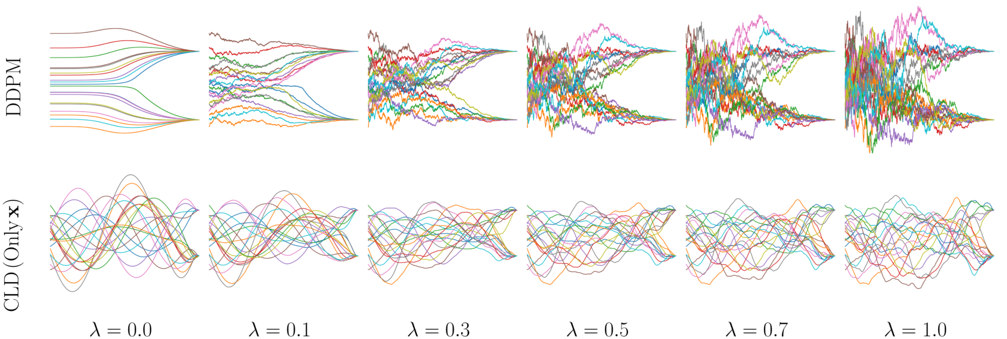
To study the effects of , we visualize the trajectories generated with various but the same random seeds in fig. 5 on our toy example. Clearly, trajectories with smaller have better smoothing property while trajectories with large contain much more randomness. From the fast sampling perspective, trajectories with more stochasticity are much harder to predict with small NFE compared with smooth trajectories.
We include more qualitative results on the choice of and comparison between the Euler-Maruyama (EM) method and the gDDIM in figs. 8 and 9. Clearly, when NFE is small, increasing has a negative effect on the sampling quality of gDDIM. We hypothesize that already generates high-fidelity samples and additional noise may harm the sampling performance. With a fixed number of function evaluations, information derived from score network fails to remove the injected noise as we increase . On the other hand, we find that the EM method shows slightly better quality as we increase . We hypothesize that the ODE or SDEs with small has more oscillations than SDEs with large . It is known that the EM method has a very bad performance for oscillations systems and suffers from large discretization error (Press et al. 2007). From previous experiments, we find that ODE in CLD is highly oscillated.
We also find both methods perform worse than Symmetric Splitting CLD Sampler (SSCS) (Dockhorn et al. 2021) when . The improvement by utilizing Hamiltonian structure and SDEs structure is significant. This encourages further exploration that incorporates Hamiltonian structure into gDDIM in the future. Nevertheless, we also remark that SSCS with performs much worse than gDDIM with .
C.7 More comparisons
We also compare the performance of the CLD model we trained with that claimed in Dockhorn et al. 2021 in table 5. We find that our trained model performs worse than Dockhorn et al. 2021 when a blackbox ODE solver or EM sampling scheme with large NFE are used. There may be two reasons. First, with similar size model, our training scheme not only needs to fit , but also , while Dockhorn et al. 2021 can allocate all representation resources of neural network to . Another factor is the mixed score trick on parameterization, which is shown empirically have a boost in model performance (Dockhorn et al. 2021) but we do not include it in our training.
We also compare our algorithm with more accelerating sampling methods in table 5. gDDIM has achieved the best sampling acceleration results among training-free methods, but it still cannot compete with some distillation-based acceleration methods. In table 6, we compare Predictor-only method with Predictor-Corrector (PC) method. With the same number of steps , PC can improve the quality of Predictor-only at the cost of additional score evaluations, which is almost two times slower compared with the Predictor-only method. We also find large may harm the sampling performance in the exponential multistep method when NFE is small. We note high order polynomial requires more datapoints to fit polynomial. The used datapoints may be out-of-date and harmful to sampling quality when we have large stepsizes.
| Class | Model | NFE () | FID () |
| CLD | our CLD-SGM (gDDIM) | 50 | 2.26 |
| our CLD-SGM (SDE, EM) | 2000 | 2.39 | |
| our CLD-SGM (Prob.Flow, RK45) | 155 | 2.86 | |
| our CLD-SGM (Prob.Flow, RK45) | 312 | 2.26 | |
| CLD-SGM (Prob.Flow, RK45) by Dockhorn et al. 2021 | 147 | 2.71 | |
| CLD-SGM (SDE, EM) by Dockhorn et al. 2021 | 2000 | 2.23 | |
| Training-free Accelerated Score | DDIM by Song et al. 2020a | 100 | 4.16 |
| Gotta Go Fast by Jolicoeur-Martineau et al. 2021b | 151 | 2.73 | |
| Analytic-DPM by Bao et al. 2022 | 100 | 3.55 | |
| FastDPM by Kong & Ping 2021a | 100 | 2.86 | |
| PNDM by Liu et al. 2022 | 100 | 3.53 | |
| DEIS by Zhang & Chen 2022 | 50 | 2.56 | |
| DPM-Solver by Lu et al. 2022 | 50 | 2.65 | |
| Rescaled 2 Order Heun by Karras et al. 2022 | 35 | 1.97 | |
| Training-needed Accelerated Score | DDSS by Watson et al. 2022 | 25 | 4.25 |
| Progressive Distillation by Salimans & Ho 2022 | 4 | 3.0 | |
| Knowledge distillation by Luhman & Luhman 2021 | 1 | 9.36 | |
| Score+Others | LSGM by Vahdat et al. 2021 | 138 | 2.10 |
| LSGM-100M by Vahdat et al. 2021 | 131 | 4.60 | |
| Diffusion GAN by Xiao et al. 2021 | 4 | 3.75 |
| FID at different steps | |||||
| Method | 20 | 30 | 40 | 50 | |
| 0 | Predictor | 16.74 | 9.73 | 6.32 | 5.17 |
| 1 | Predictor | 8.03 | 4.26 | 3.27 | 2.67 |
| PC | 6.24 | 2.36 | 2.26 | 2.25 | |
| 2 | Predictor | 3.90 | 2.66 | 2.39 | 2.32 |
| PC | 3.01 | 2.29 | 2.26 | 2.26 | |
| 3 | Predictor | 332.70 | 292.31 | 13.27 | 2.26 |
| PC | 337.20 | 313.21 | 2.67 | 2.25 | |
C.8 Negative log likelihood evaluation
Because our method only modifies the score parameterization compared with the original CLD (Dockhorn et al. 2021), we follow a similar procedure to evaluate the bound of negative log-likelihood (NLL). Specifically, we can simulate probability ODE eq. 7 to estimate the log-likelihood of given data (Grathwohl et al. 2018). However, our diffusion model models the joint distribution on test data and augmented velocity data . Getting marginal distribution from is challenging, as we need integrate for each . To circumvent this issue, Dockhorn et al. 2021 derives a lower bound on the log-likelihood,
where denotes the entropy of . We can then estimate the lower bound with the Monte Carlo approach.
Empirically, our trained model achieves a NLL upper bound 3.33 bits/dim, which is comparable with 3.31 bits/dim reported in the original CLD (Dockhorn et al. 2021). Possible approaches to further reduce the NLL bound include maximal likelihood weights (Song et al. 2021), and improved training techniques such as mixed score. For more discussions of log-likelihood and how to tighten the bound, we refer the reader to Dockhorn et al. 2021.
C.9 Code licenses
We implemented gDDIM and related algorithms in Jax. We have used code from a number of sources in table 7.
| URL | Citation | License |
|---|---|---|
| https://github.com/yang-song/score_sde | Song et al. 2020b | Apache License 2.0 |
| https://github.com/nv-tlabs/CLD-SGM | Dockhorn et al. 2021 | NVIDIA License |
| https://github.com/qsh-zh/deis | Zhang & Chen 2022 | Unknown |


