Bayesian calibration of coupled computational mechanics models under uncertainty based on interface deformation

We assume that we have a computational forward model $\mathfrak{M}\left({\boldsymbol{x}},C\right)$ for a real-world process, i.e., in our case a single- or multi-field continuum mechanical problem, whose response depends on the choice of inputs ${\boldsymbol{x}}$ and the choice of (e.g., spatio-temporal) coordinates $C$. In general, observations are compared in more than one location and point in time and therefore the coordinates are written as a matrix $C$ with vector entries for each comparison. Consequently, the observations for all coordinates are a matrix $Y_{\mathrm{obs},C}$ as well with vector entries for each coordinate vector. In our case for the comparison of interface deformations, the observations are locations of the interface that define its shape for one or more points in time. The input parameters ${\boldsymbol{x}}$ are the quantities of interest in the calibration process. The vector ${\boldsymbol{x}}$ denotes a collection of model parameters that are subject to calibration and might represent, e.g., material parameters, boundary or initial conditions. The observed data $Y_{\mathrm{obs},C}$ might additionally be subject to unknown measurement noise.

In the Bayesian framework, the calibration problem is interpreted as an update of a prior belief about the parameters, encoded by a prior density $p\left({\boldsymbol{x}}\right)$, by a so-called likelihood model $p\left(Y_{\mathrm{obs},C}|\mathfrak{M}\left({\boldsymbol{x}},C\right)\right)$. The likelihood model expresses the probability density to observe the experimental data $Y_{\mathrm{obs},C}$ at coordinate $C$ given a specific choice of model with input ${\boldsymbol{x}}$ evaluated at the same coordinates $C$. As the expression $p\left(Y_{\mathrm{obs},C}|\mathfrak{M}\left({\boldsymbol{x}},C\right)\right)$ is only a valid density in $Y_{\mathrm{obs},C}$ but not in the model inputs ${\boldsymbol{x}}$ one mostly refers to it as the so-called likelihood function (see section 2.3 for more details). The likelihood function relates the output $\mathfrak{M}\left({\boldsymbol{x}},C\right)$ of the computational model $\mathfrak{M}$ with the observation $Y_{\mathrm{obs},C}$, given a specific choice of parameters ${\boldsymbol{x}}$. The value of $p\left(Y_{\mathrm{obs},C}|\mathfrak{M}\left({\boldsymbol{x}},C\right)\right)$ at a specific ${\boldsymbol{x}}$ can be interpreted as the probability density of the observations $Y_{\mathrm{obs},C}$ for the given model choice $\mathfrak{M}\left({\boldsymbol{x}},C\right)$ or as a score value for the parameter choice ${\boldsymbol{x}}$. The product of the likelihood function and the prior can be evaluated point-wise in the parameter space $\Omega_{{\boldsymbol{x}}}$, yielding a function that we call the unnormalised posterior $p\left(Y_{\mathrm{obs},C}|\mathfrak{M}\left({\boldsymbol{x}},C\right)\right)p\left({\boldsymbol{x}}\right)$. Normalizing this expression by $\int p\left(Y_{\mathrm{obs},C}|\mathfrak{M}\left({\boldsymbol{x}},C\right)\right)p\left({\boldsymbol{x}}\right)\mathrm{d}{\boldsymbol{x}}$ such that we get a valid density that integrates to one, yields the posterior distribution $p\left({\boldsymbol{x}}|Y_{\mathrm{obs},C}\right)$. The posterior distribution can be interpreted as an updated prior distribution, after the knowledge of the experimental data $Y_{\mathrm{obs},C}$ has been incorporated and related to the forward model $\mathfrak{M}\left({\boldsymbol{x}},C\right)$.

An advantage of the Bayesian viewpoint on calibration is the possibility to encode prior knowledge of the unknown parameters or inputs ${\boldsymbol{x}}$ in the so-called prior distribution $p\left({\boldsymbol{x}}\right)$. Prior knowledge is information about the parameters that is available before seeing the data. Often, at least a vague understanding about which values are possible or realistic is available (e.g., the Young’s modulus must be positive $E>0\,\mathrm{Pa}$). This knowledge and additional valuable expert knowledge can be incorporated as prior and therefore the solution of the calibration complies with it.

We can then pose the calibration problem as a Bayesian inference task by applying Bayes’ rule [17]

In (1), the posterior $p\left({\boldsymbol{x}}|Y_{\mathrm{obs},C}\right)$ represents the unique solution of the Bayesian calibration task in the form of a probability density. It is a probability distribution over the input parameters ${\boldsymbol{x}}$ assigning a probability density to each input vector of how well the forward model $\mathfrak{M}\left({\boldsymbol{x}},C\right)$ evaluated with that model parameter combination represents the observation. The interest of the analyst is to find high posterior values and learn for which inputs they occur. The posterior density is usually not known in closed form, due to the implicit dependency on ${\boldsymbol{x}}$ in the forward model $\mathfrak{M}\left({\boldsymbol{x}},C\right)$ within the likelihood function. Nevertheless, the posterior density can be evaluated point-wise, which implies a forward simulation run for the particular choice of ${\boldsymbol{x}}$.

For computationally expensive models, a grid-based evaluation of the posterior in the entire input space $\Omega_{{\boldsymbol{x}}}$ is unfeasible. Due to the curse of dimensionality, this problem becomes especially amplified for $\dim{({\boldsymbol{x}})}\gg 1$. The numerical approximation of the posterior is hence usually conducted using more advanced algorithms which aim to exploit regions in the input space with high posterior density. In this work, we use the sequential Monte Carlo (SMC) method for this purpose but postpone a more detailed discussion of that algorithm and its numerical realization to section 3 and specifically section 3.1, to first focus on the continuous presentation of the Bayesian calibration problem.

The denominator $\int p\left(Y_{\mathrm{obs},C}|\mathfrak{M}\left({\boldsymbol{x}},C\right)\right)p\left({\boldsymbol{x}}\right)\mathrm{d}{\boldsymbol{x}}$, respectively evidence in (1) acts as a normalizing constant for the posterior, such that it becomes a valid density function in ${\boldsymbol{x}}$ which integrates to one on $\Omega_{{\boldsymbol{x}}}$. Nevertheless, the evidence is mostly not computed explicitly, as it involves potentially high dimensional integration over $\Omega_{{\boldsymbol{x}}}$. Consequently, most numerical algorithms operate on the unnormalized posterior or its logarithm and take care of the normalization in an easier to compute post-processing step (see section 3.1). Given the posterior distribution or a numerical representation in form of samples or an approximating distribution, further statistics or point estimates can be calculated and derived.

After the basic concepts of Bayesian calibration have been presented, we want to extend the ideas to the case of non-controllable, uncertain conditions that influence the model $\mathfrak{M}$. Those are summarized in the vector $\boldsymbol{\theta}$. We assume that $\boldsymbol{\theta}$ is not part of the model input variables ${\boldsymbol{x}}$ that we want to calibrate. Instead, it represents inherently uncertain external conditions, e.g., of the experimental set-up, that we cannot fully control at the time of the analysis. Furthermore, we assume that these conditions are subject to uncertainties expressed by a distribution $p\left(\boldsymbol{\theta}\right)$ and that the computational forward model is also dependent on $\boldsymbol{\theta}$ in the sense of $\mathfrak{M}\left({\boldsymbol{x}},\boldsymbol{\theta},C\right)$.

The calibration problem under uncertainty can then be formulated in two steps [18, 19]. First, we naively compose a Bayesian calibration problem in analogy to (1), with the only difference that the model is also dependent on $\boldsymbol{\theta}$. Consequently, the posterior $p\left({\boldsymbol{x}}|\boldsymbol{\theta},Y_{\mathrm{obs},C}\right)$ is conditionally dependent on $\boldsymbol{\theta}$, as demonstrated in (3a). In a second step, we can then average over the effect of the uncertain conditions $\boldsymbol{\theta}$ by taking the expectation of the previous posterior ${\mathbb{E}}_{\boldsymbol{\theta}}\left[p\left({\boldsymbol{x}}|\boldsymbol{\theta},Y_{\mathrm{obs},C}\right)\right]$ with respect to the density $p\left(\boldsymbol{\theta}\right)$ as shown in (3b). The resulting modified posterior, which accounts for the average effect of the additional uncertainty introduced by $\boldsymbol{\theta}$ is then denoted by $q\left({\boldsymbol{x}}|Y_{\mathrm{obs},C}\right)$ and is different from the former posterior $p\left({\boldsymbol{x}}|Y_{\mathrm{obs},C}\right)$ which did not incorporate these additional uncertainties.

Another interpretation of (3b) is the marginalization of the extended posterior $p\left({\boldsymbol{x}},\boldsymbol{\theta}|Y_{\mathrm{obs},C}\right)$ with respect to the uncertain conditions $\boldsymbol{\theta}$. Later-on, we show that the sequential Monte Carlo (SMC) algorithm allows simple operations on the unnormalized extended posterior, analogous to the unnormalized posterior from (1) if no additional uncertainties are present. SMC offers the possibility to conduct the necessary marginalization of $\boldsymbol{\theta}$ as a cheap post-processing step.

The evaluation of the likelihood function, respectively conditional density $p\left(Y_{\mathrm{obs},C}|\mathfrak{M}\left({\boldsymbol{x}},\boldsymbol{\theta},C\right)\right)$ represents the computationally expensive part of the Bayesian calibration as a forward simulation run has to be conducted for every evaluation of the likelihood with respect to $\mathfrak{M}\left({\boldsymbol{x}},\boldsymbol{\theta},C\right)$. The likelihood is a probabilistic model for the discrepancy $\mathfrak{D}$ between experimental data $Y_{\mathrm{obs},C}$ and forward model output $\mathfrak{M}\left({\boldsymbol{x}},\boldsymbol{\theta},C\right)$, written as $\mathfrak{D}=\mathfrak{D}(Y_{\mathrm{obs},C},\mathfrak{M}\left({\boldsymbol{x}},\boldsymbol{\theta},C\right))$. It usually models the statistical behavior of experimental noise and modeling errors. It returns the probability density of the experimental data for a given choice of simulation model. This means that it is centered around the forward model results. Usually, only one experiment is observed.

While many different likelihood models exist [20, 21], we chose the common case of a conditionally independent Gaussian likelihood model with static noise-variance $\sigma_{\mathrm{N}}^{2}$. This choice implies that we assume that the scattering of the measured data $Y_{\mathrm{obs},C}$ can be well-explained by a normal distribution which is centered around the simulation output $Y_{C}$ with variance $\sigma_{\mathrm{N}}^{2}$. Here conditional independence means that the measured noise in $y_{\text{obs},c_{1}}$ does not influence the noise in $y_{\text{obs},c_{2}}$, with $c_{1}$ and $c_{2}$ being two different coordinates.

The conditionally independent Gaussian static likelihood model is given by

wherein $n$ is the dimension of the measurement $Y_{\mathrm{obs},C}$. In the simplest case it is the total number of individual measurements. As most inverse iterators (see section 3) operate on the logarithm of the densities for better numerical condition, we also provide the logarithmic version of (4), which is often abbreviated by $\mathcal{L}({\boldsymbol{x}},\boldsymbol{\theta})$ resulting in

In selecting a likelihood model the immediate question arises about how to define a discrepancy measure $\mathfrak{D}$ between the forward model and experimental results. This becomes especially intricate when the experimental images do not provide real displacements for individual material points, i.e., in this sense prohibit a point-wise correspondence of the geometrical objects. This constraint almost only allows for comparisons of edges, boundaries and interfaces in the image data that can usually be identified depending on their contrast. This step is called segmentation of the image data. More detailed information on segmentation approaches etc. are out of scope for this work. As a result of the segmentation process one obtains a geometric representation of interfaces between different subdomains in the images.

In the following, we present three different discrepancy measures that can be used when working with such kind of image data, namely Euclidean distance at measurement points, closest point projection distance and reproducing kernel Hilbert space norm. Figure 1 shows sketches of the discussed distance measure definitions in 2D. The sketches in Figure 1 are related to the type of problem, of fluid-biofilm interaction, exemplarily analyzed in the numerical examples in section 4. The methods are not bound to this type of problem and can be applied to different topologies or isolated shape characteristics.

An efficient approach is needed to approximate the unnormalized posteriors of the Bayesian calibration problem (1), (3b) and their normalization. While a grid-based approximation of the posterior is feasible for low dimensional parameters $\boldsymbol{x}$, the necessary amount of grid-based evaluations grows exponentially with the dimension of $\boldsymbol{x}$ and SMC methods become significantly more efficient as they exploit regions of high density. Sequential Monte Carlo (SMC) methods are popular sampling methods to efficiently explore a probability distribution $\pi$ for which no closed expression exists.

The result of the SMC sampler is a particle representation $\delta_{{\boldsymbol{x}}^{\left(i\right)}}$ of $\pi$ with associated weights $w^{\left(i\right)}$ in the form of

Therein every particle has a location and weight $\left\{{\boldsymbol{x}}^{\left(i\right)},w^{\left(i\right)}\right\}_{i=1}^{N}$. It is further known [33, 34] that with this approximation any integral over an integrable function $h\left({\boldsymbol{x}}^{\left(i\right)}\right)$ can be approximated by a sum that converges to the integral

Specifically, we use an SMC method [35] which sequentially blends over from a particle representation of a predefined prior distribution to a particle representation of the actual posterior distribution. A convenient aspect of the particle representation in (12) is that they allow for a straightforward approximation of integrals (13), as they appear in marginal distributions (2). This is especially useful for Bayesian calibration under uncertainty and the associated integration in (3b). Here, the numerical integration is conducted by simply ignoring the dependency on $\boldsymbol{\theta}$ in the particle representation.

The SMC algorithm we use in this work uses an adaptive step length based on [36, 33, 34]. Herein, a control parameter $\zeta$ for the effective sample size (ESS) is used to control step length. The ESS is defined as

and is a measure for the current weight distribution. The ESS represents how well the probability density mass is distributed amongst the used particles.

The presentation of the SMC algorithm is compactly demonstrated in the pseudo-algorithm Algorithm 1 and described in remark 5. For more details, the interested reader is referred to [29, 30, 34].

The so-called tempering strategy that defines the transition from the prior to the posterior as a sequence is written as

with the logarithmic likelihood $\mathfrak{L}\left({\boldsymbol{x}}\right)$ as introduced in (5) and the prior $p\left({\boldsymbol{x}}\right)$. Finally, after reaching $\gamma=1$ the particle approximation has blended over into one for the posterior distribution.

To efficiently evaluate the likelihood function in (15) we use a Gaussian process (GP) regression model [39] for the log-likelihood function (5) that can be trained on a controllable amount of forward model evaluations. The main idea is that for a given computational budget, represented by the number of forward model runs, the approximation error of the surrogate is considerably smaller than the error in the SMC posterior approximation for the same number of forward simulation runs. A similar approach, where the model output is directly used as data to train a Gaussian process regression model as a surrogate for Bayesian calibration was used in [1]. Gaussian processes are often used to generate regression models and therefore a brief summary of the core equations is presented in appendix D. The presented overall approach would also work with different regression approaches as linear or spline interpolation or in case of cheap enough forward models would also work directly on the forward model.

We use the log-likelihood $\mathfrak{L}\left({\boldsymbol{x}}\right)$ of the Bayesian calibration problem as presented in (5) to train our GP upon. This gives the advantage that the regression models do not need to fulfill positiveness constraints. This would be the case if the GP was trained on the unnormalized posterior or likelihood directly. Another advantage of learning the log-likelihood function in contrast to learning the simulation response is that the log-likelihood is a scalar function.

Training data $\mathcal{D}$ are input-output pairs of values that are known about the process and the regression model can be based on. In our case, we can evaluate the forward model with any choice of model parameters ${\boldsymbol{x}}$, compare it to the observed experiment and determine the logarithm of the log-likelihood $\boldsymbol{\mathfrak{L}}$ (5). To simplify notation we specify the training data outputs to a vector of log-likelihoods $\boldsymbol{\mathfrak{L}}_{\mathrm{train}}$ at different coordinates ${\boldsymbol{x}_{\mathrm{train}}}$. Thus, we are free to choose any input batch ${\boldsymbol{x}_{\mathrm{train}}}$ and compute resulting output $\boldsymbol{\mathfrak{L}}_{\mathrm{train}}$ according to our computational budget. The generation of the training data $\mathcal{D}$ for the Gaussian process regression causes the highest computational costs in the inverse analysis, as for every training tuple $\{\mathfrak{L}_{\text{train},i},\boldsymbol{x}_{\text{train},i}\}$ one forward model evaluation is required, due to the dependency of the log-likelihood (5) on the forward model.

Some further advantages of the surrogate approach are an a priori controllable amount of simulation runs, which can also be conducted in parallel, in contrast to the batch-sequential model evaluations that the SMC would impose on the forward model evaluations in a direct application. Once the surrogate is generated, the SMC algorithm can run without the risk of encountering non-converging or failing forward simulations.

To generate the training data $\mathcal{D}$ we choose a space-filling design strategy, namely a quasi-random Sobol sequence [40, 41]. The Sobol sequence has the advantage to have superior uniformity properties [42] and additionally allows for generating further sequential points that still share the space filling properties.

The implementation of the algorithm described above was done in the Python software framework QUEENS [43]. Herein, the Gaussian process regression module GPy [44] was used for the construction of the Gaussian process surrogates. The sequential Monte Carlo algorithm based on Algorithm 1 is also implemented in QUEENS. For processing of forward model results the Python package vtk for ”The Visualization Toolkit” was used [45]. Some of the following visualizations were generated with Seaborn [46] and Matplotlib [47]. Parallel axis plots are generated with plotly [48]. We furthermore use PyTorch [49] for the generation of the Sobol sequences. The forward models were solved with the in-house C++ research code BACI [50].

The calibration is performed for hyperelastic material properties of the solid domain for which we will calibrate the two parameters of a Saint-Venant Kirchhoff material model. For the given setup of FSI models for biofilms and the biofilm flow cell data, the location of the fluid-biofilm interface is the primary data available and therefore used for comparison. A schematic sketch of the problem setup is drawn in Figure 2. For easier demonstration we first investigate a two-dimensional calibration problem ($\dim(\boldsymbol{x})=2$) without experimental uncertainties ($\dim(\boldsymbol{\theta})=0$) and then move on to more complex examples.

We chose the same problem setup as presented in [12]. The biofilm geometry is inspired by analyses done on experimental results in [11, 14]. The model domain represents a two-dimensional channel with dimensions $1\,\mathrm{mm}\times 2\,\mathrm{mm}$, where horizontal fluid flow with parabolic profile is enforced from the left boundary (see $\Gamma^{\mathrm{F}}_{\mathrm{in}}$ in Figure 2) with a maximal volume rate of $\dot{V}_{\mathrm{in}}=100\,{\mathrm{mm^{2}}/\mathrm{s}}$. The solid biofilm (green) is attached to the channel floor. A no-slip condition for the fluid is used on the channel floor and top boundary as well as the biofilm on the channel floor (see $\Gamma^{\mathrm{F}}_{\mathrm{D}}$ and $\Gamma^{\mathrm{S}}_{\mathrm{D}}$ in Figure 2) and a horizontal outflow is enforced on the right edge (see $\Gamma^{\mathrm{F}}_{\mathrm{out}}$ in Figure 2). These boundary conditions are modeled via Dirichlet boundary conditions on the fluid velocity (and solid displacement accordingly) and respective free outflow in horizontal direction. The horizontal condition represents the ongoing empty channel left and right from the modeled domain.

To generate the artificial experimental data, we use a forward simulation of the fluid-biofilm interaction with a Saint-Venant-Kirchhoff material model for the solid biofilm domain. The material is characterized by two parameters, namely Young’s modulus $E$ and Poisson’s ratio $\nu$. We summarize the chosen input parameters, used for the generation of the data, in form of the ground truth vector ${\boldsymbol{x}}_{\mathrm{gt}}=\begin{bmatrix}\nu=0.3,E=400\,\mathrm{Pa}\end{bmatrix}^{\mathsf{T}}$. The fluid has a dynamic viscosity of $\mu^{{\mathrm{F}}}=10^{-3}\,\mathrm{Pa\,s}$ and a density of $\rho^{{\mathrm{F}}}=10^{3}\,{\mathrm{kg}/\mathrm{m^{3}}}$ as a model for water. The biofilm has the same density as the fluid. The solution of the velocity and pressure field of the fluid and displacement field of the biofilm is depicted in Figure 3 for the regarded quasi-steady deformed state in the ground truth forward model evaluation. As a reaction to the load imposed by the fluid inflow boundary condition, the solid bends towards the right as it is plotted in Figure 4. In Figure 4a we see the artificial observation data $Y_{\mathrm{obs},C}$ as the result of the reference simulation with ground truth values ${\boldsymbol{x}}_{\mathrm{gt}}$. $Y_{\mathrm{obs},C}$ represents the deformed location (green) of the interface in this example for one single point in time $C$. In Figure 4b we plot the results for some exemplary parameter combinations additionally.

In a first step, we compare the effect of the different discrepancy measures as introduced in section 2.4. We directly approximate the log-likelihood by the posterior mean function of a Gaussian process surrogate and use the discussed discrepancy measures. Additionally, we also provide the posterior standard deviation of the GP to quantify the remaining uncertainty in the surrogate. All surrogate models for the log-likelihood function resulting for the different discrepancy measures use the same training input that was sampled with a quasi-random Sobol sequence to yield a space-filling training design (see section 3.2). The training inputs are different parameters in the forward model and the resulting forward simulations.

For an estimation of a suitable $\sigma_{\mathrm{N}}$ in the likelihood model (4) the known resolution $\approx 8\,\mathrm{\mu m}$ of OCT [14, 15] is considered. The noise standard deviation is assumed to be in the same order of magnitude, such that $\sigma_{\mathrm{N}}=0.01\,\mathrm{mm}$ is used in the following. OCT resolution and standard deviation in the likelihood model are not expected to be equal. A further discussion is omitted here, as the demonstration here works independent of the choice and an expressive value can only be found related to real data and chosen image segmentation. For the RKHS norm we need two parameters $\sigma_{\mathrm{N}}$ and $\sigma_{\mathrm{W}}$. An estimation of the length scale $\sigma_{\mathrm{W}}$ for the RBF kernel in the RKHS approach in (10b) is made as $\sigma_{\mathrm{W}}=0.005\,\mathrm{mm}$, being approximately $10\%$ of the maximal displacement magnitude (see Figure 3a).

The resulting regression models for the likelihoods are shown in Figure 5 for $n_{\mathrm{train}}=1000$ training points with a Matérn 3/2 kernel (see appendix D, eq. 27 for details). In general, the likelihood over the parameters can be understood as a score value of how well the forward model response with respective parameters leads to similar results compared to the reference data. A discussion and interpretation of the figure will follow below. For this first comparison, we just use this large number of training points and postpone the discussion on the GP convergence over $n_{\mathrm{train}}$ to the case only using the RKHS norm measure. For the distribution of the measurement points in this comparison, the reader is referred to [12]. In Figure 5 the fields of the likelihoods are determined from the logarithmic likelihoods and those fields are normalized in the plots for better comparability. Parameter combinations that led to failed forward model evaluations are marked by gray crosses in the following figures. For our setup, the failing simulations occurred for low values of Young’s modulus (located on the left side of the plots) representing soft biofilm material, which lead to large mesh distortions in the ALE FSI approach. For the sake of comparability, the respective logarithmic likelihoods are plotted in Figure 6 and the associated standard deviations in the regression models in Figure 7.

It can be seen, that the response in the likelihoods show a high likelihood of the parameters in red for a characteristic curved shape with its peak at the expected ground truth parameters ${\boldsymbol{x}}_{\mathrm{gt}}=\begin{bmatrix}\nu=0.3,&E=400\,\mathrm{Pa}\end{bmatrix}^{\mathsf{T}}$. A high likelihood corresponds to a high probability density of the parameter combination to represent the reference data. This means that the corresponding values for ${\boldsymbol{x}}$ in this region of the input space result in simulation outputs that are very close to the observation data under the employed discrepancy measure. The likelihood falls very close to zero when moving away from the high likelihood regions, representing low similarity of the forward model result compared to the reference data. Especially the failed simulations (gray crosses) fall in a region with very low likelihood values which renders them irrelevant for our investigations. For the rest of the input space, it can be seen in Figure 7 that the standard deviation in the regression model is low and only rises in regions with little data.

Comparing the Euclidean distance measure in Figure 5a and the closest point projection in Figure 5b it can be seen, that the second one is more peaked around the maximum of the likelihood that is close to the ground truth value ${\boldsymbol{x}}_{\mathrm{gt}}$. This is also a consequence of the formulation (4) and (5), as the numbers of distance measurements differ greatly with the number of measurement points ${n_{\mathrm{\mathrm{mp}}}}=10$ and the number of interface nodes ${n_{\mathrm{in}}}=66$. The higher number of individual single point measurements generally leads to a more peaked likelihood with the same $\sigma_{\mathrm{N}}$. It must also be stated that no further weighting of the closest point projection distances was done, so all nodal closest point projection distances are considered equally important. This includes the distances for many mesh nodes, that are close to the boundary conditions and therefore there the displacement magnitude is lower. An additional data compression approach, e.g., kernel principal component analysis [21, 52] or also a selection of only a subset of the interface nodes could be used to increase comparability, but this is outside of the scope of the current article. The likelihood from the RKHS based distance measure (in Figure 5c) combines both features to be expressive around the maximum likelihood (ML) point and still have information from more distant points. The RKHS norm measure correlates all discretized interface locations and orientations of the model to all counterparts in the observation (see (11)), therefore it is also expected to be the most detailed measure for this comparison.

The likelihood based on the forward model evaluations adequately combined with prior distributions results in the posterior (see (1)), which is a probability density of the parameters leading to the observations. It is favorable to have an expressive posterior and therefore expressive likelihood as a result to be able to compare posterior values for different parameter combinations and with that develop an understanding of the forward model in relation to the observations. In the case of a very flat likelihood the conclusion is that all parameter combinations are similarly well suited to explain the observations and therefore they are potentially insignificant to the forward model, at least in the range of the regarded parameter intervals. This means that all input parameters ${\boldsymbol{x}}$ will lead to forward model results that are very close to the observation under the employed discrepancy measure. The expressive shape of the likelihood based on the RKHS based measure underlines that this measure is well suitable in the given example to be used for Bayesian calibration. Therefore it is used in all following examples.

The presented likelihoods were generated using the different discrepancy measures (6), (7) and (11) and all yield similar characteristics in the shape of the likelihood. Therefore it can be concluded that in this setting and a fluid-biofilm interface-based measurement of a flow cell experiment an underestimation of Young’s modulus $E$ is coupled to an underestimation of Poisson’s ratio $\nu$. In applications with real experimental data, it would make sense to restrict the training points to the intervals, that are believed to contain the optimum or at least relevant values for the parameters. That could mean to restrict the Poisson’s ratio to positive values, as this is what would be expected for most materials. Nevertheless, the resulting shapes representing high likelihood are very smooth for the whole tested range between $\nu=-0.8$ and $\nu=0.5$ and do not show a distinct border between positive and negative values. This is interesting with regard to biofilm mechanics in flow cell experiments as it shows that the estimation of $E$ and $\nu$ is coupled for all surface comparisons that were tested. For some investigations, this also hints toward the need to incorporate additional measurements or information, e.g., prior knowledge.

The most costly part of the presented algorithm are the forward model evaluations that are necessary to generate the training data $\mathcal{D}$ of the GP log-likelihood regression model. While the convergence of the GP over the number of training data points is dependent on the character of the underlying function as well as on the selected design of experiments, we want to show a short qualitative convergence study for the problem at hand for the distance measure based on the RKHS inner product. In general the convergence study of a GP w.r.t. the number of training points is difficult as usually it is not feasible to increase the data point set size by orders of magnitude. Therefore other strategies, e.g., leave-one-out cross validation can be used as a proxy for the regression error [39]. The requirement towards the number of training points and the regression model is to catch the relevant shape characteristics of the likelihood.

For the application of such an approach, it is crucial to know how many forward model evaluations are required to get results efficiently. To get a first picture the Gaussian process regression model for the logarithmic likelihood is created for a series of training point set sizes $n_{\mathrm{train}}$. For this qualitative study, only the RKHS norm based likelihood was used as it uses the most detailed comparison and seems to give the most expressive shape of the posterior. The likelihood parameters were set to $\sigma_{\mathrm{W}}=0.005\,\mathrm{\mu m}$, $\sigma_{\mathrm{N}}^{2}=0.0005\,\mathrm{mm}^{2}$ in all following examples. The choice $\sigma_{\mathrm{N}}^{2}=0.0005\,\mathrm{mm}^{2}$ in our case relates to the discretization size, as the rounded squared average interface element length is $\bar{l}^{2}\approx 0.0005\mathrm{mm}^{2}$. It is difficult to interpret $\sigma_{\mathrm{N}}$ in relation to the measurement error alone, as especially also the image segmentation approach chosen to determine the model fluid-biofilm interface from experimental data influences the choice. We deviated from this parameter choice for $\sigma_{\mathrm{N}}$ in the comparison of the measures to keep it the same for all measures.

We used a Matérn 2/3 kernel (see appendix D, eq. 27) with one length scale hyperparameter $l$ (in the standardized input space) and one signal variance $\sigma_{0}^{2}$ which will be determined via ML estimation using an L-BFGS-B optimizer for the evidence of the GP (see eq. 29). The Matèrn 2/3 kernel appeared to be the best suitable to represent the likelihood field as it resulted for the given example. Especially the great variety in steepness and therefore low smoothness of the likelihood seems to be the challenge for the regression approach. However, at the moment, no general recommendation for the GP kernel can be given. As commonly done [39] we used a fixed nugget noise $\sigma_{\mathrm{n}}^{2}=10^{-5}\cdot\left(\mathrm{max}\left(\boldsymbol{\mathfrak{L}}_{\mathrm{train}}\right)-\mathrm{min}\left(\boldsymbol{\mathfrak{L}}_{\mathrm{train}}\right)\right)$ to stabilize the training of the GP.

In the following, the convergence of the likelihood surrogate model over the number of used training points is qualitatively shown for the problem at hand. For this study, the Sobol sequence sampling property is used as all samples are consecutive samples from the same Sobol sequence. In Figure 8 it is apparent, that only very few training points are necessary to estimate the general shape of the likelihood distribution and have a rough estimate for the optimum. With $n_{\mathrm{train}}=200$ samples the ML estimate is already in good agreement with the ground truth ${\boldsymbol{x}}_{\mathrm{gt}}=\begin{bmatrix}\nu=0.3,&E=400\,\mathrm{Pa}\end{bmatrix}^{\mathsf{T}}$.

It can be concluded that for this two-dimensional example the likelihood surrogate shows relevant features and the global shape well for $n_{\mathrm{train}}=200$ forward model evaluations and no significant gain in accuracy can be expected for a moderate increase of the sample size. Given that in the following examples a comparison with different priors is made and another problem dimension in form of an uncertain parameter is added, and therefore the complexity is increased, we use the Gaussian process model with one length scale for all (standardized) parameters, a fixed nugget noise and $n_{\mathrm{train}}=1000$ training points for the following examples (see Remark 6 on dimensionality).

In this subsection, the regression model will be generated according to the findings in the previous examples. The GP was constructed with a Matérn 2/3 kernel, a single length scale and signal variance for all parameters and a fixed nugget noise variance $\sigma_{\mathrm{n}}^{2}$ in (29). 1000 samples were used for the training of the GP. As the likelihood model is available in form of a cheap to evaluate surrogate, we use 5000 SMC particles and 20 rejuvenation steps per SMC iteration (which would result in 1 million likelihood calls for 10 SMC iterations). For the adaptive step size of the SMC iterator a control parameter of $\zeta=0.995$ was used (see Algorithm 1).

In the following examples, we examine the influence of priors in the parameters and uncertainties on the resulting posteriors. In Figure 9 all results discussed in this section are plotted on the same page for better comparability. The different cases will be described and discussed subsequently in the following paragraphs. Figure 9 displays the resulting posteriors of the examples in form of SMC particle approximations. To visualize the character of the data, one particle distribution is shown explicitly in Figure 9b, where the particles are plotted at their respective coordinates. The particle weights are illustrated as circle size and in a color scale. The other three subplots (Figure 9a, Figure 9c and Figure 9d) show two-dimensional hexagonal histograms in a color scale. The particles are sorted into the displayed bins and summed up using their weights. The percentiles of the two-dimensional posteriors are additionally simplified as kernel density estimates (KDE) that are shown as black solid lines. For the KDE a radial basis function (RBF) kernel with bandwidth optimization was used.

On the top and right sides, the marginal distributions depending on both individual input parameters are plotted as histograms. The one-dimensional marginal posterior distributions $p\left(E|Y_{\mathrm{obs},C}\right)$ and $p\left(\nu|Y_{\mathrm{obs},C}\right)$ can easily be approximated by sorting the weighted particles into bins in the respective dimension. The marginals are additionally displayed in form of KDEs as black solid lines. The used priors are indicated as red dashed lines in all following plots.

Characteristic points deduced from the particle approximation are marked as crosses. The maximum a posteriori (MAP) estimate ${\boldsymbol{x}}_{\mathrm{MAP}}$ is marked in green and the posterior mean (PM) ${\boldsymbol{x}}_{\mathrm{PM}}$ in orange.

In high dimensions, the posterior cannot be plotted as easily as in the two-dimensional case. The analyst wants to have a comparative overview of where the mean value of the posterior is and how the probability mass is distributed in the posterior. For that and as another common approximation, we also show percentile lines of the global Gaussian approximation to the posterior in orange. The global Gaussian approximation is parameterized by the posterior mean (PM) vector ${\boldsymbol{x}}_{\mathrm{PM}}$ and the covariance matrix which can both be calculated from the weighted SMC particles very quickly.

We also present the Laplace approximation [21] of the posterior distribution around the MAP estimate depicted in Figure 9a and Figure 9c with green solid lines for the two cases without uncertainty. The Laplace approximation can be understood as a local quadratic approximation of the posterior density function around its MAP in the log space in form of a Gaussian distribution. The covariance matrix of the resulting local Gaussian distribution gives an idea of how fast the posterior changes in a certain direction, starting from the MAP estimate. Please note, that the posterior distribution is not known in closed form but only approximated by SMC particles with associated weight. We approximate the MAP estimate by the SMC particle that scored the highest posterior value in the last rejuvenation step of the last iteration. In these examples, the necessary gradients of the posterior distribution were approximated by finite differences w.r.t. the input variables ${\boldsymbol{x}}$ on the GP regression model. The Laplace approximation was omitted for the case with uncertain inflow. Laplace approximations are used for approximative Bayesian inverse analysis methods [6], where the MAP is first found through optimization and then the Lagrange approximation is computed for an estimate of the variance.

In our last example we want to calibrate material properties of a heterogeneous biofilm FSI model as in [12], but here under an uncertain inflow rate boundary condition. Heterogeneity comes into play in such problems due to different age and/or different nutrient availability of different parts of the domain. Hence, it was a natural choice to also shed some light on a more demanding case involving more parameters. The three subdomains are depicted in Figure 12 and lead to six input parameters, consisting of the Young’s modulus and Poisson’s ratio of each subdomain.

The parameters ${\boldsymbol{x}}_{\mathrm{gt}}=[E_{1}=500\,\mathrm{Pa},\;\nu_{1}=0.2,\;E_{2}=200\,\mathrm{Pa},\;\nu_{2}=0.1,\;E_{3}=1000\,\mathrm{Pa},\;\nu_{3}=0.3]^{\mathsf{T}}$ for a hyperelastic Saint-Venant-Kirchhoff material model are used as the ground truth inputs, along with the inflow rate $\dot{V}_{\mathrm{in}}=100\,{\mathrm{mm^{2}}/\mathrm{s}}$. All other model details are the same as for the previous examples, to then generate the synthetic experimental data $Y_{\mathrm{obs},C}$ for this heterogeneous case. Please note that in this example we additionally assume noise polluted measurement data according to

For the following example we choose noise with a standard deviation of $\sigma_{\text{n,obs}}=1\,\mathrm{\mu m}$. In remark 9 we comment on the determination of the GP surrogate for this example.

For the SMC approach a set of 10000 particles with 30 rejuvenation steps was used with a step size control parameter of $\zeta=0.998$. Just as a comparison to the $n_{\mathrm{train}}=2000$ training points used, a full evaluation in every rejuvenation step of the SMC algorithm would require three million ($10000\cdot 30\cdot 10=3000000$) forward model evaluations for exemplary 10 SMC steps. This is neither desirable nor feasible if directly applied to the expensive forward model. After the proof of concept in previous examples, with two input parameters and potentially one uncertain parameter, it must be emphasized, that volume integrals for respective marginals and especially the normalization of the posterior (1) in six plus one dimensions scale even worse. Just for a moderately sized, grid-based discretization with 100 sample points in every dimension we would get $100^{7}$ necessary evaluations of the GP-mean. So we make use of the good scalability of the SMC algorithm in higher dimensions in the following examples.

As already indicated above, in this last example we want to show the full capability of the approach and therefore we use an example with uncertain inflow rate $\dot{V}_{\mathrm{in}}$ and added noise to the data generated from the ground truth values. The assumed distribution on $\dot{V}_{\mathrm{in}}$ is the same as in Figure 10 above with a beta-distribution $\mathcal{B}\left(\dot{V}_{\mathrm{in}}|a=2.6,b=1.4\right)$ between $0\,{\mathrm{mm^{2}}/\mathrm{s}}$ and $110\,{\mathrm{mm^{2}}/\mathrm{s}}$ with its mode at $88\,{\mathrm{mm^{2}}/\mathrm{s}}$. The MAP approximation is found at ${\boldsymbol{x}}_{\mathrm{MAP}}=[E_{1}\approx 345\,\mathrm{Pa},\;\nu_{1}\approx 0.43,\;E_{2}\approx 135\,\mathrm{Pa},\;\nu_{2}\approx 0.30,\;E_{3}\approx 1034\,\mathrm{Pa},\;\nu_{3}\approx-0.47]^{\mathsf{T}}$ and the global posterior mean computes to ${\boldsymbol{x}}_{\mathrm{PM}}=[E_{1}\approx 443\,\mathrm{Pa},\;\nu_{1}\approx-0.15,\;E_{2}\approx 431\,\mathrm{Pa},\;\nu_{2}\approx-0.13,\;E_{3}\approx 637\,\mathrm{Pa},\;\nu_{3}\approx-0.14]^{\mathsf{T}}$. Analogously to the lower dimensional example, the MAP estimate is obtained with a binning approach with 10 intervals in each input dimension. Therefore it is a rough estimate. Nevertheless, the curse of dimensionality inhibits an excessively fine grid. The maximum of the posterior under uncertainty qualitatively represents the ground truth with $E_{3}>E_{1}>E_{2}$ and $\nu_{1}>\nu_{2}$. Only for $\nu_{3}$, it does not correspond to the ground truth. This can be a consequence of the relevance of the parameter to the overall posterior, as the lateral contraction in the stiffest subdomain, attached to the ground also has little effect on the interface deformation. In challenging examples it can be a good idea to first perform a global sensitivity analysis [54, 55] and then focus the inverse analysis only on the most sensitive parameters. It also shows again, that the problem setup is challenging as the volume inflow rate is used as an uncertain parameter. But this is also often the case in real-world applications. This has the effect that the MAP parameters are those of a less stiff biofilm material, than the ones used for the ground truth simulation.

The resulting one dimensional marginals over the parameters, for which uniform priors were assumed, are plotted in Figure 13 as histograms with KDE approximations in black. Here the letter $q({\boldsymbol{x}}|Y_{\mathrm{obs},C})$ is used because the distributions represent marginals of the posterior under uncertainty (3b).

It can be observed that most of these marginals show a rather uniform distribution. In this example, this happens as they represent the integration of the posterior with respect to all other parameters respectively and therefore the probability mass is accumulated herein. Only for subdomain $\Omega_{2}$ (in Figure 13c and Figure 13d) the posterior marginals acummulate density around the ground truth $E_{2}\approx 200\,\mathrm{Pa}$ and $\nu_{2}>0$. As these single-dimensional marginals are not unveiling the full complexity of the posterior, a further step is made to show two-dimensional marginals for a selected combination of parameters in Figure 14 as hexagonal histograms with the percentile lines of the KDE approximations. Therein the interaction effects between the respective combination of parameters can be seen. Especially within the regions enclosed by the percentile lines of $10\%$ the most probable parameter combinations for the respective marginals can be found.

The marginal posterior distributions in Figure 14 show complex densities. As compared to a deterministic calibration approach for the same example [12], where even the less complex case with a fixed volume inflow rate $\dot{V}_{\mathrm{in}}$ could not be solved, this complex character can be well represented here in the obtained solution. Furthermore, for Figure 14a and Figure 14c it can be seen that $E_{2}$ dominates the marginal posteriors that are high around $E_{2}\approx 200\,\mathrm{Pa}$ for a plausible range of the other Young’s moduli $E_{1},E_{3}$. Also the shape of the distribution for $\Omega_{2}$ in Figure 14e resembles the posterior shape in Figure 9d, which is the one for homogeneous example with uniform prior and uncertain inflow. This means that parameters in $\Omega_{2}$ qualitatively have similar influence in this marginal, as the two parameters have in the homogeneous example in the posterior. This is also expected as $\Omega_{2}$ takes up the highest portion of the biofilm domain (see Figure 12) and therefore dominates the deformation.

As we have six parameters involved, a full plot of the posterior is impossible. Alternatively, a parallel axis plot as in Figure 15 can be used to get an idea of the underlying posterior shape.

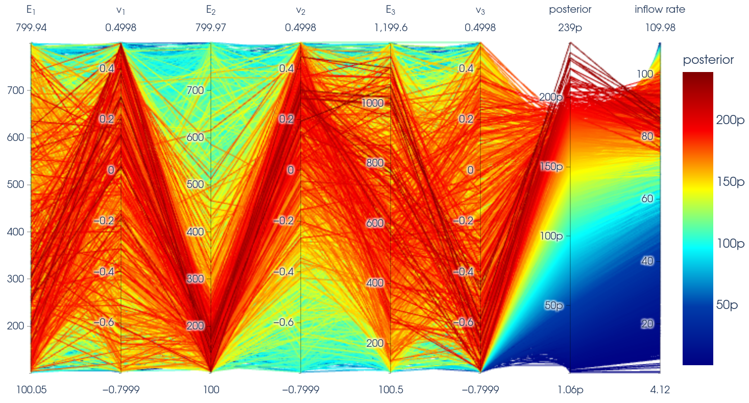
Over the first six axis we see the input parameters for the range of interest. The seventh axis shows the extended posterior values for the 10000 particles from the SMC particle approximation. The last axis represents the uncertain inflow boundary condition $\dot{V}_{\mathrm{in}}$. Every line connecting the axis represents one particle of the SMC solution and all lines are colored by their absolute extended posterior density value. The lines are drawn on top of each other, starting with low posterior density values in blue and ending with the highest ones in red. Most of the parameter combinations with high posterior density accumulate around $E_{2}\approx 200\,\mathrm{Pa}$ and $\nu_{1},\nu_{2}>0$. The other three parameters $E_{1},E_{3},\nu_{3}$ seem to score relatively high posterior values for the whole range of interest. That means they are individually less significant to a specific value of the posterior density. Given the subdomain topology, as seen in Figure 12, these posterior results can also be expected as $\Omega_{2}$ takes up the largest portion of the biofilm and therefore can also be expected to have the highest influence on the deformation in this case.

The possibility for such a phenomenological interpretation of the posterior is a very attractive feature of tackling the inverse problem via the proposed approach, as not only good point estimates can be concluded, but more importantly the influence of the individual parameters on the posterior can be observed and interpreted. The information revealed in such a probablistic analysis, as for example displayed in Figure 14 and Figure 15, gives indeed a lot of insight into the problem at hand. Among others, it also shows how useful given experimental information is or whether other measurements are needed for the identification of relevant parameters. With the rich information from such an analysis also an estimation of the plausibility and stability of the point estimates can be made. As an example, a deterministic or trial and error approach might end up in identifying negative Poisson ratios for biofilms (easily understandable when looking at Figure 9 or Figure 15) and hence identifying biofilms as auxetic materials, as it has been done in the past. The probabilistic analysis would immediately show the lack of validity for such a conclusion.

References

- [1] I Bilionis and N Zabaras “Solution of inverse problems with limited forward solver evaluations: a Bayesian perspective” In Inverse Problems 30.1 IOP Publishing, 2013, pp. 015004 DOI: 10.1088/0266-5611/30/1/015004
- [2] Marc. Kennedy and Anthony O’Hagan “Bayesian calibration of computer models” In Journal of the Royal Statistical Society: Series B (Statistical Methodology) 63.3 Wiley, 2001, pp. 425–464 DOI: 10.1111/1467-9868.00294
- [3] Albert Tarantola “Inverse Problem Theory and Methods for Model Parameter Estimation” SIAM Society for IndustrialApplied Mathematics, Philadelphia, 2005 URL: https://www.ebook.de/de/product/12013271/albert_tarantola_inverse_problem_theory_and_methods_for_model_parameter_estimation.html
- [4] Philippe Moireau, Dominique Chapelle and Patrick Tallec “Filtering for distributed mechanical systems using position measurements: perspectives in medical imaging” In Inverse Problems 25.3 IOP Publishing, 2009, pp. 035010 DOI: 10.1088/0266-5611/25/3/035010
- [5] M. Sermesant, P. Moireau, O. Camara, J. Sainte-Marie, R. Andriantsimiavona, R. Cimrman, D.L.G. Hill, D. Chapelle and R. Razavi “Cardiac function estimation from MRI using a heart model and data assimilation: Advances and difficulties” In Medical Image Analysis 10.4 Elsevier BV, 2006, pp. 642–656 DOI: 10.1016/j.media.2006.04.002
- [6] Sebastian Kehl and Michael. Gee “Calibration of parameters for cardiovascular models with application to arterial growth” In International Journal for Numerical Methods in Biomedical Engineering 33.5 Wiley, 2016, pp. e2822 DOI: 10.1002/cnm.2822
- [7] Hans-Curt Flemming and Jost Wingender “The biofilm matrix” In Nature Reviews Microbiology 8.9 Springer ScienceBusiness Media LLC, 2010, pp. 623–633 DOI: 10.1038/nrmicro2415
- [8] Markus Böl, Alexander. Ehret, Antonio Albero, Jan Hellriegel and Rainer Krull “Recent advances in mechanical characterisation of biofilm and their significance for material modelling” In Critical Reviews in Biotechnology 33.2 Taylor & Francis, 2013, pp. 145–171 DOI: 10.3109/07388551.2012.679250
- [9] Erin. Gloag, Stefania Fabbri, Daniel. Wozniak and Paul Stoodley “Biofilm mechanics: Implications in infection and survival” In Biofilm 2 Elsevier BV, 2020, pp. 100017 DOI: 10.1016/j.bioflm.2019.100017
- [10] Héloïse Boudarel, Jean-Denis Mathias, Benoı̂t Blaysat and Michel Grédiac “Towards standardized mechanical characterization of microbial biofilms: analysis and critical review” In npj Biofilms and Microbiomes 4 Springer ScienceBusiness Media LLC, 2018, pp. 17 DOI: 10.1038/s41522-018-0062-5
- [11] Cristian Picioreanu, Florian Blauert, Harald Horn and Michael Wagner “Determination of mechanical properties of biofilms by modelling the deformation measured using optical coherence tomography” In Water Research 145 Elsevier BV, 2018, pp. 588–598 DOI: 10.1016/j.watres.2018.08.070
- [12] Harald Willmann and Wolfgang. Wall “Inverse analysis of material parameters in coupled multi-physics biofilm models” In submitted to: Advanced Modeling and Simulation in Engineering Sciences, 2021 arXiv:2110.07200
- [13] Michael Wagner, Danial Taherzadeh, Christoph Haisch and Harald Horn “Investigation of the mesoscale structure and volumetric features of biofilms using optical coherence tomography” In Biotechnology and Bioengineering 107.5 Wiley, 2010, pp. 844–853 DOI: 10.1002/bit.22864
- [14] Florian Blauert, Harald Horn and Michael Wagner “Time-resolved biofilm deformation measurements using optical coherence tomography” In Biotechnology and Bioengineering 112.9, 2015, pp. 1893–1905 DOI: 10.1002/bit.25590
- [15] Luisa Gierl, Kasper Stoy, Andrés Faíña, Harald Horn and Michael Wagner “An open-source robotic platform that enables automated monitoring of replicate biofilm cultivations using optical coherence tomography” In npj Biofilms and Microbiomes 6 Springer ScienceBusiness Media LLC, 2020, pp. 18 DOI: 10.1038/s41522-020-0129-y
- [16] Benjamin. Jackson, James. Connolly, Robin Gerlach, Isaac Klapper and Albert. Parker “Bayesian estimation and uncertainty quantification in models of urea hydrolysis by E. coli biofilms” In Inverse Problems in Science and Engineering 29.11 Informa UK Limited, 2021, pp. 1629–1652 DOI: 10.1080/17415977.2021.1887172
- [17] Christian. Robert “The Bayesian Choice” Springer, New York, 2007 DOI: 10.1007/0-387-71599-1
- [18] Raphael Sternfels and Phaedon-Stelios Koutsourelakis “Stochastic design and control in random heterogeneous materials” In International Journal for Multiscale Computational Engineering 9.4 Begell House, 2011, pp. 425–443 DOI: 10.1615/IntJMultCompEng.v9.i4.60
- [19] P.S. Koutsourelakis “Design of complex systems in the presence of large uncertainties: A statistical approach” In Computer Methods in Applied Mechanics and Engineering 197.49-50 Elsevier BV, 2008, pp. 4092–4103 DOI: 10.1016/j.cma.2008.04.012
- [20] Jari Kaipio and Erkki Somersalo “Statistical and Computational Inverse Problems” Springer New York, 2004 DOI: 10.1007/b138659
- [21] Christopher. Bishop “Pattern Recognition and Machine Learning” Springer-Verlag New York Inc., 2011
- [22] N. Aronszajn “Theory of reproducing kernels” In Transactions of the American Mathematical Society 68.3 American Mathematical Society (AMS), 1950, pp. 337–337 DOI: 10.1090/S0002-9947-1950-0051437-7
- [23] Marc Vaillant, Joan Glaunès, Gary Christensen and Milan Sonka “Surface Matching via Currents” In Information Processing in Medical Imaging Springer Berlin, Heidelberg, 2005, pp. 381–392
- [24] Alexandre Imperiale, Alexandre Routier, Stanley Durrleman and Philippe Moireau “Improving Efficiency of Data Assimilation Procedure for a Biomechanical Heart Model by Representing Surfaces as Currents” In Functional Imaging and Modeling of the Heart Berlin, Heidelberg: Springer Berlin Heidelberg, 2013, pp. 342–351 DOI: 10.1007/978-3-642-38899-6˙41
- [25] Charles Geyer “Practical markov chain monte carlo” In Statistical science JSTOR, 1992, pp. 473–483
- [26] Siddhartha Chib and Edward Greenberg “Understanding the Metropolis-Hastings Algorithm” In The American Statistician 49.4 Taylor & Francis, 1995, pp. 327–335 DOI: 10.1080/00031305.1995.10476177
- [27] Peter. Glynn and Donald. Iglehart “Importance Sampling for Stochastic Simulations” In Management Science 35.11 Institute for Operations Researchthe Management Sciences (INFORMS), 1989, pp. 1367–1392 DOI: 10.1287/mnsc.35.11.1367
- [28] Surya. Tokdar and Robert. Kass “Importance sampling: a review” In WIREs Computational Statistics 2.1 Wiley, 2010, pp. 54–60 DOI: 10.1002/wics.56
- [29] “Sequential Monte Carlo Methods in Practice” Springer New York, 2001 DOI: 10.1007/978-1-4757-3437-9
- [30] Nicolas Chopin and Omiros Papaspiliopoulos “An Introduction to Sequential Monte Carlo” Springer International Publishing, 2020 DOI: 10.1007/978-3-030-47845-2
- [31] David. Blei, Alp Kucukelbir and Jon. McAuliffe “Variational Inference: A Review for Statisticians” In Journal of the American Statistical Association 112.518 Taylor & Francis, 2017, pp. 859–877 DOI: 10.1080/01621459.2017.1285773
- [32] Matthew. Hoffman, David. Blei, Chong Wang and John Paisley “Stochastic Variational Inference” In Journal of Machine Learning Research 14.4, 2013, pp. 1303–1347 URL: http://jmlr.org/papers/v14/hoffman13a.html
- [33] Pierre Del, Arnaud Doucet and Ajay Jasra “Sequential Monte Carlo for Bayesian Computation” In Bayesian Statistics 8, Oxford University Press, 2007, pp. 1–34
- [34] P.S. Koutsourelakis “A multi-resolution, non-parametric, Bayesian framework for identification of spatially-varying model parameters” In Journal of Computational Physics 228.17 Elsevier BV, 2009, pp. 6184–6211 DOI: 10.1016/j.jcp.2009.05.016
- [35] N. Chopin “A sequential particle filter method for static models” In Biometrika 89.3 Oxford University Press (OUP), 2002, pp. 539–552 DOI: 10.1093/biomet/89.3.539
- [36] Pierre Del, Arnaud Doucet and Ajay Jasra “Sequential Monte Carlo samplers” In Journal of the Royal Statistical Society: Series B (Statistical Methodology) 68.3, 2006, pp. 411–436 DOI: 10.1111/j.1467-9868.2006.00553.x
- [37] S.. Minson, M. Simons and J.. Beck “Bayesian inversion for finite fault earthquake source models I—theory and algorithm” In Geophysical Journal International 194.3 Oxford University Press (OUP), 2013, pp. 1701–1726 DOI: 10.1093/gji/ggt180
- [38] Christian. Robert and George Casella “Monte Carlo Statistical Methods” Springer New York, 2004 DOI: 10.1007/978-1-4757-4145-2
- [39] Carl Rasmussen and Christopher.. Williams “Gaussian Processes for Machine Learning” first (University of Cambridge) second (University of Edinburgh) Cambridge, Massachusetts: MIT Press Ltd, 2006
- [40] IM Sobol “The Distribution of Points in a Cube and the Accurate Evaluation of Integrals (in Russian)” In Zh. Vychisl. Mat. i Mater. Phys 7, 1967, pp. 784–802
- [41] Art. Owen “Scrambling Sobol’and Niederreiter–Xing Points” In Journal of Complexity 14.4 Elsevier, 1998, pp. 466–489 DOI: 10.1006/jcom.1998.0487
- [42] Sergei Kucherenko, Daniel Albrecht and Andrea Saltelli “Exploring multi-dimensional spaces: a Comparison of Latin Hypercube and Quasi Monte Carlo Sampling Techniques”, 2015 arXiv:1505.02350
- [43] J. Biehler, J. Nitzler, W.A. Wall and V. Gravemeier “QUEENS – A Software Platform for Uncertainty Quantification, Physics-Informed Machine Learning, Bayesian Optimization, Inverse Problems and Simulation Analytics: User Guide”, AdCoEngineeringGW, 2019
- [44] GPy “GPy: A Gaussian process framework in python” http://github.com/SheffieldML/GPy, Last accessed on 2021-08-20, since 2012
- [45] Will Schroeder, Ken Martin and Bill Lorensen “The visualization toolkit : an object-oriented approach to 3D graphics” Clifton Park, N.Y: Kitware, 2006
- [46] Michael. Waskom “seaborn: statistical data visualization” In Journal of Open Source Software 6.60 The Open Journal, 2021, pp. 3021 DOI: 10.21105/joss.03021
- [47] J.. Hunter “Matplotlib: A 2D graphics environment” In Computing in Science & Engineering 9.3 IEEE COMPUTER SOC, 2007, pp. 90–95 DOI: 10.1109/MCSE.2007.55
- [48] Plotly Technologies Inc. “Collaborative data science” Montreal, QC: Plotly Technologies Inc., 2015 URL: https://plot.ly
- [49] Adam Paszke, Sam Gross, Francisco Massa, Adam Lerer, James Bradbury, Gregory Chanan, Trevor Killeen, Zeming Lin, Natalia Gimelshein, Luca Antiga, Alban Desmaison, Andreas Kopf, Edward Yang, Zachary DeVito, Martin Raison, Alykhan Tejani, Sasank Chilamkurthy, Benoit Steiner, Lu Fang, Junjie Bai and Soumith Chintala “PyTorch: An Imperative Style, High-Performance Deep Learning Library” In Advances in Neural Information Processing Systems 32 Curran Associates, Inc., 2019, pp. 8024–8035
- [50] “BACI: A Comprehensive Multi-Physics Simulation Framework” https://baci.pages.gitlab.lrz.de/website/, Last accessed on 2021-16-06
- [51] Mirella Coroneo, Lena Yoshihara and Wolfgang. Wall “Biofilm growth: A multi-scale and coupled fluid-structure interaction and mass transport approach” In Biotechnology and Bioengineering 111.7 Wiley, 2014, pp. 1385–1395 DOI: 10.1002/bit.25191
- [52] Bernhard Schölkopf, Alexander Smola and Klaus-Robert Müller “Kernel principal component analysis” In Artificial Neural Networks — ICANN’97 1327 Springer Berlin Heidelberg, 1997, pp. 583–588 DOI: 10.1007/BFb0020217
- [53] David Duvenaud “Automatic model construction with Gaussian processes”, 2014
- [54] Sebastian Brandstaeter, Sebastian. Fuchs, Jonas Biehler, Roland. Aydin, Wolfgang. Wall and Christian. Cyron “Global Sensitivity Analysis of a Homogenized Constrained Mixture Model of Arterial Growth and Remodeling” In Journal of Elasticity 145.1-2 Springer ScienceBusiness Media LLC, 2021, pp. 191–221 DOI: 10.1007/s10659-021-09833-9
- [55] Barbara Wirthl, Sebastian Brandstaeter, Jonas Nitzler, Bernhard. Schrefler and Wolfgang. Wall “Global sensitivity analysis based on Gaussian-process metamodelling for complex biomechanical problems”, 2022 arXiv:2202.01503
- [56] Jonas Nitzler, Jonas Biehler, Niklas Fehn, Phaedon-Stelios Koutsourelakis and Wolfgang. Wall “A Generalized Probabilistic Learning Approach for Multi-Fidelity Uncertainty Propagation in Complex Physical Simulations” In submitted to: Computer Methods in Applied Mechanics and Engineering, 2022 arXiv:2001.02892
- [57] Michael Wagner and Harald Horn “Optical coherence tomography in biofilm research: A comprehensive review” In Biotechnology and Bioengineering 114.7 Wiley, 2017, pp. 1386–1402 DOI: 10.1002/bit.26283
- [58] M.. Gee, U. Küttler and W.. Wall “Truly monolithic algebraic multigrid for fluid-structure interaction” In International Journal for Numerical Methods in Engineering 85.8 Wiley, 2010, pp. 987–1016 DOI: 10.1002/nme.3001
- [59] L. Yoshihara, M. Coroneo, A. Comerford, G. Bauer, T. Klöppel and W.. Wall “A combined fluid-structure interaction and multi-field scalar transport model for simulating mass transport in biomechanics” In International Journal for Numerical Methods in Engineering 100.4 Wiley, 2014, pp. 277–299 DOI: 10.1002/nme.4735
- [60] U. Küttler, M. Gee, Ch. Förster, A. Comerford and W.. Wall “Coupling strategies for biomedical fluid-structure interaction problems” In International Journal for Numerical Methods in Biomedical Engineering 26.3-4 Wiley, 2010, pp. 305–321 DOI: 10.1002/cnm.1281
- [61] Danial Taherzadeh, Cristian Picioreanu, Ulrich Küttler, Angelo Simone, Wolfgang. Wall and Harald Horn “Computational study of the drag and oscillatory movement of biofilm streamers in fast flows” In Biotechnology and Bioengineering 105.3 Wiley, 2010, pp. 600–610 DOI: 10.1002/bit.22551
- [62] Alain Berlinet and Christine Thomas-Agnan “Reproducing Kernel Hilbert Spaces in Probability and Statistics” Springer US, 2004 DOI: 10.1007/978-1-4419-9096-9
- [63] Michael. Stein “Interpolation of Spatial Data” Springer New York, 1999
- [64] B. Matérn “Spatial Variation” Springer New York, 1986 DOI: 10.1007/978-1-4615-7892-5