Toward a new theory of the fractional quantum Hall effect
Abstract
The fractional quantum Hall effect was experimentally discovered in 1982. It was observed that the Hall conductivity of a two-dimensional electron system is quantized, , in the vicinity of the Landau level filling factor . In 1983, Laughlin proposed a trial many-body wave function, which he claimed described a “new state of matter” – a homogeneous incompressible liquid with fractionally charged quasiparticles. Here I develop an exact diagonalization theory that allows calculation of the energy and other physical properties of the ground and excited states of a system of two-dimensional Coulomb interacting electrons in a strong magnetic field. I analyze the energies, electron densities, and other physical properties of the systems with electrons, continuously as a function of magnetic field in the range . The results show that both the ground and excited states of the system resemble a sliding Wigner crystal, whose parameters are influenced by the magnetic field. Energy gaps in the many-particle spectra appear and disappear as the magnetic field changes. I also calculate the physical properties of the Laughlin state for and show that neither this state nor its fractionally charged excitations describe the physical reality. The results obtained shed new light on the nature of the ground and excited states in the fractional quantum Hall effect.
I Introduction
I.1 Historical background
The quantum Hall effect was discovered by Klaus von Klitzing in 1980 von Klitzing et al. 1980. He studied the longitudinal () and Hall () resistances of a degenerate two-dimensional (2D) electron gas (EG) in the inversion layer of a Si-MOSFET (metal-oxide-semiconductor field effect transistor). The sample was placed in a strong perpendicular magnetic field T and cooled down to K. The resistances and were measured as a function of the gate voltage , applied between the metallic gate and the 2DEG, which changed the density of 2D electrons and the Landau level filling factor
| (1) |
here
| (2) |
is the cyclotron frequency, and is the effective mass of electrons ( is the magnetic length). He found that, when is close to integer values , , the diagonal resistance becomes negligibly small, while the Hall resistance takes on, with a very high accuracy, quantized values, corresponding to the Hall conductivity
| (3) |
The origin of this fascinating physical phenomenon, which was called the integer quantum Hall effect, was quickly understood von Klitzing et al. 1980 in terms of the single-particle picture. The Landau quantization of electron motion leads to the appearance of energy gaps in the electron spectrum when ; the classical formula for the Hall conductivity , together with the relation (1) immediately gives the quantized values (3). The stabilization of at the levels (3) and the vanishing of in finite intervals around was explained by the influence of disorder, see, e.g., Ref. Prange and Girvin 1990.
The time of mysteries came a little later. In 1982 Tsui, Stormer and Gossard published a paper Tsui et al. 1982 where the same transport coefficients ( and ) were measured in another material system, GaAs/AlGaAs heterojunction. The main difference between the new experiment and the one of von Klitzing was that the mobility of 2D electrons was higher ( cm2/Vs) and the temperature was lower ( down to K). In the experiment Tsui et al. 1982 the density of electrons was fixed while the magnetic field varied from zero up to T. Like in Ref. von Klitzing et al. 1980, the already familiar integer quantization of was observed around , but – very surprisingly – a very similar plateau was found around , where the measured corresponded to the Hall conductivity
| (4) |
Subsequent experimental studies showed that such a fractional quantization of and the corresponding suppression of is the case around many fractions of the form where and are integers and is odd, as well as around some fractions with an even denominator, see, e.g., Ref. Willett et al. 1987.
If , all electrons occupy the highly degenerate lowest Landau level, and there are no energy gaps in the single-particle electron spectrum. Therefore the mysterious feature at could be explained only within a many-body approach, taking into account electron-electron interactions. As known, when considered as classical point particles, Coulomb-interacting electrons form the Wigner crystal Wigner 1934, and Tsui et al. Tsui et al. 1982 put forward a hypothesis that the observed feature in the Hall conductivity is related to the formation of the Wigner crystal (or a charge density wave) with a triangular symmetry. However, in 1983 Laughlin Laughlin 1983a proposed the following trial wave function for the ground state of the -particle system at :
| (5) |
where LS means the “Laughlin state”, is odd integer, , and are the normalized complex coordinates of 2D electrons. The function is an eigenfunction of the total angular momentum operator with the eigenvalue (in units of ). If , it coincides with the wave function of the so called maximum density droplet (MDD) state proposed earlier in Ref. Bychkov et al. 1981 for the ground state of the system at . The MDD state is characterized by a uniform electron density at , see Section V for further details.
For and the energy of the states (5) in the thermodynamic limit was evaluated in Ref. Laughlin 1983a, and it was found that it is lower than the energy of the charge density wave calculated in Refs. Yoshioka and Fukuyama 1979; Yoshioka and Lee 1983 using the Hartree-Fock Yoshioka and Fukuyama 1979 and second-order perturbation theory Yoshioka and Lee 1983. The projections of and onto the numerically calculated exact ground states for three and four particles were also calculated and found to be close to 1. Apart from the function (5) Laughlin also “generated” many-body wave functions for elementary excitations of the system and stated that they describe quasiparticles with fractional charge . Finally he concluded that the wave function (5) describes the ground state of the system at and is “an incompressible quantum fluid with fractionally charged excitations” Laughlin 1983a. A few critical comments on the wave function (5) followed Tao 1984, and several more attempts to find an alternative ground state of the fractional quantum Hall effect (FQHE) system Maki and Zotos 1983; Yoshioka et al. 1983 have been made, but finally the LS (5) was accepted by the community NP9 as the closest approximation to the ground-state wave function at (with and 5). Laughlin’s ideas have been developed in a very large number of subsequent publications, see, e.g., Refs. Girvin and Jach 1983; Haldane 1983; Levesque et al. 1984; Jain 1989; Kasner and Apel 1994; Tsiper and Goldman 2001; Morf et al. 2002; Wan et al. 2002; Wan et al. 2003; Ciftja and Wexler 2003; Ciftja et al. 2004; Ciftja et al. 2011 and review articles Eisenstein and Stormer 1990; Girvin 2004; Jain 2012; Hansson et al. 2017; Murthy and Shankar 2003. In order to explain the fractions different from , various theoretical approaches have been proposed, for example, hierarchical schemes Haldane 1983 or the composite fermions theory Jain 1989. According to the currently accepted version of the FQHE theory, based on the theory Laughlin 1983a, a 2D electron system placed in a strong magnetic field undergoes a sequence of phase transitions at various fractional values of into highly idealized dissipationless states Girvin 2004. Reports on the experimental observations of fractionally charged quasiparticles were published in Refs. Goldman and Su 1995; Saminadayar et al. 1997; de-Picciotto et al. 1997.
I.2 Brief overview of results of this work
In this paper, I develop an exact diagonalization theory that enables calculation of the energy and other physical properties of the ground and excited states of two-dimensional Coulomb interacting electrons placed in a strong magnetic field. It is assumed that all electrons are spin-polarized and occupy only the lowest Landau level states. It is also assumed that the electrons are in the field of a neutralizing positively charged background, which has the shape of a disk of radius and constant surface density . I present exact results for the ground and excited states of the systems of electrons, both for and for arbitrary varying from to , in dependence of the magnetic field . The results show that electron-electron and background-electron interactions lift the degeneracy of the Landau levels and lead to the appearance of energy gaps in the many-body spectra of the FQHE system. As the magnetic field changes, the width of the energy gaps oscillates, remaining on order of in finite intervals of the magnetic field and disappearing at separate -points. The oscillations of the gap width are caused by the interplay of the Coulomb repulsive forces and the compressive action of the field. Both the ground and excited states of the FQHE system have a shape reminiscent of a Wigner crystal (or a Wigner molecule) in the sense that the electron density maxima are in the same places where one would expect to find Coulomb interacting point charges. All these results shed new light on the true nature of the ground and excited states of the 2D electron systems in strong magnetic fields and lead to a better understanding of the FQHE effect.
A large part of this paper is devoted to a detailed analysis of the currently accepted theory of this phenomenon. I investigate physical properties of the state (5) for , as well as of its “fractionally charged” excitations, and show that they have no relation to the true ground and excited states of the FQHE system. The results obtained in this work force the conclusion that the Laughlin liquid with its fractionally charged excitations does not exist.
It should be noted that, although the currently accepted FQHE theory claims that the Laughlin function well describes the properties of the system in the thermodynamic limit, no precise evidence for such statements has been presented. Moreover, it is obvious that such evidence cannot exist, since in order to obtain it, it would be necessary to solve the many-body Schrödinger equation for a very large number of () strongly interacting particles. On the other hand, some exact results have been obtained in the literature for systems with a small number of particles, see, e.g., exact diagonalization calculations of Ref. Kasner and Apel 1994 (for and ) and of Ref. Tsiper and Goldman 2001 (for and ). Although the results of these exact calculations have been found in clear contradiction with the variational theory of Ref. Laughlin 1983a, the Laughlin theory was not questioned. In Ref. Kasner and Apel 1994 the discrepancies were ignored, while in Ref. Tsiper and Goldman 2001 a complicated and questionable interpretation in terms of an edge reconstruction of the LS into a “chiral striped phase” was put forward. I discuss these and some other statements of the currently accepted FQHE theory in Sections VI.7 and VIII below.
The rest of the paper is organized as follows. In Section II I formulate the problem and discuss all the technical issues needed for the remaining part of the paper; in particular, the many-particle matrix elements of the Hamiltonian and other physical quantities are calculated there. In Section III the classical solution of the problem, the Wigner crystal, is briefly discussed. In Section IV results of the exact solution of the problem for and up to particles are presented. Then I switch to a discussion of the LS. In Section V I overview the physical properties of the MDD state () which are used in the subsequent discussion of the FQHE problem. In Section VI the energy and other physical properties of the trial state (5) for and are calculated and compared with the exact results from Section IV.
After the complete analysis of the case , I present in Section VII the results of the exact solution of the problem for . In Section VIII a number of statements of the currently accepted FQHE theory are analyzed and discussed, and finally in Section IX all results of this work are summarized and conclusions are formulated. Mathematical details are given in the Appendices.
II Theory
II.1 Single-particle problem
Let us consider a single 2D electron moving in the plane in the presence of a uniform external magnetic field . Its quantum-mechanical motion is described by the single-particle Schrödinger equation
| (6) |
Its solution,
| (7) |
| (8) |
is characterized by the radial quantum number and the azimuthal (angular momentum) quantum number . The functions (8) represent a complete basis set in a 2D space.
The states with and non-positive , , belong to the lowest Landau level. The corresponding energy equals and the corresponding wave functions are
| (9) |
where , and . The states (9) are normalized, , and represent a complete subset of functions in two dimensions belonging to the lowest Landau level with . The matrix elements of the exponential function between the single-particle states (9) are
| (10) |
where is the polar angle of the vector , , and are the Laguerre polynomials.
II.2 Positive background
electrons repel each other by Coulomb forces, therefore a compensating positive background is required to keep them together and to ensure the system electroneutrality. I will use two physically reasonable models of the positive background density. The first model, also used, for example, in Refs. Laughlin 1983a; Ciftja and Wexler 2003; Ciftja et al. 2004; Ciftja et al. 2011, assumes that the positive background has the shape of a disk with a uniform charge density and a radius ,
| (11) |
Here , is the Heaviside step function, and the length is defined as
| (12) |
In the second model, the density profile is smoothed near the disk edge at the length ,
| (13) |
where is the Euler Gamma function, is the incomplete Gamma function, and
| (14) |
is the regularized incomplete Gamma function. The smooth density profile (13) actually gives a more adequate description of the real density distribution, since in real systems the edge is always smeared over a certain length, for example, over the distance between the 2D gas and the donor layer in GaAs/AlGaAs heterostructures or over the average distance between electrons . The length , defined in (12), will be used as the length unit throughout the paper. In contrast to other possible options for choosing the length unit (e.g., or , as was done in many publications), does not depend on , which is more convenient for the system behavior analysis at varying magnetic fields, see Section VII.
The both density profiles, (11) and (13), satisfy the condition
| (15) |
and are shown in Figure 1 for . The Fourier transforms of the density profiles (11) and (13) are determined by the formulas
| (16) |
and
| (17) |
respectively, where is the Bessel function, and are the Laguerre polynomials.

The potential well created by the positively charged background disk with the density (11) or (13) is described by the formula
| (18) |
where
| (19) |
for the step-like density profile (11), and
| (20) |
for the smooth density profile (13). Here the functions and , defined as
| (21) |
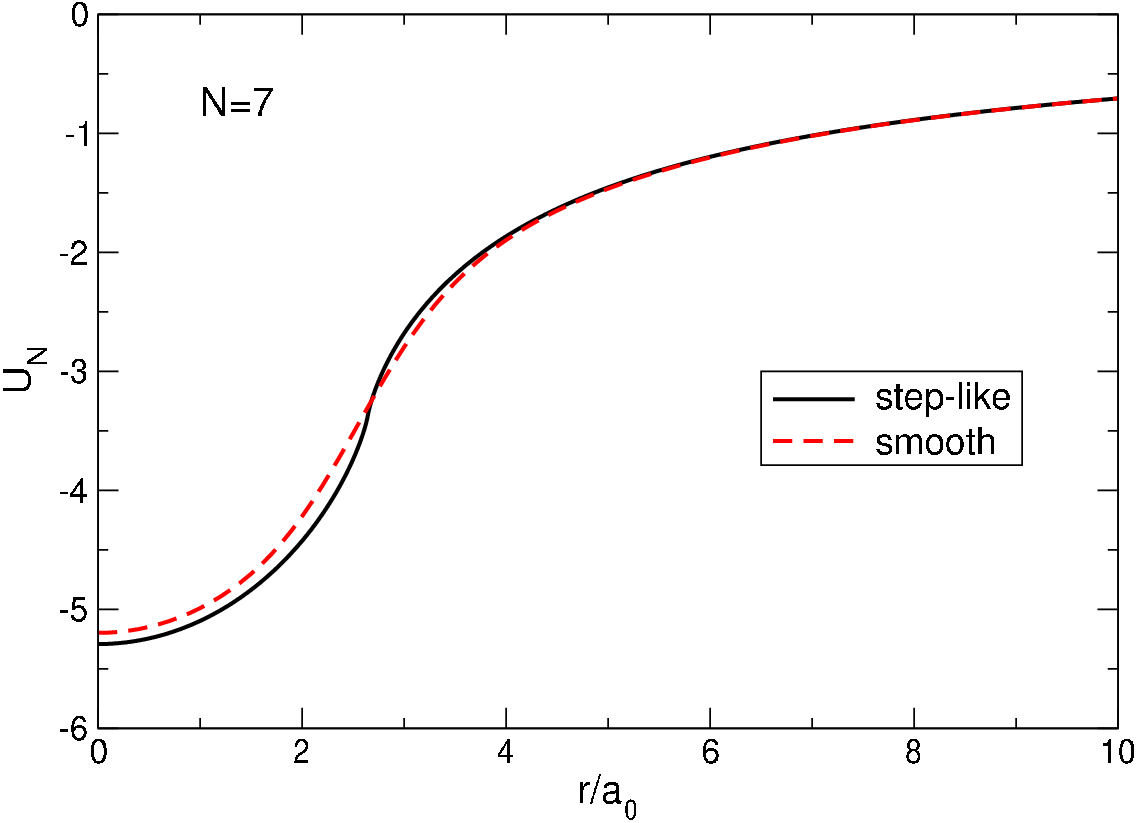
are complete elliptic integrals of the first and second kind, respectively, are the binomial coefficients, is the Gamma function, and is the degenerate (confluent) hypergeometric function, Eq. (155). Figure 2 shows the functions (19) and (20) for . In the case of the step-like density profile, the potential well is slightly deeper, while in the case of the smooth density profile, it is slightly wider. The depths of both potential wells grow with as , . In real, macroscopically large samples () this depth is on the keV scale.
II.3 Many-body Hamiltonian
The Hamiltonian of interacting 2D electrons, placed in the magnetic field and in the attractive potential (18) of the positively charged background with the density (11) or (13), has the form
| (22) |
Here is the total kinetic energy operator and the Coulomb interaction energy consists of the sum of background-background, background-electron and electron-electron interaction energies,
| (23) |
In order to calculate the energy it is convenient to rewrite (23) in terms of Fourier transforms of the electron and background charge densities. This gives
| (24) |
where are given by Eqs. (16) and (17), for the step-like and smooth density profiles respectively. The Hamiltonian (22) commutes with the total angular momentum operator
| (25) |
The total angular momentum quantum number can be used to classify the many-body basis wave functions.
II.4 Basis many-body wave functions
Let us consider spin-polarized electrons at the lowest Landau level. Each of the particles can occupy one of the states (9). If the -th particle is in the single-particle state , the corresponding many-body wave function can be written as a Slater deteminant
| (26) |
The functions (26) are orthogonal and normalized,
| (27) |
They are eigenfunctions of the kinetic energy operator
| (28) |
and of the total angular momentum operator
| (29) |
where the latter is measured in units of . The many-body wave functions (26) represent the orthonormal basis set of functions belonging to the lowest Landau level.
If electrons occupy the single-particle states with the lowest possible angular momenta from up to , one gets the many-body configuration , Ref. Bychkov et al. 1981, which is often referred to as the maximum density droplet (MDD) state. This MDD configuration has the lowest possible total angular momentum
| (30) |
If , there exist, in general, more than one many-body electronic configurations corresponding to the given and . For example, Tables 1 and 2 show possible many-body configurations for and and several ’s. The number of many-body configurations grows with for a given .
| Configurations | ||
|---|---|---|
| 1 | 1 | |
| 2 | 1 | |
| 3 | 2 | |
| 4 | 2 | |
| 5 | 3 | |
| 6 | 3 | |
| 7 | 4 |
| Configurations | ||
|---|---|---|
| 3 | 1 | |
| 4 | 1 | |
| 5 | 2 | |
| 6 | 3 | |
| 7 | 4 | |
| 8 | 5 | |
| 9 | 7 | |
| 10 | 8 | |
| 11 | 10 | |
| 12 | 12 |
II.5 Many-body matrix elements
To calculate various physical properties of an -electron system one needs matrix elements of one-particle or two-particle operators,
| (31) |
| (32) |
with the many-body states (26). In this paper, only the matrix elements (31)–(32) between the many-body states and that belong to the same total angular momentum will be needed, i.e., . This means that, if the bra and ket configurations are different, they differ by two or more single-particle states. For example, the configurations and , and differ by two single-particle states, while the configurations and differ by three single-particle states, see Table 2. The matrix elements between the bra and ket configurations which differ by only one single-particle state, e.g., between the configurations and , will not be considered since they correspond to different values of the total angular momentum .
Now I calculate matrix elements of several one-particle and two-particle operators of the type (31)–(32). For brevity, the short notations for the functions (26) will be used.
II.5.1 Electron density
II.5.2 Fourier transform of the electron density
II.5.3 Background-background interaction energy
The background-background interaction energy is given by the first term in Eq. (24). Since does not depend on the coordinates of electrons, the matrix is diagonal and all matrix elements are the same. For the step-like (11) and smooth (13) density profiles they are given by the following formulas
| (37) |
| (38) |
where the integrals are defined and calculated in Appendix A, see Eqs. (142) and (143).
II.5.4 Background-electron interaction energy
The background-electron interaction energy is given by the second term in Eq. (24). Its many-body matrix elements are
| (39) |
Substituting the Fourier transforms of the background and electron densities from Eqs. (16), (17), and (36) into (39) I obtain the following results. In the case of the step-like density profile calculations give (for details see Appendix B.1)
| (40) |
where
| (41) |
is the inverse Landau level filling factor. In the case of the smooth density profile the results are expressed it terms of the integral (Appendix A)
| (42) |
The matrix elements (40) and (42) depend on the magnetic field .
II.5.5 Electron-electron interaction energy
The electron-electron interaction energy is given by the third term in Eq. (24). Calculating its many-body matrix elements I get the following result
| (43) |
where the diagonal matrix elements are given by the difference of Hartree and Fock contributions,
| (44) |
| (45) |
Substituting here the matrix elements of the exponential functions from Eq. (10) I get
| (46) |
| (47) |
where the integrals are related to the integrals defined above, see Appendix A, and in the last formula
| (48) |
The formulation of results for the off-diagonal matrix elements () requires a bit longer discussion. First, since , the sets of numbers and , , differ from each other. In general, these sets may differ by one, two or more numbers. The case when they differ by only one number is excluded, as explained above. If they differ by more than two numbers, the corresponding matrix elements equal zero,
| (49) |
Thus, the matrix elements are nonzero if and only if the states and differ from each other by the single-particle states of exactly two particles. For example, for three particles with the total angular momentum , Table 2, the matrix elements
| (50) |
are finite (only two numbers in the bra and ket configurations are different), but the matrix element
| (51) |
is zero (all three numbers are different).
Let the configurations
| (52) |
differ from each other by the -states of exactly two particles. I designate them as , and , , and their serial numbers in the sets and as , , , ; all other states in (52), designated by dots, are identical. For example, for the first of the matrix elements in (50), , these numbers are , , , , and , , , . For the second matrix element in (50), , they are , , , , and , , , .
Now one can formulate the results for the off-diagonal matrix elements of the electron-electron interaction energy. Calculations show that for
| (53) | |||||
where the integrals are defined in Eq. (144).
Equations (43), (46), (47) and (53) give the matrix elements of the electron-electron interaction between the basis many-body configurations (26). Note that the magnetic field enters these formulas only via the common prefactor , which means that for all values of the -interaction matrix needs to be calculated only once.
II.5.6 Pair correlation function
The operator of the pair correlation function is defined as
| (54) |
Its diagonal and off-diagonal matrix elements are determined by the following formulas,
| (55) |
| (56) |
where the numbers , , , , as well as , , , have the same meaning as in the previous Section.
II.6 General solution of the many-body Schrödinger problem
Let us consider the -particle Schrödinger equation
| (57) |
In order to solve it for a given total angular momentum , the function should be searched in the form of a linear combination of all many-body configurations corresponding to given values of and ,
| (58) |
In this formula are unknown numbers. Substituting (58) into (57) and multiplying the resulting equation by one reduces the Schrödinger problem to the matrix equation
| (59) |
The size of the Hamiltonian matrix here is . Solving the eigenvalue problem (59) one can find solutions for given and : the energies and the sets of numbers , , which give the corresponding many-body wave functions according to the expansion (58). After the numbers are found one can also calculate all physical properties of the ground or excited many-body states, for example, the electron density and the pair correlation function, using the corresponding matrix elements found in Section II.5.
All matrix elements of the Hamiltonian are calculated analytically, see Section II.5. As a result, the energies and the wave functions of the -electron system can be calculated, in principle, with a very high accuracy for any and any and . In practice, the computation time becomes too large if or are much greater than one, but the ground state physics of a FQHE system can be well understood even if the number of particles is less than or on the order of ten. Especially valuable are results for , because seven spin-polarized electrons form a highly symmetric piece of a macroscopic Wigner crystal, see Figure 3(g) below.
In Section IV I present results of the theory for and the Landau level filling factor . Before doing so, however, it is useful to discuss the purely classical solution of the problem.
III Wigner crystal
The physics of the considered system is determined by the interplay of attractive forces acting on electrons by the positively charged background, and the inter-electron Coulomb forces repelling them from each other. If () classical point charges are placed in the attractive potential of the positive background they may form two types of Wigner molecules (at small ), Fig. 3: with a single shell, when all particles are located on a ring of a finite radius , Figs. 3(a)–3(e), and with two shells, when one particle is at the center of the positively charged disk, and particles are located on a ring around the center, Figs. 3(f)–3(h). I will denote these two configurations as and , respectively. To understand which of the two possibilities is actually the case, one should calculate the total energy of the Wigner molecules in both situations.


The potential energy of the positively charged background disk is described by Eqs. (18)–(19) for the step-like density profile and by Eqs. (18), (20) for the smooth density profile. The both potential energies are shown in Figure 2. In the single-shell configuration the (dimensionless) complex coordinates of electrons can be written as
| (60) |
with being the shell radius. Then the total energy of the system is
| (61) |
where are given either by (19) or by (20), and
| (62) |
In the two-shell Wigner molecule , the particle coordinates are
| (63) |
and the total energy has the form
| (64) |
Minimizing the energies (61) and (64) with respect to one can find the radii of the shells , for both types of molecules and both types of the density profiles, and their total energies. The results of such calculations are shown in Tables 3 and 4 for the step-like and smooth density profiles. One sees that for both density profiles the energy of the configuration is smaller than that of the configuration, if . The opposite inequality, , is valid at and . If , the energies of both configurations are very close to each other: in the case of the step-like density profile (11) the two-shell configuration has a slightly lower energy, with a difference of %. In the case of the smooth density profile (13) the one-shell configuration has a slightly lower energy, with a difference of %. Thus the classical solution of the problem has rotational symmetry of order , where
| (65) |
in the case of the step-like density profile, and
| (66) |
in the case of the smooth density profile. At , the and configurations have very close energies, so that both of them can be realized in a real system, depending, for example, on tiny details of the confinement potential. With a further increase of the number of particles (), one should expect that configurations with , will have the lowest energy, like in the macroscopic Wigner crystal.
| Configuration | Configuration | ||||||
|---|---|---|---|---|---|---|---|
| 2 | (0,2) | 0.684302 | |||||
| 3 | (0,3) | 0.956542 | (1,2) | 1.196868 | |||
| 4 | (0,4) | 1.178838 | (1,3) | 1.361107 | |||
| 5 | (0,5) | 1.373422 | (1,4) | 1.518623 | |||
| 6 | (0,6) | 1.549288 | (1,5) | 1.669034 | |||
| 7 | (0,7) | 1.711287 | (1,6) | 1.812600 | |||
| 8 | (0,8) | 1.862429 | (1,7) | 1.949843 |
| Configuration | Configuration | ||||||
|---|---|---|---|---|---|---|---|
| 2 | (0,2) | 0.621826 | |||||
| 3 | (0,3) | 0.888015 | (1,2) | 1.127002 | |||
| 4 | (0,4) | 1.107700 | (1,3) | 1.282076 | |||
| 5 | (0,5) | 1.301195 | (1,4) | 1.437241 | |||
| 6 | (0,6) | 1.476787 | (1,5) | 1.587616 | |||
| 7 | (0,7) | 1.638979 | (1,6) | 1.732047 | |||
| 8 | (0,8) | 1.790593 | (1,7) | 1.870522 |
The -dependencies of the Wigner molecule energies for both configurations are shown in Figure 4. In general, the energy of the system with the step-like density is lower than that of the system with the smooth density by %% depending on . This is due to the fact that in the case of a step-like density the potential well is deeper and narrower than in the case of a smooth density, Figure 2. The spatial distribution of the positive background density and the positions of charged point particles in the Wigner molecules are additionally illustrated in Figure 3.


Thus, if , electrons, considered as classical point particles, form single- or double-shell Wigner molecules shown in Figure 3. It should therefore be expected that in the quantum-mechanical solution one will have, instead of point particles, broadened (e.g., Gaussian type) wave functions near each points, these wave functions will overlap and their positions will be averaged over the angular coordinate. The electron density should therefore have the shape of a ring of radius (Tables 3 and 4), with an additional density maximum at , if . The exact quantum-mechanical solution obtained in Sections IV and VII confirms these expectations. The features related to the symmetries of the Wigner molecules (65) and (66), including the ambiguity of the order of the symmetry axis at , also manifest themselves in the quantum mechanical solution, see Section VII.1.5.
IV Exact solution at
Now, I present results of the exact quantum-mechanical solution of the FQHE problem for . Since a detailed comparison of this solution with the LS will have to be made, a special attention will first be given, in this Section, to the case . The positive background density is assumed to be step-like, Eq. (11), in this Section.
IV.1 Ground state energy and wave function
Laughlin assumed Laughlin 1983a that the total angular momentum in the ground state at equals . I have calculated a few lowest energy levels , , for and , in the system with electrons. Results are shown in Table 5. The third and fourth columns there give the energy of the lowest () and the next () energy levels; the second column gives the value of the corresponding total angular momentum .
| 2 | 3 | 1 | ||||||
| 3 | 9 | 6 | ||||||
| 4 | 18 | 14 | ||||||
| 5 | 30 | 25 | ||||||
| 6 | 45 | 40 | ||||||
| 7 | 63 | 57 |
In addition, I have calculated the energies of the states with a few neighboring angular momenta. I have found that, for the total angular momentum , the lowest energy level lies between and ,
| (67) |
The value of here coincides with the order of the rotational symmetry axis (65),
| (68) |
Thus, while the ground state of the system is the lowest energy state with the angular momentum , the first excited state of the system is the lowest energy state with ,
| (69) |
This result is valid for the step-like density profile.
The fifth and sixth columns of Table 5 show the angular momentum and the energy . The energy difference between the first excited and the ground state is shown in the seventh column in Table 5. This difference is always smaller than and mainly decreases as grows. The case of particles is an exception related to the rearrangement of the shell structure from into at , see Figures 3(e,f).
Figure 5 shows the energies (per particle) of the ground and the first excited states, Eq. (69), as a function of the electron number (black circles and red squares, respectively).

The expansion coefficients of the ground state many-body wave functions over the basis states , see Eq. (58), are shown in Tables 6 and 7 for two and three particles. The largest contribution to the ground state wave function for and is given by the states and , respectively. The vectors for particles can be found in Ref. Mikhailov 2023, see also Appendix C.
| state | ||
|---|---|---|
| 1 | ||
| 2 |
| state | ||
|---|---|---|
| 1 | ||
| 2 | ||
| 3 | ||
| 4 | ||
| 5 | ||
| 6 | ||
| 7 |
IV.2 Density of electrons in the ground state
The density of electrons in the exact ground states in systems with different can be calculated using the matrix elements (34) and the expansion coefficients of the exact ground state wave function ,
| (70) |
The results of calculations are shown in Figure 6(a) for . The electron density calculated by quantum mechanics is in complete agreement with the expectations arising from the classical considerations in Section III. When grows from 2 to 4, the density curves have maxima at the points which are very close to the radii of the classical Wigner molecules for these , and the densities in the disk center decrease, since as increases, the electrons repel stronger from the disk center. Starting from , the probability of finding one electron in the disk center starts to grow. At , the density at increases, and the maximum of the curve shifts slightly beyond the position of the classical Wigner molecule shell, since this central electron pushes the other electrons towards the edge of the disk. At , a local maximum at appears. At a giant maximum arises in the disk center, with the value of , larger than the -maximum at a finite .


Figure 6(b) shows the density of electrons in the exact ground state () and in the first excited state () for seven particles. It can be seen that the distribution of electrons in the first excited state also resembles a Wigner molecule, but with somewhat different parameters: in the excited state, the probability of finding an electron in the disk center is higher than in the ground state, and the radius of the outer shell of the electron ring is slightly smaller. Physical reasons of such a behavior of the densities of the ground and the first excited states will be clarified in Section VII.
The exact quantum-mechanical solution thus clearly shows that the ground state of a few (up to ) two-dimensional electrons at the Landau level filling factor has the form resembling a floating (or sliding) Wigner crystal molecule Mikhailov and Ziegler 2002; Yannouleas and Landman 2003; Yannouleas and Landman 2007; Lewin et al. 2018; Lewin et al. 2019. This agrees with the intuitive understanding of the physics of Coulomb-interacting particles.
IV.3 Pair correlation function in the ground state
The pair correlation function in the ground state can be calculated using the formula
| (71) |
with the matrix elements determined by Eqs. (55)–(56). Examples of the calculated function are shown in Figure 7. Here, the colored distribution shows the probability to find an electron at a point , under the condition that another electron is fixed at the point shown by small black circles on the panels. The panels (a), (b), and (c) illustrate the cases when the points are outside the disk center at the distance corresponding to the maxima of the electron density, see Figure 6. Figure 7(a) illustrates the case of particles. One sees a triangular structure which resembles the classical Wigner molecule configuration shown in Figure 3(b). Starting from , crystalline electron-electron correlations are significantly weakened: they are still weakly seen in Figure 7(b) corresponding to , but becomes invisible at larger , see Figure 7(c) for , where only one maximum is seen opposite to the point . This is a consequence of the significant overlap of single-particle wave functions and of the averaging of their positions over the angular coordinate.


Figure 7(d) shows the pair correlation function for the case and . Now the function is circularly symmetric and has a maximum at . The behavior of at small is quadratic, at .
Thus, although the ground state of the system at resembles a Wigner molecule, its internal structure is not rigid like that of a real crystal. The analogy with the Wigner crystal appears only in the fact that the maxima of the electron density are located where they are expected according to the distribution of classical particles.
V Maximum density droplet state,
Using the mathematical apparatus developed in Section II, one can now calculate properties of the states (5) for few-electron systems and compare them with those of the exact ground state. But before proceeding to the discussion of the case (), it will be useful to briefly overview physical properties of the MDD configuration Bychkov et al. 1981 which is a special case of the function (5) at . Only results for the step-like profile of the uniform background will be shown in this Section.
V.1 Wave function
The MDD configuration
| (72) |
describes the ground state of the system at , if the influence of higher Landau levels is neglected, Ref. Bychkov et al. 1981. In this configuration, electrons occupy the lowest Landau level single-particle states with the smallest possible individual angular momenta from up to . Since is proportional to , the matrix in (72) has the form of the Vandermonde matrix, and its determinant can be presented in the form (5) with . The total angular momentum in the MDD state is , Eq. (30). The number of many-body configurations for a given and equals one, .
V.2 Energy of an -particle system
The energy of the MDD state
| (73) |
can be calculated using the Coulomb matrix elements found in Section II.5. The background-background interaction energy in this formula is given, for the step-like background density profile, by Eq. (37), calculation of the background-electron interaction energy in the MDD case gives
| (74) |
see Appendix B.2, and the electron-electron (Hartree minus Fock) interaction energy is
| (75) |
The energy (73) (per particle) calculated for up to is shown in Figure 8 by the black curves and symbols, as a function of in Figure 8(a), and as a function of in Figure 8(b).


V.3 Electron density
The density of electrons in the MDD state (72), according to (34), is
| (76) |
The density is constant and equals up to , Figure 9. In the limit the density becomes homogeneous in the whole 2D space. The state (72) thus describes an ideally uniform liquid. The structure typical for a Wigner crystal does not arise in this state, since the function (72) does not satisfy the many-body Schrödinger equation (57), (22), i.e. in the MDD state, the Coulomb interaction is completely ignored. In order to get a more accurate description of the ground state at , the single-particle states from the higher Landau levels should be taken into account.

V.4 Pair correlation function
The pair correlation function of the MDD configuration can be found by calculating the average value of the operator (54) with the wave function (72). It can be presented in the form
| (77) |
where
| (78) |
and . The dependence of on and at and for particles is shown in Figure 10. The pair correlation function tends to unity when and both points, and , are far from the system boundaries. In the limit the function tends to zero as , due to the exchange “interaction”.


V.5 Thermodynamic limit
If is a many-body wave function of an -particle system, the average value of the energy in this state can be presented in the form (the kinetic energy contribution is omitted)
| (79) |
where , and is defined in Eq. (77). The first term in (79) is the Hartree energy, which vanishes if the electron and positive background densities are identical. This condition is satisfied at in the MDD state in the limit , when the density of electrons becomes ideally uniform in the whole 2D space, . The regularized incomplete Gamma function tends to unity at , and the pair correlation function (78) becomes a function of only the inter-particle distance ,
| (80) |
For the MDD energy one then gets from (79)
| (81) |
Since , this gives the energy per particle in the thermodynamic limit
| (82) |
This formula was reported for in Ref. Laughlin 1983a. The asymptotic value (82) is shown by the red arrow and red point in Figures 8(a) and 8(b). Notice that the formulas (81) and (82) are valid only if the density of electrons is uniform in the whole 2D space – only in this case the Hartree energy in (79) vanishes and the pair correlation function becomes a function of .
VI Laughlin state at
VI.1 General remarks
Now, let us calculate the energy, electron density, and other physical properties of the system in the state (5) at . To do this I proceed as follows.
The function (5) is the eigenfunction of the angular momentum operator with the eigenvalue
| (83) |
For any given and I determine many-body states, formed from the lowest Landau level single-particle functions (8), and expand the function (5) in these basis states,
| (84) |
The coefficients here are real numbers, and the function (84) is assumed to be normalized, i.e., . After the coefficients are found, any physical quantity can be calculated as the average
| (85) |
where the matrix elements are found in Section II.5 for commonly used operators. How to calculate the coefficients ?
VI.2 Expansion coefficients of the Laughlin function
The coefficients in (84) can be found as follows. First, using the binomial expansion of the polynomial factors in the function (5), I obtain integer binomial coefficients , as in the following example for two particles:
| (86) |
I denote the coefficients as
| (87) |
The determinants in (86) are proportional to the basis functions and . For example
| (88) |
so that one gets
| (89) |
Then the expansion of the function (5) for two particles takes the form
| (90) |
where
| (91) |
Thus, in order to calculate (for any ) the real coefficients in the expansion (84) one needs to find, first, the integers binomial coefficients in the expansions of the polynomial factors in (5), then calculate the factors according to the formula
| (92) |
and finally determine the real coefficients by using the normalization condition
| (93) |
Now I apply the described algorithm to the Laughlin wave function for a few values of the particle number .
VI.2.1 Two particles
If , then the angular momentum (83) at equals . The number of many-body states in this case is , and they are and , see Table 1. Expanding the factor as in (86) I get the coefficients , Eq. (87), , , and . The results are shown in Table 8.
| No. | Configuration | |||
|---|---|---|---|---|
| 1 | ||||
| 2 |
VI.2.2 Three particles
If , then the angular momentum (83) equals . Now one has many-body states, see Table 2. Using again the binomial expansion
| (94) |
where
| (95) |
I get the coefficients , , and shown in Table 9. Not all possible basis functions are represented in the LS (5). Two configurations, and , have zero weights in .
| No. | Configuration | |||
|---|---|---|---|---|
| 1 | ||||
| 2 | ||||
| 3 | ||||
| 4 | ||||
| 5 | ||||
| 6 | ||||
| 7 |
VI.2.3 Four particles
If , then the total angular momentum (83) equals , and the number of many-body states is . Applying the binomial expansion procedure I calculate the numbers . Only 16 of them are nonzero; these states, the corresponding integer binomial coefficients , as well as the numbers and , are shown in Table 10. Other 18 states, namely the states
have zero weights in the LS.
| No. | Configuration | |||
|---|---|---|---|---|
| 15 | ||||
| 16 | ||||
| 17 | ||||
| 18 | ||||
| 19 | ||||
| 23 | ||||
| 24 | ||||
| 26 | ||||
| 27 | ||||
| 28 | ||||
| 29 | ||||
| 30 | ||||
| 31 | ||||
| 32 | ||||
| 33 | ||||
| 34 |
VI.2.4 Five to eight particles
The cases of particles can be analyzed similarly. The full tables with all many-body configurations and their weights are very large and not shown here; they can be found in Ref. Mikhailov 2023, see Appendix C. Here, I give only a brief overview of some key features of the Laughlin function expansions that are useful for the subsequent analysis of the problem.
The number of many-body configurations which are not used in the LS dramatically grows with the number of particles . Table 11 shows the total number of many-body configurations for given and , , the number of states which do not contribute to the LS, the number of states which give a nonzero contribution to , , and the percentage of many-body configuration not contributing to the function (5) (denoted as “% zero” in the Table 11). One sees that, while for “only” 28.57% of all possible many-body configurations are not used in the LS, at this number increases up to 90.54%.
| % zero | |||||
|---|---|---|---|---|---|
| 2 | 3 | 2 | 0 | 2 | 00.00 |
| 3 | 9 | 7 | 2 | 5 | 28.57 |
| 4 | 18 | 34 | 18 | 16 | 52.94 |
| 5 | 30 | 192 | 133 | 59 | 69.27 |
| 6 | 45 | 1206 | 959 | 247 | 79.52 |
| 7 | 63 | 8033 | 6922 | 1111 | 86.17 |
| 8 | 84 | 55974 | 50680 | 5294 | 90.54 |
The first nonzero-weight many-body configurations for particles at have the form , e.g., for seven particles. The angular momenta of individual particles in these states are for . The largest angular momentum of individual particles in all possible many-body configurations which contribute to the LS equals . In general, if in Eq. (5), , then .
Having obtained the expansion coefficients , and for different numbers of particles I can now calculate physical properties of the LS (5).
VI.3 Energy of the Laughlin state
The energy of the LS is determined by the formula (the constant kinetic energy contribution is omitted)
| (96) |
in which all required matrix elements are calculated above. The calculated values of the energy (96), as well as the energy differences between the LS and the true ground state are given in Table 5 in the last two columns. The difference increases significantly with the growth of (by more than 90 times when changes from to ), see Figure 11(a). In order to quantitatively estimate how big the deviation of the Laughlin energy from the true ground state energy is, I introduce a dimensionless quantity
| (97) |
which measures the difference in units of the energy gap between the true first excited state and the true ground state at . The value of is plotted as a function of in Figure 11(b). For , 5 and 7 the value of is greater than 1, i.e. the energy of the LS is not only greater than the energy of the ground state, which is understandable for the trial wave function, but also greater than the energy of the first excited state. For , the value of equals 5.8825 at .


For , the wave functions of the LS and the true ground state are accidentally close to each other; this can be seen from the comparison of the electron densities in both states in Section VI.5. This is the reason why both the absolute and relative energy differences between the LS and the true ground state are smaller at compared to neighboring values of .
VI.4 Deviation of the Laughlin wave function from the true ground state wave function
The energy difference between the LS and the exact ground state is very large. How big is the difference between the wave functions? Figure 12 shows the expansion coefficients of the true ground state wave function and the Laughlin wave function, and , for several many-body basis states, in the intervals and selected as examples. One sees a large difference between the vectors and . In the first example, Figure 12a, both coefficients are finite, and can be almost twice as big as . For example, for and 4494 (the states and ) the ratio equals 1.819 and 1.858, respectively. In the second example, Figure 12b, the coefficients of all -states are on the order of , i.e. are close to the average value , while the coefficients for these states are identically zero.


In order to quantitatively characterize the overall discrepancy between the states and , I calculate the standard deviation
| (98) |
Table 12 shows the quantity for varying from up to . The second column of Table 12 shows the projection of the LS onto the true ground state
| (99) |
For the deviation (98) is quite small, about %, but as increases, it substantially grows and exceeds % for .
| 2 | 0.0334 | 0.9994 |
|---|---|---|
| 3 | 0.1755 | 0.9846 |
| 4 | 0.2978 | 0.9557 |
| 5 | 0.3500 | 0.9387 |
| 6 | 0.2960 | 0.9562 |
| 7 | 0.4021 | 0.9191 |
In Ref. Laughlin 1983a Laughlin gave the following numbers for the projections of his function on the numerically calculated ground state at : for and for . My calculations do not confirm these numbers. As seen from Table 12, the values of and in the first two lines are close to the numbers given in Ref. Laughlin 1983a, but they refer to and respectively. When , the projection is less than 95.6% which corresponds to the deviation of almost 30%.
VI.5 Electron density in the Laughlin state
The density of electrons in the LS (5) at is determined by the formula similar to (70),
| (100) |
The normalized density (100) is shown in Figure 13(a) for . At my results coincide with those obtained by Ciftja et al. in Ref. Ciftja et al. 2011 by a different method.


If , the density of the state (5) behaves qualitatively similar to the exact electron density, Figure 6(a): both have a maximum at a finite , and this maximum shifts to a larger as increases. However, quantitatively, the density difference at becomes very large already at , see Figure 13(b): while at the Laughlin density differs from the exact one “only” by %, at the difference is already about 34%, and at and 5 it approaches 50%. At the densities of electrons in the both states become close to each other, but this is a coincidental result of two different trends. While for Laughlin electrons tends to unity at , Ref. Ciftja and Wexler 2003; Ciftja et al. 2004, the ratio is close to 1 only because the maximum in the disk center is not yet sufficiently developed. When grows further, the local density difference becomes huge approaching % for at , and the coordinate dependencies of the exact and Laughlin densities becomes qualitatively different, see Figure 13(c). While the exact density shows the formation of a structure resembling a sliding Wigner crystal, with a large density maximum arising in the disk center, the Laughlin density flattens out in the inner part of the disk.
VI.6 Pair correlation function in the Laughlin state
The pair correlation function in the LS at can be calculated using a formula similar to (71); only the coefficients should be replaced by . In general, the function looks similarly to the plots of Figure 7. But there exists a very large quantitative difference at small , when , see Figure 14. While the exact pair correlation function tends to zero at as , the LS pair correlation function vanishes as at . This is a direct consequence of the unphysical assumption in (5), that the wave function contains only the polynomials . In the real world this is not the case, see an additional discussion of this point in Sections VI.10 and VIII.

VI.7 Additional remark to the case of particles
Results obtained for the energy of the ground and the first excited states of a seven-electron system need a little more discussion. Laughlin assumed Laughlin 1983a that the ground state of an -particle system at should have the total angular momentum . For this is . My exact results show that the ground state of the seven-particle system has the angular momentum indeed, while the first excited states has the angular momentum , Table 5. The difference between the energies of the first excited and the ground state is very small and equals .
However, Kasner et al. Kasner and Apel 1994 also performed exact diagonalization calculations for electrons in the disk geometry. Their calculations showed that the ground state of the seven-particle system at has the angular momentum . This exact result contradicted the variational theory of Laughlin, but the authors of Kasner and Apel 1994 could not resolve this “dilemma” and decided just to “disregard this difficulty”.
Questions arise: Why do the exact results of Ref. Kasner and Apel 1994 contradict my exact results and the assumption of Laughlin? Were the results of Ref. Kasner and Apel 1994 correct?
This “dilemma” has a simple explanation. Results for the energy shown in Section IV.1 (Table 5) are obtained for the positive background density having the step-like form (11). Kasner et al. Kasner and Apel 1994 performed their exact diagonalization calculations assuming the smooth density profile (13). I have also done calculations for the smooth density profile (13) and my results confirm those of Ref. Kasner and Apel 1994. For and my results are shown in Table 13. One sees that, in agreement with Kasner and Apel 1994, in the case of the smooth density profile the ground state has the total angular momentum , while the first excited state has . Moreover, the LS energy not only exceeds the energy of the first excited state, but is larger than the energy of the second excited state, see an additional discussion of this point in Section VII.1.7. Notice also that for the smooth density profile the projection of the LS onto the true ground state wave function is zero, since these functions have different angular momenta and are therefore orthogonal.
| State | |||
|---|---|---|---|
| Laughlin | 63 | -6.6363835 | 0.0431284 |
| 2nd excited | 51 | -6.6407409 | 0.0387709 |
| 1st excited | 63 | -6.6613834 | 0.0181285 |
| Ground | 57 | -6.6795119 | 0.0 |
VI.8 About the variational principle in the thermodynamic limit
The results obtained above show that the trial wave function (5) proposed in Ref. Laughlin 1983a for the ground state of the FQHE system has very little in common with the true ground state wave function. The argument of Laughlin 1983a about sufficiently large projections of the wave function (5) onto the numerically calculated exact ground state for and 4 loses its persuasiveness when the number of particles increases up to . Another Laughlin argument, that seemed to be rather strong, was that the function (5) gives the lowest energy per particle at , at , compared to all other trial functions. How convincing is this argument?
Let us assume that the true ground () and excited () states of the system are known. Their energies and the wave functions are and . Let an arbitrary trial wave function be a linear combination of the ground () and several low-lying excited states,
| (101) |
The energy of the trial state will then be
| (102) |
where the normalization condition is taken into account.
The energy differences between the low-lying excited states and the ground state do not depend on and are determined by typical energies of the FQHE problem, , , or , which are all on the meV scale. But the energy is proportional to the number of particles and tends to minus infinity in the thermodynamic limit. Under typical experimental conditions () it is on the GeV scale. Therefore, the energy per particle in the limit will be the same both for the true ground state and for any trial wave function:
| (103) |
This conclusion holds also in the case , when the trial and the ground state wave functions are orthogonal. Thus, while the “thermodynamic limit” argument may give a correct estimate for the ground state energy per particle, it completely fails to determine the correct ground state wave function. The quantum-mechanical variational principle, that perfectly works for one- or few-particle systems, is useless in the limit . Relying on this principle, one can mistakenly take any arbitrarily unreasonable wave function as a correct ground state wave function. This can be illustrated by a simple quantitative example.
In Section V the properties of the MDD configuration , Eq. (72), have been analyzed, in particular the energy, Figure 8, and the density, Figure 9, of this state. Let us now consider two other quantum states, which I will call “MDD-plus” and “MDD-shift”. The MDD-plus state differs from by the angular momentum of only one, -th electron: . In the MDD-shift state, , individual angular momenta of all particles are increased by one as compared to their MDD ’s: , . The total angular momenta of the plus- and shift-states are and respectively, and hence, these two states are orthogonal to the ground MDD state: their projections onto the ground state are zero. What are the energy and the density of these two configurations? This question can be easily answered for any with the help of the formulas obtained above.

Figure 15 shows the electron density in the MDD, MDD-plus, and MDD-shift states. The densities of the first two states are very close to each other. But the density of the MDD-shift state has a deep hole in the disk center and differs significantly from both the MDD and MDD-plus states. If nothing was known about the ground state of the system, then the MDD-shift state would definitely be excluded from the list of potential candidates for the role of the ground state wave function, since it does not give a physically reasonable coordinate dependence of the electron density.


What about the energy of these three states? Figure 16(a) shows the energy per particle of the MDD, MDD-plus, and MDD-shift configurations, as a function of , for varying from 1 to 100. One sees that at small the energy difference between the both excited and the ground (MDD) states is very large. But when grows, this difference quickly tends to zero. Figure 16(b) shows the energy differences and in dependence of . In spite of the MDD-shift state has an evidently incorrect coordinate dependence of the electron density, both energy differences tend to zero linearly with . This implies that and are constants at : and . Obviously, there exist an infinite number of different wave functions whose energy per particle will tend to the same limit as .
VI.9 Electron density in the Laughlin state at large
The density of electrons in the MDD-shift state, Figure 15, is “physically unreasonable”, therefore, one should exclude the state from the list of potential candidates for the ground state wave function. Could one, for similar reasons, exclude the Laughlin wave function (5) from the list of potential candidates for the role of the ground state wave function at ? This question can be answered due to the studies of Ciftja and coauthors Ciftja and Wexler 2003; Ciftja et al. 2004, who calculated, using Monte Carlo simulations, the density of electrons in the Laughlin states for , 100, 144, and 196 Ciftja and Wexler 2003, and in the and states for Ciftja et al. 2004.
As seen in Figure 13(a), the normalized LS density at small tends to unity as increases, and has a rather large peak near the edge of the disk at . The value of the normalized density in this peak varies from for to for . Do these features remain when grows further? Figure 17 shows results of Refs. Ciftja and Wexler 2003; Ciftja et al. 2004 (curves with symbols) replotted as a function of (in Refs. Ciftja and Wexler 2003; Ciftja et al. 2004 these data were plotted in dependence of ). At (not shown in Figure 17) the normalized density calculated in Refs. Ciftja and Wexler 2003; Ciftja et al. 2004 is very close to 1, which agrees with the statement of Laughlin 1983a that the Laughlin function describes a uniform liquid. However, near the disk edge this “liquid” becomes strongly inhomogeneous. The ring of the high electron density, which is seen in Figure 13 for , is also preserved for up to , see Fig. 3 in Ref. Ciftja and Wexler 2003 and Fig. 1 in Ref. Ciftja et al. 2004. Consider this LS feature in more detail.

It is possible to fit the numerical data of Ciftja et al. Ciftja and Wexler 2003 for by a linear combination
| (104) |
of functions
| (105) |
which are related to the single-particle states (9),
| (106) |
The angular momenta and , as well as the coefficients in Eq. (104) are
| (107) |
| (108) |
The fitting function (104) is not unique and not exact, but it very well fits the numerical data Ciftja and Wexler 2003, see Figure 18. Remarkably, the data for different can be equally well fitted by a single formula (104), which implies that Eq. (104) should also successfully work at even larger , in the thermodynamic limit.


Apart from the data of Ref. Ciftja and Wexler 2003 and the fitting function (104), I also show in Figures 18(a)-(d), by black solid curves, the density of a “uniform liquid” (UL)
| (109) |
which is similar to the density of the MDD state (76) but is defined for . The function (109) satisfies the condition
| (110) |
and is ideally flat at . As seen from Figures 18(a)-(d), the radius of the electron disk in the “uniform liquid” state (109), defined as the point where , is very close to the radius of the positively charged background disk.
If the Laughlin wave function (5) really described a homogeneous liquid state, it would have to have a density close to (109). But, as seen from Figures 18(a)-(d), the radii of the electron disks in the LS (5) is always noticeably smaller than the radii of the “uniform liquid” and of the positive background. Since all densities should satisfy the electroneutrality condition (110), the decrease in diameter of the “Laughlin liquid” disk should be compensated by a strong increase in its density in the interior of the system. This is indeed the case, that is the LS (5) describes not a uniform liquid, but a highly inhomogeneous state, which is never realized in experiments.
Mathematically, one can evaluate this redistribution of the electron density by comparing the “uniform liquid” density (109) with the “Laughlin liquid” density, calculated for large in Ref. Ciftja and Wexler 2003 and fitted by the formula (104). The “uniform liquid” density consists of a sum of the functions with running from up to . The LS density also contains a similar sum, but in the first term of Eq. (104) runs from up to , Eq. (107). A macroscopically large number () of the -states are lost from the Laughlin function. To compensate this loss and to describe the oscillating behavior of the LS density near the edge of the disk, three additional terms with macroscopically large amplitudes , Eq. (108), have to be added to the fitting function (104). Note that the high density ring lies approximately at , with the density maximum at , that is all changes in the local electron density occur inside the sample, at , which means that they also take place in the thermodynamic limit .
The above discussion refers to the case . At and the Laughlin function (5) demonstrates even stronger inhomogeneity of the local electron density near the edge of the system, see Figure 17. The electron disk radius becomes smaller, and the maximum of the electron density near gets higher. Thus, not only is the LS characterized by a non-physical feature of a strongly inhomogeneous density, but, in addition, this inhomogeneity depends significantly on the magnetic field.
Let us imagine a macroscopic 2DEG sample with an electron density on the order of cm-2 Tsui et al. 1982. In equilibrium at the sample is locally electroneutral, i.e. the density of electrons equals the density of the positive background at any point. Now one switches the magnetic field on and increases it up to the value kG Tsui et al. 1982 corresponding to the Landau level filling factor . One gets the MDD ground state with a perfectly uniform density of electrons (76) at all , Figure 19(a). Then one increases the magnetic field further, up to kG Tsui et al. 1982 which corresponds to the filling factor . If the wave function (5) corresponded to reality, a ring with a strongly enhanced electron density ( cm-2) would have to grow near the edge of the sample, Figure 19(b). If after that the -field is increased further, up to and , then the local electron density in the edge ring should increase to cm-2 and cm-2 respectively, see Figures 19(c) and (d).


Such a strong redistribution of the electron density would require enormous energy costs, which can be estimated as follows. The density of the uncompensated charge can be modeled as
| (111) |
where is a number on the order of unity: , and at , , and , respectively. The electrostatic energy of this uncompensated charge is
| (112) |
where the Fourier transform of equals
| (113) |
and
| (114) |
is a small parameter. Substituting Eq. (113) into (112) gives in the limit ()
| (115) |
The electrostatic energy (115) grows as in the thermodynamic limit. If the density of electrons assumes a typical value cm-2 and the dielectric permittivity, which should be taken into account here, is , the energy equals 1.52 meV for (). Then for the macroscopic number of particles the electrostatic energy (115) exceeds 2.5 keV at , keV at , and about keV at . The “Laughlin liquid” requires too much energy for its existence.
VI.10 Behavior of the Laughlin function at
Another reason why the Laughlin wave function is inappropriate for the description of the ground state of the FQHE system is as follows. The behavior of the many-body wave function at is governed by the Coulomb interaction terms in the many-body Schrödinger equation. To compensate the -singularity in this equation, the wave function should be proportional to at . This is indeed the case for the MDD solution at and the true ground state solution at . The Laughlin assumption with actually suggests that electrons repel each other substantially stronger than needed in the world of Coulomb forces, as if the electron-electron interaction potential were proportional to . As a result, electrons are pushed out of the disk center, with forces proportional to , and have to accumulate near the disk edge with a local electron density growing with , see Figures 17 and 19.
In Ref. Laughlin 1983b it was argued that in the case of two particles there is only one analytical function describing the motion of electrons on the lowest Landau level, and that this function is proportional to with odd. Then the work Laughlin 1983a aimed to generalize this statement to the case of particles, resulting in Eq. (5). However, the statement of Laughlin 1983b is not applicable to real physical systems with a neutralizing positive background and leads to physically unreasonable conclusions in such systems. Further discussion of this point can be found in Section VIII.2.
In this Section I discussed only the properties of the wave function (5). A similar analysis of the excited Laughlin states, the fractionally charged quasiholes and quasielectrons, can also be carried out. I present results of such an analysis in Section VIII.1, after the physics of the true excited states is clarified in the next Section.
VII Exact solutions at filling factors
As was shown in Section IV, not only the ground state at has the spatial particle distribution like in a floating Wigner molecule, but also the excited state, see Figure 6(b). In order to better understand the nature of the ground and excited states I now calculate the spectra and the electron densities of the system at arbitrary values of the Landau level filling factor . The total angular momenta from up to will be considered, and the magnetic field parameter will be varied in the range .
As in the previous Sections, here I continue to assume that all electrons are spin-polarized and occupy only the lowest Landau level states. In general, this implies that the typical Coulomb interaction energy is smaller than the inter-Landau-level distance ,
| (116) |
here is the effective Bohr radius and it is implicitly assumed here that the dielectric constant of the medium is included in the definition of charge, . The approximation (116) is very accurate for , but begins to fail as approaches . Indeed, in order to get accurate results, the expansion of the function (58) over the basis many-body states should contain a sufficiently large number of terms, . But if (the MDD state) or (the MDD-plus state), this number is . As will be seen below, under the assumption made, the MDD state is the ground state in certain intervals of the -field, , where depends on and for is about 1.5. In these magnetic fields, the results obtained provide only an upper bound on the ground state energy and should be improved in the future by taking into account states from higher Landau levels.
The positive background density profile is assumed to be step-like everywhere in this Section, except the subsections VII.1.7 and VII.2.3.
VII.1 Energy spectra, energy gaps and excited states
VII.1.1 Two particles
If , the total angular momenta considered vary from up to . The many-body configurations for these and the number of these configurations are given in Table 1. If (for any ) , there exists only one many-body state, , and there exists only one energy-vs- curve . If , the number of many-body state is bigger than one, , and the energy-vs- curves will be enumerated by an additional index . The goal is to determine, for each -value, the energies of the ground and the first excited states, as well as the values of the quantum numbers corresponding to these states.


Figure 20(a) shows the energies of all many-body states, with varying from 1 to 4 and , for the system of electrons. If , the ground state is characterized by the quantum numbers and is the MDD state . As increases, the energy of this state, shown by the black curve in Figure 20(a), decreases, reaches a minimum at and then starts to slowly grow. When becomes larger than , the role of the ground state is transferred to the state , shown by the green solid curve in Figure 20(a). The energies of the states with and are higher, at all , than the energies of the states with and , but the states (the red dashed curve) and (the blue dashed curve) may be the first excited state in certain intervals of the magnetic field, see Table 14. For all ground and first excited states the value of the second quantum number is , i.e. the states with ( in the case of two particles) cannot be the first excited state at any . This feature remains valid for any . Figure 20(b) shows the energy gap between the first excited and the ground state as a function of the magnetic field parameter . The gap vanishes at and reaches the value of about at . The energy of the LS with is shown in Figure 20(a) by a small red circle at .
| 1.0000 | 1.5986 | 1 | 2 |
|---|---|---|---|
| 1.5986 | 2.5559 | 1 | 3 |
| 2.5559 | 3.3567 | 3 | 1 |
| 3.3567 | 4.0000 | 3 | 4 |
VII.1.2 Three particles
If , I consider the total angular momenta between and , see Table 2. Figure 21(a) shows the energies for all many-body states with varying from 3 to 12 and for . The states with are not shown, since they are neither the ground state nor the first excited state for any . States that are the ground states in some region of the magnetic field are shown by solid curves, all others states are shown by dashed curves.


The behavior of the curves is similar to the case of . The MDD configuration with is the ground state in the interval from to (black solid curve) and then transfers its role of the ground state to the state (red solid curve). After the state become the ground state (green solid curve), see Table 15. The next state that will become the ground state at slightly bigger than 4 is the state (blue solid curve). As can be seen from Figure 21(a) and Table 15, states with other than 3, 6, 9 and 12 are also not the first excited states at any magnetic field. The only exception is the state, which is the first excited state for close to 1, but in this region the problem needs to be reconsidered by including higher Landau levels as discussed above. The energy of the LS with is shown by a small orange circle at .
| 1.0000 | 1.4751 | 3 | 4 |
|---|---|---|---|
| 1.4751 | 1.9397 | 3 | 6 |
| 1.9397 | 2.2971 | 6 | 3 |
| 2.2971 | 2.8392 | 6 | 9 |
| 2.8392 | 3.3096 | 9 | 6 |
| 3.3096 | 4.0000 | 9 | 12 |
Figure 21(b) shows the energy gap between the first excited and the ground state as a function of the magnetic field parameter . The gap vanishes at two -points and is about at and at .
Note that the angular momenta values corresponding to the ground states in different intervals (, 6, 9) satisfy the rule
| (117) |
where is given by Eq. (65) and is integer. The reason for the sequence (117) is that the quantum solution should be formed from the states that have the same circular symmetry as the classical Wigner molecule. The states from the sequence (117) satisfy this requirement, therefore they have a lower energy and serve as the ground states in different -intervals. The rule (117) is also valid for and , as shown below.
VII.1.3 Four particles
If , the total angular momenta that I consider lie between and . In order not to overload the graph with too many curves, I show in Figure 22(a) only the energies of the states that are either the ground or the first excited state in any interval of . The rule (117) for the ground-states angular momenta remains valid for . The -states with , , , , , and , as well as all states with , which can be only the second or higher excited state, are not shown in the Figure. The angular momenta of the ground and first excited states, with the corresponding intervals, are given in Table 16. The energy of the LS with is shown by a small red circle at in Figure 22(a). It lies slightly above the green curve corresponding to the first excited state at .


| 1.0000 | 1.4006 | 6 | 7 |
|---|---|---|---|
| 1.4006 | 1.6991 | 6 | 10 |
| 1.6991 | 1.8850 | 10 | 6 |
| 1.8850 | 1.9972 | 10 | 9 |
| 1.9972 | 2.2994 | 10 | 14 |
| 2.2994 | 2.5689 | 14 | 10 |
| 2.5689 | 2.9173 | 14 | 18 |
| 2.9173 | 3.2593 | 18 | 14 |
| 3.2593 | 3.7263 | 18 | 22 |
| 3.7263 | 4.0000 | 22 | 18 |
Figure 22(b) shows the energy gap between the first excited and the ground state as a function of the magnetic field parameter . The gap vanishes in a few -points and has local maxima varying from at to at .
VII.1.4 Five particles
As in the case of , Figure 23(a) shows the energies only for those that are either the ground state or the first excited state in some intervals of . These intervals and the corresponding angular momenta and are given in Table 17. The rule (117) for remains valid for . The energy of the LS with is shown by a small red circle at . It lies above the blue curve corresponding to the first excited state at .


| 1.0000 | 1.3483 | 10 | 11 |
|---|---|---|---|
| 1.3483 | 1.5666 | 10 | 15 |
| 1.5666 | 1.6688 | 15 | 10 |
| 1.6688 | 1.8486 | 15 | 14 |
| 1.8486 | 1.8647 | 15 | 18 |
| 1.8647 | 2.0402 | 15 | 20 |
| 2.0402 | 2.1372 | 20 | 15 |
| 2.1372 | 2.2887 | 20 | 18 |
| 2.2887 | 2.2890 | 20 | 22 |
| 2.2890 | 2.4705 | 20 | 25 |
| 2.4705 | 2.6791 | 25 | 20 |
| 2.6791 | 2.9287 | 25 | 30 |
| 2.9287 | 3.2100 | 30 | 25 |
| 3.2100 | 3.5904 | 30 | 35 |
| 3.5904 | 3.8305 | 35 | 30 |
| 3.8305 | 4.0000 | 35 | 40 |
Figure 23(b) shows the energy gap between the first excited and the ground state as a function of . Its value in local maxima varies from at to at .
VII.1.5 Six particles
For , Figure 24(a) shows the energies for those which are either the ground state or the first excited state in some intervals of . These intervals and the corresponding angular momenta and are given in Table 18. In the case of six particles, the overall picture of the energy spectra is more complex than for . Firstly, the number of -states that take on the role of the ground state in the interval is ten, which is substantially larger than one would expect from the evolution of plots from Figures 20–23. Secondly, the length of the intervals in which the ground state angular momenta remain constant becomes shorter, and these intervals are less uniformly distributed along the -axis. Thirdly, although the rule (117) is satisfied for some values of , for some other ’s it is violated.


| 1.0000 | 1.3094 | 15 | 16 |
|---|---|---|---|
| 1.3094 | 1.4812 | 15 | 21 |
| 1.4812 | 1.5480 | 21 | 15 |
| 1.5480 | 1.7089 | 21 | 20 |
| 1.7089 | 1.8685 | 21 | 25 |
| 1.8685 | 1.8813 | 25 | 21 |
| 1.8813 | 1.9215 | 25 | 27 |
| 1.9215 | 2.0598 | 27 | 25 |
| 2.0598 | 2.1190 | 27 | 30 |
| 2.1190 | 2.2284 | 30 | 27 |
| 2.2284 | 2.3883 | 30 | 33 |
| 2.3883 | 2.4072 | 30 | 35 |
| 2.4072 | 2.4303 | 35 | 30 |
| 2.4303 | 2.5560 | 35 | 33 |
| 2.5560 | 2.7060 | 35 | 39 |
| 2.7060 | 2.7714 | 39 | 35 |
| 2.7714 | 2.8798 | 39 | 40 |
| 2.8798 | 2.8965 | 39 | 45 |
| 2.8965 | 2.9606 | 45 | 39 |
| 2.9606 | 3.2029 | 45 | 40 |
| 3.2029 | 3.5837 | 45 | 51 |
| 3.5837 | 3.6374 | 51 | 45 |
| 3.6374 | 3.8437 | 51 | 50 |
| 3.8437 | 3.9236 | 51 | 55 |
| 3.9236 | 3.9456 | 55 | 51 |
| 3.9456 | 4.0000 | 55 | 57 |
What are the reasons for such unusual behavior of the spectra at ?
As has been seen in Section III, for the energies of the classical shell configurations and are very close to each other. Therefore, the configurations with the symmetry (five particles on the outer shell) can compete in energy with the configurations with the symmetry (six particles on the outer shell). Indeed, in the case of the shell configuration the expected sequence (117) would be
| (118) |
In the case of the shell configuration the expected (“underlined”) sequence would be
| (119) |
Calculations show that for a mixture of the sequences (118) and (119),
| (120) |
is actually realized, while the states with
| (121) |
serve as the first excited states. Thus the complicated structure of levels at is explained by the competition of one-shell and two-shells configurations which have very close energies already in the classical approach.
Figure 24(b) shows the energy gap between the first excited and the ground state as a function of the magnetic field parameter . It is noticeable that the largest energy gaps and the largest distances between the gap nodes are seen in the ranges and , which are close to and . The gap maxima in these intervals are at and at , which are about twice as large as the other local gap maxima between and 3 (). If it were possible to show that the Hall conductivity is constant in the -intervals, where the gaps are finite (this still needs to be done in a future theory), the widths of the plateaus would be maximal around and 2/3. So, some correlations with the FQHE experiment in a macroscopic sample arise already at .
VII.1.6 Seven particles, step-like density profile
For the energy-vs- curves for the angular momenta which are either the ground or the first excited state in some intervals of are shown in Figure 25. The corresponding intervals and the angular momenta and are given in Table 19. As compared to the case of six particles the spectra look simpler again, with angular momenta, corresponding to the ground states in different intervals of . The rule (117) is satisfied with one exception: in the expected sequence of the ground state ’s (),
21, 27, 33, 39, 45, 51, 57, 63,
the second number is replaced by 28 (). The state with is the ground state of the seven-particle system at . The reason for these deviation is very interesting and is discussed in Section VII.2.2.


| 1.0000 | 1.2795 | 21 | 22 |
|---|---|---|---|
| 1.2795 | 1.4211 | 21 | 28 |
| 1.4211 | 1.4690 | 28 | 21 |
| 1.4690 | 1.6170 | 28 | 27 |
| 1.6170 | 1.7210 | 28 | 33 |
| 1.7210 | 1.7708 | 33 | 28 |
| 1.7708 | 1.8886 | 33 | 35 |
| 1.8886 | 1.9132 | 33 | 39 |
| 1.9132 | 2.0082 | 39 | 33 |
| 2.0082 | 2.0512 | 39 | 35 |
| 2.0512 | 2.1988 | 39 | 45 |
| 2.1988 | 2.3323 | 45 | 39 |
| 2.3323 | 2.4828 | 45 | 51 |
| 2.4828 | 2.6249 | 51 | 45 |
| 2.6249 | 2.7866 | 51 | 57 |
| 2.7866 | 2.8819 | 57 | 51 |
| 2.8819 | 2.9803 | 57 | 63 |
| 2.9803 | 3.2500 | 63 | 57 |
The energy of the state (5) with is shown by a small red circle at in Figure 25(a). In the case the ground () and the first excited states () are very close in energy, while the LS energy is substantially larger than both and , see also Table 5.
Figure 25(b) shows the energy gap between the first excited and the ground state as a function of . The values of the gap lie between at and 2.0512 and at .
VII.1.7 Seven particles, smooth density profile
As has been shown in Section VI.7, at the angular momenta of the ground () and the first excited state () in the system with the step-like profile are reversed when the profile is smooth. It is interesting to see how the energy spectra look over a wide range of the magnetic field in a system with the smooth density profile (13).


Figure 26(a) shows these spectra. In general, the curves and look qualitatively similar to the case of the step-like profile, but some details are quantitatively different. In particular, the intervals of corresponding to different values differ from the case of the step-like profile, see Table 20. The rule (117) is also satisfied for and a smooth density profile, with the exception of the region of small , where the ground state has instead of the expected 27.
| 1.0000 | 1.3016 | 21 | 22 |
|---|---|---|---|
| 1.3016 | 1.4455 | 21 | 28 |
| 1.4455 | 1.4849 | 28 | 21 |
| 1.4849 | 1.6180 | 28 | 27 |
| 1.6180 | 1.7293 | 28 | 33 |
| 1.7293 | 1.8142 | 33 | 28 |
| 1.8142 | 1.8689 | 33 | 35 |
| 1.8689 | 1.9380 | 33 | 39 |
| 1.9380 | 2.0744 | 39 | 33 |
| 2.0744 | 2.2388 | 39 | 45 |
| 2.2388 | 2.3790 | 45 | 39 |
| 2.3790 | 2.5443 | 45 | 51 |
| 2.5443 | 2.6990 | 51 | 45 |
| 2.6990 | 2.8809 | 51 | 57 |
| 2.8809 | 2.9667 | 57 | 51 |
| 2.9667 | 3.0613 | 57 | 63 |
| 3.0613 | 3.4000 | 63 | 57 |
The neighborhood of the point is shown in Figure 26(b). One sees that around the point , at , the ground state has the angular momentum , as was found in Ref. Kasner and Apel 1994 and discussed in Section VI.7. The state becomes the ground state at larger . The LS point lies above the second excited state which has .
VII.2 Electron density
The magnetic field dependencies of the energy levels investigated in Section VII.1 show that the ground state energy decreases with increasing , oscillating due to a stepwise increase of the total angular momentum in the ground states. The physical reasons of such oscillations are explained below. Here I analyze the density of electrons in a number of different -states for two cases, and , representing the one-shell and two-shells configurations.
VII.2.1 Five particles
The energy spectra of the system of electrons are shown in Figure 23(a). One of the states, shown there by the blue solid curve, has the total angular momentum . Let us consider the density of electrons in this state at different magnetic fields.
Figure 27(a) shows the normalized function , for the state and for varying from up to with the step 0.2. At all values of , the function has a maximum at a certain distance from the origin, i.e., the electron density has the shape of a ring. The position of maximum, i.e. the ring radius, as well as the width of the maximum, are large at small and decrease when grows. This is caused by a decrease of the magnetic length with increasing magnetic field. If the state is the ground state of the system at a given , the corresponding density functions are shown by solid curves; otherwise they are shown by dashed curves.


The classical shell radius at equals . It is shown by the vertical arrow in Figure 27. When (the rightmost curve in Figure 27(a)), the density maximum is located at , which is noticeably larger than the classical shell radius. In this magnetic field, the state is not the ground, but the fifth excited state. Then, when the magnetic field increases, the wave function shrinks, and the density maximum shifts to smaller values of . At and , the state is the forth and first excited state respectively, and the maximum of the electron density is still located at the points larger than .
When the -field continues to grow, the density maximum passes through the position of the shell radius , and the state becomes the ground state. In Figure 27(a) this is the case for the curves labeled by and 2.8. The maxima of the electron density then lie at and , respectively, close to the position of . As the -parameter increases further, the ring radius becomes too small compared to the classical shell radius , and the state with ceases to be the ground state.
In order to return the ring radius back to the classical shell radius , a state with a larger should take over the role of the ground state. The ground state angular momentum jumps up by the value , and the radius of the electron density ring turns out to be again close to or slightly larger than .
Figure 27(b) confirms this simple physical picture. It shows the density of electrons for the state and for varying from up to with the step 0.2. Again, at all values of the density of electrons has the shape of a ring, but the ring radius is larger (at the same values of ) then in panel (a) since the angular momentum is now bigger. At the state with is the second excited state, and the density maximum lies well outside the shell radius . When increases up to and 3.4 the density maxima become smaller, and , respectively, but they are still larger than . At even larger ’s, , 3.8 and 4.0, the ring radii become almost equal or slightly smaller than , , 1.35, and 1.31, respectively, and the state becomes the ground state.
VII.2.2 Seven particles, step-like density profile
Let us now consider the system of particles which illustrates the case of the two-shells configuration. I consider first relatively large magnetic fields . Figures 28(a)-(f) show the density of electrons for the ground state angular momenta from to and for from to 3.4 with the step 0.1.


As expected, all density curves have two maxima, one at and the other at a finite . The behavior of the density curves is similar to the case of particles. As the magnetic field increases, the maxima of the density curves pass through the position of the classical shell radius . When, for a given , becomes close to or slightly smaller than , this state becomes the ground state. When becomes too small compared to , the role of the ground state is taken over by the next state with the angular momentum increased by . The oscillations of around the fixed value of are shown in Figure 29. The quantum-mechanically calculated radii of the rings are on average smaller than the classical shell radius . This is because the potential energy of the attractive positively charged background is higher at and lower at compared to , see Figure 2.

At lower magnetic fields , the shape of the electron density in the ground state changes significantly, Figure 30(a). Here, one should consider two different situations. If , the ground state has the total angular momentum , the expansion of the many-body wave function (58) contains only one Slater determinant, , and the wave function is the MDD state . The electron density in this state, Figure 30(a), does not have an internal structure typical for a Wigner molecule, but has the form of a uniform liquid, Figure 9. The radius of the MDD-liquid spot decreases, while the density on the plateau increases with increasing . As I discussed at the beginning of Section VII, this solution is not accurate enough and should be improved by taking higher Landau level states into account. As seen from Figure 30(a), this should be done at least at . Here I show the density for the state for completeness only.


In intermediate magnetic fields, , the total angular momentum in the ground state is , and the density assumes the form of a broad ring with a single density maximum at a finite , Figure 30(a). That is, in this -region, instead of the “usual” Wigner molecule configuration, the configuration is realized. The state , corresponding to the “correct” configuration , has the density profile with two maxima, Figure 30(b), but is the first excited state.
There are two possible explanations for this “unusual” behavior of the electron density. First, it is not entirely clear whether the solution in this -range is sufficiently accurate. If , the number of many-body basis states in the expansion (58) is . Although this number is much larger than one, it is worth checking whether this result still holds when higher Landau level states are taken into account.
If this result is correct, it can be explained as follows. In strong magnetic fields, the size of the wave functions is small, and “thin” electrons are more like point-like classical particles. Trying to find the configuration with the lowest energy in the field of the attractive potential, Figure 2, six electrons push one of their comrades into the center of the disk, and themselves form a ring around it. As the magnetic field decreases, the length grows, and the electrons become “fat”. A “fat” electron cannot fit in the center of the potential well, therefore all seven electrons are located at its edge, creating a single-shell configuration.
To answer the question of which of the two described situations is actually the case, one should develop a more general theory that takes into account the higher Landau level states.
VII.2.3 Seven particles, smooth density profile
In the case of the smooth background density profile (13) the density of electrons at is shown in Figure 31 for the ground, first and second excited states, , 63, and 51, as well as for the Laughlin state. The density of electrons in all three exact states has the shape of the Wigner molecule, with the high maximum in the center and the second maximum at . The density in the three exact states differs only in the position of the second maximum and the heights of both maxima.

The difference between the electron densities in the LS and in the true ground state at in the smooth background case is even greater than in the previously considered case of the step-like profile, Figure 13(c). At , the ratio is equal to 2.2576. The density maximum in the LS is located at the point , which is significantly further from the center than the classical shell radius . Thus, while in the exact solution one of the electrons jumps to the bottom of the deep potential well, Figure 2, lowering the energy of the system, in the LS all seven electrons accumulate at the edge of the well, increasing its energy.
VII.3 Exact solutions: Summary
Thus, the -dependencies of the energy of the ground and excited states, as well as the corresponding electron densities, give a simple and clear picture of the FQHE physics. The interplay of the Coulomb forces and the compressive action of the -field leads to the alternating opening and closing of the energy gaps in the many-body spectrum of the system as the magnetic field changes, Figures 20 – 26. It is reasonable to assume that in a macroscopic 2D electron system the diagonal conductivity will tend to zero in the finite-gap regions of , while the Hall conductivity will take quantized values there. It is also clear from the spectra of Figures 20 – 26, that the point (or any other fractional point), is not something special; this is just a single point in the -field interval where the energy gap is finite. This fact fully agrees with the FQHE experiments in which quantized is not the filling factor but the Hall conductivity.
It is clear that the physical picture similar to that described in this Section should also occur at larger , when the higher Landau levels are also occupied. Moreover, one sees from the described analysis that in order to explain the Hall quantization, both integer and fractional, there is no need to assume the presence of a disorder in the system. Both effects can be explained from a unified position within the framework of the many-body theory as it has been done in the present Section.
Let us now discuss some further statements of the currently accepted theory of the FQHE effect.
VIII Further comments on the currently accepted FQHE theory
VIII.1 Fractionally charged excitations in the Laughlin theory
Apart from the wave function (5), which was designed for the ground state of the FQHE system at , Laughlin also “generated” trial many-body wave functions for the excited states. According to Laughlin 1983a these wave functions should have the form
| (122) |
for particles that were called “quasiholes”, and the form
| (123) |
for particles that were called “quasielectrons”. Projections of these wave functions “onto the analogous ones computed numerically”, for four particles and , were found to be for and for (at ). Laughlin also stated that these quasiparticles have fractional charges . Let us explore the properties of the quasiparticles (122) and (123) in somewhat more detail. For simplicity, I will also consider only the case .
In Section VI I have expanded the Laughlin function (5) in a set of many-body basis states , Eq. (84). A similar expansion can be also performed for the “quasihole” and “quasielectron” wave functions (122) and (123). For example, for three particles and , the LS function (5) is expanded as
| (124) | |||||
with the coefficients ( and ) from Table 9. Similar expansions of the “quasihole” and “quasielectron” states (122) and (123) have the form
| (125) | |||||
and
| (126) | |||||
As seen from the definition (122) and from the example (125), the “quasihole” wave function is an eigenfunction of the total momentum operator with
| (127) |
The statement (127) is valid for any number of particles . Similarly, the “quasielectron” wave function is an eigenfunction of the total momentum operator with
| (128) |
for any . This obviously shows that the wave functions (122) and (123) can in no case describe the real low lying excitations of the system. As it was seen from the exact solution of the problem, Sections IV and VII, the angular momenta of the lowest excited states differ from the angular momenta of the ground states by a small number , see Eqs. (68), (117). But according to (127) and (128), the angular momenta difference between the ground and the excited state is macroscopically large. For example, in real samples with (in the thermodynamic limit) would be about . This is evidently impossible.


Using the expansions like (125) and (126), I calculated the energy and the density of electrons in the “quasihole” and “quasielectron” states (122) and (123) for . The results are shown in Figure 32. One sees that, Figure 32(a), while the LS energy lies between the first and the second exact excited states, see also Figure 25, the energy of the Laughlin “quasielectron” is between the forth and fifth exact excited states. As for the energy of the “quasihole” state, it lies above at least 24 different exact excited states shown by thin green (the states with different and ) and thin blue curves (the states with different and ). Note that the number of different exact states lying below the “quasihole” state is definitely larger since I did not check all possible states that could have lower energy than the “quasihole” state (122).
Figure 32(b) shows the density of electrons in the Laughlin “quasihole” and “quasielectron” states (127) and (128), together with the density of the LS (5). One sees that the “quasihole” and “quasielectron” curves are qualitatively different from the densities of the exact low-lying excited states, compare with Figures 6(b) and 31.
Since the total angular momenta of the “quasihole” and “quasielectron” states (127) and (128) for equal and respectively, the projections of the both states onto the first exact excited state are identically equal to zero.
Thus, the “fractionally charged quasiparticles” generated in Ref. Laughlin 1983a have no relation to physical reality.
VIII.2 Can the FQHE problem be studied in models without a positively charged background?
Electrons repel each other by strong and long-range Coulomb forces. To hold them together requires a positively charged background, which is always present in real physical systems. However, in many publications, e.g. in Refs. Haldane 1983; Haldane and Rezayi 1985; Morf et al. 2002; Tsiper and Goldman 2001; Girvin 2004; Johri et al. 2016, the FQHE problem was considered in systems without edges, i.e., without taking into account the positively charged background. In some works Haldane 1983; Haldane and Rezayi 1985; Morf et al. 2002 it has been assumed that electrons are on the surface of a sphere. In other papers, e.g. Refs. Tsiper and Goldman 2001; Girvin 2004; Johri et al. 2016, electrons were assumed to occupy a 2D plane, but the background-electron interaction was removed from the Hamiltonian. Are such models suitable for describing the FQHE effect in real physical systems?
2D electrons on the surface of a sphere.
By considering 2D electrons on the surface of a sphere, one is actually dealing with a different problem. Let us consider two particles, and , separated by a polar angle , on the surface of a sphere, see inset to Figure 33. The Coulomb force acting on the particle from the particle is shown as the vector , where
| (129) |
However, the projection of the force on the direction perpendicular to the sphere surface does not matter for 2D electrons. The force that matters, i.e., the force that really acts on electrons in the direction parallel to the sphere surface, equals
| (130) |
This force equals zero at , although the real Coulomb force is always finite and decreases very slowly with .

In addition, since the final goal is to model the behavior of the 2D electrons on a plane, the distance between them should be counted not along the chord Haldane 1983; Haldane and Rezayi 1985, but along the ark, shown by the blue curve, so that . Thus the force acting on the 2D electrons along the 2DEG surface equals
| (131) |
and zero otherwise. The corresponding interaction potential energy of particles on the sphere,
| (132) |
is shown in Figure 33 together with the Coulomb interaction energy of real 2D electrons. The difference is significant. The potential (132) is actually short-range, in contrast to the real Coulomb potential. Therefore, results of calculations in the spherical geometry can hardly correctly describe real systems of Coulomb interacting electrons.
No positively charged background for 2D electrons on a plane.
In the case of a flat geometry without the positive background the electrons are assumed to be at the lowest Landau level and are held together due to the angular momentum conservation Laughlin 1983b; Girvin 2004. The idea to ignore the positive background potential in this situation can lead to incorrect results and physically unreasonable conclusions. Let us consider, following Laughlin 1983b; Girvin 2004, two particles with the relative angular momentum and the center of mass angular momentum in the plane . The particles are at the lowest Landau level. Under these conditions, according to Laughlin 1983b; Girvin 2004, the unique analytic wave function that describes the two-body problem is
| (133) |
Further, it is stated “Remarkably, this is the exact (neglecting Landau level mixing) solution for the Schrödinger equation for any central potential acting between the two particles” Girvin 2004.
This statement is formally correct, but it obviously contradicts common sense if we think about real systems of electrons. Let us assume that the interaction of the two particles is described by the screened Coulomb potential
| (134) |
If , then tends to the usual long-range Coulomb potential, which strongly repels electrons from each other. If tends to zero, the potential becomes short-range and the repulsive forces weaken significantly. In any real system, this will cause the distance between particles to decrease. But from the statement Laughlin 1983b; Girvin 2004 it follows that the wave function describing the motion of two particles is completely independent of the screening parameter .
The contradiction arises because the above consideration does not take into account the attractive potential of a positively charged background, which is always present in real physical systems. If to add to the the and interactions, Eq. (23), the relative and center-of-mass angular momenta are not conserved separately. Only the total angular momentum is conserved, and the two-particle problem should be solved as described in Section IV. If and , the solution should be sought as a linear combination
| (135) |
Having solved the problem for the screened Coulomb potential (134) I obtained the coefficients and shown in Table 21 for different values of the parameter . The wave function (135) with the coefficients from Table 21 describes a physically correct solution in which electrons come closer to each other when tends to zero. In contrast, if to ignore the background-electron interaction, the coefficients equal to and for any value of the screening parameter . These coefficients give the Laughlin wave function but this does not describe physical reality.
| 10.0 | ||
|---|---|---|
| 1.0 | ||
| 0.6 | ||
| 0.2 | ||
| 0.1 |
Contradiction in the thermodynamic limit.
The fact that the positively charged background cannot be neglected when solving the FQHE problem, especially in the thermodynamic limit, can be seen from the following consideration. The energies of the electron-electron () and background-background () interactions are positive and grow as in the limit . The energy of the background-electron () interaction is negative and its absolute value also grows as in the same limit. The ground state energy of the real physical system is determined by the sum of all three contributions. It is negative and its absolute value grows linearly with at . The energy per particle in the true ground state (proportional to ) is thus determined, in the real physical system, by the difference of two huge (proportional to ) contributions.
By replacing the actual physical problem with the problem of interacting electrons in a sample without edges and/or without the positively charged background, one minimizes only the energy of one large contribution () and ignores two other contributions of the same order. It is obvious that mathematically this procedure is more than doubtful and can lead to noticeable quantitative errors and incorrect qualitative conclusions about the nature of the true ground state of FQHE systems.
VIII.3 Is the Laughlin function exact for the short-range interaction potential?
In a number of publications it was stated that the Laughlin wave function is an exact solution to the problem with a short-range interaction potential, see, e.g., Refs. Haldane 1983; Haldane and Rezayi 1985; Trugman and Kivelson 1985; Johri et al. 2016. It was first formulated in Ref. Haldane 1983 in the form of an observation, i.e., without any proof, and later in Ref. Haldane and Rezayi 1985 it was mentioned that “a formal proof (of this statement) has not yet been found”. Later, the clear statement “Laughlin’s states are shown to be exact for any number of particles in the limit in which the particles have a repulsive interaction of vanishing range” was formulated in Ref. Trugman and Kivelson 1985, see also Johri et al. 2016. The authors of Trugman and Kivelson 1985; Johri et al. 2016 considered the FQHE problem ignoring the presence of the background potential – the point already criticized in Section VIII.2. Nevertheless, let us find out whether this statement is correct and how relevant it is to the FQHE problem.
The statement formulated in Ref. Trugman and Kivelson 1985 sounds very general, but raises questions and doubts. For example, does it apply to any type of short-range interaction with vanishing range? Let us consider the well-known in physics Lennard-Jones potential
| (136) |
here and are the characteristic length and energy scales of the interaction. The parameter can be chosen to be much smaller than the magnetic length, so that this is truly a short-range potential. But it is obvious that the function (5) does not satisfy the many-body Schrödinger equation
| (137) |
because at the left-hand side of this equation tends to infinity (as ), while the right-hand side tends to zero (as , ).
Then, one can show that for any the Laughlin function does not satisfy the Schrödinger equation
| (138) |
with the screened Coulomb interaction (134). Using the methods developed in Section II and recalculating the matrix elements for the screened Coulomb interaction potential (134) one can solve the problem exactly for a small number of particles. The results show, for example, that for the exactly calculated expansion coefficients do not tend to those of the LS (Table 9) at .
In principle, one can consider a short-range repulsive potential that is formally described by the -function. Then the Schrödinger equation
| (139) |
is indeed satisfied by the function (5), but it is also satisfied by any antisymmetric wave function . To get a more meaningful result the authors of Ref. Trugman and Kivelson 1985 expanded some real short-range potential in powers of its range ,
| (140) |
and omitted all terms higher than the term . Then the Schrödinger equation is satisfied because , that is, simply because the Laughlin wave function is by construction proportional to at . But, if we are talking about a real interaction potential, for example, the screened Coulomb interaction (134), then all terms in the expansion (140) must be taken into account. Then the Schrödinger equation is not satisfied because, for example, .
Thus, the statement of Ref. Trugman and Kivelson 1985 can only be proved for the artificial strongly singular interaction potentials
| (141) |
that do not exist in nature. The procedure of terminating the series like (140) on terms of order is mathematically incorrect for realistic potentials. In addition, the corresponding eigenenergy which has been obtained in Trugman and Kivelson 1985 is , which means that the interaction has no effect on the wave function. It can then be chosen as an arbitrary eigenfunction of the kinetic energy operator, which can hardly help in understanding the FQHE problem.
VIII.4 Is there an edge reconstruction of the Laughlin state?
The exact calculations by Ciftja et al. Ciftja and Wexler 2003; Ciftja et al. 2004, performed for a macroscopically large number of electrons, showed that the density of electrons in the LS is perfectly flat in the bulk of the 2DEG, but strongly deviates from the positive background density near its edge, Figures 18–19. Perhaps because of this problem, the currently accepted FQHE theory states that the Laughlin function (5) well describes the bulk properties of the 2DEG (an unproved claim), but undergoes a “reconstruction” near its edge.
The edge reconstruction of the fractional state has been discussed in detail in the paper Tsiper and Goldman 2001, where the authors performed an exact diagonalization study of the systems with up to electrons and interpreted their results as “formation of an edge striped phase (ESP) with wave vector , possibly smectic liquid crystal, at the edge of a FQH system”. Do the results obtained in Ref. Tsiper and Goldman 2001 really indicate some reconstruction of the electronic state at the sample edge?
If , the density of electrons calculated in Tsiper and Goldman 2001 (Figure 1 there) looks very similar to the electron density calculated in this work, see Figures 6(b), 13(c), 28 and 31. That is, the results of Tsiper and Goldman 2001 for evidently suggest the formation of Wigner molecules in the 2D disks. What happens when ?
At larger , the curves in Ref. Tsiper and Goldman 2001 begin to change qualitatively. Starting from , a second maximum appears at a finite distance from the center. At the maxima are at the distances and from the disk center. Does one need to treat these changes of the electron density by formation of edge striped phases and smectic liquid crystals?
Obviously, these changes have a much simpler explanation. At , the Coulomb interaction arranges electrons into the Wigner molecule in the shell structure, Figure 3(g,h). At larger , , the shell structure costs too much energy and the electrons are rearranged into the structure , with three electrons dancing around the common center and other surrounding them at a larger distance, see the classical result for this case in Ref. Bedanov and Peeters 1994. Figure 34 shows the and fragments of the triangular lattice with 7 and 12 electrons respectively. The red circles show the boundaries of the disks containing this number of particles; their radii equal to , where is the distance between the triangular lattice points. The blue dashed circles correspond to the maxima of the electron density calculated in Ref. Tsiper and Goldman 2001. In both cases, and , they ideally coincide with the positions of classical particles in the Wigner lattice.

In Ref. Tsiper and Goldman 2001 it was noted that the amplitude of the density peaks noticeably decreases with distance from the edge of the disk to its center. This is completely consistent with what is expected in the case of a Wigner crystal. In a macroscopic system, it is reasonable to expect that, due to the presence of the edge, which is inevitable in any real structure, small density fluctuations with a period of the order of should be observed near it. As one moves away from the edge toward the sample center, weak density oscillations should decay over a distance of the order of several , as seen from exact calculations of Ref. Tsiper and Goldman 2001, so that inside the sample the density becomes uniform. In the LS, on the contrary, a macroscopically large part of the electrons () remains near the edge, violating the principle of local electroneutrality, Figures 18–19. Thus, the exact diagonalization results of Ref. Tsiper and Goldman 2001 perfectly confirm the formation of a Wigner-crystal-type structure in the FQHE system, which is in full agreement with the results of this paper. There is no need to invent an alternative interpretation of the results of Tsiper and Goldman 2001, such as an edge reconstruction.
IX Summary and conclusions
I have presented the results of a detailed theoretical study of the ground and excited states of the system of few 2D electrons at the Landau level filling factors varying from to . The results obtained show that
- 1.
both the ground and low-lying excited states of the system have the form resembling a sliding Wigner molecule at any (): the maxima of the quantum-mechanically calculated electron density are at the same distance from the disk center as the radii of the shells in the classical Wigner molecules;
- 2.
when the magnetic field changes, energy gaps between the ground and the first excited states arise and disappear as a result of the competition between repulsive Coulomb forces and compressive action of the magnetic field; the positions of the energy gaps on the magnetic field axis and their values are in reasonable agreement with experimental observations;
- 3.
both the Laughlin wave function (5) and the fractionally charged excitations (122) and (123) do not describe the physical reality. The experimental results of Refs. Goldman and Su 1995; Saminadayar et al. 1997; de-Picciotto et al. 1997 on the observation of “fractionally charged quasiparticles” need to be reinterpreted.
This work represents the first step toward the development of a new, well-founded theory of the fractional quantum Hall effect.
Acknowledgements.
The author thanks Elliott Lieb for useful discussions, Orion Ciftja for providing details and additional information about his works published in Refs. Ciftja and Wexler 2003; Ciftja et al. 2004; Ciftja et al. 2011, Blagoje Oblak for a useful remark, and Nadya Savostiyanova for reading the manuscript and useful comments on it.Appendix A Integral
The matrix elements of different operators in this work can be expressed in terms of the integral defined as
| (142) |
where , , , , and are integers, , are real numbers, and are Laguerre polynomials. Substituting the explicit expression for the generalized Laguerre polynomial into the definition (142) one gets a finite sum of integrals of the type , which can be analytically calculated. The final result can be written in the form
| (143) |
The integrals are related to as follows
| (144) |
Appendix B Matrix elements of the background-electron interaction energy
The formulas derived here are obtained for the step-like density profile (11).
B.1 General formulas
The matrix elements of the background-electron interaction energy are determined by Eq. (39). Substituting in that formula the Fourier transforms of the background and electron densities from Eqs. (16) and (36) and replacing the variable I obtain
| (145) |
Using the definition of the Laguerre polynomials,
| (146) |
I get
| (147) |
The integral in this formula is known (Ref. Prudnikov et al. 1983, integral 2.12.9.3),
| (148) |
so that I obtain
| (149) |
Taking into account that
| (150) |
and
| (151) |
I get the formula (40) in the main text.
B.2 Maximum density droplet state
In the case of the MDD state the matrix elements (40) of the background-electron interaction energy can be transformed further. In this case , and one has only one state , so that . Then Eq. (149) gives
| (152) |
First I change the order of summation over and ,
| (153) |
The sum of binomial coefficients here gives
| (154) |
Second, I substitute into (153) the definition of the hypergeometric function
| (155) |
where is the Pochhammer symbol, and use the fact that After some simplifications I obtain
| (156) |
Third, I change the order of summation over and ,
| (157) |
and take the sum over ,
| (158) |
Then, using the properties of the function,
| (159) |
I obtain
| (160) |
The series here can be presented in the form
| (161) |
so that finally I obtain
| (162) |
This formula is used in the main text, Eq. (74). Calculations in this Section have been done with the help of Wolfram Mathematica, https://www.wolfram.com/mathematica.
Appendix C Data files
The .dat files containing numerical data on the many-body states and expansion coefficients for different number of particles can be found in Ref. Mikhailov 2023. In this reference there are seven directories named Nx, where x denotes the number of particles . Each directory has five files (except the directory N8 that has four files). These files contain the following information:
- 1.
The file Nmbs.Nx.Ltotyy.dat contains a single number, which is the number of many-body states for given and . yy is a two-digit number corresponding to . Example: the file Nmbs.N7.Ltot63.dat contains the number .
- 2.
The file MBstates.Nx.Ltotyy.dat contains many-body states . Example: the file MBstates.N7.Ltot63.dat has 8033 lines containing the many-body states running from the state number 1, , up to the state number 8033, .
- 3.
- 4.
- 5.
The file GrStateAs.Nx.Ltotyy.dat contains the real expansion coefficients of the true ground state function over the basis many-body states, i.e. the eigenvector of the Hamiltonian corresponding to the lowest energy eigenvalue. The subdirectory N8 does not contain this file.
References
- von Klitzing et al. (1980) K. von Klitzing, G. Dorda, and M. Pepper, New method for high-accuracy determination of the fine-structure constant based on quantized Hall resistance, Phys. Rev. Lett. 45, 494 (1980).
- Prange and Girvin (1990) R. E. Prange and S. M. Girvin, eds., The Quantum Hall Effect (Springer, New York, 1990).
- Tsui et al. (1982) D. C. Tsui, H. L. Stormer, and A. C. Gossard, Two-dimensional magnetotransport in the extreme quantum limit, Phys. Rev. Lett. 48, 1559 (1982).
- Willett et al. (1987) R. Willett, J. P. Eisenstein, H. L. Stormer, D. C. Tsui, A. C. Gossard, and J. H. English, Observation of an even-denominator quantum number in the fractional quantum Hall effect, Phys. Rev. Lett. 59, 1776 (1987).
- Wigner (1934) E. Wigner, On the interaction of electrons in metals, Phys. Rev. 46, 1002 (1934).
- Laughlin (1983a) R. B. Laughlin, Anomalous quantum Hall effect: An incompressible quantum liquid with fractionally charged excitations, Phys. Rev. Lett. 50, 1395 (1983a).
- Bychkov et al. (1981) Y. A. Bychkov, S. V. Iordanskii, and G. M. Eliashberg, Two-dimensional electrons in a strong magnetic field, JETP Lett. 33, 143 (1981).
- Yoshioka and Fukuyama (1979) D. Yoshioka and H. Fukuyama, Charge density wave state of two-dimensional electrons in strong magnetic fields, J. Phys. Soc. Japan 47, 394 (1979).
- Yoshioka and Lee (1983) D. Yoshioka and P. A. Lee, Ground-state energy of a two-dimensional charge-density-wave state in a strong magnetic field, Phys. Rev. B 27, 4986 (1983).
- Tao (1984) R. Tao, Comment on Laughlin’s wavefunction for the quantised Hall effect, J. Phys. C: Solid State Phys. 17, L53 (1984).
- Maki and Zotos (1983) K. Maki and X. Zotos, Static and dynamic properties of a two-dimensional Wigner crystal in a strong magnetic field, Phys. Rev. B 28, 4349 (1983).
- Yoshioka et al. (1983) D. Yoshioka, B. I. Halperin, and P. A. Lee, Ground state of two-dimensional electrons in strong magnetic fields and 1/3 quantized Hall effect, Phys. Rev. Lett. 50, 1219 (1983).
- (13) https://www.nobelprize.org/prizes/physics/1998/summary/.
- Girvin and Jach (1983) S. M. Girvin and T. Jach, Interacting electrons in two-dimensional Landau levels: Results for small clusters, Phys. Rev. B 28, 4506 (1983).
- Haldane (1983) F. D. M. Haldane, Fractional quantization of the Hall effect: A hierarchy of incompressible quantum fluid states, Phys. Rev. Lett. 51, 605 (1983).
- Levesque et al. (1984) D. Levesque, J. J. Weis, and A. H. MacDonald, Crystallization of the incompressible quantum-fluid state of a two-dimensional electron gas in a strong magnetic field, Phys. Rev. B 30, 1056 (1984).
- Jain (1989) J. K. Jain, Composite-fermion approach for the fractional quantum Hall effect, Phys. Rev. Lett. 63, 199 (1989).
- Kasner and Apel (1994) M. Kasner and W. Apel, Electrons in a strong magnetic field on a disk, Annalen der Physik 3, 433 (1994).
- Tsiper and Goldman (2001) E. V. Tsiper and V. J. Goldman, Formation of an edge striped phase in the fractional quantum Hall system, Phys. Rev. B 64, 165311 (2001).
- Morf et al. (2002) R. H. Morf, N. d’Ambrumenil, and S. Das Sarma, Excitation gaps in fractional quantum Hall states: An exact diagonalization study, Phys. Rev. B 66, 075408 (2002).
- Wan et al. (2002) X. Wan, K. Yang, and E. H. Rezayi, Reconstruction of fractional quantum Hall edges, Phys. Rev. Lett. 88, 056802 (2002).
- Wan et al. (2003) X. Wan, E. H. Rezayi, and K. Yang, Edge reconstruction in the fractional quantum Hall regime, Phys. Rev. B 68, 125307 (2003).
- Ciftja and Wexler (2003) O. Ciftja and C. Wexler, Monte Carlo simulation method for Laughlin-like states in a disk geometry, Phys. Rev. B 67, 075304 (2003).
- Ciftja et al. (2004) O. Ciftja, C. M. Lapilli, and C. Wexler, Liquid crystalline states for two-dimensional electrons in strong magnetic fields, Phys. Rev. B 69, 125320 (2004).
- Ciftja et al. (2011) O. Ciftja, N. Ockleberry, and C. Okolo, One-particle density of Laughlin states at finite , Mod. Phys. Lett. B 25, 1983 (2011).
- Eisenstein and Stormer (1990) J. P. Eisenstein and H. L. Stormer, The fractional quantum Hall effect, Science 248, 1510 (1990).
- Girvin (2004) S. M. Girvin, Introduction to the fractional quantum Hall effect, Séminaire Poincaré 2, 53 (2004).
- Jain (2012) J. Jain, ed., Composite Fermions (Cambridge University Press, Cambridge, 2012).
- Hansson et al. (2017) T. H. Hansson, M. Hermanns, S. H. Simon, and S. F. Viefers, Quantum Hall physics: Hierarchies and conformal field theory techniques, Rev. Mod. Phys. 89, 025005 (2017).
- Murthy and Shankar (2003) G. Murthy and R. Shankar, Hamiltonian theories of the fractional quantum Hall effect, Rev. Mod. Phys. 75, 1101 (2003).
- Goldman and Su (1995) V. J. Goldman and B. Su, Resonant tunneling in the quantum Hall regime: Measurement of fractional charge, Science 267, 1010 (1995).
- Saminadayar et al. (1997) L. Saminadayar, D. C. Glattli, Y. Jin, and B. Etienne, Observation of the fractionally charged Laughlin quasiparticle, Phys. Rev. Lett. 79, 2526 (1997).
- de-Picciotto et al. (1997) R. de-Picciotto, M. Reznikov, M. Heiblum, V. Umansky, G. Bunin, and D. Mahalu, Direct observation of a fractional charge, Nature 389, 162 (1997).
- Mikhailov (2023) S. A. Mikhailov, https://arxiv.org/abs/2206.05152v5, Ancillary files. (2023).
- Mikhailov and Ziegler (2002) S. A. Mikhailov and K. Ziegler, Floating Wigner molecules and possible phase transitions in quantum dots, European Physical Journal B 28, 117 (2002).
- Yannouleas and Landman (2003) C. Yannouleas and U. Landman, Two-dimensional quantum dots in high magnetic fields: Rotating-electron-molecule versus composite-fermion approach, Phys. Rev. B 68, 035326 (2003).
- Yannouleas and Landman (2007) C. Yannouleas and U. Landman, Symmetry breaking and quantum correlations in finite systems: studies of quantum dots and ultracold Bose gases and related nuclear and chemical methods, Rep. Prog. Phys. 70, 2067–2148 (2007).
- Lewin et al. (2018) M. Lewin, E. H. Lieb, and R. Seiringer, Statistical mechanics of the uniform electron gas, Journal de l’École polytechnique — Mathématiques 5, 79 (2018).
- Lewin et al. (2019) M. Lewin, E. H. Lieb, and R. Seiringer, Floating Wigner crystal with no boundary charge fluctuations, Phys. Rev. B 100, 035127 (2019).
- Laughlin (1983b) R. B. Laughlin, Quantized motion of three two-dimensional electrons in a strong magnetic field, Phys. Rev. B 27, 3383 (1983b).
- Haldane and Rezayi (1985) F. D. M. Haldane and E. H. Rezayi, Finite-size studies of the incompressible state of the fractionally quantized Hall effect and its excitations, Phys. Rev. Lett. 54, 237 (1985).
- Johri et al. (2016) S. Johri, Z. Papić, P. Schmitteckeret, R. N. Bhatt, and F. D. M. Haldane, Probing the geometry of the Laughlin state, New J. Phys. 18, 025011 (2016).
- Trugman and Kivelson (1985) S. A. Trugman and S. Kivelson, Exact results for the fractional quantum Hall effect with general interactions, Phys. Rev. B 31, 5280 (1985).
- Bedanov and Peeters (1994) V. M. Bedanov and F. M. Peeters, Ordering and phase transitions of charged particles in a classical finite two-dimensional system, Phys. Rev. B 49, 2667 (1994).
- Prudnikov et al. (1983) A. P. Prudnikov, Y. A. Brychkov, and O. I. Marichev, Integrals and Series, Special functions, Vol. 2 (Nauka, Moscow, 1983).