跳到论文正文
W Papers独立论文阅读器 arXiv:2206.05076 论文正文 计算阅读时间 · 0%
引用这篇论文根据当前论文元数据生成,正式投稿前建议核对。


License: arXiv.org perpetual non-exclusive license
arXiv:2206.05076v1 [cond-mat.quant-gas] 10 Jun 2022

Third order corrections to the ground state energy of the polarized diluted gas of spin 1/21/2 fermions

Piotr H. Chankowski    Jacek Wojtkiewicz    Rashad Bakhshizada Note: Emails: chank@fuw.edu.pl, wjacek@fuw.edu.pl, r.bakhshizad@student.uw.edu.pl Affiliation: Faculty of Physics, University of Warsaw, Affiliation: Pasteura 5, 02-093 Warszawa, Poland
Abstract

We present the results of the computation of the third order corrections to the ground state energy of the diluted polarized gas of nonrelativistic spin 1/21/2 fermions interacting through a spin-independent repulsive two-body potential. The corrections are computed within the effective field theory approach which does not require specifying the interaction potential explicitly but only to characterize it by only a few parameters - the scattering lengths a0a_{0}, a1,…a_{1},\dots and effective radii r0,…r_{0},\dots - measurable in low energy fermion-fermion elastic scattering. The corrections are computed semi-analytically, that is are expressed in terms of two functions of the system’s polarization. The functions are given by the integrals which can be easily evaluated using the Mathematica built-in routines for numerical integration.

Keywords: Diluted gas of interacting fermions, itinerant ferromagnetism, effective field theory, scattering length

Introduction. The classic model of the many-body quantum mechanics, the diluted gas of nonrelativistic fermions interacting through a spin independent repulsive two-body potential [1, 2] has attracted in the recent time a renewed attention due to the advent of a new generation of experiments with cold atomic gases in which the interaction strength can be tuned in a wide range by exploiting the existence and properties of the so-called Feshbach resonance [3]. The experiments have stimulated intensive numerical studies of the system [4, 5, 6] aiming at computing its properties mainly relating to the possible application of the model to the problem of the emergence of the so-called itinerant ferromagnetism in systems of interacting fermions.

On the other hand, the application to the model of the effective field theory method in the pioneering work [7] (see also [8, 9, 10, 11]) has opened new possibilities to investigate properties of the system of interacting fermions analytically. The proposed approach has in particular greatly simplified perturbative computations of the ground-state energy of the system, automatically yielding its expansion in powers of kF​Rk_{\rm F}R where RR is the lengths scale characterizing the interaction potential and kFk_{\rm F} is the Fermi wave vector of the system of NN fermions enclosed in the volume VV.

The simplifications offered by the effective field theory approach allowed to complete recently [12] the computation of the fourth order, (kF​R)4(k_{\rm F}R)^{4}, contribution to the ground-state energy of the system of spin ss fermions with equal densities of fermions of different spin projections (unpolarized) system. It also allowed to reproduce [13] semi-analytically but in the universal setting, that is without specifying the underlying interaction potential, the order (kF​R)2(k_{\rm F}R)^{2} correction to the ground-state energy of the spin 1/21/2 fermions with the arbitrary ratio of the densities of spin up and spin down fermions (arbitrarily polarized system) which in the past has been computed by Kanno [14] using the hard spheres model interaction. This result has recently been generalized to the system of spin ss fermions with arbitrary proportions of densities of the gs=2​s+1g_{s}=2s+1 possible spin projections [15].

Computations of the ground-state energy as a function of the system’s polarization PP directly relates to the possibility of the phase transition to the ordered state (P≠0P\neq 0) at zero temperature with increasing the strength of the interaction potential (reflected in the effective field theory approach by the increasing magnitude of the scattering lengths a0a_{0}, a1,…a_{1},\dots and the effective radii r0,…r_{0},\dots) and/or of the system’s overall density characterized by its Fermi wave vector kF=(3​π2​N/V)1/3k_{\rm F}=(3\pi^{2}N/V)^{1/3}. The first order of the perturbative expansion (equivalent to the mean-field approximation) predicts that such a transition occurs for kF​a0=π/2k_{\rm F}a_{0}=\pi/2 (the Stoner’s criterion [16, 1]). Numerical investigations [4] which necessarily use a concrete form of the interaction potential indicate that the transition occurs at kF​a0≈0.85k_{\rm F}a_{0}\approx 0.85. Inclusion of the second order contribution in the perturbative expansion of the ground state energy yields kF​a0≈1.054k_{\rm F}a_{0}\approx 1.054 as the critical value of the expansion parameter.

In this letter we compute the third order correction to the ground-state energy of the system of interacting spin 1/21/2 fermions for an arbitrary value of the system’s polarization PP. As in [13] we apply the effective field theory approach proposed first in [7] and regularize the divergent integrals over wave vectors with the help of the cutoff Λ\Lambda. We explicitly demonstrate the cancellation of the terms diverging in the limit Λ→∞\Lambda\rightarrow\infty after the couplings of the effective theory Lagrangian are expressed in terms of the scattering lengths computed up to the appropriate order using the same cutoff Λ\Lambda. The final result is expressed in terms of two functions of the polarization PP which are given by the integrals which can be computed with sufficient accuracy by the Mathematica package built-in routine for numerical evaluation of the multidimensional integrals over a prescribed domains.

Computation. Assuming that the underlying “fundamental” spin independent two-body interaction of nonrelativistic spin ss fermions of mass mfm_{f} is consistent with the Galileo, parity and time-reversal symmetries, the most general interaction term of the effective theory Hamiltonian which captures properties of low density system of NN such fermions as well as characteristics of their low energy scattering reads [7]

Vint=C02∫d3𝐱∑α​βψα†ψβ†ψβψα−C216∫d3𝐱∑α,β[ψα†ψβ†(ψβ↔∇2ψα)+H.c.]\displaystyle V_{\rm int}={C_{0}\over 2}\!\int\!d^{3}\mathbf{x}\sum_{\alpha\beta}\psi_{\alpha}^{\dagger}\psi_{\beta}^{\dagger}\psi_{\beta}\psi_{\alpha}-{C_{2}\over 16}\!\int\!d^{3}\mathbf{x}\sum_{\alpha,\beta}[\psi^{\dagger}_{\alpha}\psi^{\dagger}_{\beta}(\psi_{\beta}\vbox{\halign{#\cr${\hskip 1.0pt\scriptscriptstyle\leftrightarrow\hskip-1.0pt}$\crcr\cr$\hfil\displaystyle{\mbox{\boldmath{$\nabla$}}}\hfil$\crcr}}^{2}\!\psi_{\alpha})+{\rm H.c.}]\phantom{aaaaa}~
−C2′8∫d3𝐱∑α,β(ψα†↔∇ψβ†)⋅(ψβ↔∇ψα)+D02∫d3𝐱∑α,β,γψα†ψβ†ψγ†ψγψβψα+…\displaystyle-~\!{C^{\prime}_{2}\over 8}\!\int\!d^{3}\mathbf{x}\sum_{\alpha,\beta}(\psi^{\dagger}_{\alpha}\!\vbox{\halign{#\cr${\hskip 1.0pt\scriptscriptstyle\leftrightarrow\hskip-1.0pt}$\crcr\cr$\hfil\displaystyle{\mbox{\boldmath{$\nabla$}}}\hfil$\crcr}}\psi^{\dagger}_{\beta})\!\cdot\!(\psi_{\beta}\!\vbox{\halign{#\cr${\hskip 1.0pt\scriptscriptstyle\leftrightarrow\hskip-1.0pt}$\crcr\cr$\hfil\displaystyle{\mbox{\boldmath{$\nabla$}}}\hfil$\crcr}}\psi_{\alpha})+{D_{0}\over 2}\!\int\!d^{3}\mathbf{x}\sum_{\alpha,\beta,\gamma}\psi_{\alpha}^{\dagger}\psi_{\beta}^{\dagger}\psi_{\gamma}^{\dagger}\psi_{\gamma}\psi_{\beta}\psi_{\alpha}+\dots

ψα\psi_{\alpha} and ψα†\psi^{\dagger}_{\alpha} are the usual field operators of the second quantization formalism [2]. The coupling constants C0C_{0}, C2,…C_{2},\dots multiplying the local operator structures of decreasing length dimensions can be determined by computing using this interaction the amplitude the elastic scattering of two fermions parametrized in the low energy limit in terms of the scattering lengths. The result of such a procedure is [7, 17, 13]

C0=4​π​ℏ2mf​a0​(1+2π​a0​Λ+4π2​a02​Λ2+…),\displaystyle C_{0}={4\pi\hbar^{2}\over m_{f}}~\!a_{0}\left(1+{2\over\pi}~\!a_{0}\Lambda+{4\over\pi^{2}}~\!a^{2}_{0}\Lambda^{2}+\dots\right),
C2=2​π​ℏmred​12​a02​r0+…,C2′=2​π​ℏmred​a13+…\displaystyle C_{2}={2\pi\hbar\over m_{\rm red}}~\!{1\over 2}~\!a_{0}^{2}r_{0}+\dots,\phantom{aaaa}C_{2}^{\prime}={2\pi\hbar\over m_{\rm red}}~\!a_{1}^{3}+\dots (9)

Λ\Lambda is the UV cutoff imposed on the wave-vectors of the loop integrals. Divergences, absent in the underlying “fundamental” theory, appear as a result of the local (i.e. singular) nature of the interaction terms of the effective interaction Hamiltonian (Third order corrections to the ground state energy of the polarized diluted gas of spin 1/21/2 fermions).

The ground-state energy density of the system of NN noninteracting nonrelativistic spin ss fermions (enclosed in the volume VV) is

EΩ0V=16​π2​∑α=1gsℏ22​mf​35​pF​α5.\displaystyle{E_{\Omega_{0}}\over V}={1\over 6\pi^{2}}~\!\sum_{\alpha=1}^{g_{s}}{\hbar^{2}\over 2m_{f}}~\!{3\over 5}~\!p_{{\rm F}\alpha}^{5}~\!. (10)

OPENpF​α=((1/6​π2))​Nα/V)1/3p_{{\rm F}\alpha}=((1/6\pi^{2}))N_{\alpha}/V)^{1/3} are the respective Fermi wave vectors of NαN_{\alpha} fermions with the spin projection α\alpha in the system; N=∑α=1gsNαN=\sum_{\alpha=1}^{g_{s}}N_{\alpha}. Since energy of the system of spin 1/21/2 fermions is (in the absence of an external magnetic field) invariant with respect to the interchange N↑↔N↓N_{\uparrow}\leftrightarrow N_{\downarrow} we will in the following as in [13] denote N+N_{+} (and, correspondingly, pF+p_{{\rm F}+}) the number of spin up fermions if N↑≥N↓N_{\uparrow}\geq N_{\downarrow}, and will write the system’s polarization 0≤P≤10\leq P\leq 1 as

P=N+−N−N++N−≡1−r31+r3,wherer≡pF−pF+=N−1/3N+1/3.\displaystyle P={N_{+}-N_{-}\over N_{+}+N_{-}}\equiv{1-r^{3}\over 1+r^{3}}~\!,\phantom{aaa}{\rm where}\phantom{aa}r\equiv{p_{{\rm F}-}\over p_{{\rm F}+}}={N_{-}^{1/3}\over N_{+}^{1/3}}~\!. (11)

It will be also convenient to express the results in terms of the average Fermi wave-vector kF=((6​π2/gs)​(N/V))1/3k_{\rm F}=((6\pi^{2}/g_{s})(N/V))^{1/3} which does change when the numbers of fermions of different spin projections are varied (keeping constant N=N++N−N=N_{+}+N_{-}).

The first nontrivial correction to the ground-state energy has been computed long time ago by Lenz [18]. Further corrections to EΩE_{\Omega} are most easily computed using the general formula11 1 The symbol T of the chronological ordering should not be confused with TT denoting time.

limT→∞exp(−iT(EΩ−EΩ0)/ℏ)=limT→∞⟨Ω0|Texp(−iℏ∫−T/2T/2dtVintI(t))|Ω0⟩.\displaystyle\lim_{T\rightarrow\infty}\exp(-iT(E_{\Omega}-E_{\Omega_{0}})/\hbar)=\lim_{T\rightarrow\infty}\langle\Omega_{0}|{\rm T}\exp\!\left(-{i\over\hbar}\!\int_{-T/2}^{T/2}\!dt~\!V^{I}_{\rm int}(t)\right)\!|\Omega_{0}\rangle~\!. (12)

in which VintI​(t)V^{I}_{\rm int}(t) is the interaction part of the theory Hamiltonian taken in the interaction picture. In application to the considered system this formula, which can be evaluated using the standard Dyson expansion, gives the corrections (EΩ−EΩ0)/V(E_{\Omega}-E_{\Omega_{0}})/V to the ground-state energy density as a sum of the momentum space connected vacuum Feynman diagrams (called in this context also the Hugenholtz diagrams) multiplied by i​ℏi\hbar.

As the effective theory interaction (Third order corrections to the ground state energy of the polarized diluted gas of spin 1/21/2 fermions) consists of an in principle infinite number of operator structures, diagrams which should be taken into account to obtain the order (kF​R)ν(k_{\rm F}R)^{\nu} contribution to (EΩ−EΩ0)/V(E_{\Omega}-E_{\Omega_{0}})/V are selected by the power counting rules [7, 19]

ν=5−∑iVi​Δi=2+3​L+∑iVi​(di−2),\displaystyle\nu=5-\sum_{i}V_{i}\Delta_{i}=2+3L+\sum_{i}V_{i}(d_{i}-2)~\!, (13)

in which ViV_{i} is the number of the vertices of type ii with did_{i} derivatives and nin_{i} lines attached to the vertex, LL is the number of closed loops and Δi=5−di−32​ni\Delta_{i}=5-d_{i}-{3\over 2}n_{i} characterizes the dimension interaction vertices; ΔC0=−1\Delta_{C_{0}}=-1, ΔC1,C2′=−3\Delta_{C_{1},C_{2}^{\prime}}=-3, etc. Dimensional analysis shows that the magnitude of the coupling CiC_{i} multiplying the vertex of type ii is (4​π​ℏ2/mf)​R−Δi(4\pi\hbar^{2}/m_{f})R^{-\Delta_{i}}, where RR is the characteristic length scale of the underlying interaction potential (which, if in the assumed absence of any resonant or anomalous behaviour, implies that all aℓ∼rℓ∼Ra_{\ell}\sim r_{\ell}\sim R).

The power counting rules (13) tell that the to the order kF5​(kF​R)2k_{\rm F}^{5}(k_{\rm F}R)^{2} correction to (EΩ−EΩ0)/V(E_{\Omega}-E_{\Omega_{0}})/V contribute only diagrams with two C0C_{0} vertices and three loops. There is only one nonvanishing such diagram, which has been first evaluated in [7] for the case of unpolarized system of spin ss fermions and shown to straightforwardly reproduce the well-known classic result obtained first in [20] with the help of rather cumbersome methods (and since then reproduced using a variety of different approaches). In [13] the corresponding three loop diagram has been evaluated semi-analytically for the case of the polarized system of spin 1/2 fermions and the result found to numerically coincide with the analytic formula obtained by Kanno [14] within the hard-spheres model of the two-body interaction (extension of the result of [13] to the arbitrarily polarized system of spin ss fermions has been presented very recently in [15]).

Figure 1: The two nonvanishing order C03C^{3}_{0} effective theory connected vacuum diagrams (the “particle-particle” diagram and the “particle-hole” diagram) contributing to the correction EΩ(3)E^{(3)}_{\Omega} to the ground-state energy of the system of spin ss fermions with equal densities of different spin projections and their counterparts in the case of the system of spin 1/21/2 fermions and N↑≠N↓N_{\uparrow}\neq N_{\downarrow}. In this second case solid and dashed lines represent propagators of fermions with opposite spin projections.

The order kF5​(kF​R)3k_{\rm F}^{5}(k_{\rm F}R)^{3} correction is given by the Hugenholtz diagrams with either three C0C_{0} vertices and four loops or by two-loop diagrams with a single C2C_{2} or C2′C_{2}^{\prime} vertex. There are only two nonvanishing diagrams of the first kind [7] shown in Figure 1. Both these diagrams come with the combinatoric factor of 2 (when the interaction term of spin 1/21/2 fermions is written as C0​∫ψ+†​ψ+​ψ−†​ψ−C_{0}\int\!\psi^{\dagger}_{+}\psi_{+}\psi^{\dagger}_{-}\psi_{-}) and both are given by an integral of a product of three identical blocks which consist of two terms each; of the arising 23=82^{3}=8 terms two vanish as a result of the integration while the remaining six give rise to only two different terms; the factor 2⋅32\cdot 3 cancels the factor 1/3!1/3! arising from the expansion of the exponent.

After the standard steps (for more details see [13]) the contribution of the “particle-particle” diagram to the energy density can be written in the form

EΩ(3)​p−pV=128​mf2​C03(2​π)8​ℏ4​[G(1)​(pF−,pF+)+G(2)​(pF−,pF+)],\displaystyle{E_{\Omega}^{(3){\rm p-p}}\over V}={128m_{f}^{2}C_{0}^{3}\over(2\pi)^{8}\hbar^{4}}\left[G^{(1)}(p_{{\rm F}-},p_{{\rm F}+})+G^{(2)}(p_{{\rm F}-},p_{{\rm F}+})\right], (14)

with

G(1)​(pF−,pF+)=∫0smaxd​s​s2​14​π​∫d3​𝐭​θ​(pF−−|𝐭+𝐬|)​θ​(pF+−|𝐭−𝐬|)​(g⁡(t,s))2,\displaystyle G^{(1)}(p_{{\rm F}-},p_{{\rm F}+})=\int_{0}^{s_{\rm max}}\!ds~\!s^{2}~\!{1\over 4\pi}\!\int\!d^{3}\mathbf{t}~\!\theta(p_{{\rm F}-}-|\mathbf{t}+\mathbf{s}|)\theta(p_{{\rm F}+}-|\mathbf{t}-\mathbf{s}|)~\!(g(t,s))^{2}~\!, (15)
G(2)​(pF−,pF+)=∫0smaxd​s​s2​14​π​∫d3​𝐭​θ​(|𝐭+𝐬|−pF−)​θ​(|𝐭−𝐬|−pF+)​(h⁡(t,s))2.\displaystyle G^{(2)}(p_{{\rm F}-},p_{{\rm F}+})=\int_{0}^{s_{\rm max}}\!ds~\!s^{2}~\!{1\over 4\pi}\!\int\!d^{3}\mathbf{t}~\!\theta(|\mathbf{t}+\mathbf{s}|-p_{{\rm F}-})\theta(|\mathbf{t}-\mathbf{s}|-p_{{\rm F}+})~\!(h(t,s))^{2}~\!. (16)

where the functions g⁡(t,s)≡g⁡(|𝐭|,|𝐬|)g(t,s)\equiv g(|\mathbf{t}|,|\mathbf{s}|) and h⁡(t,s)≡h⁡(|𝐭|,|𝐬|)h(t,s)\equiv h(|\mathbf{t}|,|\mathbf{s}|) are given below. The analogous contribution of the “particle-particle” diagram to the energy density of the unpolarized system of spin ss fermions is obtained by multiplying (14) by the spin factor 12​gs​(gs−1){1\over 2}g_{s}(g_{s}-1) and setting pF−=pF+=kFp_{{\rm F}-}=p_{{\rm F}+}=k_{\rm F}.

The function g⁡(t,s)g(t,s) is the one which appeared in [13] in evaluating the order C02C_{0}^{2} contribution to the energy density; it can be written in the form

g⁡(t,s)=−Λ+gfin​(t,s)+t2Λ+𝒪⁡(1/Λ2),\displaystyle g(t,s)=-\Lambda+g_{\rm fin}(t,s)+{t^{2}\over\Lambda}+{\cal O}(1/\Lambda^{2}), (17)

in which Λ\Lambda is the UV cutoff imposed on the divergent integral over the wave vectors. The finite part gfin​(t,s)g_{\rm fin}(t,s) is for 0<s≤12​(pF+−pF−)0<s\leq{1\over 2}(p_{{\rm F}+}-p_{{\rm F}-}) given by

g⁡(t,s)=12​pF++t4​ln⁡(pF+−t)2−s2(pF++t)2−s2+pF+2−s2−t28​s​ln⁡(pF++s)2−t2(pF+−s)2−t2,\displaystyle g(t,s)={1\over 2}~\!p_{\rm F+}+{t\over 4}\ln{(p_{\rm F+}-t)^{2}-s^{2}\over(p_{\rm F+}+t)^{2}-s^{2}}+{p^{2}_{\rm F+}-s^{2}-t^{2}\over 8s}\ln{(p_{\rm F+}+s)^{2}-t^{2}\over(p_{\rm F+}-s)^{2}-t^{2}}~\!,\phantom{a}~ (18)

and for 12​(pF+−pF−)<s≤smax{1\over 2}(p_{{\rm F}+}-p_{{\rm F}-})<s\leq s_{\rm max} by

g⁡(t,s)=14​(pF++pF−+2​s)+t4​ln⁡pF++s−tpF++s+t+t4​ln⁡pF−+s−tpF−+s+t\displaystyle g(t,s)={1\over 4}(p_{\rm F+}+p_{\rm F-}+2s)+{t\over 4}\ln{p_{\rm F+}+s-t\over p_{\rm F+}+s+t}+{t\over 4}\ln{p_{\rm F-}+s-t\over p_{\rm F-}+s+t}\phantom{aaaaaa}~
+pF+2−t2−s28​s​ln⁡(pF++s)2−t2u02−t2+pF−2−t2−s28​s​ln⁡(pF−+s)2−t2u02−t2,\displaystyle+~\!{p^{2}_{\rm F+}-t^{2}-s^{2}\over 8s}\ln{(p_{\rm F+}+s)^{2}-t^{2}\over u_{0}^{2}-t^{2}}+{p^{2}_{\rm F-}-t^{2}-s^{2}\over 8s}\ln{(p_{\rm F-}+s)^{2}-t^{2}\over u_{0}^{2}-t^{2}}~\!,\phantom{a}~ (19)

where

u02=12​(pF+2+pF−2)−s2.\displaystyle u_{0}^{2}={1\over 2}(p_{{\rm F}+}^{2}+p_{{\rm F}-}^{2})-s^{2}~\!. (20)

Compared to the form of g⁡(t,s)g(t,s) given in [13] we have retained in (17) the term proportional to 1/Λ1/\Lambda to show explicitly that the finite contributions of such terms (which are absent in the dimensional regularization used in [7]) cancel out. h⁡(t,s)h(t,s) is a new function given by the finite integral

h⁡(t,s)=14​π​∫d3​𝐮​θ⁡(pF−−|𝐮+𝐬|)​θ​(pF+−|𝐮−𝐬|)𝐭2−𝐮2−i​0.\displaystyle h(t,s)={1\over 4\pi}\!\int\!d^{3}\mathbf{u}~\!{\theta(p_{{\rm F}-}-|\mathbf{u}+\mathbf{s}|)\theta(p_{{\rm F}+}-|\mathbf{u}-\mathbf{s}|)\over\mathbf{t}^{2}-\mathbf{u}^{2}-i0}~\!. (21)

Its analytic form

h⁡(t,s)=−12​pF−−t4​ln⁡t−(pF−−s)t+(pF−−s)−t4​ln⁡t−(pF−+s)t+(pF−+s)\displaystyle h(t,s)=-{1\over 2}~\!p_{{\rm F}-}-{t\over 4}\ln{t-(p_{{\rm F}-}-s)\over t+(p_{{\rm F}-}-s)}-{t\over 4}\ln{t-(p_{{\rm F}-}+s)\over t+(p_{{\rm F}-}+s)}\phantom{aaaaaaaa}
+t2−(pF−2−s2)8​s​ln⁡t2−(pF−+s)2t2−(pF−−s)2,\displaystyle+~\!{t^{2}-(p_{{\rm F}-}^{2}-s^{2})\over 8s}\ln{t^{2}-(p_{{\rm F}-}+s)^{2}\over t^{2}-(p_{{\rm F}-}-s)^{2}}~\!,\phantom{aaaaaaaaaaaaaaaaaa} (22)

for s<s0s<s_{0} and

h⁡(t,s)=12​(2​s−pF−−pF+)−t4​ln⁡t−(pF−−s)t+(pF−−s)−t4​ln⁡t−(pF+−s)t+(pF+−s)\displaystyle h(t,s)={1\over 2}\left(2s-p_{{\rm F}-}-p_{{\rm F}+}\right)-{t\over 4}\ln{t-(p_{{\rm F}-}-s)\over t+(p_{{\rm F}-}-s)}-{t\over 4}\ln{t-(p_{{\rm F}+}-s)\over t+(p_{{\rm F}+}-s)}\phantom{aaaaaa}
−18​s​[(pF+−s)2+(pF−−s)2−2​u02]\displaystyle-{1\over 8s}\left[(p_{{\rm F}+}-s)^{2}+(p_{{\rm F}-}-s)^{2}-2u_{0}^{2}\right]\phantom{aaaaaaaaaaaaaaaaaaaaaaaaaaa} (23)
−t2−pF+2+s28​s​ln⁡t2−(pF+−s)2t2−u02−t2−pF−2+s28​s​ln⁡t2−(pF−−s)2t2−u02,\displaystyle-~\!{t^{2}-p_{{\rm F}+}^{2}+s^{2}\over 8s}\ln{t^{2}-(p_{{\rm F}+}-s)^{2}\over t^{2}-u_{0}^{2}}-{t^{2}-p_{{\rm F}-}^{2}+s^{2}\over 8s}\ln{t^{2}-(p_{{\rm F}-}-s)^{2}\over t^{2}-u_{0}^{2}}~\!,

for s0≤s≤smaxs_{0}\leq s\leq s_{\rm max}, can be obtained by the same technique, introduced in [17], which served to obtain the function g⁡(t,s)g(t,s). Both these functions vanish for s>smax=12​(pF++pF−)s>s_{\rm max}={1\over 2}(p_{{\rm F}+}+p_{{\rm F}-}), therefore the integrals over s=|𝐬|s=|\mathbf{s}| in (15) and (16) are finite. Similarly manifestly finite is the integral over t=|𝐭|t=|\mathbf{t}| in (15) while the analogous integral in (16) is finite owing to the fact that h⁡(t,s)∼1/t2h(t,s)\sim 1/t^{2} as t→∞t\rightarrow\infty.

The contribution to the energy density of the “particle-hole” diagram of Figure 1 can be written in the form

EΩ(3)​p−hV=−32​mf2​C03(2​π)8​ℏ4​[K(1)​(pF−,pF+)+K(2)​(pF−,pF+)],\displaystyle{E_{\Omega}^{(3){\rm p-h}}\over V}=-{32m_{f}^{2}C_{0}^{3}\over(2\pi)^{8}\hbar^{4}}\left[K^{(1)}(p_{{\rm F}-},p_{{\rm F}+})+K^{(2)}(p_{{\rm F}-},p_{{\rm F}+})\right], (24)

(the corresponding contribution of the left “particle-hole” diagram of Figure 1 to the energy density of the unpolarized system of spin ss fermions is obtained by multiplying (24) by the spin factor 12​gs​(gs−1)​(3−gs){1\over 2}g_{s}(g_{s}-1)(3-g_{s}) and setting pF−=pF+=kFp_{{\rm F}-}=p_{{\rm F}+}=k_{\rm F}). The functions K(1)​(pF−,pF+)K^{(1)}(p_{{\rm F}-},p_{{\rm F}+}) and K(2)​(pF−,pF+)K^{(2)}(p_{{\rm F}-},p_{{\rm F}+}) are given by

K(1)​(pF−,pF+)=∫0∞d​s​s2​14​π​∫d3​𝐭​θ​(|𝐭+𝐬|−pF−)​θ​(pF+−|𝐭−𝐬|)​(f1​(𝐭⋅𝐬,s))2,\displaystyle K^{(1)}(p_{{\rm F}-},p_{{\rm F}+})=\int_{0}^{\infty}\!ds~\!s^{2}~\!{1\over 4\pi}\!\int\!d^{3}\mathbf{t}~\!\theta(|\mathbf{t}+\mathbf{s}|-p_{{\rm F}-})\theta(p_{{\rm F}+}-|\mathbf{t}-\mathbf{s}|)~\!(f_{1}(\mathbf{t}\!\cdot\!\mathbf{s},~\!s))^{2}~\!,\phantom{a} (25)
K(2)​(pF−,pF+)=∫0∞d​s​s2​14​π​∫d3​𝐭​θ​(pF−−|𝐭+𝐬|)​θ​(|𝐭−𝐬|−pF+)​(f2​(𝐭⋅𝐬,s))2,\displaystyle K^{(2)}(p_{{\rm F}-},p_{{\rm F}+})=\int_{0}^{\infty}\!ds~\!s^{2}~\!{1\over 4\pi}\!\int\!d^{3}\mathbf{t}~\!\theta(p_{{\rm F}-}-|\mathbf{t}+\mathbf{s}|)\theta(|\mathbf{t}-\mathbf{s}|-p_{{\rm F}+})~\!(f_{2}(\mathbf{t}\!\cdot\!\mathbf{s},~\!s))^{2}~\!,\phantom{a} (26)

and the functions f1​(𝐭⋅𝐬,s)f_{1}(\mathbf{t}\!\cdot\!\mathbf{s},~\!s) and f2​(𝐭⋅𝐬,s)f_{2}(\mathbf{t}\!\cdot\!\mathbf{s},~\!s) are given by the integrals

f1​(𝐭⋅𝐬,s)=14​π​∫d3​𝐮​θ⁡(pF−−|𝐮+𝐬|)​θ​(|𝐮−𝐬|+pF+)(𝐮−𝐭)⋅𝐬+i​0,\displaystyle f_{1}(\mathbf{t}\!\cdot\!\mathbf{s},~\!s)={1\over 4\pi}\!\int\!d^{3}\mathbf{u}~\!{\theta(p_{{\rm F}-}-|\mathbf{u}+\mathbf{s}|)\theta(|\mathbf{u}-\mathbf{s}|+p_{{\rm F}+})\over(\mathbf{u}-\mathbf{t})\cdot\mathbf{s}+i0}~\!, (27)

and

f2​(𝐭⋅𝐬,s)=14​π​∫d3​𝐮​θ⁡(|𝐮+𝐬|−pF−)​θ​(pF++|𝐮−𝐬|)(𝐮−𝐭)⋅𝐬−i​0.\displaystyle f_{2}(\mathbf{t}\!\cdot\!\mathbf{s},~\!s)={1\over 4\pi}\!\int\!d^{3}\mathbf{u}~\!{\theta(|\mathbf{u}+\mathbf{s}|-p_{{\rm F}-})\theta(p_{{\rm F}+}+|\mathbf{u}-\mathbf{s}|)\over(\mathbf{u}-\mathbf{t})\cdot\mathbf{s}-i0}~\!. (28)

Both integrals defining the functions f1f_{1} and f2f_{2} are over manifestly finite domains: the one defining f1f_{1} is over the interior of the ball of radius pF−p_{{\rm F}-} and exterior of the sphere of radius pF+p_{{\rm F}+} and the one defining f2f_{2} - the other way around. In K1​(pF−,pF+)K_{1}(p_{{\rm F}-},p_{{\rm F}+}) (25) the function f1f_{1} is then integrated (over d3​𝐭d^{3}\mathbf{t}) again over a manifestly finite domain - namely over the interior of the ball of radius pF+p_{{\rm F}+} and the exterior of the sphere of radius pF−p_{{\rm F}-} while the function f2f_{2} is in K2​(pF−,pF+)K_{2}(p_{{\rm F}-},p_{{\rm F}+}) (26) integrated over the interior of the ball of pF−p_{{\rm F}-} and the exterior of the sphere of radius pF+p_{{\rm F}+}. The straightforward analysis shows that the poles at 𝐭⋅𝐬=𝐮⋅𝐬\mathbf{t}\cdot\mathbf{s}=\mathbf{u}\cdot\mathbf{s} are never within the integration domains. Hence the factors ±i​0\pm i0 are irrelevant. It is also clear that K2​(kF,kF)=K1​(kF,kF)K_{2}(k_{\rm F},k_{\rm F})=K_{1}(k_{\rm F},k_{\rm F}).

The most difficult part of the computation is obtaining analytical expressions for the functions f1f_{1} and f2f_{2}. The formulae for f1f_{1} (for f2f_{2}) have been obtained by shifting the center of the 𝐮\mathbf{u}-space in the regime of small ss to the center of the pF+p_{{\rm F}+}-sphere (of the pF−p_{{\rm F}-}-sphere) and to the center of the pF−p_{{\rm F}-}-sphere (of the pF+p_{{\rm F}+}-sphere) in the regime of large ss, introducing then the polar coordinated and taking the resulting integrals analytically with the help of the Mathematica routines; the results of the symbolic integrations have been then simplified manually by exploiting the relations which follow from the definitions of the integration domains (details will be published elsewhere [21]). In this way we have arrived at

f1(𝐭⋅𝐬,s)=12​s×{f1(a)​(t​η−s,s)f1(b)​(t​η+s,s)f1(c)​(t​η+s,s),f2(𝐭⋅𝐬,s)=12​s×{f2(a)​(t​η+s,s)f2(b)​(t​η−s,s)f2(c)​(t​η−s,s),\displaystyle f_{1}(\mathbf{t}\!\cdot\!\mathbf{s},~\!s)={1\over 2s}\times\!\left\{\matrix{f_{1}^{(a)}(t~\!\eta-s,~\!s)\cr f_{1}^{(b)}(t~\!\eta+s,~\!s)\cr f_{1}^{(c)}(t~\!\eta+s,~\!s)}\right.~\!,\phantom{aaaa}f_{2}(\mathbf{t}\!\cdot\!\mathbf{s},~\!s)={1\over 2s}\times\!\left\{\matrix{f_{2}^{(a)}(t~\!\eta+s,~\!s)\cr f_{2}^{(b)}(t~\!\eta-s,~\!s)\cr f_{2}^{(c)}(t~\!\eta-s,~\!s)}\right.~\!, (29)

where

f1(a)​(t,s)=−2​s2+t2​(pF+−pF−−2​s)−s​pF−−s​pF+​ξ0\displaystyle f_{1}^{(a)}(t,s)=-2s^{2}+{t\over 2}~\!(p_{{\rm F}+}-p_{{\rm F}-}-2s)-s~\!p_{{\rm F}-}-s~\!p_{{\rm F}+}~\!\xi_{0}\phantom{aaaaaaaaaaaaaaaaaaaaaaaaaaaaaa}
−pF+22​ln⁡(t−pF+​ξ0t+pF+)+t22​ln⁡(t+2​s+pF−t+pF+)\displaystyle-{p_{{\rm F}+}^{2}\over 2}\ln\!\left({t-p_{{\rm F}+}\xi_{0}\over t+p_{{\rm F}+}}\right)+{t^{2}\over 2}\ln\!\left({t+2s+p_{{\rm F}-}\over t+p_{{\rm F}+}}\right)\phantom{aaaaaaaaaaaaaaaaaaaaaaaaaaaaaaa}~
+14(pF−2−4s2−4st){−2ln(pF++4​s​ξ0pF−−2​s)\displaystyle+{1\over 4}~\!(p_{{\rm F}-}^{2}-4s^{2}-4st)\left\{-2\ln\!\left({p_{{\rm F}+}+4s\xi_{0}\over p_{{\rm F}-}-2s}\right)\right.\phantom{aaaaaaaaaaaaaaaaaaaaaaaaaaaaaaaa}~
+ln[t2−(pF−2−4​s2−4​s​t)​ξ02]​[t​pF+−(pF−2−4​s2−4​s​t)​ξ0]​[t​pF−−pF−2+4​s2+2​s​t][t2−pF−2+4​s2+4​s​t]​[t​pF++(pF−2−4​s2)​ξ0]​[t​pF−+pF−2−4​s2−2​s​t]},\displaystyle\left.+\ln{[t^{2}-(p_{{\rm F}-}^{2}-4s^{2}-4st)\xi_{0}^{2}][tp_{{\rm F}+}-(p_{{\rm F}-}^{2}-4s^{2}-4st)\xi_{0}][tp_{{\rm F}-}-p_{{\rm F}-}^{2}+4s^{2}+2st]\over[t^{2}-p_{{\rm F}-}^{2}+4s^{2}+4st][tp_{{\rm F}+}+(p_{{\rm F}-}^{2}-4s^{2})\xi_{0}][tp_{{\rm F}-}+p_{{\rm F}-}^{2}-4s^{2}-2st]}\right\},
f1(b)​(t,s)=−t2​pF−​(1+1/ξ0′)+2​s2+12​(t−2​s)​pF+−s​t+t2​ξ0′​pF−−s​pF−​ξ0′\displaystyle f_{1}^{(b)}(t,s)=-{t\over 2}~\!p_{{\rm F}-}(1+1/\xi_{0}^{\prime})+2s^{2}+{1\over 2}(t-2s)p_{{\rm F}+}-st+{t\over 2\xi_{0}^{\prime}}p_{{\rm F}-}-sp_{{\rm F}-}\xi_{0}^{\prime}\phantom{aaaaaaaaaaaaaa}
+t22​ln⁡(1+pF−t)+pF−22​ln⁡(t−ξ0′​pF−t+pF−)−t22​ln⁡(1+pF+−2​st)\displaystyle+{t^{2}\over 2}\ln\!\left(1+{p_{{\rm F}-}\over t}\right)+{p_{{\rm F}-}^{2}\over 2}\ln\!\left({t-\xi_{0}^{\prime}p_{{\rm F}-}\over t+p_{{\rm F}-}}\right)-{t^{2}\over 2}\ln\!\left(1+{p_{{\rm F}+}-2s\over t}\right)\phantom{aaaaaaaaaaaaa}~\!
+14(pF+2−4s2+4st){−2ln(2​s+pF+4​s​ξ0′−pF−)\displaystyle+{1\over 4}(p_{{\rm F}+}^{2}-4s^{2}+4st)\left\{-2\ln\!\left({2s+p_{{\rm F}+}\over 4s\xi_{0}^{\prime}-p_{{\rm F}-}}\right)\right.\phantom{aaaaaaaaaaaaaaaaaaaaaaaaaaaaaa}~\!
+ln[pF+2−4​s2+4​s​t−t2]​[t​pF++pF+2−4​s2+2​s​t]​[t​pF−+(pF+2−4​s2)​ξ0′][t2−(pF+2−4​s2+4​s​t)​ξ0′2]​[t​pF+−pF+2+4​s2−2​s​t]​[(pF+2−4​s2+4​s​t)​ξ0′−t​pF−]},\displaystyle\left.+\ln{[p_{{\rm F}+}^{2}-4s^{2}+4st-t^{2}][tp_{{\rm F}+}+p_{{\rm F}+}^{2}-4s^{2}+2st][tp_{{\rm F}-}+(p_{{\rm F}+}^{2}-4s^{2})\xi_{0}^{\prime}]\over[t^{2}-(p_{{\rm F}+}^{2}-4s^{2}+4st)\xi_{0}^{\prime 2}][tp_{{\rm F}+}-p_{{\rm F}+}^{2}+4s^{2}-2st][(p_{{\rm F}+}^{2}-4s^{2}+4st)\xi_{0}^{\prime}-tp_{{\rm F}-}]}\right\},
f1(c)​(t,s)=−t​pF−+12​(pF−2−t2)​ln⁡(t−pF−t+pF−).\displaystyle f_{1}^{(c)}(t,s)=-tp_{{\rm F}-}+{1\over 2}(p_{{\rm F}-}^{2}-t^{2})\ln\!\left({t-p_{{\rm F}-}\over t+p_{{\rm F}-}}\right).\phantom{aaaaaaaaaaaaaaaaaaaaaaaaaaaaaaaaa}

and

f2(a)​(t,s)=t2​pF−+2​s2+12​(2​s−t)​pF+−s​t−ξ0′​s​pF−\displaystyle f_{2}^{(a)}(t,s)={t\over 2}p_{{\rm F}-}+2s^{2}+{1\over 2}(2s-t)p_{{\rm F}+}-st-\xi_{0}^{\prime}sp_{{\rm F}-}\phantom{aaaaaaaaaaaaaaaaaaaaaaaaaaaaaaaaaa}
+12​pF−2​ln⁡(t−ξ0′​pF−t−pF−)−12​t2​ln⁡(t−2​s−pF+t−pF−)\displaystyle+{1\over 2}p^{2}_{{\rm F}-}\ln\!\left({t-\xi_{0}^{\prime}p_{{\rm F}-}\over t-p_{{\rm F}-}}\right)-{1\over 2}t^{2}\ln\!\left({t-2s-p_{{\rm F}+}\over t-p_{{\rm F}-}}\right)\phantom{aaaaaaaaaaaaaaaaaaaaaaaaaaaa}
+14(pF+2−4s2+4st){2ln(2​s+pF+pF−)\displaystyle+{1\over 4}(p_{{\rm F}+}^{2}-4s^{2}+4st)\left\{2\ln\!\left({2s+p_{{\rm F}+}\over p_{{\rm F}-}}\right)\right.\phantom{aaaaaaaaaaaaaaaaaaaaaaaaaaaaaaaaaaa}
+ln[t2−pF+2+4​s2−4​s​t]​[t​pF+−pF+2+4​s2−2​s​t]​[t​pF−+(pF+2−4​s2)​ξ0′][t2−(pF+2−4​s2+4​s​t)​ξ0′2]​[t​pF++pF+2−4​s2+2​s​t]​[t​pF−−(pF+2−4​s2+4​s​t)​ξ0′]},\displaystyle\left.+\ln{[t^{2}-p_{{\rm F}+}^{2}+4s^{2}-4st][tp_{{\rm F}+}-p_{{\rm F}+}^{2}+4s^{2}-2st][tp_{{\rm F}-}+(p_{{\rm F}+}^{2}-4s^{2})\xi_{0}^{\prime}]\over[t^{2}-(p_{{\rm F}+}^{2}-4s^{2}+4st)\xi_{0}^{\prime 2}][tp_{{\rm F}+}+p_{{\rm F}+}^{2}-4s^{2}+2st][tp_{{\rm F}-}-(p_{{\rm F}+}^{2}-4s^{2}+4st)\xi_{0}^{\prime}]}\right\},
f2(b)​(t,s)=−2​s2−t​s+s​pF−+t2​pF−−t2​ξ0​pF+−ξ0​s​pF+\displaystyle f_{2}^{(b)}(t,s)=-2s^{2}-ts+sp_{{\rm F}-}+{t\over 2}p_{{\rm F}-}-{t\over 2\xi_{0}}p_{{\rm F}+}-\xi_{0}sp_{{\rm F}+}\phantom{aaaaaaaaaaaaaaaaaaaaaaaaaaaaaa}
−t22​ξ02​ln⁡(1−ξ0​pF+t)+t22​ln⁡(1+2​s−pF−t)\displaystyle-{t^{2}\over 2\xi_{0}^{2}}\ln\!\left(1-{\xi_{0}p_{{\rm F}+}\over t}\right)+{t^{2}\over 2}\ln\!\left(1+{2s-p_{{\rm F}-}\over t}\right)\phantom{aaaaaaaaaaaaaaaaaaaaaaaaaaaaa}~
+14(pF−2−4s2−4st){−2ln(2​s−pF−pF+)\displaystyle+{1\over 4}(p_{{\rm F}-}^{2}-4s^{2}-4st)\left\{-2\ln\!\left({2s-p_{{\rm F}-}\over p_{{\rm F}+}}\right)\right.\phantom{aaaaaaaaaaaaaaaaaaaaaaaaaaaaaaaa}~
+ln[t2−(pF−2−4​s2−4​s​t)​ξ02]​[t​pF+−(pF−2−4​s2−4​s​t)​ξ0]​[t​pF−+pF−2−4​s2−2​s​t][t2−pF−2+4​s2+4​s​t]​[t​pF++(pF−2−4​s2)​ξ0]​[t​pF−−pF−2+4​s2+2​s​t]}\displaystyle\left.+\ln{[t^{2}-(p_{{\rm F}-}^{2}-4s^{2}-4st)\xi_{0}^{2}][tp_{{\rm F}+}-(p_{{\rm F}-}^{2}-4s^{2}-4st)\xi_{0}][tp_{{\rm F}-}+p_{{\rm F}-}^{2}-4s^{2}-2st]\over[t^{2}-p_{{\rm F}-}^{2}+4s^{2}+4st][tp_{{\rm F}+}+(p_{{\rm F}-}^{2}-4s^{2})\xi_{0}][tp_{{\rm F}-}-p_{{\rm F}-}^{2}+4s^{2}+2st]}\right\}
−t2​pF+​(1−1/ξ0)−12​pF+2​ln⁡(ξ0​pF+−tpF+−t)−t22​ln⁡(1−pF+t)+t22​ξ02​ln⁡(1−ξ0​pF+t),\displaystyle-{t\over 2}p_{{\rm F}+}(1-1/\xi_{0})-{1\over 2}p_{{\rm F}+}^{2}\ln\!\left({\xi_{0}p_{{\rm F}+}-t\over p_{{\rm F}+}-t}\right)-{t^{2}\over 2}\ln\!\left(1-{p_{{\rm F}+}\over t}\right)+{t^{2}\over 2\xi_{0}^{2}}\ln\!\left(1-{\xi_{0}p_{{\rm F}+}\over t}\right),\phantom{a}
f2(c)​(t,s)=−t​pF++12​(pF+2−t2)​ln⁡(t−pF+t+pF+).\displaystyle f_{2}^{(c)}(t,s)=-tp_{{\rm F}+}+{1\over 2}(p_{{\rm F}+}^{2}-t^{2})\ln\!\left({t-p_{{\rm F}+}\over t+p_{{\rm F}+}}\right).\phantom{aaaaaaaaaaaaaaqaaaaaaaaaaaaaaaaaa}

In these formulae

ξ0≡pF−2−pF+2−4​s24​s​pF+,ξ0′≡pF−2−pF+2+4​s24​s​pF−.\displaystyle\xi_{0}\equiv{p^{2}_{{\rm F}-}-p_{{\rm F}+}^{2}-4s^{2}\over 4sp_{{\rm F}+}}~\!,\phantom{aaaa}\xi^{\prime}_{0}\equiv{p^{2}_{{\rm F}-}-p_{{\rm F}+}^{2}+4s^{2}\over 4sp_{{\rm F}-}}~\!. (30)

Once the functions f1​(t,s)f_{1}(t,s) and f2​(t,s)f_{2}(t,s) are given in their analytic forms, the functions K(1)​(pF−,pF+)K^{(1)}(p_{{\rm F}-},p_{{\rm F}+}) and K(2)​(pF−,pF+)K^{(2)}(p_{{\rm F}-},p_{{\rm F}+}) can be evaluated using the Mathematica package built-in instruction for numerical integration over a specified domain.

Evaluation of the contribution to the energy density of the interactions proportional to the couplings C2C_{2} and C2′C_{2}^{\prime} is straightforward (no complicated integrals are involved). The result is

EΩ(C2)V=C2240​π4​pF−3​pF+3​(pF−2+pF+2),\displaystyle{E_{\Omega}^{(C_{2})}\over V}={C_{2}\over 240\pi^{4}}~\!p_{{\rm F}-}^{3}p_{{\rm F}+}^{3}(p_{{\rm F}-}^{2}+p_{{\rm F}+}^{2})~\!,
EΩ(C2′)V=C2′120​π4​[pF+8+pF−8+12​pF+3​pF−3​(pF+2+pF−2)].\displaystyle{E_{\Omega}^{(C_{2}^{\prime})}\over V}={C_{2}^{\prime}\over 120\pi^{4}}\left[p_{{\rm F}+}^{8}+p_{{\rm F}-}^{8}+{1\over 2}~\!p_{{\rm F}+}^{3}p_{{\rm F}-}^{3}(p_{{\rm F}+}^{2}+p_{{\rm F}-}^{2})\right].\phantom{aaa} (31)

These formulae agree for pF−=pF+=kFp_{{\rm F}-}=p_{{\rm F}+}=k_{\rm F} with the ones for gs=2g_{s}=2 obtained in [7].

Refer to caption
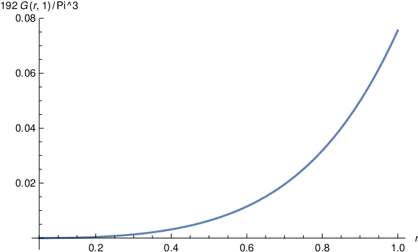
Figure 2: Plot of the function (192/π3)​G​(r,1)(192/\pi^{3})G(r,1).

Combining (14) with (24) and (31), adding the result (10) (for α=+,−\alpha=+,-), the known order kF5​(kF​R)k_{\rm F}^{5}(k_{\rm F}R) contribution C0​pF−2​pF+2/36​π4C_{0}p_{{\rm F}-}^{2}p_{{\rm F}+}^{2}/36\pi^{4}, the contribution of order kF5​(kF​R)2k_{\rm F}^{5}(k_{\rm F}R)^{2}

64​mf​C02(2​π)6​ℏ2​∫0smaxd​s​s2​14​π​∫d3​𝐭​θ​θ​(−Λ+gfin​(t,s)+t2Λ),\displaystyle{64m_{f}C_{0}^{2}\over(2\pi)^{6}\hbar^{2}}\int_{0}^{s_{\rm max}}\!ds~\!s^{2}~\!{1\over 4\pi}\int\!d^{3}\mathbf{t}~\!\theta~\!\theta\left(-\Lambda+g_{\rm fin}(t,s)+{t^{2}\over\Lambda}\right), (32)

obtained in [13] and finally expressing the couplings C0C_{0}, C2C_{2} and C2′C_{2}^{\prime} in terms of the ss and pp-wave scattering lengths a0a_{0}, a1a_{1} and the ss-wave effective radius r0r_{0} using (9) one easily finds (using the results of [13]) that up to the order kF5​(kF​R)3k_{\rm F}^{5}(k_{\rm F}R)^{3} all terms diverging with Λ→∞\Lambda\rightarrow\infty cancel out. One observes that the finite contribution arising in (32) from the term proportional to 1/Λ1/\Lambda after it is multiplied by the term ∝Λ\propto\Lambda present in C02C_{0}^{2} cancels against the finite term −2​t2-2t^{2} arising from squaring the function (17) in the contribution of the “particle-particle” diagram. Such terms must cancel because they would be absent had one used Dimensional Regularization instead of the cutoff Λ\Lambda. Defining then

G⁡(pF−,pF+)=Gfin(1)​(pF−,pF+)+G(2)​(pF−,pF+),\displaystyle G(p_{{\rm F}-},~\!p_{{\rm F}+})=G^{(1)}_{\rm fin}(p_{{\rm F}-},~\!p_{{\rm F}+})+G^{(2)}(p_{{\rm F}-},~\!p_{{\rm F}+})~\!,
K⁡(pF−,pF+)=K(1)​(pF−,pF+)+K(2)​(pF−,pF+),\displaystyle K(p_{{\rm F}-},~\!p_{{\rm F}+})=K^{(1)}(p_{{\rm F}-},~\!p_{{\rm F}+})+K^{(2)}(p_{{\rm F}-},~\!p_{{\rm F}+})~\!, (33)

where Gfin(1)​(pF−,pF+)G^{(1)}_{\rm fin}(p_{{\rm F}-},~\!p_{{\rm F}+}) is given by the formula (15) with g⁡(t,s)g(t,s) replaced by gfin​(t,s)g_{\rm fin}(t,s) one arrives at the final formula

EΩV=16​π2ℏ22​mf{35(pF−5+pF+5)+43​πpF−3pF+3a0+192π2a02J(pF−,pF+)\displaystyle{E_{\Omega}\over V}={1\over 6\pi^{2}}~\!{\hbar^{2}\over 2m_{f}}\left\{{3\over 5}\left(p_{{\rm F}-}^{5}+p_{{\rm F}+}^{5}\right)+{4\over 3\pi}~\!p_{{\rm F}-}^{3}p_{{\rm F}+}^{3}~\!a_{0}+{192\over\pi^{2}}~\!a_{0}^{2}~\!J(p_{{\rm F}-},~\!p_{{\rm F}+})\right.\phantom{aaaaaaaa}~\!
+384π3​a03​G​(pF−,pF+)−96π3​a03​K​(pF−,pF+)\displaystyle+{384\over\pi^{3}}~\!a_{0}^{3}~\!G(p_{{\rm F}-},~\!p_{{\rm F}+})-{96\over\pi^{3}}~\!a_{0}^{3}~K(p_{{\rm F}-},~\!p_{{\rm F}+})\phantom{aaaa}~\!
+110​π​a02​r0​pF−3​pF+3​(pF−2+pF+2)\displaystyle+{1\over 10\pi}~\!a^{2}_{0}r_{0}~\!p^{3}_{{\rm F}-}p^{3}_{{\rm F}+}\left(p_{{\rm F}-}^{2}+p_{{\rm F}+}^{2}\right)\phantom{aaaaaaaaaaaaa}~ (34)
+15​πa13[2pF−8+2pF+8+pF−3pF+3(pF−2+pF+2)]}.\displaystyle\left.+{1\over 5\pi}~\!a_{1}^{3}\left[2p^{8}_{{\rm F}-}+2p^{8}_{{\rm F}+}+p^{3}_{{\rm F}-}p^{3}_{{\rm F}+}\left(p_{{\rm F}-}^{2}+p_{{\rm F}+}^{2}\right)\right]\right\}.

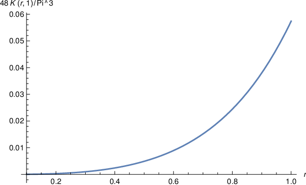
The function J⁡(pF−,pF+)J(p_{{\rm F}-},p_{{\rm F}+}) is defined in [13]. It is also easy too see that J⁡(pF−,pF+)=pF+7​J​(r,1)J(p_{{\rm F}-},~\!p_{{\rm F}+})=p_{{\rm F}+}^{7}J(r,1), G⁡(pF−,pF+)=pF+8​G​(r,1)G(p_{{\rm F}-},~\!p_{{\rm F}+})=p_{{\rm F}+}^{8}G(r,1) and K⁡(pF−,pF+)=pF+8​K​(r,1)K(p_{{\rm F}-},~\!p_{{\rm F}+})=p_{{\rm F}+}^{8}K(r,1). The plot of the function J⁡(r,1)J(r,1) has been given in [13]. The functions (192/π3)​G​(r,1)(192/\pi^{3})G(r,1) and (48/π3)​K​(r,1)(48/\pi^{3})K(r,1) are shown here in Figures 2 and 3, respectively.

Refer to caption
Figure 3: Plot of the function (48/π3)​K​(r,1)(48/\pi^{3})K(r,1).

In the limit pF−=pF+=kFp_{{\rm F}-}=p_{{\rm F}+}=k_{\rm F} the result (34) should coincide with

EΩV=16​π2ℏ22​mf{gs35kF5+gs(gs−1)23​πkF6a0+gs(gs−1)4​(11−2​ln⁡2)35​π2kF7a02\displaystyle{E_{\Omega}\over V}={1\over 6\pi^{2}}~\!{\hbar^{2}\over 2m_{f}}\left\{g_{s}~\!{3\over 5}~\!k_{\rm F}^{5}+g_{s}(g_{s}-1)~\!{2\over 3\pi}~\!k_{\rm F}^{6}a_{0}+g_{s}(g_{s}-1)~\!{4(11-2\ln 2)\over 35\pi^{2}}~\!k_{\rm F}^{7}a_{0}^{2}\right.\phantom{aaaaa}
+[gs​(gs−1)​N1+gs​(gs−1)​(gs−3)​N2]​kF8​a03\displaystyle+[g_{s}(g_{s}-1)~\!N_{1}+g_{s}(g_{s}-1)(g_{s}-3)~\!N_{2}]~\!k_{\rm F}^{8}~\!a_{0}^{3}\phantom{aaaaaaaaaaa}
+gs(gs−1)110​πkF8a02r0+gs(gs+1)15​πkF8a13},\displaystyle\left.+g_{s}(g_{s}-1)~\!{1\over 10\pi}~\!k^{8}_{\rm F}~\!a_{0}^{2}r_{0}+g_{s}(g_{s}+1)~\!{1\over 5\pi}~\!k^{8}_{\rm F}~\!a_{1}^{3}\right\},\phantom{aaaaaaaa}~ (35)

for gs=2g_{s}=2 given in [7] and [12] with N1=0.07550±0.00003N_{1}=0.07550\pm 0.00003 and N2=0.05741±0.00002N_{2}=0.05741\pm 0.00002 in [7], and N1=0.0755732N_{1}=0.0755732 and N2=0.0573879N_{2}=0.0573879 in [12]. Numerical evaluation of the functions (192/π3)​G​(1,1)(192/\pi^{3})G(1,1) and (48/π3)​K​(1,1)(48/\pi^{3})K(1,1) - the endpoints in Figures 2 and 3, respectively - gives N1=0.0755617N_{1}=0.0755617 and N2=0.057387N_{2}=0.057387 in good agreement with the numbers obtained in [7] and [12]. (In [13] it has been found that J⁡(1,1)=0.0114449J(1,1)=0.0114449 which with high accuracy equals (11−2​ln⁡2)/840(11-2\ln 2)/840).

Expressed in terms of kF=(3​π2​N/V)1/3k_{\rm F}=(3\pi^{2}N/V)^{1/3} and rr the formula (34) takes the form

EΩV=kF33​π2ℏ2​kF22​mf35{12(1+r5)(21+r3)5/3+109​πr3(21+r3)2(kFa0)\displaystyle{E_{\Omega}\over V}={k_{\rm F}^{3}\over 3\pi^{2}}~\!{\hbar^{2}k_{\rm F}^{2}\over 2m_{f}}~\!{3\over 5}\left\{{1\over 2}\left(1+r^{5}\right)\!\left({2\over 1+r^{3}}\right)^{5/3}+{10\over 9\pi}~\!r^{3}\!\left({2\over 1+r^{3}}\right)^{2}\left(k_{\rm F}a_{0}\right)\right.\phantom{aaaaaaaaaaaaaaaaaa}
+160π2​(21+r3)7/3​J​(r,1)​(kF​a0)2\displaystyle+{160\over\pi^{2}}\left({2\over 1+r^{3}}\right)^{7/3}\!J(r,1)\left(k_{\rm F}a_{0}\right)^{2}\phantom{aaaaaaaaaaaaaaaaaaaaaaaaaaaaaaaa} (36)
+80π3​(21+r3)8/3​[4​G​(r,1)−K⁡(r,1)]​(kF​a0)3\displaystyle+{80\over\pi^{3}}\left({2\over 1+r^{3}}\right)^{8/3}\!\left[4~\!G(r,1)-K(r,1)\right]\left(k_{\rm F}a_{0}\right)^{3}\phantom{aaaaaaaaaaaaaaaaaaaaaa}
+112​π(21+r3)8/3[r3(1+r2)(kF3a02r0)+2(2+2r8+r3+r5)(kFa1)3]}.\displaystyle\left.+{1\over 12\pi}\left({2\over 1+r^{3}}\right)^{8/3}\!\!\left[r^{3}(1+r^{2})~\!(k^{3}_{\rm F}a_{0}^{2}r_{0})+2(2+2r^{8}+r^{3}+r^{5})(k_{\rm F}a_{1})^{3}\right]\right\}.

The third order corrections computed in this work (the last two lines in the above formula) are rather small. For r0=a1=0r_{0}=a_{1}=0 (i.e. without the contribution on the dimension R−6R^{-6} operators) the ratio of the order (kF​a0)3(k_{\rm F}a_{0})^{3} contribution to the first term in the curly brackets increases from 0.00003 at kF​a0=0.1k_{\rm F}a_{0}=0.1 to 0.030.03 at kF​a0=1k_{\rm F}a_{0}=1. This can be compared to the analogous ratio of the order (kF​a0)2(k_{\rm F}a_{0})^{2} term which at r=1r=1 increases from 0.00185 to 0.185. These ratios decrease further with decreasing rr (increasing polarization) and become exactly zero at r=0r=0 due to the Pauli exclusion which forbids any contribution to the ground state energy to be generated by the interaction operator proportional to C0C_{0}.

Refer to caption
Figure 4: Energy density EΩ/VE_{\Omega}/V in units (3/5)​ℏ2​kF5/6​π2​mf=(N/V)​(ℏ2​kF2/2​mf)​(3/5)(3/5)\hbar^{2}k^{5}_{\rm F}/6\pi^{2}m_{f}=(N/V)(\hbar^{2}k^{2}_{\rm F}/2m_{f})(3/5) of the gas of spin 1/21/2 fermions as a function of its polarization P=(N+−N−)/NP=(N_{+}-N_{-})/N for different values (from below) 0.2 (blue), 0.4 (yellow), 0.6 (green) of the expansion parameter kF​a0k_{\rm F}a_{0}. The last curve (red) corresponding to kF​a0=0.6k_{\rm F}a_{0}=0.6 shows the same quantity but without the order (kF​a0)3(k_{\rm F}a_{0})^{3} correction.

The plot of the system’s ground state energy density as a function of the polarization PP related to rr by r⁡(P)=((1−P)/(1+P))1/3r(P)=((1-P)/(1+P))^{1/3} is shown in Fig. 4 for three different values of the expansion parameter kF​a0k_{\rm F}a_{0} (keeping r0=a1=0r_{0}=a_{1}=0). All curves merge at P=1P=1 as a result of the Pauli exclusion principle. The curve corresponding to kF​a0=0.6k_{\rm F}a_{0}=0.6 can be directly compared to the lowest curve shown in Fig. 3 of ref. [4] which shows a numerical estimate of the exact ground state energy obtained using the Quantum Monte Carlo method for a specific model repulsive potential. Consistently with the comparison of the ground state energies of the unpolarized system (P=0P=0 or r=1r=1) made in Fig. 2 of ref. [4], our green curve (for kF​a0=0.6k_{\rm F}a_{0}=0.6) is systematically below its counterpart in Fig. 3 of ref. [4] but the comparison with the red curve of Figure 4 shows that the third order correction computed in this work has the tendency to reduce the difference between the perturbative and Monte Carlo estimates. In general, the comparison with the results of ref. [4] show that the perturbative expansion is reliable up to kF​a0∼<0.5k_{\rm F}a_{0}\stackrel{{\scriptstyle<}}{{{}_{\sim}}}0.5.

Summary. In this work we have reproduced the third order formula for the ground-state energy of the unpolarized gas of spin ss fermions and extended it to the case of the arbitrarily polarized gas of spin 1/21/2 fermions. We have checked the cancellation of all ultraviolet divergences occurring when the result is expressed in terms of the ss-wave scattering length a0a_{0} and worked out analytically the most important integrals occurring in the computation of the relevant Feynman (Hughenholtz) diagrams. This allowed to compute the remaining integrals numerically using the standard Mathematica built-in routines; the resulting final third order formula for the ground state energy of the arbitrarily polarized gas of spin 1/21/2 fermions is given in terms of two new functions of the system’s polarization for which the convenient interpolating formula can be easily obtained. The numerical results suggest that for kF​R∼<0.5k_{\rm F}R\stackrel{{\scriptstyle<}}{{{}_{\sim}}}0.5 the perturbation series for the ground-state energy is well convergent but is not reliable for higher values of the expansion parameter for which the system is expected to exhibit the phase transition to the ordered phase. One may hope, however, that supplemented with a reliable extrapolation procedure the perturbative series will be able to give valuable information about the nature of the phase transition. Further extension of our work to the case of arbitrary mixture of different spin projections of spin ss fermions (in the spirit of [15]) is straightforward.

References

  • [1] K. Huang, Statistical Mechanics, John Willey and Sons, Inc., New York 1963.
  • [2] A.L. Fetter and J.D. Walecka, Quantum Theory of Many Particle Systems, McGraw Hill, 1971.
  • [3] see e.g. L.P. Pitaevskii, Rev. Mod. Phys. 80 1215, (2008); C. Chin, R. Grimm, P. Julienne and E. Tiesinga, Rev. Mod. Phys. 82 1225, 2010,
  • [4] S. Pilati, G. Bertaina, S. Giorgini and M. Troyer, Phys. Rev. Lett. 105, 030405 (2010), arXiv:1004/1169 [cond-mat.quant-gas].
  • [5] E. Fratini, S. Pilati, Phys. Rev. A90, 023605 (2012).
  • [6] S. Pilati, I. Zintchenko and M. Troyer, Phys. Rev. Lett. 112, 015301 (2014), arXiv:1308/1672 [cond-mat.quant-gas].
  • [7] H.-W. Hammer, R. J. Furnstahl, Nucl. Phys. A678, 277 (2000); arXiv:0004043 [nucl-th].
  • [8] R.J. Furnstahl, H.-W. Hammer and N. Tirfessa, Nucl. Phys. A689, 846 (2001).
  • [9] R.J. Furnstahl and H.-W. Hammer, Phys. Lett. B531, 203 (2002).
  • [10] H.-W. Hammer, S. König and U. van Kolck, Rev. of Mod. Phys. 92 (2020), 025004.
  • [11] see e.g. Proceedings of the Joint Caltech/INT Workshop Nuclear Physics with Effective Field Theory, ed. R. Seki, U. van Kolck and M. Savage (World Scientific, 1998); Proceedings of the INT Workshop Nuclear Physics with Effective Field Theory II, ed. P.F. Bedaque, M. Savage, R. Seki and U. van Kolck (World Scientific, 2000).
  • [12] C. Wellenhofer, C. Drischler and A. Schwenk, Phys. Lett. B 802 135247 (2020) arXiv:1812.08444 [nucl-th]; Phys. Rev. C104, 014003 (2021) arXiv:2102.05966 [cond-mat.quant-gas].
  • [13] P.H. Chankowski and J. Wojtkiewicz, Phys. Rev. B104.144425 (2021) arXiv:2108.00793 [cond-mat.quant-gas].
  • [14] S. Kanno, Prog. Theor. Phys. 44, 813 (1970).
  • [15] J. Pera, J. Casulleras and J. Boronat, arXiv:2205.13837 [cond-mat.quant-gas].
  • [16] E. Stoner, The London, Edinburgh and Dublin Phil. Mag. and Journal of Science 15 (1933), 1018.
  • [17] R.J. Furnstahl, V. Steele and N. Tirfessa, Nucl. Phys. A671 (2000), 396.
  • [18] W. Lenz, Z. Phys. 56, 778 (1929).
  • [19] S. Weinberg, The Quantum Theory of Fields, Vol. I, The Press Syndicate of the University of Cambridge, 1995.
  • [20] K. Huang and C.N. Yang, Phys. Rev. 105, 767 (1957), T.D. Lee and C.N. Yang, Phys. Rev. 105, 1119 (1957).
  • [21] P.H. Chankowski and J. Wojtkiewicz, in preparation.