Provably efficient variational generative modeling of quantum many-body systems
via quantum-probabilistic information geometry
Abstract
The dual tasks of quantum Hamiltonian learning and quantum Gibbs sampling are relevant to many important problems in physics and chemistry. In the low temperature regime, algorithms for these tasks often suffer from intractabilities, for example from poor sample- or time-complexity. With the aim of addressing such intractabilities, we introduce a generalization of quantum natural gradient descent to parameterized mixed states, as well as provide a robust first-order approximating algorithm, Quantum-Probabilistic Mirror Descent. We prove data sample efficiency for the dual tasks using tools from information geometry and quantum metrology, thus generalizing the seminal result of classical Fisher efficiency to a variational quantum algorithm for the first time. Our approaches extend previously sample-efficient techniques to allow for flexibility in model choice, including to spectrally-decomposed models like Quantum Hamiltonian-Based Models, which may circumvent intractable time complexities. Our first-order algorithm is derived using a novel quantum generalization of the classical mirror descent duality. Both results require a special choice of metric, namely, the Bogoliubov-Kubo-Mori metric. To test our proposed algorithms numerically, we compare their performance to existing baselines on the task of quantum Gibbs sampling for the transverse field Ising model. Finally, we propose an initialization strategy leveraging geometric locality for the modelling of sequences of states such as those arising from quantum-stochastic processes. We demonstrate its effectiveness empirically for both real and imaginary time evolution while defining a broader class of potential applications.
I Introduction


Quantum machine learning can be bifurcated as two principal research directions depending on the nature of the data specification anshu2022some; broughton2020tensorflow. On one hand, the learning problem may be specified in terms of classical data and so have associated classical algorithmic baselines. The prospect of quantum advantage (when a quantum computer enables an exponential speedup over a classical baseline wang2022quantum) has sparked significant research efforts on quantum algorithms for classical data. For example, sparse matrix inversion is BQP-complete and so expected to admit such an advantage harrow2009quantum. However, a broader class of once anticipated advantages was shown to be an artifact of state preparation assumptions rather than following from the quantumness of the algorithms tang2021quantum; tang2019quantum. In particular, many speedups vanish if one has classical -sampling access to the same data (which is at least as easy to obtain as quantum state preparation). Several additional theoretical mcclean2018barren; wang2021noise and practical giovannetti2008quantum; aaronson2015read; broughton2020tensorflow barriers have emerged along this direction, though key milestones in understanding have been reached liu2021rigorous; arunachalam2017guest; arunachalam2022quantum.
On the other hand, separate, exciting efforts are analyzing the problem of efficiently learning (or simulating) properties of unknown (or, respectively, known) quantum systems aaronson2019shadow; huang2020predicting; huang2021quantum; huang2021information; huang2021provably; arute2019quantum which serve as quantum data. Hence, all relevant algorithms are quantum since, at the least, they require measuring (or preparing) a quantum system. For learning, the required data samples can scale as poorly as exponentially in the number of qubits vogel1989determination. Dealing with the quantum nature of the data in order to tame such scalings does not necessarily require entirely foreign algorithmic ideas compared to the classical; in many cases (e.g., brandao2019quantum; szegedy2004quantum; yung2012quantum; anshu2021sample; haah2021optimal; liu2019quantum), so-called “quantization” of classical techniques describes the fruitful methodology of (sometimes systematically) adjusting these techniques to integrate such structure. We will quantize several techniques and proofs in this way.
In this work, we propose a variational approach to a problem which has garnered significant attention, both theoretically swingle2014reconstructing; bairey2019learning; qi2019determining; evans2019scalable; anshu2021sample; haah2021optimal; anshu2022some and experimentally wang2017experimental; senko2014coherent: learning spatially local quantum many-body Hamiltonians. In particular, such an algorithm should ideally be both time-efficient and sample-efficient, and apply to both low- and high-temperature Gibbs states. The low-temperature learning problem arises in a variety of physics kokail2021entanglement; dalmonte2022entanglement and quantum technology settings, for example in relevance to distinguishing quantum phases regnault2017entanglement; haag2012local or holographic entanglement entropy casini2011towards. The classical analogue of this task, learning undirected graphical models or Markov random fields, is central to the machine learning and statistical inference communities chow1968approximating; hinton1986learning; karger2001learning; abbeel2006learning; santhanam2012information; bresler2008reconstruction; bresler2015efficiently; vuffray2016interaction; klivans2017learning.
While few formal results exist, recent trailblazing approaches have yielded provable data sample-efficiency anshu2021sample; haah2021optimal. However, because their proofs assume a particular model11 1 Anshu et al. anshu2021sample and Haah et al. haah2021optimal implicitly assume the Quantum Exponential Family (QEF) yapage2008information. For more details see Section IV.3.1., their methods require classically estimating gradients of the quantum log partition function. This computation is known to suffer from the sign problem henelius2000sign; eisert2020Science, and is generically time-inefficient in the low-temperature regime harrow2020classical. Our proposed algorithm allows us to translate the estimation of a quantum log partition function gradient to a classical one by allowing measurements to be variational. Hence, as we will elaborate, broad classes of Hamiltonians (for example, satisfying the Eigenstate Thermalization Hypothesis deutsch1991quantum; srednicki1994chaos) may be amenable to our approach and not the aforementioned approaches. Our analysis proceeds by showing that our variational algorithm achieves an optimal parameter estimation limit, under certain assumptions, independent of the problem instance or model parameterization. No previous variational quantum algorithm (metric-aware or otherwise) is known to satisfy this criterion.
Furthermore, our result also applies to the historically important feynman1982simulating; lloyd1996universal and presently popular arute2019quantum reverse problem of simulation of quantum states on quantum computers. In particular, we present a sample-efficient variational algorithm for quantum Gibbs sampling of states corresponding to a given Hamiltonian. Quantum Gibbs sampling is important because it enables the study of non-zero-temperature physics on quantum computers kassal2011simulating; motta2019qite; dallaire2016method; cohn2020minimal; sun2021qite; bauer2020quantum. It is also an important subroutine for a range of quantum algorithms seeking quantum advantage brandao2017quantum; van2019improvements; brandao2019quantum; van2020quantum; brandao2022faster; montanaro2015quantum; harrow2020adaptive; lloyd2014quantum. Our data-sample-efficiency result is the first such concrete statement for variational quantum Gibbs sampling, and carries the same model choice flexibility.
For both scenarios of learning and simulation, we observe numerical advantage over existing optimizers. In particular, such advantages are facilitated by a novel technique which translates the analogous second-order algorithm to a robust, first-order approximation. This is a quantization of a classical result raskutti2015information. Finally, we will see empirically, and motivate in connection with our sample-efficiency result, that our approach is particularly conducive to learning or simulating sequences of quantum states. This problem arises in a variety of contexts including molecular geometry optimization nagaoka2003structure, annealing apolloni1989quantum; apolloni1990numerical; finnila1994quantum, and time evolution abrams1997simulation; kassal2008polynomial; mcardle2020quantum.
II Overview of contributions
II.1 Efficient learning and sampling of many-body states
An important learning for quantum data problem is the quantum Hamiltonian learning problem, which has recently received much attention in the quantum community wiebe2014quantum; wiebe2014bhamiltonian; wang2017experimental; bairey2019learning; qi2019determining; evans2019scalable; bairey2020learning; anshu2021sample; haah2021optimal; anshu2022some. The goal is to learn the Hamiltonian of a quantum many-body system from copies of its Gibbs state, which describes the equilibrium state of a system that is in contact with a heat bath.
More technically, consider a quantum system of qubits and a -local modular Hamiltonian having coefficients over a finite-dimensional lattice, and are known non-identity Pauli operators. Furthermore, the interaction graph is assumed to be spatially local so that in terms of the number of qubits. Then, given copies of the Gibbs state :
| (1) |
where is inverse to temperature, the goal is to learn the coefficients to additive error , or equivalently, to learn the vector to error in -norm.
Recently, Anshu, Arunachalam, Kuwahara, and Soleimanifar anshu2021sample studied the sample complexity of a simple approach which involves measuring in the basis and then solving a classical optimization problem (the so-called maximum entropy problem). They found that this approach is learned to error with probability at least using
| (2) |
data samples haah2021optimal, where are geometric constants22 2 The existence of the factor exponential in can be attributed to the fact that finding ground states of local Hamiltonians is QMA-complete kempe2006complexity.. Hence, this approach is sample-efficient in number of qubits and, in fact, best-known for general . On the other hand, the algorithm implicitly assumes a particular model, the quantum exponential family33 3 Also known as a quantum Boltzmann machine yapage2008information; amin2018quantum. See Sections IV.3.1 and F.2.. This assumption requires their algorithm to compute gradients of a quantum log partition function. For low temperatures, this computation can become QMA-hard wei2009interacting; aharonov2009power; harrow2020classical; alhambra2022quantum, causing classical simulation to become intractable temme2011quantum; yung2012quantum; tan2022sign.
In our work, we design and analyze a variational approach to quantum Hamiltonian learning. It is a quantum variety of online natural gradient descent with a special choice of metric over the quantum mixed state manifold. Because it generalizes quantum natural gradient descent to quantum mixed states, we call it QPNGD 44 4 The word “probabilistic” is used to distinguish our algorithm from the pure state version described in existing literature, displayed as Algorithm 1. It solves the same task using the polynomial scaling of Anshu et al. (2)55 5 For sufficiently small , and assuming asymptotic convergence; see Section D.5., while enabling flexibility in the choice of model (as we will elaborate). One motivated choice is a diagonal ansatz which fits the spectral decomposition of the target state verdon2019qhbm; this choice turns the quantum log partition function into a classical one, so that roadblocks like the sign problem eisert2020Science encountered when attempting to sample from a quantum exponential family model can be circumvented66 6 See e.g. alhambra2022quantum for a pedagogical review of the complexity of thermal states..
As a motivating example, under the Eigenstate Thermalization Hypothesis (ETH) assumption deutsch1991quantum; srednicki1994chaos, the quantum Metropolis sampling algorithm temme2011quantum has been shown to converge efficiently which is unexpected for classical methods chen2021fast. Quantum Metropolis sampling similarly diagonalizes the density operator in question so that the sampling becomes classical, but does so via the fault-tolerant quantum phase estimation algorithm. Hence, for our variational approach to be successful, a suitable fixed-depth diagonal ansatz must be posited, the difficulty of which is subject to recent, promising discussion larose2019variational; cerezo2020variational. Furthermore, as we will discuss in Section IV.3.1, this flexibility may allow one to relax the prior information required to specify a sample-efficient model for certain problem instances.
To obtain the sample efficiency result, we consider the idea of Fisher efficiency, and describe its quantum analogue quantum Fisher efficiency. These broadly applicable optimality properties would be a desirable feature of any variational update rule. Quantum and classical Fisher efficiency take the perspective of viewing descent rules as parameter estimation (metrological) strategies, and so we offer a bridge between the mature field of quantum metrology and the contemporary field of quantum variational optimization. As we will demonstrate, our particular metric-aware descent rule, under a specific choice of metric, is first-known to satisfy this criterion in quantum stokes2020quantum; koczor2019quantum; van2020measurement (Theorem IV.1).
II.2 Optimization robustness via convex duality
There are important practical considerations required to achieve the efficient scaling and manageable constant factors in Equation 2. Perhaps most notably, Algorithm 1 requires estimating and inverting a second-order metric quantity, a task which requires collecting quadratic-scaling samples77 7 See Section V for the calculation. from one’s model at each optimization step.
In the classical literature, a result is known which translates our second-order optimization problem to a dual first-order one called mirror descent raskutti2015information. As we will find, a special choice of metric over the quantum mixed state manifold – the same choice which enables our efficiency result (2) — allows us to derive a novel quantized version of this mirroring duality. This duality is stated in Theorem V.1. We leverage this result into a novel quantum optimization algorithm, QPMD, displayed as Algorithm 2. We find numerically (see Footnotes 33 and 5) that this algorithm is more robust than QPNGD during optimization.
To understand the utility of going to first order, it is useful to note the distinction between data and model sample complexities. For learning, this depends on whether a sample is drawn by re-preparing the ground truth (data) thermal state or the model thermal state88 8 This is in tune with the classical distinction made implicitly by Amari amari1998natural in that one data sample is used at each optimizaton step for online natural gradient descent whereas, e.g., the information matrix (which depends only on the probabilistic model) is estimated without error.. The efficient scaling (2) concerns the number of data thermal state re-preparations, also called data sample complexity, which may be the key resource of interest. On the other hand, there is an assumption that the metric quantity, which requires no data samples, is estimated sufficiently accurately. This may be costly in terms of the number of model state re-preparations required. Similarly, for simulation, the data sample complexity concerns only the number of measurements of the input Hamiltonian on the prepared state.
Existing algorithms, both quantum stokes2020quantum and classical martens2015optimizing; raskutti2015information, which require estimating and inverting a metric quantity have recognized that taming the model sample scaling is critical for practical applications. In quantum, block approximations stokes2020quantum have been considered as mechanisms to limit the computation of cross terms to pairs of parameters which are expected to be significantly correlated. Related types of inductive biases have been successful classically, for example assuming that the information matrix has a Kronecker product factorization martens2015optimizing.
The exact or approximate duality implies a potentially more robust update rule which exactly or approximately recovers the data samples scaling (2). As we have noted, the improved model sample-efficiency is due to each iteration of the mirror descent update rule requiring solving a sub-problem which is first-order. This sub-problem requires computing gradients in the quantum relative entropy, a task to which the Quantum Hamiltonian-Based Model (QHBM) ansatz99 9 See Appendix G for a self-contained review. of a Gibbs state is particularly amenable verdon2019qhbm and is non-trivial for general ansatze amin2018quantum, as we will discuss1010 10 See Section IV.3.1..
II.3 Efficient learning and Gibbs sampling of sequences of states
In proving the quantum Fisher efficiency result, the neighborhood of “fast convergence” occurs when the third-order terms in the Taylor expansion of the loss go to zero sufficiently quickly (Section VII.3). Intuitively, this describes the regime for which the optimization problem is approximately convex quadratic. In many important applications, the fineness of the path discretization is a control parameter and so we provide a criterion in Equation 18 by which one could choose a discretization where the optimality still holds (Section VII.3).
We can use this intuition to motivate one class of problems where these guarantees may then more consistently apply: the learning and Gibbs sampling of sequences of quantum states. As we will discuss, this type of problem shows up in many contexts including molecular geometry optimization nagaoka2003structure, quantum annealing apolloni1989quantum; apolloni1990numerical; finnila1994quantum, and time evolution abrams1997simulation; kassal2008polynomial; mcardle2020quantum. In these scenarios, after learning the first state in a sequence of sufficiently close1111 11 In the sense of quantum-statistical distance, quantified via the metric as in Section III.2 density operators, initializing one’s learning at the previous optimum in the sequence may make optimization approximately convex quadratic. We discuss sequence learning in detail in Section VII, and observe that this straightforward initialization strategy leads to promising performance improvements.
III Background
III.1 Loss functions for density operators
Work in Variational Quantum Algorithms (VQAs) mcclean2016theory; preskill2018quantum; cerezo2021variational has shown that it can be advantageous to allow the resources used for a quantum task to be tunable. For such algorithms, a fixed depth circuit is re-run as its parameters are tuned, rather than appending additional fixed circuits at each step of the algorithm. Lending theoretical justification to this strategy is the result that physical states make up an exponentially small submanifold of Hilbert space poulin2011quantum, so that correspondingly, a quantum circuit ansatz may need only a small number of parameters to learn quantum states of interest.
To formalize these ideas, let be the set of density operators1212 12 Equivalently, density matrices or quantum mixed states. We note that our notation in this section follows conventions in bengtsson2017geometry . Suppose we want to learn some unknown quantum state represented by density operator . We take the strategy of positing a parametric model murphy2012machine with parameters . The parameters are to be tuned until . Note that both quantum Hamiltonian learning and quantum Gibbs sampling can be phrased in terms of learning a parametric model for a target density operator verdon2019qhbm.
To measure how well our parameterized model approximates , we need to define a loss function. Generally speaking, a loss function is a map which uses information about the target data set to map a parameterized model to the real numbers, . In this paper we will let our loss functions be defined in terms of functions acting on pairs of density operators,
| (3) |
We require to be a contrast functional. We say that is a constrast functional1313 13 Our use of the term contrast functional is consistent with petz2002covariance; jencova2004generalized. Those are quantum generalizations of the related term “contrast function” used in the classical literature pfanzagl1973asymptotic; eguchi1983second if it is a non-negative smooth function petz2002covariance such that
| (4) |
This property allows us to identify when we have perfectly learned the target state. In the next section we describe how it allows us to relate metrics for quantum information geometry to loss functions on our parametric models.
Now we have all the components necessary to phrase state learning as a parameter optimization problem. Given our parametric model , target data density operator , and our choice of loss function , state learning is simply the task of finding . In other words, we find the minimum of the loss function.
In VQAs, it can be advantageous to leverage gradient information to perform the minimization of the loss harrow2021lowdepth. In the next section we discuss formal structures, Riemannian manifolds of density operators, which will help us best leverage gradient information to optimize the loss.
III.2 Riemannian manifolds of density operators
The algorithms we will introduce in later sections depend on the mathematical concept of a Riemannian manifold. In this subsection, we review some known results at the intersection of manifolds and density operators that we intend to leverage1414 14 See Appendix B for further discussion..
Manifolds generalize calculus to sets of objects beyond vectors of real numbers frankel2012geometry. Speaking loosely, a manifold is a continuous set of objects labelled by smooth coordinate functions which map one-to-one with Euclidean space. In our setting, the objects are given by the set of density operators, . The parametric model which we have posited has a so-called hypothesis class which spans some subset of . Informally, we can think about the parameters of this model as serving as the smooth coordinates. Formally, however, the one-to-one property is not anticipated to be met in general, particularly when certain inductive architectural biases are leveraged or the model specification includes a neural network1515 15 Nevertheless, it is possible to choose a model parameterization so as to describe a smooth embedding from classical (Euclidean) parameter space to (Section G.2).. This observation has noteworthy implications that we will discuss; for example, introducing a pseudo-inverse and breaking down exact invariance under re-parameterization for metric-aware descent (Algorithm 1).
Given some new parameters near , we again need a quantitative way to distinguish the updated model from . The mathematical tool for doing so on a manifold is the metric which defines an inner product taking arguments in the tangent space about . Adding a metric to our manifold of models turns it into a Riemannian manifold.

A standard property to require of a metric over a statistical manifold is monotonicity. Recall that every physical process in quantum mechanics can be represented by a Completely-Positive Trace Preserving (CPTP) map, also called a quantum channel wilde2017quantum. Let and be any two vectors in the tangent space at and let be any quantum channel. Then, a metric is monotone if
| (5) |
is true for all , , and bengtsson2017geometry. Intuitively, a quantum channel may coarse-grain, or randomize, the state on which it acts; monotonicity says such randomization does not help in distinguishing states.
Furthermore, we will find it convenient to resolve the metric tensor to coordinates as a matrix. We will define the Information Matrix as having matrix elements
| (6) |
This matrix is positive definite so long as gives a basis for , the tangent space of at (Corollary B.5.1). Then, we have the result that is the Hessian of some contrast functional (Equation 4) lesniewski1999monotone; jencova2004generalized,
| (7) |
Since our losses are defined in terms of contrast functionals (recall Equation 3), Equation 7 tells us that taking the Hessian of our loss turns it into a valid monotone metric.
In the classical case, density operators are instead categorical probability distributions and in (8) is uniquely the classical relative entropy1616 16 C̆encov’s theorem cencov2000statistical says that, for categorical distributions, the Fisher-Rao metric is the unique metric (up to normalization) which satisfies the analogous monotonicity property. See Section B.1.. In this case, the information matrix is the classical Fisher information matrix. In the quantum case, the option set is broader and so we will find it valuable to consider the choice of metric carefully.
Figure 2 illustrates the main features of our manifold perspective on quantum state learning. It includes the full manifold of density operators, the submanifold spanned by our parametric model, the map between coordinate space and model space , and the information matrix .
III.3 Natural gradient descent
In the previous section, we phrased the task of variational learning and Gibbs sampling as an optimization problem over a Riemannian manifold of parametric models. Evidently, there are many different ways to perform such optimization. For example, we may seek an update rule which travels in a locally optimal fashion over the manifold in the sense of most rapidly reducing the loss. It is understood that natural gradient descent offers such behavior, and we will re-express a well-known characterization amari2016information for completeness. Since such a rule depends only on the search space as opposed to the classically parameterizing space, we diminish liang2019fisher (and, in some cases, eliminate amari1998natural) dependencies on the choice of classical parameterization1717 17 See Section E.3..
In particular, suppose we start at some parameter setpoint with associated loss function value . Optimizing our parametric model means changing the parameters by some update vector to some new value such that we expect . To find the direction of steepest descent, we first use the contrast functional associated to our loss function to fix a local neighborhood on our manifold anchored at . Then, we optimize the direction of restricted to that neighborhood:
| (8) |
where is a small constant. Intuitively, as we can think of (locally) as a distinguishability function over , this objective enforces that we update parameters so as to choose optimally from a ball of equally distinguishable operators relative to the current guess.
Writing the objective (8) as a Lagrangian with Lagrange multiplier and expanding to first non-vanishing order can be shown to give (Section D.1)
| (QPNGD) |
where denotes the Moore-Penrose pseudo-inverse of a matrix . This is Algorithm 1. Such update rules are known as natural gradient or metric-aware descent. We show an example trajectory for this algorithm in Figure 1.
Equation QPNGD aesthetically matches the so-called classical natural gradient update rule amari2016information and existing quantum generalizations stokes2020quantum; koczor2019quantum; van2020measurement. However, in the quantum case, existing works have thus far assumed the choice of corresponding to the so-called Bures-Helstrom (BH) metric. In stokes2020quantum, the authors explored this monotone metric in its relevance to pure state optimization where it becomes unique. For mixed states, existing literature has considered the metric induced by the Quantum Fisher Information (QFI) koczor2019quantum; van2020measurement. Doing so may be motivated by a belief that the optimal parameters correspond to an approximately pure density operator, and so suitable low-rank approximations have been considered koczor2019quantum; van2020measurement. In our generic consideration, such near-purity assumptions are not necessary.
Hence, in the next section, we will motivate a different choice of , corresponding to the so-called Bogoliubov-Kubo-Mori (BKM) metric, and find that it allows for so-called quantum Fisher efficient learning.
IV Efficient learning and sampling of many-body states
In this section, we first describe the use of the BKM metric in the QPNGD update rule (QPNGD). Then we discuss how this update rule, under natural assumptions, meets a desirable asymptotic optimality criteria which characterizes optimization convergence. This is analogous to a known classical result amari1998natural, but first-known for quantum. Finally, we interpret this optimality result in terms of many-body learning and simulation problems.
IV.1 Online quantum natural gradient for a special choice of metric
Following (QPNGD), for learning, consider an online metric-aware update rule with a particular choice of learning rate,
| (9) |
where we define to be an online unbiased estimator obtained by the environment drawing a single pure state from the eigenstates of data density operator (with probability of the corresponding eigenvalue) at each optimization step. We choose such that
| (10) |
with being the canonical quantum relative entropy wilde2017quantum, and
| (11) |
Thus, the metric potential, as in (7), is given by the quantum relative entropy (in either direction since they are equivalent up to third-order c.f. Proposition G.5):
| (12) |
Choosing the quantum relative entropy as our contrast functional leads to the BKM metric bengtsson2017geometry.
Before we proceed, we discuss the experimental feasibility of the proposed algorithm. Roughly speaking, the implementation of (9) requires the ability to estimate first- and second-order derivatives in a relative entropy loss. For a general density operator ansatz, this is achievable but involves potentially intractable averaging over a quantum thermal distribution amin2018quantum. To this end, a particular variational ansatz class – termed QHBMs verdon2019qhbm – admits unbiased estimators for these gradients (Section G.1.1) and Hessians (Appendix H) that circumvent such quantum averaging. This works because QHBMs use the spectral representation of a density operator, and so the eigenvalue distribution is classical. Hence, the challenging problem of estimating gradients in the quantum log-partition function becomes a classical (and therefore sign problem free) problem and can be estimated offline from the quantum device. Particularly for low temperatures, this classical problem is still NP-hard in general harrow2020classical; sly2010computational; sly2012computational, but meaningful separation is expected for broad classes of problem instances alhambra2022quantum (see Section IV.3.1). All in all, as a byproduct of diagonalization, QHBMs decouple learning a mixed state into separable quantum and classical statistical learning problems. We refer the reader to Verdon et al. verdon2019qhbm for a comprehensive description of QHBMs, though we provide an overview in Appendix G for completeness.
IV.2 Fisher efficiency
In the classical case, attaining so-called Fisher efficiency roughly means that the asymptotic accuracy of an estimator, as measured by the error covariance matrix, attains the well-known classical Cramér-Rao bound (CRB) to first-order in the number of data samples utilized. We will follow in the steps of Amari amari1998natural and apply this idea to optimization.
We may think of an online optimization rule as a statistical estimator by saying that the latest parameters at step are the estimator given data samples. Fisher efficiency is met for classical online natural gradient descent and a particular choice of learning rate, assuming that the optimal parameters are eventually reached amari1998natural. This implies that, to first-order, such an update rule can achieve the best-case asymptotic measurement scaling which is usually associated to maximum likelihood estimation.
Correspondingly, the quantum analogue of Fisher efficiency, quantum Fisher efficiency, would attain the generalized Quantum Cramér-Rao bound (QCRB) (Appendix C),
| (QFE) |
to first-order in , where is the number of optimization steps. Again, the term on the left-hand side can be thought of as a generalized error covariance relative to the optimal parameters.
In what follows, when we call something “quantum Fisher efficient”, we mean that it attains the generalized QCRB under the BKM metric. The informal theorem statement which follows says that the learning rule (9) is optimal in the sense of (QFE), and similarly a corollary which says that the swapped loss – the one used for variational Gibbs sampling – meets the same optimality criteria. The formal statements and proofs are given in Theorem D.4.
Theorem IV.1.
Corollary IV.1.1.
The equivalent statement holds when one swaps arguments of the loss, .
Note that no particular coordinates or model structure have been chosen for this result. Since the online estimator achieves quantum Fisher efficiency, one can check that using more data samples at each optimization step can only improve convergence and therefore also achieves quantum Fisher efficiency. Again, the update rule (9) is simply the online (QPNGD) where the contrast functional which gives the BKM metric (12) is taken to match the loss, . The corollary follows because is symmetric to third-order and so induces the same local metric as 1818 18 See Section G.1.2 for details on the quantum relative entropy..
There are two intuitive reasons as to why we are able to do this with our particular descent rule and proof strategy. First, we take advantage of the fact that our variational loss will be given precisely by the contrast functional and so the metric evaluated at the optimum is its curvature at the optimum1919 19 It is important to note that is not the Hessian of the loss in general, since its definition (7) is evaluated at , rather than at distinct parameters . Choosing the information matrix to be the Hessian of the loss would make (QPNGD) reduce to an update rule akin to Newton’s method amari2016information.. Hence, optimization steps respect the fundamental distinguishibility of density operators associated to the loss. The fact that the loss curvature and metric did not identify in this way was remarked during the construction of Stokes et al. stokes2020quantum2020 20 Although, a Hölder-like bound on their discrepancy was shown.. The second idea follows the BKM choice of metric and is technical; our proof strategy uses the fact that the derivative of quantum relative entropy in local coordinates can be seen as a quantum expectation of the metric’s so-called logarithmic derivative2121 21 The interested reader may refer to the discussion surrounding and regarding (92)..
In contrast to classical natural gradient descent, no quantum Fisher efficiency result has been shown for prior constructions of quantum metric-aware descent rules stokes2020quantum; koczor2019quantum; van2020measurement. Theorem IV.1 provides such a guarantee. We leave open the possibility of showing quantum Fisher efficiency for other choices of 2222 22 See the discussion in Section IV.2. through a differing proof strategy. Nevertheless, we will show a tractability advantage (Section V.2) which is specific to our choice in Equation 12.
In this sense, it is interesting to consider whether a similar optimality result can be found (through a differing proof strategy2323 23 As has been mentioned, and referring to (92) for details, our proof strategy uses the fact that the derivative of quantum relative entropy in local coordinates can be seen as a quantum expectation of the metric’s so-called logarithmic derivative.) for a distinct choice of contrast functional2424 24 This has been called a generalized quantum relative entropy lesniewski1999monotone. (7) e.g. the one which induces the BH metric. This would be compelling because, for example, the BH instance of quantum Fisher efficiency (QFE) gives the tightest asymptotic scaling guarantee, at least provably in the single-parameter case (Appendix C). To this end, in Proposition C.3, we show that there exists some parameter estimation strategy which can attain the BH scaling for QHBMs since this is not in general guaranteed for an arbitrary parameterization. We leave open the possibility that, in particular, the BH analogue of (9) achieves this scaling.
As in the classical case, the number of model parameters may in general exceed the dimension of the relevant mixed state manifold. In such a case, the information matrix is clearly guaranteed to be singular2525 25 See Proposition G.7 for a reminder. and so Theorem IV.1 does not directly apply. In fact, convergence faster than (QFE) becomes possible due to over-fitting martens2014new, implying a tradeoff with generalization. Nevertheless, classically and under realistic assumptions, convergence rate improvements akin to Theorem IV.1 that do not come at the expense of generalization have been shown for this case by demonstrating that such over-parameterized models behave like their local linear approximations2626 26 This is the well-known Neural Tangent Kernel jacot2018neural idea. Note that the neural network function behaves linearly, but not (in general) the loss. (at the initial parameters) throughout optimization zhang2019fast; cai2019gram; martens2014new. We expect similar guarantees here.
Note as well that, as in the classical analogue, it is assumed that the model parameters eventually converge to the optimal ones. This will not hold in general for non-convex objectives, as are expected with Energy-Based Models (EBMs) and Quantum Neural Networks (QNNs). However, in practice, a reasonable local optimum might be a sufficient proxy for the global optimum, in which case a property analogous to quantum Fisher efficiency may still (approximately) hold martens2014new.
IV.3 Applications
IV.3.1 Sample-efficient learning of many-body states
We now briefly discuss one concrete application of the prescribed update rule being quantum Fisher efficient. As described, for the quantum Hamiltonian learning problem2727 27 In the language of QHBMs, this is the usual type of problem considered when optimizing the reverse relative entropy loss verdon2019qhbm. (Section II.1), it was shown in Anshu et al. that a non-trivial data sample complexity (2), which is polynomial in the number of qudits, can be achieved for general quantum many-body Hamiltonians that are known to have a spatially local interaction graph anshu2021sample. This result analyzes an offline classical learning algorithm known as maximum entropy estimation paired with an assumption that, for qubits, one measures Pauli tensor operators with the appropriate locality.
A key component of the analysis was showing a strong convexity property in the log-partition function. Incidentally, the Hessian of the log-partition function is precisely the BKM information matrix for a particular choice of coordinates, although this connection was not identified by them. Using this strong convexity, we work out in Section D.5 that, for a particular ansatz, quantum Fisher efficiency implies recovering the polynomial sample-efficiency (2). Our result is worked out in Theorem D.8, and of course subject to the same concessions as the quantum Fisher efficiency result itself. Note that the assumption of eventual convergence generally holds for this scenario since it is strongly convex.
The ansatz plugged into quantum Fisher efficiency to achieve this result corresponds to performing the same local, Pauli tensor measurements. In particular, the ansatz is that of a quantum exponential family2828 28 See Section F.1. with a strong inductive bias in that it is assumed that the relevant non-identity Pauli operators are known (an assumption shared with Anshu et al.):
| (13) |
using the notation of Section II.1. The online gradients are worked out in Section F.2.
Existing variational approaches to learning Hamiltonians from Gibbs states have thus far not shown similar, concrete sample-efficiency guarantees yapage2008information; kieferova2017tomography; amin2018quantum; verdon2019qhbm; zoufal2021variational; kokail2021quantum; larose2019variational; cerezo2020variational. Note that we use the same amount of enhancement as the fixed-measurement approaches2929 29 In other words, we do not perform joint measurement over several Gibbs state copies i.e. quantum enhancement huang2021quantum. In fact, for learning, the ansatz which we analyze measures the same observables (Section IV.3.1)..
To understand the impact of this result, we first observe that strong convexity in the loss function applied to the ansatz (13) generally implies expected fast convergence even for vanilla gradient descent. However, we will see from (QPRGF) that when we use the update rule (9) then the same guarantee holds approximately under any smooth, invertible re-parameterization. The ability to re-parameterize, i.e., choose a different model which parameterizes the same subset of spanned by (13), unlocks new routes to tackling time-inefficiency. For example, we will be able to consider models with friendlier gradients that can be more tractably estimated classically. For example, for QHBMs 3030 30 Note that QHBMs can be projected into proper coordinates via the method described in Section G.2., the fact that the model Gibbs state is always represented diagonally allows one to circumvent the log-partition function depending on quantum parameters; instead, the log-partition function depends only on classical parameters. Quantum algorithms which diagonalize density operators so as to translate the sampling problem to be classical are expected to be efficient in broad cases where directly classically sampling from the quantum thermal distribution is not alhambra2022quantum (for example, under the ETH assumption chen2021fast). Given that these quantum algorithms are non-variational, a natural follow-up is to characterize problem-specific time-complexity speedups that may be feasible by means of particular fixed-depth diagonal ansatze.
Even with precise knowledge of the specific relevant instance of (13), positing a distinct model which is an exact re-parameterization may be unrealistic in some cases. However, we may expect similar behavior given a sufficient approximation. In this way, when we do not have the strong prior of knowing the relevant , we may still be able to posit a reasonably approximate re-parameterization of the space spanned by (13). We note that for high temperature (above the phase transition point) a separate approach has been analyzed which delivers optimal sample- and time-complexity with sample complexity and time-complexity haah2021optimal.
IV.3.2 Sample-efficient modelling of Gibbs states
A similar story can be told for the quantum Gibbs sampling literature. In this case, we are given the Hamiltonian as input and may seek to model its corresponding Gibbs state in as few iterations as possible (essentially variational inference murphy2012machine). Similar to the learning problem, at each iteration of variational optimization, we measure the closeness of the model state to the input Hamiltonian by re-preparing the latest model state at least once. For this reverse problem, we recover the same count of required measurements of the known Hamiltonian against the candidate Gibbs state (2). For more discussion on quantum Gibbs sampling, see Section VI. As with learning, a similar polynomial efficiency is expected for variational quantum Gibbs sampling combined with vanilla stochastic gradient descent, if we use the ansatz (13) given the strong convexity chowdhury2020variational. However, again, our method allows flexibility in the choice of model.
V Quantum-Probabilistic Mirror Descent
V.1 Motivation
In Section II.2, we discussed the distinction between model and data samples. We noted in analyzing our online natural gradient update rule that there is an assumption that the metric quantity, which requires no data samples but quadratic-scaling model samples, is estimated sufficiently accurately. This matches the seminal analysis of Amari amari1998natural. In practice, while data state re-preparation may be more costly than model state re-preparation, both are likely to be considered finite resources. Hence, variance in estimation of the information matrix can lead to noisy and ineffective optimization behavior. To address this issue, we derive a robust mirror descent algorithm raskutti2015information (Algorithm 2) which approximates the optimization behavior of metric-aware updates (for a particular choice of metric) without computing any second-order terms directly. Establishing this duality is a first for quantum metric-aware algorithms. Our numerics will corroborate its performance impact (Footnotes 33 and 5).
To see the model sample complexity more explicitly, assume the QHBM ansatz and that the unitary component is parameterized so as to be differentiable through parameter shifts. Recall that, in general, each parameter shift is measured as a separate observable and so the sample cost of parameter shifts will scale as for some small given a desired (in-)accuracy knill2007optimal. Then, estimating the information matrix (7), which has elements, costs parameter shifts where and gives the number of quantum parameters. We work out the estimation of the BKM metric tensor for QHBMs in Appendix H. On the other hand, we can perform each mirror descent update with parameter-shifts where is the number of inner-loop steps in Algorithm 2. We will see empirically (Footnote 33) that can be considerably favorable towards mirror descent (QPNGD).
V.2 Duality
In Section IV.2, we saw that our specification of metric-aware descent is quantum Fisher efficient when we choose the metric to be that of the BKM. Now, we will see that this same choice of metric offers an interesting dual, equivalent first-order implementation of metric-aware descent.
Theorem V.1 (Dual relationship between mirror descent and metric-aware descent).
There exists two choices of coordinates and of such that the BKM metric-aware descent relation (QPNGD) in is equivalent to the mirror descent relation
| (QPMD) |
where is the usual Euclidean inner product.
The result follows from the fact that the two special choices of parameterization can be considered dual to one another in the sense of being related by Legendre transform. It is known that the BKM metric is the unique monotone metric for which an analogous duality exists3131 31 See Appendix E. Specifically, the BKM metric is the unique monotone metric for which the mixture and exponential flat affine connections are mutually dual hasegawa1997exponential; grasselli2001uniqueness. and so this allows us to recover a mirroring result (Theorem V.1). The formal statement and proof is given in Theorem E.5.
By treating the minimization of (QPMD) as a sub-problem (inner-loop) that is solved with gradient descent for each , we obtain Algorithm 2. In comparison with Algorithm 1, no inversion is required and we have transformed a second-order method to be entirely first-order, thus requiring measurement of fewer parameter-shifted observables at each step. Hence, assuming inner-loop gradient steps and gradient estimation model sample complexity for parameters, the model sample complexity becomes for each update step.
We will notice empirically that scaling sublinearly in can suffice for achieving good convergences (Section VI.2). Further, given the equivalence from Theorem V.1, the analogous guarantees of Section IV.2 can apply to Algorithm 2 regarding optimality. These results indicate that (QPMD) can be leveraged as a sample-efficient approximation to (QPNGD) within the BKM geometry.
As stated in the theorem, the equivalence holds for a special choice of coordinates which in general differ from e.g. the QHBM parameterization. We may then ask how the two algorithms relate under coordinate re-parameterization. Indeed, for arbitrary smooth, injective re-parameterizations, (QPMD) and (QPNGD) are two generally distinct discretizations of the same coordinate-invariant flow over :
| (QPRGF) |
paired with a choice of boundary condition, . Our derivation (Section E.3) is specific to the BKM choice, again.
For , the discretizations approach the underlying flow. Interestingly, we remark in our derivation that (QPMD) can be considered a “more accurate” discretization of (QPRGF) in the sense of being more faithful to the geometry of the search space. The analogous remark has been made classically gunasekar2021mirrorless.
VI Numerical results:
Quantum Gibbs sampling
VI.1 Motivation
Calculating the properties of quantum systems in thermal equilibrium is an important task. Properties of interest include simple expectation values motta2019qite and correlation functions dallaire2016method; cohn2020minimal; sun2021qite, which are relevant to chemistry kassal2011simulating and materials science bauer2020quantum. Quantum Gibbs sampling is also an important subroutine in many quantum algorithms which seek quantum advantage on classical tasks such as semidefinite programs brandao2017quantum; van2019improvements; brandao2019quantum; van2020quantum; brandao2022faster, Monte Carlo integration montanaro2015quantum, Bayesian inference harrow2020adaptive, and principal component analysis lloyd2014quantum. When a quantum computer is used to sample and coherently post-process the thermal state of interest, the task is called quantum Gibbs sampling.
Non-variational methods for quantum Gibbs sampling exist terhal2000problem; temme2011quantum, including algorithms with run times bounded in terms of temperature and accuracy. However, many such time-bounded algorithms require quantum phase estimation abrams1999quantum; poulin2009sampling; bilgin2010preparing; riera2012thermalization; yung2012quantum or spectral gap amplification somma2013spectral; chowdhury2016quantum, so that their use must await fault tolerance. Others impose restrictions, such as requiring the terms of the target Hamiltonian to commute kastoryano2016quantum; ge2016rapid, or assume the ability to directly apply quantum channels in hardware via engineered dissipation brandao2019finite.
Recently, VQAs have begun to be developed for the task of quantum Gibbs sampling. In this setting, the quantum computer is used to train a model for the relevant state. Once a model is trained, samples can be drawn from the model and coherently post-processed. Such variational algorithms fall into two categories, depending on whether their loss functions are built from time-dependent or equilibrium variational principles.
Given a Hamiltonian and a state describing a physical system, recall that the Schrödinger equation specifies how evolves into over time schrodinger1926undulatory. Approximate solutions to this equation can be found by postulating a parameterized trial wavefunction (equivalently, a parameterized quantum circuit), then optimizing it under McLachlan’s variational principle mclachlan1964variational. The same variational principle can be applied to the imaginary time version of the Schrödinger equation broeckhove1988equivalence to yield variational ground states. When quantum computers are used to optimize the McLachlan objective, we have Variational Quantum Imaginary Time Evolution (VarQITE) mcardle2019variational; zoufal2021variational. The solutions obtained with this method can be bootstrapped into quantum Gibbs samplers white2009minimally; motta2019qite; sun2021qite using methods adapted from the tensor network literature verstraete2004matrix; zwolak2004mixed.
To take the equilibrium perspective, recall that a system with Hamiltonian in thermal equilibrium at inverse temperature is described by the Gibbs state (1). This state is the unique minimizer of the Helmholtz free energy rau2017statistical. Thus to obtain an approximation to the Gibbs state, we can postulate a variational mixed state ansatz and optimize the parameters to minimize the free energy of that ansatz. When quantum computers are used to optimize the free energy, we have Variational Quantum Thermalization (VQT) verdon2019qhbm. Some approaches descend approximations to the free energy wu2019variational; wu2019variational; chowdhury2020variational; wang2021variational, but if the right ansatz is used, then the free energy itself can be optimized via gradient-based optimizers martyn2019product; verdon2019qhbm; liu2021solving. In the next section we study the numerical performance of both QPNGD and QPMD for training models against a free energy loss.
VI.2 Equilibrium simulation of a Transverse-Field Ising Model
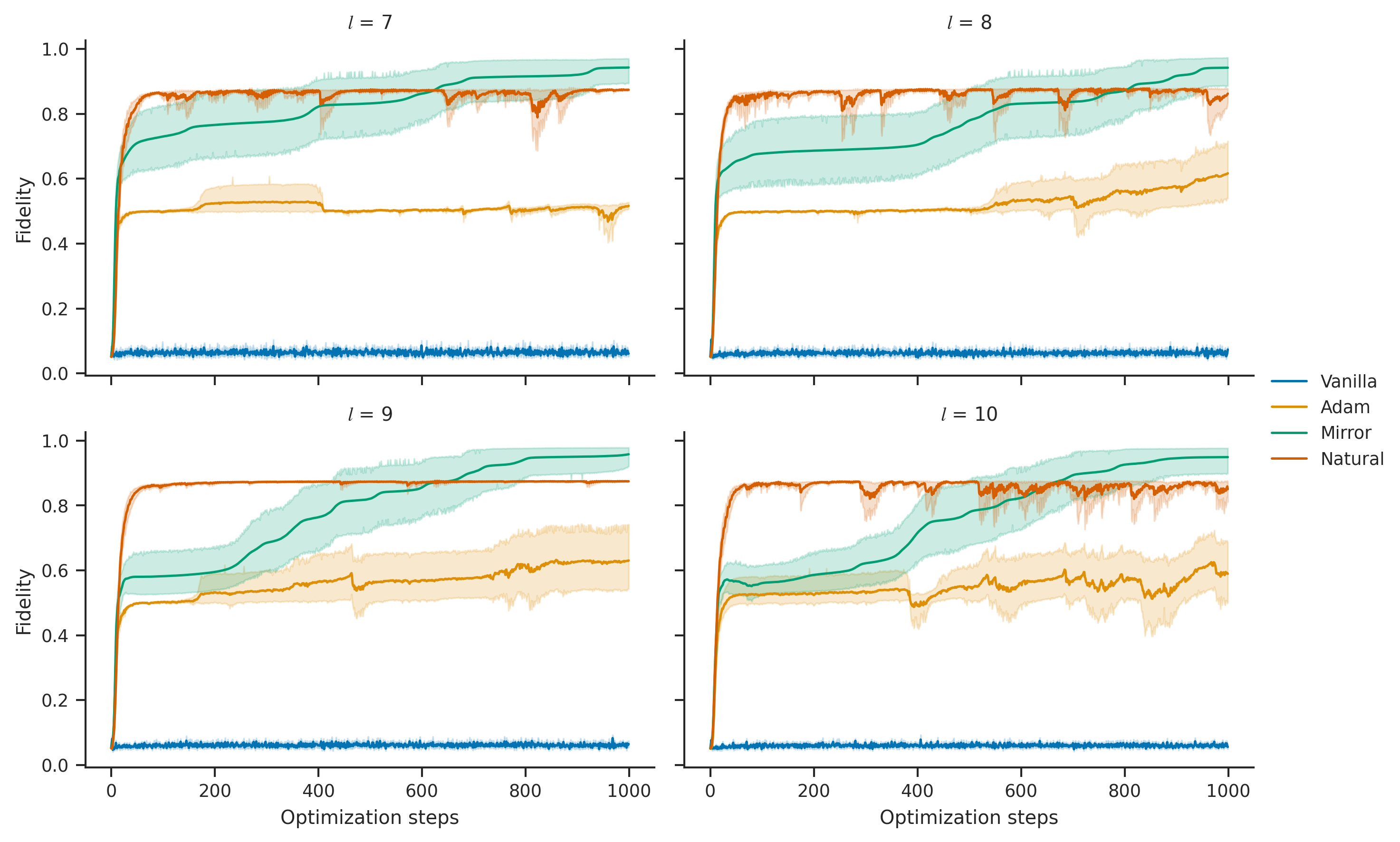
The TFIM is a simplified model of many important physical systems stinchcombe1973ising. The Hamiltonian of the model can be written as
| (14) |
where and are the X and Z single-qubit Pauli operators acting on the th qubit, are parameters chosen to model the system of interest, and indexes pairs of qubits on some lattice. The classical limit was originally introduced to study ferromagnetic phase transitions lenz1920beitrag; ising1924beitrag; ising2017fate. The quantized version was introduced by Heisenberg heisenberg1928theorie. It has since been used to calculate properties of many physical systems displaying ferromagnetism, such as ferroelectric crystals blinc1960isotopic; de1963collective and rare earth magnets wang1968collective. In these settings, depends on the distance between lattice sites in the crystal and depends on the tunneling frequency of the particles between sites.
In this section we study the equilibrium properties of the TFIM using a simulation of quantum Gibbs sampling. More specifically, given an inverse temperature , the task is to simulate the associated thermal state
| (15) |
We choose a QHBM as our ansatz and train it to represent using the free energy as our loss function3434 34 This makes our strategy an instance of VQT, see Section G.1.1. Equivalently, we minimize the forward quantum relative entropy .
For our investigation we choose the target Hamiltonian to be equation (15) on a six qubit chain. We choose , which is the quantum critical point of the system elliott1970ising; we choose a quantum critical point because these points often have rich entanglement structure and high quantum complexity osborne2002entanglement. For our model we choose our unitary to be a QHEA with layers and our energy function to be a fully connected Boltzmann machine. We compare four different optimizers for minimizing the free energy loss: SGD, Adam, QPNGD (Algorithm 1), and QPMD (Algorithm 2). We also test four different ansatz depths.
The results are shown in Footnote 33. We see that both of our proposed algorithms, QPNGD and QPMD, outperform Adam (which does not converge usefully) while using a fixed resource of data samples per iteration. While QPNGD ascends more quickly to a high fidelity, it jitters at a suboptimal fidelity. In constrast, we see that QPMD smoothly ascends to the optimum, despite using fewer model samples per iteration than QPNGD. As motivated theoretically in Section V, QPMD can be considered a (model) sample-efficient approximation to QPNGD. In fact, Adam can be understood as an approximate version of classical Natural Gradient Descent (NGD) leveraging an online estimator of the diagonal elements of the metric kingma2014adam.
VII Efficient generative modeling of quantum-stochastic processes

Quantum Fisher efficiency is an asymptotic result and so may bring untenable constant factors. From the proof, for a finite number of optimization steps, fast convergence in the error covariance occurs in the neighborhood where the loss is well-approximated by a convex quadratic function (Section VII.3). For this reason, initialization strategies which begin the optimization in proximity to the optimum would help achieve practical performance for many tasks of interest. As we motivate below, there are families of practical scenarios, which can be summarized as the modeling of sequences of mixed states that lie on a continuous path in some task space, which are conducive to a simple initialization strategy: initializing parameters at the optimum of the previous element in the task sequence. We call this chained initialization. As we demonstrate empirically below, this strategy is advantageous (Section VII.1) for simulations of both real and imaginary time evolution, amongst other potential applications.
VII.1 Sequences of States
Often, one wishes to model the equilibrium distribution of a quantum system as certain parameters of the target Hamiltonian are continuously modified. One such scenario is molecular geometry optimization, where parameters in the Hamiltonian represent inter-particle distances. The goal is to minimize the free energy with respect to those parameters, to find what configuration the molecule takes on in thermal equilibrium nagaoka2003structure. Another scenario is quantum annealing, where we wish to reach equilibrium as a parameter of the Hamiltonian is continuously tuned apolloni1989quantum; apolloni1990numerical; finnila1994quantum. A valid schedule can be constructed using measurements at multiple parameter points, using for example the Bashful Adiabatic Algorithm jarret2018quantum. From a learning perspective, if one has quantum measurement access to a physical system, then one may wish to learn a generative model of that system as some physical parameter is continuously varied. One such scenario is learning the entanglement Hamiltonian of a quantum field during time evolution wen2018entanglement.
For such parametric families of tasks and sufficiently fine evolution, neighboring target states may be expected to be close to one another according to the metric over . On the other hand, their distance in parameter space may be arbitrarily far. Hence, optimizers such as Adam which are unaware of the metric may not meaningfully benefit from initializing model parameters at the previous optimum. However, through a basic chaining of QPMD optimization loops, we can leverage their adjacency on while continuing not to refer explicitly to the Euclidean parameter space.
Concretely, suppose we have a parameterization of a task space. The task parameters (which could be target Hamiltonian parameters, time, temperature, or others) specify the target state . Suppose we are interested in a path in this space of parameters where . We can consider a partitioning of the path which gives the sequence of target states . We wish to learn a sequence of parameters so that for each .
Assuming the aforementioned geometric locality between neighboring states motivates our initialization strategy. Having trained model in the sequence, we simply propose initializing the parameters of the next model at at the start of its optimization. We call this chained initialization, written explicitly in Algorithm 3 (Section J.2). We can view this as a straightforward meta-learning for initialization nichol2018first; verdon2019learning technique.
VII.1.1 Numerical results
To test this initialization strategy numerically, we consider a simulation scenario for a sequence of states. In particular, we consider a sequence of thermal states defined by discretely varying the inverse temperature in (15) from to . This means the sequence of target states undergoes a cooling process, also known as imaginary or Wick-rotated time evolution goldberg1967integration. We additionally fix . As our model for the system at each temperature, we choose a QHBM with seven QHEA layers. This depth was chosen because it was found to be sufficient when learning the temperature in Footnote 33. Similarly, the energy function is chosen to be a fully connected Boltzmann machine.
In Figure 5a, we compare two different initialization strategies across two different optimization algorithms, applied to the cooling process described above. The “independent” row in each subfigure corresponds to randomly initializing the parameters of the model at each temperature step, while “chained” corresponds to initializing the parameters at the previous optimum. For both tested optimization algorithms, Adam and QPMD, chained initialization helps find better optima. We see that QPMD outperforms Adam under either initialization strategy, corroborating the benefits seen in Footnote 33. Figures displaying full training curves and confidence intervals at each temperature step can be found in the appendix (Figure 8). Again, chaining is particularly useful here when combined with QPMD because it is aware of locality between neighboring states in the sense of statistical distance. Indeed, neighboring states may be arbitrarily far in parameter space and so initialization at the previous optimum is not sufficient for other optimizers (such as Adam) which are unaware of the fundamental statistical distance.


VII.2 Sequences of Maps
In the previous section, we talked about simulating and learning sequences of Hamiltonians. In this section, we describe a different scenario: simulating the evolution of an initial state under a known mapping. Such mappings are one realization of quantum-stochastic processes3535 35 See Section J.1 for background material on open quantum system time evolution. milz2021quantum.
Calculating the time evolution of quantum systems is an important problem in physics abrams1997simulation and chemistry kassal2008polynomial; mcardle2020quantum, and it is known that time evolution of both open and closed quantum systems could be simulated efficiently using quantum computers lloyd1996universal; kliesch2011dissipative. Given a Hamiltonian , the formulas of Trotter trotter1959product and Suzuki suzuki1976generalized inform how to approximately time evolve states under on a quantum computer nielsen2010quantum. However, the resulting quantum circuits grow linearly with the simulation time, making them infeasible to implement on near term hardware.
Here, we describe an approach whose circuit depth does not grow with time. Suppose we are given access to copies of an initial quantum state and a known quantum channel that applies an open quantum system evolution for time . Our goal is then to simulate the evolution of the initial quantum state under the action of up to some final simulation time .
We could naively use quantum channel Trotter decomposition to simulate kliesch2011dissipative, but this would take circuit depth scaling with . Instead, suppose we discretize into a sequence of short time evolutions for . We now define a recursive algorithm in terms of these shorter channels. Assume we can generate copies of the learned state at step (for , this is simply the initial state ). Then we can apply the th channel to samples from , and train the next model against it using the reverse relative entropy loss. The resulting optimized state then serves as approximation of the true evolved state,
| (16) |
We may intuitively view this approach as checkpointing3636 36 We generalize to sequences of CPTP maps and provide more background in Section J.5. Pseudocode for the generalized form is given in Algorithm 4. of the quantum dynamics of a system relative to an initial state, saving the the information in the classical parameters of a model. As a result, our quantum circuit depth requirements can remain constant with respect to , assuming a fixed upper bound to the quantum complexity haferkamp2022linear of states along the trajectory. We refer to this approach as Quantum Variational Recursive Time Evolution AnsatZe (QVARTZ).
Other variational approaches exist for simulating time evolution. One promising method, called Variational Fast Forwarding (VFF), uses quantum compilation to learn a diagonalized ansatz for the time evolution operator cirstoiu2020variational. Like checkpointing, the circuit depth of VFF is fixed independently of . However, often one is only interested in applying time dynamics to a limited set of initial states. We hypothesize that learning the dynamics for all possible input states is generally more difficult than learning the dynamics of a few specific input states; in this case checkpointing may have an advantage over VFF. In another approach, a differential equation for the time evolution of the parameters of the model circuit is developed li2017efficient; then, a quantum computer is used to calculate terms in the differential equation, while a classical computer performs the integration. The checkpointing approach we described above has previously been proposed for pure states lin2021real; benedetti2021hardware.
VII.2.1 Numerical results
We test our approach by applying unitary time evolution to a mixed initial state. We take the initial state to be the Gibbs state corresponding to the TFIM Hamiltonian in equation (14). We choose the same parameters as in the equilibrium numerics of Footnote 33: , , but now supported on a chain of four qubits. To enable querying the initial state and evolving it through time, we start each trial of the experiment by training a QHBM via VQT against the Hamiltonian.
For our time evolution we choose a uniform partition with , such that and (we work in nondimensional units). Next, recall the TFIM Hamiltonian in Equation 14. We set up two independent Gaussian processes, and , with exponential quadratic kernels3737 37 From the TFP documentation, we have . We used for both the and processes.. We sample each process once for each time interval , yielding sequences and for the parameters, and for the time interval lengths. Letting be the TFIM Hamiltonian with and , our chosen time evolution operator during the interval was . We approximate this evolution using Trotterization. In summary, the sequence of channels mimics time evolution under a low frequency noise applied to the equilibrium Hamiltonian.
In Figure 5b we compare random initialization against chained initialization under optimization with either Adam or QPMD. Chained initialization helps find better optima under both optimizers. We also see that QPMD outperforms Adam under either initialization strategy, similar to the results in Figure 5a. Figures displaying full training curves and confidence intervals at each temperature step can be found in the appendix (Figure 9).
VII.3 Tuning Path Discretization Fineness
In both the state and map sequence scenarios, there is still the question of choosing appropriate step sizes in the task parameter (e.g. in the case of imaginary time evolution).
We recognize that Theorem IV.1 is asymptotic. Hence, for a finite and small number of optimization steps, convergence in the error covariance may not be meaningfully efficient. However, from the proof of the theorem, the neighborhood of the optimal parameters for which the asymptotic quantum Fisher efficiency (QFE) holds is a region for which the loss converges to a convex quadratic function sufficiently quickly so that, as a necessary condition3838 38 See Section D.3.1.,
| (17) |
for all where is a finite constant, and where is the Frobenius norm. Hence, since the chained initialization introduced in Section VII.1 involves initialization at the previous optimum, , it is natural to prefer a path discretization which satisfies
| (18) |
for some sufficiently small that evidently controls the constant factor in (17), and so serves as a useful empirical indicator.
To select a task space discretization which meets this initialization criteria it is then necessary to be able to translate from task space to model space coordinates. To this end, we work out the relevant expressions specific to real-time evolution, imaginary time-evolution, and generalizations of the latter to any generic path in parametric mixed state space in Appendix L.
VIII Discussion & Outlook
In this paper, we have discussed a general variational algorithm, QPNGD, for learning and simulating quantum Gibbs states. This algorithm is a generalization of metric-aware descent to quantum. However, we showed that a specific choice of metric (the BKM i.e. Hessian of self-relative entropy) that had not been discussed in prior work on optimization leads to several interesting properties; extending any of these results to additional choices of metric is of interest.
For one, we showed that, for general ansatze, this choice leads to an asymptotic optimality termed quantum Fisher efficiency. This is a novel result for quantum variational algorithms and is analogous to a celebrated classical result amari1998natural. It describes convergence as a function of data samples in terms of optimal parameter estimation. We suggested extending the applicability of this result, for example to non-convex landscapes and over-parameterized models, as an interesting follow-up with classical precedent martens2014new.
As an application of our quantum Fisher efficiency result, we studied the theoretically and experimentally popular quantum Hamiltonian learning problem swingle2014reconstructing; bairey2019learning; qi2019determining; evans2019scalable; anshu2021sample; haah2021optimal; anshu2022some; wang2017experimental; senko2014coherent and observed that we recover an any-temperature sample-efficient scaling akin to the best-known one of Anshu et al. anshu2021sample. We discussed an analogous scaling result for the ubiquitous Gibbs sampling (simulation) task feynman1982simulating; lloyd1996universal; kassal2011simulating; lloyd2014quantum; montanaro2015quantum; dallaire2016method; brandao2017quantum; brandao2019quantum; arute2019quantum; van2019improvements; motta2019qite; cohn2020minimal; van2020quantum; bauer2020quantum; harrow2020adaptive; sun2021qite; brandao2022faster, the first-known guarantee of its kind to be stated. Improving our complexity analysis is a desirable follow-up. Finding further applications of quantum Fisher efficiency is also of interest.
Furthermore, we distinguished data samples from model samples and noted that our update rule (QPNGD) may be costly in terms of number of model thermal state preparations. Hence, again for the same choice of metric, we established a dual first-order algorithm (QPMD) which approximates the same underlying coordinate-invariant flow. This extended two popular results in the classical literature raskutti2015information; gunasekar2021mirrorless to the realm of quantum machine learning.
We leveraged the fact that this metric indicates such a coordinate-invariant flow to suggest carrying over the aforementioned sample-efficiency result to an ansatz amenable to computational efficiency improvements and that acts as a re-parameterization of the same model subset of . We discussed in depth the QHBM ansatz which, through diagonalization, can translate the relevant thermal sampling problem to be classical instead of quantum, thus opening to expected exponential time complexity advantages for broad problem classes (for example, under the ETH assumption). Hence, this prescribes a general approach which makes headway into the wide-open question anshu2022some of practical algorithms for quantum Hamiltonian learning that are both time- and sample-efficient. Theoretical investigation into specific problem instances and variational diagonal ansatze which admit such advantage are desired.
Having designed and analyzed our main algorithm and its tractable approximation, we then identified, in connection with asymptotic quantum Fisher efficiency, a broad class of scenarios where non-asymptotic convergence may be fast. This class of scenarios is either learning or simulating sequences of quantum Gibbs states, where the states in the sequence are in information-geometric proximity. Such proximity allows metric-aware optimizers like QPMD to take advantage of the simple strategy of initializing at the previous optimum. Sequence scenarios can arise by varying the inverse temperature or the Hamiltonian parameters of a target Gibbs state, or by tracking quantum states through open or closed time evolutions.
For inference on sequences of maps, checkpointing (QVARTZ) converts a problem whose circuit depth scales linearly with time into a problem whose circuit depth saturates at the quantum complexity of the evolved state itself. This motivates further study of the learnability and representability of quantum states generated by low-depth quantum circuits farhi2014quantum; peruzzo2014variational; bravyi2018quantum; cerezo2021variational; haferkamp2022linear; brandao2021models. We believe our approach to time evolution, coupled with quantum neural architecture search methods zhang2020differentiable; du2020quantum; bilkis2021semi; li2020quantum, may enable the estimation of the quantum complexity of states during time evolution, a topic of central interest in the study of quantum gravity brown2018second; brown2017quantum; stanford2014complexity; brown2015complexity; susskind2020three; brown2016complexity; susskind2018black and holographic condensed matter theory jian2021complexity; das2017three.
In our numerics, we observed a particularly strong characteristic to QPMD, and strong performance advantage for sequences, tying together all of the theoretical results discussed above. Further studies into more complex, and especially the higher-difficulty non-stoquastic bravyi2014monte many-body systems would be desirable. To tackle such harder classes of Hamiltonians, numerical studies which invoke ansatze (which may be specific instances of QHBMs) that are non-trivially time-efficient in their optimization for specific problem instances are of interest.
Note that simulations presented in this paper were all assuming noiseless quantum computations. For further extensions of this work, we plan to address this limitation by exploring ways to extrapolate and interpolate state paths via representations of quantum dynamical maps as flows in model parameter space, potentially yielding novel variants of fast-forwarding and error mitigation van2022probabilistic strategies which are native to our quantum-probabilistic representations. Demonstrating the effectiveness of such a quantum-probabilistic error mitigation scheme would be a stepping stone towards a real-world experimental demonstration of quantum advantage for time evolution via QVARTZ on a noisy, near-term device preskill2018quantum; preskill2021quantum, an objective for future work.
For our core proofs, consistent with the literature taken as baseline, we assumed strong inductive biases in our model which matched quite tightly the physical scenario at hand (though discussed that relaxation is feasible with our approach). In realistic scenarios, one often knows symmetries or general properties of the system, but not the exact space spanned by the Hamiltonian parameterization. As such, explorations of ansatze with physical-context-aware inductive biases are of interest to ensure time efficiency for scenarios with less sharp priors over the Hamiltonian structure. To this end, recent advances towards a theory of quantum geometric deep learning verdon2019quantum; larocca2022group; meyer2022exploiting are interesting directions in which to extent our current framework.
Acknowledgements.
We thank James Martens, Marcin Jarzyna, Josh Dillon, Will Grathwohl, Thomas Wang, Trevor McCourt, and Patrick Coles for helpful discussions. We thank Joshua Greenberg for artistic illustrations. All numerical simulations in this paper were performed using our open source QHBM library3939 39 Accessible at https://github.com/google/qhbm-library., built on a combination of TensorFlow Quantum broughton2020tensorflow and TensorFlow Probability dillon2017tensorflow. X, formerly known as Google[x], is part of the Alphabet family of companies, which includes Google, Verily, Waymo, and others (www.x.company).References
- [1] Anurag Anshu. Some recent progress in learning theory: The quantum side. Harvard Data Science Review, 2022.
- [2] Michael Broughton, Guillaume Verdon, Trevor McCourt, Antonio J Martinez, Jae Hyeon Yoo, Sergei V Isakov, Philip Massey, Ramin Halavati, Murphy Yuezhen Niu, Alexander Zlokapa, et al. Tensorflow quantum: A software framework for quantum machine learning. arXiv preprint arXiv:2003.02989, 2020.
- [3] Yazhen Wang. When quantum computation meets data science: Making data science quantum. Harvard Data Science Review, 2022.
- [4] Aram W Harrow, Avinatan Hassidim, and Seth Lloyd. Quantum algorithm for linear systems of equations. Physical review letters, 103(15):150502, 2009.
- [5] Ewin Tang. Quantum principal component analysis only achieves an exponential speedup because of its state preparation assumptions. Physical Review Letters, 127(6):060503, 2021.
- [6] Ewin Tang. A quantum-inspired classical algorithm for recommendation systems. In Proceedings of the 51st Annual ACM SIGACT Symposium on Theory of Computing, pages 217–228, 2019.
- [7] Jarrod R McClean, Sergio Boixo, Vadim N Smelyanskiy, Ryan Babbush, and Hartmut Neven. Barren plateaus in quantum neural network training landscapes. Nature communications, 9(1):4812, 2018.
- [8] Samson Wang, Enrico Fontana, Marco Cerezo, Kunal Sharma, Akira Sone, Lukasz Cincio, and Patrick J Coles. Noise-induced barren plateaus in variational quantum algorithms. Nature communications, 12(1):1–11, 2021.
- [9] Vittorio Giovannetti, Seth Lloyd, and Lorenzo Maccone. Quantum random access memory. Physical review letters, 100(16):160501, 2008.
- [10] Scott Aaronson. Read the fine print. Nature Physics, 11(4):291–293, 2015.
- [11] Yunchao Liu, Srinivasan Arunachalam, and Kristan Temme. A rigorous and robust quantum speed-up in supervised machine learning. Nature Physics, 17(9):1013–1017, 2021.
- [12] Srinivasan Arunachalam and Ronald de Wolf. Guest column: A survey of quantum learning theory. ACM SIGACT News, 48(2):41–67, 2017.
- [13] Srinivasan Arunachalam, Alex B Grilo, Tom Gur, Igor C Oliveira, and Aarthi Sundaram. Quantum learning algorithms imply circuit lower bounds. In 2021 IEEE 62nd Annual Symposium on Foundations of Computer Science (FOCS), pages 562–573. IEEE, 2022.
- [14] Scott Aaronson. Shadow tomography of quantum states. SIAM Journal on Computing, 49(5):STOC18–368, 2019.
- [15] Hsin-Yuan Huang, Richard Kueng, and John Preskill. Predicting many properties of a quantum system from very few measurements. Nature Physics, 16(10):1050–1057, 2020.
- [16] Hsin-Yuan Huang, Michael Broughton, Jordan Cotler, Sitan Chen, Jerry Li, Masoud Mohseni, Hartmut Neven, Ryan Babbush, Richard Kueng, John Preskill, et al. Quantum advantage in learning from experiments. arXiv preprint arXiv:2112.00778, 2021.
- [17] Hsin-Yuan Huang, Richard Kueng, and John Preskill. Information-theoretic bounds on quantum advantage in machine learning. Physical Review Letters, 126(19):190505, 2021.
- [18] Hsin-Yuan Huang, Richard Kueng, Giacomo Torlai, Victor V Albert, and John Preskill. Provably efficient machine learning for quantum many-body problems. arXiv preprint arXiv:2106.12627, 2021.
- [19] Frank Arute, Kunal Arya, Ryan Babbush, Dave Bacon, Joseph C Bardin, Rami Barends, Rupak Biswas, Sergio Boixo, Fernando GSL Brandao, David A Buell, et al. Quantum supremacy using a programmable superconducting processor. Nature, 574(7779):505–510, 2019.
- [20] K Vogel and H Risken. Determination of quasiprobability distributions in terms of probability distributions for the rotated quadrature phase. Physical Review A, 40(5):2847, 1989.
- [21] Fernando G. S. L. Brandão, Amir Kalev, Tongyang Li, Cedric Yen-Yu Lin, Krysta M. Svore, and Xiaodi Wu. Quantum SDP Solvers: Large Speed-Ups, Optimality, and Applications to Quantum Learning. In Christel Baier, Ioannis Chatzigiannakis, Paola Flocchini, and Stefano Leonardi, editors, 46th International Colloquium on Automata, Languages, and Programming (ICALP 2019), volume 132 of Leibniz International Proceedings in Informatics (LIPIcs), pages 27:1–27:14, Dagstuhl, Germany, 2019. Schloss Dagstuhl–Leibniz-Zentrum fuer Informatik.
- [22] Mario Szegedy. Quantum speed-up of markov chain based algorithms. In 45th Annual IEEE symposium on foundations of computer science, pages 32–41. IEEE, 2004.
- [23] Man-Hong Yung and Alán Aspuru-Guzik. A quantum–quantum metropolis algorithm. Proceedings of the National Academy of Sciences, 109(3):754–759, 2012.
- [24] Anurag Anshu, Srinivasan Arunachalam, Tomotaka Kuwahara, and Mehdi Soleimanifar. Sample-efficient learning of interacting quantum systems. Nature Physics, 17(8):931–935, 2021.
- [25] Jeongwan Haah, Robin Kothari, and Ewin Tang. Optimal learning of quantum hamiltonians from high-temperature gibbs states. arXiv preprint arXiv:2108.04842, 2021.
- [26] Jing Liu, Haidong Yuan, Xiao-Ming Lu, and Xiaoguang Wang. Quantum fisher information matrix and multiparameter estimation. Journal of Physics A: Mathematical and Theoretical, 53(2):023001, 2019.
- [27] Brian Swingle and Isaac H Kim. Reconstructing quantum states from local data. Physical review letters, 113(26):260501, 2014.
- [28] Eyal Bairey, Itai Arad, and Netanel H Lindner. Learning a local hamiltonian from local measurements. Physical review letters, 122(2):020504, 2019.
- [29] Xiao-Liang Qi and Daniel Ranard. Determining a local hamiltonian from a single eigenstate. Quantum, 3:159, 2019.
- [30] Tim J Evans, Robin Harper, and Steven T Flammia. Scalable bayesian hamiltonian learning. arXiv preprint arXiv:1912.07636, 2019.
- [31] Jianwei Wang, Stefano Paesani, Raffaele Santagati, Sebastian Knauer, Antonio A Gentile, Nathan Wiebe, Maurangelo Petruzzella, Jeremy L O’Brien, John G Rarity, Anthony Laing, et al. Experimental quantum hamiltonian learning. Nature Physics, 13(6):551–555, 2017.
- [32] C Senko, J Smith, P Richerme, A Lee, WC Campbell, and C Monroe. Coherent imaging spectroscopy of a quantum many-body spin system. Science, 345(6195):430–433, 2014.
- [33] Christian Kokail, Rick van Bijnen, Andreas Elben, Benoît Vermersch, and Peter Zoller. Entanglement hamiltonian tomography in quantum simulation. Nature Physics, 17(8):936–942, 2021.
- [34] Marcello Dalmonte, Viktor Eisler, Marco Falconi, and Benoıt Vermersch. Entanglement hamiltonians: from field theory, to lattice models and experiments. arXiv preprint arXiv:2202.05045, 2022.
- [35] Nicolas Regnault. Entanglement spectroscopy and its application to the quantum hall effects. Lecture Notes Les Houches Summer School, 103:165, 2017.
- [36] Rudolf Haag. Local quantum physics: Fields, particles, algebras. Springer Science & Business Media, 2012.
- [37] Horacio Casini, Marina Huerta, and Robert C Myers. Towards a derivation of holographic entanglement entropy. Journal of High Energy Physics, 2011(5):1–41, 2011.
- [38] CKCN Chow and Cong Liu. Approximating discrete probability distributions with dependence trees. IEEE transactions on Information Theory, 14(3):462–467, 1968.
- [39] Geoffrey E Hinton et al. Learning distributed representations of concepts. In Proceedings of the eighth annual conference of the cognitive science society, volume 1, page 12. Amherst, MA, 1986.
- [40] David R Karger and Nathan Srebro. Learning markov networks: maximum bounded tree-width graphs. In SODA, volume 1, pages 392–401, 2001.
- [41] Pieter Abbeel, Daphne Koller, and Andrew Y Ng. Learning factor graphs in polynomial time and sample complexity. The Journal of Machine Learning Research, 7:1743–1788, 2006.
- [42] Narayana P Santhanam and Martin J Wainwright. Information-theoretic limits of selecting binary graphical models in high dimensions. IEEE Transactions on Information Theory, 58(7):4117–4134, 2012.
- [43] Guy Bresler, Elchanan Mossel, and Allan Sly. Reconstruction of markov random fields from samples: Some observations and algorithms. In Approximation, Randomization and Combinatorial Optimization. Algorithms and Techniques, pages 343–356. Springer, 2008.
- [44] Guy Bresler. Efficiently learning ising models on arbitrary graphs. In Proceedings of the forty-seventh annual ACM symposium on Theory of computing, pages 771–782, 2015.
- [45] Marc Vuffray, Sidhant Misra, Andrey Lokhov, and Michael Chertkov. Interaction screening: Efficient and sample-optimal learning of ising models. Advances in neural information processing systems, 29, 2016.
- [46] Adam Klivans and Raghu Meka. Learning graphical models using multiplicative weights. In 2017 IEEE 58th Annual Symposium on Foundations of Computer Science (FOCS), pages 343–354. IEEE, 2017.
- [47] Nihal Yapage and Hiroshi Nagaoka. An information geometrical approach to the mean-field approximation for quantum ising spin models. Journal of Physics A: Mathematical and Theoretical, 41(6):065005, 2008.
- [48] Patrik Henelius and Anders W Sandvik. Sign problem in monte carlo simulations of frustrated quantum spin systems. Physical Review B, 62(2):1102, 2000.
- [49] Dominik Hangleiter, Ingo Roth, Daniel Nagaj, and Jens Eisert. Easing the monte carlo sign problem. Science Advances, 6(33):eabb8341, 2020.
- [50] Aram W Harrow, Saeed Mehraban, and Mehdi Soleimanifar. Classical algorithms, correlation decay, and complex zeros of partition functions of quantum many-body systems. In Proceedings of the 52nd Annual ACM SIGACT Symposium on Theory of Computing, pages 378–386, 2020.
- [51] Josh M Deutsch. Quantum statistical mechanics in a closed system. Physical review a, 43(4):2046, 1991.
- [52] Mark Srednicki. Chaos and quantum thermalization. Physical review e, 50(2):888, 1994.
- [53] Richard P Feynman. Simulating physics with computers. Int. J. Theor. Phys, 21(6/7), 1982.
- [54] S Lloyd. Universal quantum simulators. Science, 273(5278):1073–1078, August 1996.
- [55] Ivan Kassal, James D Whitfield, Alejandro Perdomo-Ortiz, Man-Hong Yung, and Alán Aspuru-Guzik. Simulating chemistry using quantum computers. Annual review of physical chemistry, 62:185–207, 2011.
- [56] Mario Motta, Chong Sun, Adrian T K Tan, Matthew J O’Rourke, Erika Ye, Austin J Minnich, Fernando G S, and Garnet Kin-Lic Chan. Determining eigenstates and thermal states on a quantum computer using quantum imaginary time evolution. Nat. Phys., 16(2):205–210, November 2019.
- [57] Pierre-Luc Dallaire-Demers and Frank K Wilhelm. Method to efficiently simulate the thermodynamic properties of the fermi-hubbard model on a quantum computer. Physical Review A, 93(3):032303, 2016.
- [58] Jeffrey Cohn, F Yang, K Najafi, Barbara Jones, and James K Freericks. Minimal effective gibbs ansatz: A simple protocol for extracting an accurate thermal representation for quantum simulation. Physical Review A, 102(2):022622, 2020.
- [59] Shi-Ning Sun, Mario Motta, Ruslan N Tazhigulov, Adrian T K Tan, Garnet Kin-Lic Chan, and Austin J Minnich. Quantum computation of finite-temperature static and dynamical properties of spin systems using quantum imaginary time evolution. PRX Quantum, 2(1), February 2021.
- [60] Bela Bauer, Sergey Bravyi, Mario Motta, and Garnet Kin-Lic Chan. Quantum algorithms for quantum chemistry and quantum materials science. Chemical Reviews, 120(22):12685–12717, 2020.
- [61] Fernando GSL Brandao and Krysta M Svore. Quantum speed-ups for solving semidefinite programs. In 2017 IEEE 58th Annual Symposium on Foundations of Computer Science (FOCS), pages 415–426. IEEE, 2017.
- [62] Joran van Apeldoorn and András Gilyén. Improvements in Quantum SDP-Solving with Applications. In Christel Baier, Ioannis Chatzigiannakis, Paola Flocchini, and Stefano Leonardi, editors, 46th International Colloquium on Automata, Languages, and Programming (ICALP 2019), volume 132 of Leibniz International Proceedings in Informatics (LIPIcs), pages 99:1–99:15, Dagstuhl, Germany, 2019. Schloss Dagstuhl–Leibniz-Zentrum fuer Informatik.
- [63] Joran Van Apeldoorn, András Gilyén, Sander Gribling, and Ronald de Wolf. Quantum sdp-solvers: Better upper and lower bounds. Quantum, 4:230, 2020.
- [64] Fernando GS L Brandao, Richard Kueng, and Daniel Stilck França. Faster quantum and classical sdp approximations for quadratic binary optimization. Quantum, 6:625, 2022.
- [65] Ashley Montanaro. Quantum speedup of monte carlo methods. Proceedings of the Royal Society A: Mathematical, Physical and Engineering Sciences, 471(2181):20150301, 2015.
- [66] Aram W Harrow and Annie Y Wei. Adaptive quantum simulated annealing for bayesian inference and estimating partition functions. In Proceedings of the Fourteenth Annual ACM-SIAM Symposium on Discrete Algorithms, pages 193–212. SIAM, 2020.
- [67] Seth Lloyd, Masoud Mohseni, and Patrick Rebentrost. Quantum principal component analysis. Nature Physics, 10(9):631, 2014.
- [68] Garvesh Raskutti and Sayan Mukherjee. The information geometry of mirror descent. IEEE Transactions on Information Theory, 61(3):1451–1457, 2015.
- [69] Masataka Nagaoka. Structure optimization of solute molecules via free energy gradient method. Bulletin of the Korean Chemical Society, 24(6):805–808, 2003.
- [70] Bruno Apolloni, C Carvalho, and Diego De Falco. Quantum stochastic optimization. Stochastic Processes and their Applications, 33(2):233–244, 1989.
- [71] Bruno Apolloni, Nicolò Cesa-Bianchi, and Diego De Falco. A numerical implementation of “quantum annealing”. In Stochastic Processes, Physics and Geometry: Proceedings of the Ascona-Locarno Conference, pages 97–111, 1990.
- [72] Aleta Berk Finnila, MA Gomez, C Sebenik, Catherine Stenson, and Jimmie D Doll. Quantum annealing: A new method for minimizing multidimensional functions. Chemical physics letters, 219(5-6):343–348, 1994.
- [73] Daniel S Abrams and Seth Lloyd. Simulation of many-body fermi systems on a universal quantum computer. Physical Review Letters, 79(13):2586, 1997.
- [74] Ivan Kassal, Stephen P Jordan, Peter J Love, Masoud Mohseni, and Alán Aspuru-Guzik. Polynomial-time quantum algorithm for the simulation of chemical dynamics. Proceedings of the National Academy of Sciences, 105(48):18681–18686, 2008.
- [75] Sam McArdle, Suguru Endo, Alán Aspuru-Guzik, Simon C Benjamin, and Xiao Yuan. Quantum computational chemistry. Reviews of Modern Physics, 92(1):015003, 2020.
- [76] Nathan Wiebe, Christopher Granade, Christopher Ferrie, and David Cory. Quantum hamiltonian learning using imperfect quantum resources. Physical Review A, 89(4):042314, 2014.
- [77] Nathan Wiebe, Christopher Granade, Christopher Ferrie, and David G Cory. Hamiltonian learning and certification using quantum resources. Physical review letters, 112(19):190501, 2014.
- [78] Eyal Bairey, Chu Guo, Dario Poletti, Netanel H Lindner, and Itai Arad. Learning the dynamics of open quantum systems from their steady states. New Journal of Physics, 22(3):032001, 2020.
- [79] Julia Kempe, Alexei Kitaev, and Oded Regev. The complexity of the local hamiltonian problem. Siam journal on computing, 35(5):1070–1097, 2006.
- [80] Mohammad H Amin, Evgeny Andriyash, Jason Rolfe, Bohdan Kulchytskyy, and Roger Melko. Quantum boltzmann machine. Physical Review X, 8(2):021050, 2018.
- [81] Tzu-Chieh Wei, Michele Mosca, and Ashwin Nayak. Interacting boson problems are qma-hard. arXiv preprint arXiv:0905.3413, 2009.
- [82] Dorit Aharonov, Daniel Gottesman, Sandy Irani, and Julia Kempe. The power of quantum systems on a line. Communications in mathematical physics, 287(1):41–65, 2009.
- [83] Álvaro M Alhambra. Quantum many-body systems in thermal equilibrium. arXiv preprint arXiv:2204.08349, 2022.
- [84] Kristan Temme, Tobias J Osborne, Karl G Vollbrecht, David Poulin, and Frank Verstraete. Quantum metropolis sampling. Nature, 471(7336):87–90, 2011.
- [85] Kok Chuan Tan, Dhiman Bhowmick, and Pinaki Sengupta. Sign-problem free quantum stochastic series expansion algorithm on a quantum computer. npj Quantum Information, 8(1):1–7, 2022.
- [86] Guillaume Verdon, Jacob Marks, Sasha Nanda, Stefan Leichenauer, and Jack Hidary. Quantum hamiltonian-based models and the variational quantum thermalizer algorithm. arXiv preprint arXiv:1910.02071, 2019.
- [87] Chi-Fang Chen and Fernando GSL Brandão. Fast thermalization from the eigenstate thermalization hypothesis. arXiv preprint arXiv:2112.07646, 2021.
- [88] Ryan LaRose, Arkin Tikku, Étude O’Neel-Judy, Lukasz Cincio, and Patrick J Coles. Variational quantum state diagonalization. npj Quantum Information, 5(1):8, 2019.
- [89] M Cerezo, Kunal Sharma, Andrew Arrasmith, and Patrick J Coles. Variational quantum state eigensolver. arXiv preprint arXiv:2004.01372, 2020.
- [90] James Stokes, Josh Izaac, Nathan Killoran, and Giuseppe Carleo. Quantum natural gradient. Quantum, 4:269, 2020.
- [91] Bálint Koczor and Simon C Benjamin. Quantum natural gradient generalised to non-unitary circuits. arXiv preprint arXiv:1912.08660, 2019.
- [92] Barnaby van Straaten and Bálint Koczor. Measurement cost of metric-aware variational quantum algorithms. arXiv preprint arXiv:2005.05172, 2020.
- [93] Shun-Ichi Amari. Natural gradient works efficiently in learning. Neural computation, 10(2):251–276, 1998.
- [94] James Martens and Roger Grosse. Optimizing neural networks with kronecker-factored approximate curvature. In International conference on machine learning, pages 2408–2417. PMLR, 2015.
- [95] Jarrod R McClean, Jonathan Romero, Ryan Babbush, and Alán Aspuru-Guzik. The theory of variational hybrid quantum-classical algorithms. New Journal of Physics, 18(2):023023, 2016.
- [96] John Preskill. Quantum computing in the nisq era and beyond. Quantum, 2:79, 2018.
- [97] Marco Cerezo, Andrew Arrasmith, Ryan Babbush, Simon C Benjamin, Suguru Endo, Keisuke Fujii, Jarrod R McClean, Kosuke Mitarai, Xiao Yuan, Lukasz Cincio, et al. Variational quantum algorithms. Nature Reviews Physics, 3(9):625–644, 2021.
- [98] David Poulin, Angie Qarry, Rolando Somma, and Frank Verstraete. Quantum simulation of time-dependent hamiltonians and the convenient illusion of hilbert space. Physical review letters, 106(17):170501, 2011.
- [99] Ingemar Bengtsson and Karol Zyczkowski. Geometry of Quantum States. Cambridge University Press, Second Edition edition, 2017.
- [100] Kevin P Murphy. Machine learning: a probabilistic perspective. MIT press, 2012.
- [101] Dénes Petz. Covariance and fisher information in quantum mechanics. Journal of Physics A: Mathematical and General, 35(4):929, 2002.
- [102] Anna Jencová. Generalized relative entropies as contrast functionals on density matrices. International Journal of Theoretical Physics, 43(7):1635–1650, 2004.
- [103] J Pfanzagl. Asymptotic expansions related to minimum contrast estimators. The Annals of Statistics, pages 993–1026, 1973.
- [104] Shinto Eguchi. Second order efficiency of minimum contrast estimators in a curved exponential family. The Annals of Statistics, pages 793–803, 1983.
- [105] Aram W. Harrow and John C. Napp. Low-depth gradient measurements can improve convergence in variational hybrid quantum-classical algorithms. Phys. Rev. Lett., 126:140502, Apr 2021.
- [106] Theodore Frankel. The Geometry of Physics. Cambridge University Press, Third edition, 2012.
- [107] Mark M. Wilde. Quantum Information Theory. Cambridge University Press, Second Edition edition, 2017.
- [108] Andrew Lesniewski and Mary Beth Ruskai. 4. Journal of Mathematical Physics, 40(11):5702–5724, 1999.
- [109] Nikolai Nikolaevich Cencov. Statistical decision rules and optimal inference. American Mathematical Soc., 2000.
- [110] Shun-ichi Amari. Information geometry and its applications, volume 194. Springer, 2016.
- [111] Tengyuan Liang, Tomaso Poggio, Alexander Rakhlin, and James Stokes. Fisher-rao metric, geometry, and complexity of neural networks. In The 22nd International Conference on Artificial Intelligence and Statistics, pages 888–896. PMLR, 2019.
- [112] Allan Sly. Computational transition at the uniqueness threshold. In 2010 IEEE 51st Annual Symposium on Foundations of Computer Science, pages 287–296. IEEE, 2010.
- [113] Allan Sly and Nike Sun. The computational hardness of counting in two-spin models on d-regular graphs. In 2012 IEEE 53rd Annual Symposium on Foundations of Computer Science, pages 361–369. IEEE, 2012.
- [114] James Martens. New insights and perspectives on the natural gradient method. arXiv preprint arXiv:1412.1193, 2014.
- [115] Arthur Jacot, Franck Gabriel, and Clément Hongler. Neural tangent kernel: Convergence and generalization in neural networks. arXiv preprint arXiv:1806.07572, 2018.
- [116] Guodong Zhang, James Martens, and Roger Grosse. Fast convergence of natural gradient descent for overparameterized neural networks. arXiv preprint arXiv:1905.10961, 2019.
- [117] Tianle Cai, Ruiqi Gao, Jikai Hou, Siyu Chen, Dong Wang, Di He, Zhihua Zhang, and Liwei Wang. Gram-gauss-newton method: Learning overparameterized neural networks for regression problems. arXiv preprint arXiv:1905.11675, 2019.
- [118] Mária Kieferová and Nathan Wiebe. Tomography and generative training with quantum boltzmann machines. Physical Review A, 96(6):062327, 2017.
- [119] Christa Zoufal, Aurélien Lucchi, and Stefan Woerner. Variational quantum boltzmann machines. Quantum Machine Intelligence, 3(1):1–15, 2021.
- [120] Christian Kokail, Bhuvanesh Sundar, Torsten V Zache, Andreas Elben, Benoît Vermersch, Marcello Dalmonte, Rick van Bijnen, and Peter Zoller. Quantum variational learning of the entanglement hamiltonian. Physical review letters, 127(17):170501, 2021.
- [121] Anirban N Chowdhury, Guang Hao Low, and Nathan Wiebe. A variational quantum algorithm for preparing quantum gibbs states. arXiv preprint arXiv:2002.00055, 2020.
- [122] Emanuel Knill, Gerardo Ortiz, and Rolando D Somma. Optimal quantum measurements of expectation values of observables. Physical Review A, 75(1):012328, 2007.
- [123] Hiroshi Hasegawa. Exponential and mixture families in quantum statistics: Dual structure and unbiased parameter estimation. Reports on Mathematical Physics, 39(1):49–68, 1997.
- [124] Matheus R Grasselli and Raymond F Streater. On the uniqueness of the chentsov metric in quantum information geometry. Infinite Dimensional Analysis, Quantum Probability and Related Topics, 4(02):173–182, 2001.
- [125] Suriya Gunasekar, Blake Woodworth, and Nathan Srebro. Mirrorless mirror descent: A natural derivation of mirror descent. In International Conference on Artificial Intelligence and Statistics, pages 2305–2313. PMLR, 2021.
- [126] Barbara M Terhal and David P DiVincenzo. Problem of equilibration and the computation of correlation functions on a quantum computer. Physical Review A, 61(2):022301, 2000.
- [127] Daniel S Abrams and Seth Lloyd. Quantum algorithm providing exponential speed increase for finding eigenvalues and eigenvectors. Physical Review Letters, 83(24):5162, 1999.
- [128] David Poulin and Pawel Wocjan. Sampling from the thermal quantum gibbs state and evaluating partition functions with a quantum computer. Physical review letters, 103(22):220502, 2009.
- [129] Ersen Bilgin and Sergio Boixo. Preparing thermal states of quantum systems by dimension reduction. Physical review letters, 105(17):170405, 2010.
- [130] Arnau Riera, Christian Gogolin, and Jens Eisert. Thermalization in nature and on a quantum computer. Physical review letters, 108(8):080402, 2012.
- [131] Rolando D Somma and Sergio Boixo. Spectral gap amplification. SIAM Journal on Computing, 42(2):593–610, 2013.
- [132] Anirban Narayan Chowdhury and Rolando D Somma. Quantum algorithms for gibbs sampling and hitting-time estimation. arXiv preprint arXiv:1603.02940, 2016.
- [133] Michael J Kastoryano and Fernando GSL Brandao. Quantum gibbs samplers: The commuting case. Communications in Mathematical Physics, 344(3):915–957, 2016.
- [134] Yimin Ge, András Molnár, and J Ignacio Cirac. Rapid adiabatic preparation of injective projected entangled pair states and gibbs states. Physical review letters, 116(8):080503, 2016.
- [135] Fernando GSL Brandão and Michael J Kastoryano. Finite correlation length implies efficient preparation of quantum thermal states. Communications in Mathematical Physics, 365(1):1–16, 2019.
- [136] Erwin Schrödinger. An undulatory theory of the mechanics of atoms and molecules. Physical review, 28(6):1049, 1926.
- [137] AD McLachlan. A variational solution of the time-dependent schrodinger equation. Molecular Physics, 8(1):39–44, 1964.
- [138] J Broeckhove, L Lathouwers, E Kesteloot, and P Van Leuven. On the equivalence of time-dependent variational principles. Chemical physics letters, 149(5-6):547–550, 1988.
- [139] Sam McArdle, Tyson Jones, Suguru Endo, Ying Li, Simon C Benjamin, and Xiao Yuan. Variational ansatz-based quantum simulation of imaginary time evolution. npj Quantum Information, 5(1):1–6, 2019.
- [140] Steven R White. Minimally entangled typical quantum states at finite temperature. Physical review letters, 102(19):190601, 2009.
- [141] Frank Verstraete, Juan J Garcia-Ripoll, and Juan Ignacio Cirac. Matrix product density operators: Simulation of finite-temperature and dissipative systems. Physical review letters, 93(20):207204, 2004.
- [142] Michael Zwolak and Guifré Vidal. Mixed-state dynamics in one-dimensional quantum lattice systems: a time-dependent superoperator renormalization algorithm. Physical review letters, 93(20):207205, 2004.
- [143] Jochen Rau. Statistical physics and thermodynamics: an introduction to key concepts. Oxford University Press, 2017.
- [144] Jingxiang Wu and Timothy H Hsieh. Variational thermal quantum simulation via thermofield double states. Physical review letters, 123(22):220502, 2019.
- [145] Youle Wang, Guangxi Li, and Xin Wang. Variational quantum gibbs state preparation with a truncated taylor series. Physical Review Applied, 16(5):054035, 2021.
- [146] John Martyn and Brian Swingle. Product spectrum ansatz and the simplicity of thermal states. Physical Review A, 100(3):032107, 2019.
- [147] Jin-Guo Liu, Liang Mao, Pan Zhang, and Lei Wang. Solving quantum statistical mechanics with variational autoregressive networks and quantum circuits. Machine Learning: Science and Technology, 2(2):025011, 2021.
- [148] RB Stinchcombe. Ising model in a transverse field. i. basic theory. Journal of Physics C: Solid State Physics, 6(15):2459, 1973.
- [149] Wilhelm Lenz. Beitrag zum verständnis der magnetischen erscheinungen in festen körpern. Z. Phys., 21:613–615, 1920.
- [150] Ernst Ising. Beitrag zur theorie des ferro-und paramagnetismus. PhD thesis, Grefe & Tiedemann, 1924.
- [151] Thomas Ising, Reinhard Folk, Ralph Kenna, Bertrand Berche, and Yurij Holovatch. The fate of ernst ising and the fate of his model. arXiv preprint arXiv:1706.01764, 2017.
- [152] W Heisenberg. Zur theorie des ferromagnetismus. Zeitschrift für Physik, 49(9):619–636, 1928.
- [153] R Blinc. On the isotopic effects in the ferroelectric behavious of crystals with short hydrogen bonds. Phys. and Chem. Solids, 13, 1960.
- [154] PG De Gennes. Collective motions of hydrogen bonds. Solid State Communications, 1(6):132–137, 1963.
- [155] Yung-Li Wang and Bernard R Cooper. Collective excitations and magnetic ordering in materials with singlet crystal-field ground state. Physical Review, 172(2):539, 1968.
- [156] RJ Elliott, P Pfeuty, and C Wood. Ising model with a transverse field. Physical Review Letters, 25(7):443, 1970.
- [157] Tobias J Osborne and Michael A Nielsen. Entanglement in a simple quantum phase transition. Physical Review A, 66(3):032110, 2002.
- [158] Diederik P Kingma and Jimmy Ba. Adam: A method for stochastic optimization. arXiv preprint arXiv:1412.6980, 2014.
- [159] Michael Jarret, Brad Lackey, Aike Liu, and Kianna Wan. Quantum adiabatic optimization without heuristics. arXiv preprint arXiv:1810.04686, 2018.
- [160] Xueda Wen, Shinsei Ryu, and Andreas WW Ludwig. Entanglement hamiltonian evolution during thermalization in conformal field theory. Journal of Statistical Mechanics: Theory and Experiment, 2018(11):113103, 2018.
- [161] Alex Nichol, Joshua Achiam, and John Schulman. On first-order meta-learning algorithms. arXiv preprint arXiv:1803.02999, 2018.
- [162] Guillaume Verdon, Michael Broughton, Jarrod R McClean, Kevin J Sung, Ryan Babbush, Zhang Jiang, Hartmut Neven, and Masoud Mohseni. Learning to learn with quantum neural networks via classical neural networks. arXiv preprint arXiv:1907.05415, 2019.
- [163] Abraham Goldberg and Judah L Schwartz. Integration of the schrödinger equation in imaginary time. Journal of Computational Physics, 1(3):433–447, 1967.
- [164] Simon Milz and Kavan Modi. Quantum stochastic processes and quantum non-markovian phenomena. PRX Quantum, 2(3):030201, 2021.
- [165] Martin Kliesch, Thomas Barthel, Christian Gogolin, Michael Kastoryano, and Jens Eisert. Dissipative quantum church-turing theorem. Physical review letters, 107(12):120501, 2011.
- [166] Hale F Trotter. On the product of semi-groups of operators. Proceedings of the American Mathematical Society, 10(4):545–551, 1959.
- [167] Masuo Suzuki. Generalized trotter’s formula and systematic approximants of exponential operators and inner derivations with applications to many-body problems. Communications in Mathematical Physics, 51(2):183–190, 1976.
- [168] Michael A Nielsen and Isaac Chuang. Quantum Computation and Quantum Information. Cambridge University Press, 10th Anniversary edition, 2010.
- [169] Jonas Haferkamp, Philippe Faist, Naga BT Kothakonda, Jens Eisert, and Nicole Yunger Halpern. Linear growth of quantum circuit complexity. Nature Physics, pages 1–5, 2022.
- [170] Cristina Cirstoiu, Zoe Holmes, Joseph Iosue, Lukasz Cincio, Patrick J Coles, and Andrew Sornborger. Variational fast forwarding for quantum simulation beyond the coherence time. npj Quantum Information, 6(1):1–10, 2020.
- [171] Ying Li and Simon C Benjamin. Efficient variational quantum simulator incorporating active error minimization. Physical Review X, 7(2):021050, 2017.
- [172] Sheng-Hsuan Lin, Rohit Dilip, Andrew G Green, Adam Smith, and Frank Pollmann. Real-and imaginary-time evolution with compressed quantum circuits. PRX Quantum, 2(1):010342, 2021.
- [173] Marcello Benedetti, Mattia Fiorentini, and Michael Lubasch. Hardware-efficient variational quantum algorithms for time evolution. Physical Review Research, 3(3):033083, 2021.
- [174] Edward Farhi, Jeffrey Goldstone, and Sam Gutmann. A quantum approximate optimization algorithm. arXiv preprint arXiv:1411.4028, 2014.
- [175] Alberto Peruzzo, Jarrod McClean, Peter Shadbolt, Man-Hong Yung, Xiao-Qi Zhou, Peter J Love, Alán Aspuru-Guzik, and Jeremy L O’brien. A variational eigenvalue solver on a photonic quantum processor. Nature communications, 5:4213, 2014.
- [176] Sergey Bravyi, David Gosset, and Robert König. Quantum advantage with shallow circuits. Science, 362(6412):308–311, 2018.
- [177] Fernando GSL Brandão, Wissam Chemissany, Nicholas Hunter-Jones, Richard Kueng, and John Preskill. Models of quantum complexity growth. PRX Quantum, 2(3):030316, 2021.
- [178] Shi-Xin Zhang, Chang-Yu Hsieh, Shengyu Zhang, and Hong Yao. Differentiable quantum architecture search. arXiv preprint arXiv:2010.08561, 2020.
- [179] Yuxuan Du, Tao Huang, Shan You, Min-Hsiu Hsieh, and Dacheng Tao. Quantum circuit architecture search: error mitigation and trainability enhancement for variational quantum solvers. arXiv preprint arXiv:2010.10217, 2020.
- [180] M Bilkis, M Cerezo, Guillaume Verdon, Patrick J Coles, and Lukasz Cincio. A semi-agnostic ansatz with variable structure for quantum machine learning. arXiv preprint arXiv:2103.06712, 2021.
- [181] Li Li, Minjie Fan, Marc Coram, Patrick Riley, Stefan Leichenauer, et al. Quantum optimization with a novel gibbs objective function and ansatz architecture search. Physical Review Research, 2(2):023074, 2020.
- [182] Adam R Brown and Leonard Susskind. Second law of quantum complexity. Physical Review D, 97(8):086015, 2018.
- [183] Adam R Brown, Leonard Susskind, and Ying Zhao. Quantum complexity and negative curvature. Physical Review D, 95(4):045010, 2017.
- [184] Douglas Stanford and Leonard Susskind. Complexity and shock wave geometries. Physical Review D, 90(12):126007, 2014.
- [185] Adam R Brown, Daniel A Roberts, Leonard Susskind, Brian Swingle, and Ying Zhao. Complexity equals action. arXiv preprint arXiv:1509.07876, 2015.
- [186] Leonard Susskind. Three lectures on complexity and black holes. Springer, 2020.
- [187] Adam R Brown, Daniel A Roberts, Leonard Susskind, Brian Swingle, and Ying Zhao. Complexity, action, and black holes. Physical Review D, 93(8):086006, 2016.
- [188] Leonard Susskind. Black holes and complexity classes. arXiv preprint arXiv:1802.02175, 2018.
- [189] Shao-Kai Jian, Brian Swingle, and Zhuo-Yu Xian. Complexity growth of operators in the syk model and in jt gravity. Journal of High Energy Physics, 2021(3):1–33, 2021.
- [190] Sumit R Das, Antal Jevicki, and Kenta Suzuki. Three dimensional view of the syk/ads duality. Journal of High Energy Physics, 2017(9):1–20, 2017.
- [191] Sergey Bravyi. Monte carlo simulation of stoquastic hamiltonians. arXiv preprint arXiv:1402.2295, 2014.
- [192] Ewout van den Berg, Zlatko K Minev, Abhinav Kandala, and Kristan Temme. Probabilistic error cancellation with sparse pauli-lindblad models on noisy quantum processors. arXiv e-prints, pages arXiv–2201, 2022.
- [193] John Preskill. Quantum computing 40 years later. arXiv preprint arXiv:2106.10522, 2021.
- [194] Guillaume Verdon, Juan Miguel Arrazola, Kamil Brádler, and Nathan Killoran. A quantum approximate optimization algorithm for continuous problems. arXiv preprint arXiv:1902.00409, 2019.
- [195] Martin Larocca, Frederic Sauvage, Faris M Sbahi, Guillaume Verdon, Patrick J Coles, and M Cerezo. Group-invariant quantum machine learning. arXiv preprint arXiv:2205.02261, 2022.
- [196] Johannes Jakob Meyer, Marian Mularski, Elies Gil-Fuster, Antonio Anna Mele, Francesco Arzani, Alissa Wilms, and Jens Eisert. Exploiting symmetry in variational quantum machine learning. arXiv preprint arXiv:2205.06217, 2022.
- [197] Joshua V Dillon, Ian Langmore, Dustin Tran, Eugene Brevdo, Srinivas Vasudevan, Dave Moore, Brian Patton, Alex Alemi, Matt Hoffman, and Rif A Saurous. Tensorflow distributions. arXiv preprint arXiv:1711.10604, 2017.
- [198] Dominik Šafránek. Discontinuities of the quantum fisher information and the bures metric. Physical Review A, 95(5):052320, 2017.
- [199] Jan Naudts. Quantum statistical manifolds. Entropy, 20(6):472, 2018.
- [200] Dénes Petz. Monotone metrics on matrix spaces. Linear algebra and its applications, 244:81–96, 1996.
- [201] Elena Aleksandrovna Morozova and Nikolai Nikolaevich Chentsov. Markov invariant geometry on state manifolds. Itogi Nauki i Tekhniki. Seriya” Sovremennye Problemy Matematiki. Noveishie Dostizheniya”, 36:69–102, 1989.
- [202] Fumio Kubo and Tsuyoshi Ando. Means of positive linear operators. Mathematische Annalen, 246(3):205–224, 1980.
- [203] Dénes Petz and Catalin Ghinea. Introduction to quantum fisher information. In Quantum probability and related topics, pages 261–281. World Scientific, 2011.
- [204] Roger A Horn and Charles R Johnson. Matrix analysis. Cambridge university press, 2012.
- [205] Eliezer Kreindler and Anthony Jameson. Conditions for nonnegativeness of partitioned matrices. IEEE Transactions on Automatic Control, 17(1):147–148, 1972.
- [206] Noboru Murata. A statistical study of on-line learning. Online Learning and Neural Networks. Cambridge University Press, Cambridge, UK, pages 63–92, 1998.
- [207] Lucien Le Cam. Asymptotic methods in statistical decision theory. Springer Science & Business Media, 2012.
- [208] Shunichi Amari. A theory of adaptive pattern classifiers. IEEE Transactions on Electronic Computers, pages 299–307, 1967.
- [209] Jean-Pierre Crouzeix. A relationship between the second derivatives of a convex function and of its conjugate. Mathematical Programming, 13(1):364–365, 1977.
- [210] Frank Nielsen. An elementary introduction to information geometry. Entropy, 22(10):1100, 2020.
- [211] Hiroshi Nagaoka and M Hayashi. Asymptotic theory of quantum statistical inference, 2005.
- [212] Masahito Hayashi. Two quantum analogues of fisher information from a large deviation viewpoint of quantum estimation. Journal of Physics A: Mathematical and General, 35(36):7689, 2002.
- [213] Hirohiko Shima. The geometry of Hessian structures. World Scientific, 2007.
- [214] Denes Petz. Bregman divergence as relative operator entropy. Acta Mathematica Hungarica, 116(1):127–131, 2007.
- [215] Eric R Anschuetz and Yudong Cao. Realizing quantum boltzmann machines through eigenstate thermalization. arXiv preprint arXiv:1903.01359, 2019.
- [216] Geoffrey E Hinton. Training products of experts by minimizing contrastive divergence. Neural computation, 14:1771–1800, 2002.
- [217] Peter Dayan, Geoffrey E Hinton, Radford M Neal, and Richard S Zemel. The helmholtz machine. Neural computation, 7(5):889–904, 1995.
- [218] Chain Monte Carlo. Markov chain monte carlo and gibbs sampling. Lecture notes for EEB, 581:540, 2004.
- [219] Michael Betancourt. A conceptual introduction to hamiltonian monte carlo. arXiv preprint arXiv:1701.02434, 2017.
- [220] Max Welling and Yee W Teh. Bayesian learning via stochastic gradient langevin dynamics. In Proceedings of the 28th international conference on machine learning (ICML-11), pages 681–688. Citeseer, 2011.
- [221] Will Grathwohl, Kevin Swersky, Milad Hashemi, David Duvenaud, and Chris J Maddison. Oops i took a gradient: Scalable sampling for discrete distributions. arXiv preprint arXiv:2102.04509, 2021.
- [222] Hisaharu Umegaki. Conditional expectation in an operator algebra, iv (entropy and information). In Kodai Mathematical Seminar Reports, volume 14, pages 59–85. Department of Mathematics, Tokyo Institute of Technology, 1962.
- [223] Solomon Kullback and Richard A Leibler. On information and sufficiency. The annals of mathematical statistics, 22(1):79–86, 1951.
- [224] Ian Goodfellow, Yoshua Bengio, and Aaron Courville. Deep learning. MIT press, 2016.
- [225] Kosuke Mitarai, Makoto Negoro, Masahiro Kitagawa, and Keisuke Fujii. Quantum circuit learning. Physical Review A, 98(3):032309, 2018.
- [226] Nima Lashkari and Mark Van Raamsdonk. Canonical energy is quantum fisher information. Journal of High Energy Physics, 2016(4):153, 2016.
- [227] H Hasagawa and D Petz. Noncommutative extension of the information geometry. Quantum Communication and Measurement, eds. VP Balavkin, O. Hirota and RL Hudson, Plenum Press, 1995.
- [228] Todd Tilma and ECG Sudarshan. Generalized euler angle parametrization for su (n). Journal of Physics A: Mathematical and General, 35(48):10467, 2002.
- [229] Serge Lang. Graduate Texts in Mathematics: Algebra. Springer, 2002.
- [230] Geza Toth. Lower bounds on the quantum fisher information based on the variance and various types of entropies. arXiv preprint arXiv:1701.07461, 2017.
- [231] Marco Cerezo and Patrick J Coles. Impact of barren plateaus on the hessian and higher order derivatives. arXiv preprint arXiv:2008.07454, 2020.
- [232] Crispin Gardiner, Peter Zoller, and Peter Zoller. Quantum noise: a handbook of Markovian and non-Markovian quantum stochastic methods with applications to quantum optics. Springer Science & Business Media, 2004.
- [233] Luigi Accardi, Yun Gang Lu, and Igor Volovich. Quantum theory and its stochastic limit. Springer Science & Business Media, 2013.
- [234] Manfred K. K Warmuth. A bayes rule for density matrices. In Y. Weiss, B. Schölkopf, and J. Platt, editors, Advances in Neural Information Processing Systems, volume 18. MIT Press, 2005.
- [235] M.S. Leifer and D. Poulin. Quantum graphical models and belief propagation. Annals of Physics, 323(8):1899–1946, aug 2008.
- [236] Alexander Müller-Hermes, Daniel Stilck França, and Michael M Wolf. Relative entropy convergence for depolarizing channels. Journal of Mathematical Physics, 57(2):022202, 2016.
- [237] Robert HC Moir. Reconsidering backward error analysis for ordinary differential equations. PhD thesis, School of Graduate and Postdoctoral Studies, University of Western Ontario, 2010.
- [238] Carl Edward Rasmussen. Gaussian processes in machine learning. In Summer school on machine learning, pages 63–71. Springer, 2003.
- [239] Matteo Scandi and Martí Perarnau-Llobet. Thermodynamic length in open quantum systems. Quantum, 3:197, 2019.
- [240] Álvaro M Alhambra, Lluis Masanes, Jonathan Oppenheim, and Christopher Perry. Fluctuating work: From quantum thermodynamical identities to a second law equality. Physical Review X, 6(4):041017, 2016.
- [241] Gavin E. Crooks. Measuring thermodynamic length. Phys. Rev. Lett., 99:100602, Sep 2007.
- [242] Jochen Dittmann. On the curvature of monotone metrics and a conjecture concerning the kubo-mori metric. Linear Algebra and its Applications, 315(1-3):83–112, 2000.
- [243] Andrew Arrasmith, Zoë Holmes, Marco Cerezo, and Patrick J Coles. Equivalence of quantum barren plateaus to cost concentration and narrow gorges. arXiv preprint arXiv:2104.05868, 2021.
- [244] Zoë Holmes, Kunal Sharma, Marco Cerezo, and Patrick J Coles. Connecting ansatz expressibility to gradient magnitudes and barren plateaus. PRX Quantum, 3(1):010313, 2022.
- [245] Mathieu Blondel, Quentin Berthet, Marco Cuturi, Roy Frostig, Stephan Hoyer, Felipe Llinares-López, Fabian Pedregosa, and Jean-Philippe Vert. Efficient and modular implicit differentiation. arXiv preprint arXiv:2105.15183, 2021.
- [246] Sebastian Deffner and Eric Lutz. Nonequilibrium entropy production for open quantum systems. Physical review letters, 107(14):140404, 2011.
- [247] Herbert Spohn. Entropy production for quantum dynamical semigroups. Journal of Mathematical Physics, 19(5):1227–1230, 1978.
- [248] Ilse Callens, Woyciech De Roeck, Tim Jacobs, Christian Maes, and K Netočnỳ. Quantum entropy production as a measure of irreversibility. Physica D: Nonlinear phenomena, 187(1-4):383–391, 2004.
- [249] M. H. S. Amin and V. Choi. First-order quantum phase transition in adiabatic quantum computation. Phys. Rev. A, 80:062326, Dec 2009.
- [250] A. P. Young, S. Knysh, and V. N. Smelyanskiy. First-order phase transition in the quantum adiabatic algorithm. Phys. Rev. Lett., 104:020502, Jan 2010.
- [251] Frank L. Hitchcock. The expression of a tensor or a polyadic as a sum of products. Journal of Mathematics and Physics, 6(1-4):164–189, 1927.
- [252] John Watrous. The Theory of Quantum Information. Cambridge University Press, 2018.
Appendix A Additional experiments and figures
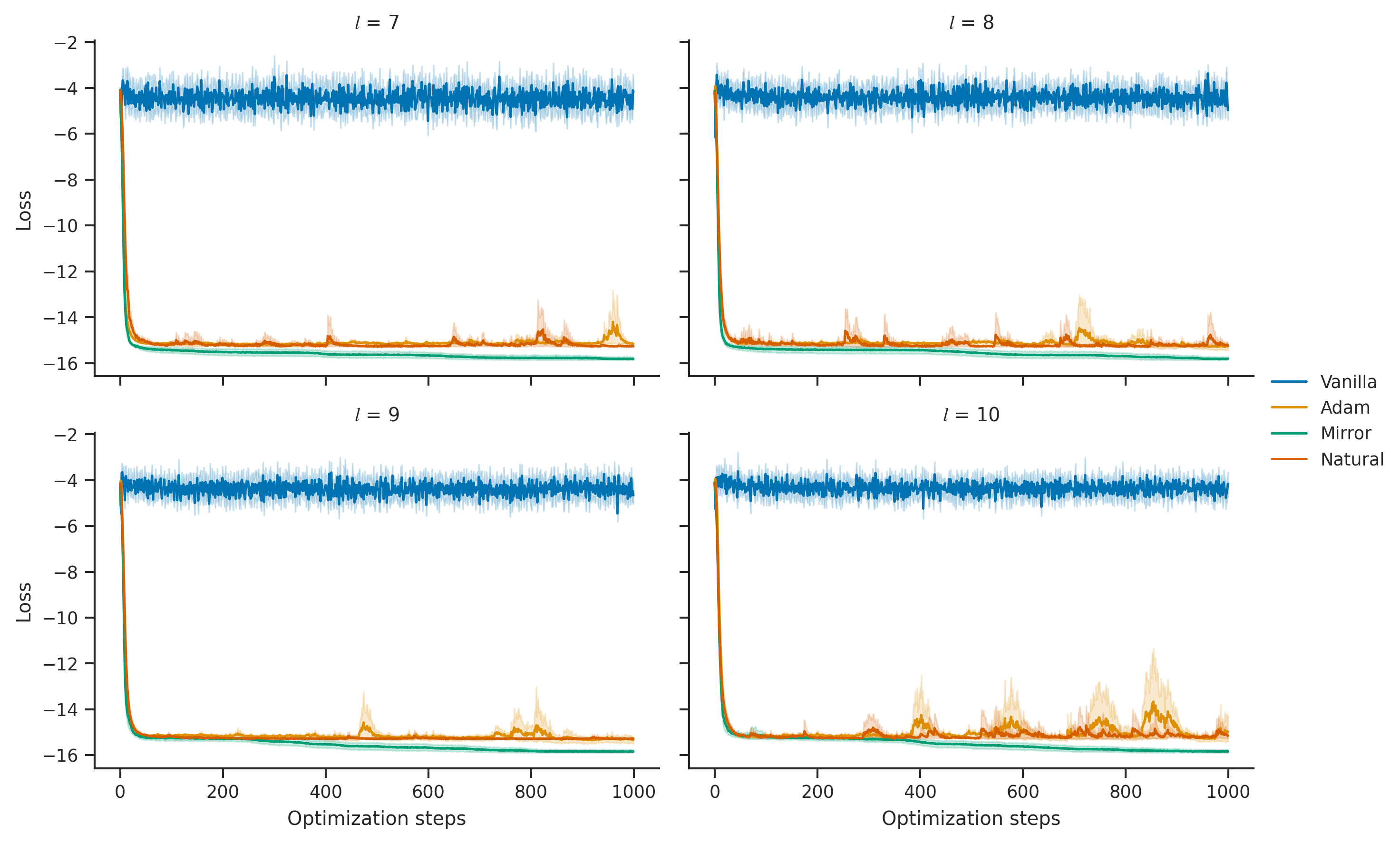

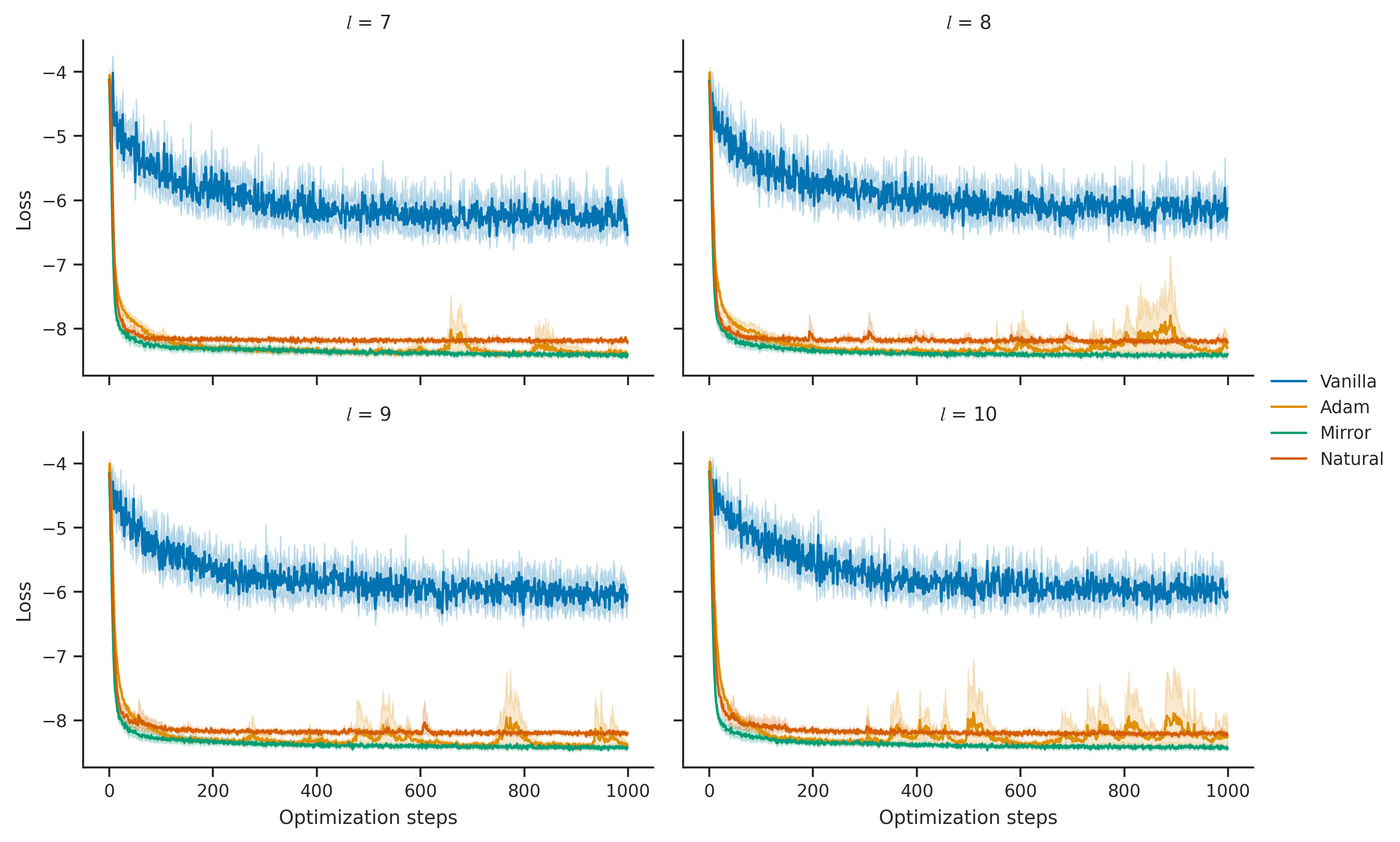


Appendix B Geometry of the space of quantum mixed states
In this section, we discuss aspects of information geometry needed for the design and analysis of Algorithms 1 and 2 in Appendices D and E. We begin with a background assumption.
Assumption B.1.
Our working Hilbert space is of dimension . The corresponding density operator space, , consists of non-singular4040 40 In this work, we will identity the Riemannian metric structure over with certain information matrices (as in eq. 27). However, it has been shown that this identification is possible so long as the rank of below does not depend on its classical parameterization [198, 199], since such information matrices otherwise become discontinuous. We will see that this positivity restriction asks that parameterize classical categorical distributions with full support over all bitstrings. density operators and . We write a variational density operator as4141 41 We note that this is simply the spectral decomposition, valid for any density operator: are eigenstates of with corresponding eigenvalues , and is just a labelling of those eigenstates. The separation of into distinct parameter sets and foreshadows our favored choice of ansatz; see Appendix G for more information.
| (19) |
where .
Now, in Section B.1 we discuss a theorem characterizing the set of Riemannian monotone metrics over . In Section B.2 we introduce two important examples of such metrics, which we will use frequently throughout this paper. We introduce several useful tools and terms in Section B.3. Then, in Section B.4, we will pull our example metrics back to a parameter space geometry over variational models of quantum mixed states. In the main text (Section III.3), we discussed how associating geometric structures to parameterized models can be beneficial for gradient-based optimization.
B.1 Characterizing monotone Riemannian metrics
We argued for the utility of monotone metrics in Section III. We restate the property formally below. From [99] we have the following definition:
Definition B.2 (Monotone Riemmanian metric over ).
A distance over is monotone if it does not grow under the action of a CPTP map (i.e., a quantum channel) ,
| (20) |
and if a monotone distance is geodesic then the corresponding metric is called monotone.
Monotonicity is a natural property to consider because it intuitively encodes the idea that, in general, stochastic maps are randomizing (i.e. coarse-graining should result in information loss) and so should draw distributions nearer to one another. Given the desirability of this property, in what follows we restrict our consideration to monotone metrics.
Which metrics are monotone? The classical (commutative) analogoue of a CPTP map is a stochastic matrix [99], and C̆encov’s theorem [109] says that, for categorical distributions, the Fisher-Rao metric is the unique metric (up to normalization) which satisfies classical monotonicity. In contrast, for the manifold of density operators , there are infinitely many monotone metrics [200]. In this quantum setting, the Morozova-C̆encov-Petz theorem [99, 201, 200] acts as the quantum generalization of C̆encov’s theorem. It characterizes the set of monotone metrics in terms of a mapping between (self-inversive and unital) operator monotone functions, , and monotone Riemannian metrics (see Section B.4 for examples). As a reminder, a metric defines an inner product taking arguments in the tangent space about . In particular, the tangent vectors on are traceless, Hermitian matrices (reminded in Proposition G.7).
Theorem B.3.
(Morozova-C̆encov-Petz) Let . Then, for any monotone metric , there exists a constant and function such that for any traceless Hermitian ,
| (21) |
Here, is symmetric and obeys . Furthermore, the function is operator monotone.
This theorem shows that there are many non-trivially different monotone metrics on the space of density operators. Note that, if we were to restrict consideration to the set of pure quantum states, we recover a natural uniqueness in the choice of metric. Thus existing works which consider metric-aware descent for pure state optimization have circumvented the question of choosing from among the various quantum monotone metrics [90].
We can also make the reverse implication of deriving a monotone metric given a function satisfying the criteria above. For that, we first make a definition:
Definition B.4.
A Morozova-C̆encov (MC) function is an operator monotone map satisfying and
It is not hard to show that Theorem B.3 yields a bijective correspondence between monotone metrics and MC functions; given a monotone metric , the function is MC. Conversely, if is MC, one defines , which by definition of MC functions, satisfies the properties of in Theorem B.3. Hence, inserting our into (21) (and fixing ) yields a monotone metric.
B.2 Examples of monotone Riemannian metrics
We pause the theoretical exposition to give two key examples of monotone metrics, defining them in terms of their corresponding MC functions.
B.2.1 Quantum Fisher Information (QFI) and the Bures-Helstrom (BH) metric
In the case of the BH metric, the MC function is given by
| (22) |
and so which is the reciprocal of the arithmetic mean. Amongst all operator monotone functions on which are self-inversive and unital, there exists a minimal and maximal function, i.e., MC functions that are everywhere smaller (resp. larger) than all MC functions [202]. The maximal function is in fact (22). It is the case that and so .
B.2.2 Quantum Relative Entropy and the Bogoliubov-Kubo-Mori (BKM) metric
In the case of the BKM metric,
| (23) |
and so and which together is the reciprocal of the logarithmic mean. It is the case that in mixture coordinates (Definition G.1) and so . Although is neither minimal nor maximal, we will use the facts that the implied metric is the Hessian of the canonical quantum relative entropy, (eq. 211), and a duality property (Section E.1) to motivate its usefulness. In exponential coordinates, the raising and lowering operators are swapped, a hint toward the duality property.
B.3 Tools for working with monotone metrics
We will apply several mathematical tools involving monotone metrics in Appendices D and E. We introduce some of these tools below.
B.3.1 Positivity of the metric
First, based on Theorem B.3, we have the fact that all monotone metrics over in our consideration are positive definite. For pedagogical purposes, we check this explicitly.
Proposition B.5 (Riemannian metric signature).
All monotone metrics over are positive definite under B.1.
We can then relate the positive definiteness of the metric to the positive definiteness of the metric resolved to a matrix in an arbitrary basis:
Corollary B.5.1.
Under B.1, any monotone metric over is positive definite when resolved to a matrix in terms of an arbitrary tangent space basis.
Proof.
Choosing a basis of traceless, Hermitian matrices, or frame, we can write the Riemannian metric tensor as a matrix,
| (25) |
so that arbitrary traceless, Hermitian matrices have value
| (26) |
and so is positive definite for all whenever is a positive definite Riemannian metric in that . ∎
B.3.2 Information matrix
It will be convenient to resolve the metric tensor to coordinates as a matrix. We will define the Information Matrix as having matrix elements
| (27) |
i.e. the pullback of the metric tensor to parameter space4242 42 Other definitions in the literature may include an inconsequential factor of 4, .. Here, denotes the choice of MC function which we saw to uniquely specify the metric at . We work the information matrix out in a particular ansatz class for the two metrics in consideration in Appendices H and I.
We note that is a traceless Hermitian matrix and so describes a tangent vector on at (Proposition G.7). This matrix is positive definite so long as gives a basis for the tangent space of at (Corollary B.5.1). It is possible to choose a model parameterization so as to either describe a smooth embedding or global diffeomorphism from to classical parameter space (Section G.2). However, this is not anticipated in general, particularly when strong inductive architectural biases are leveraged or consists of neural network parameters.
As we will see, in the -basis,
| (28) | ||||
| where, | ||||
| (29) | ||||
B.3.3 Raising and lowering the metric
We now describe another useful representation of the metric inner product. The choice of fixes a linear operator which acts as the metric with lowered indices. Hence, it allows us to write the metric inner product as the Hilbert-Schmidt inner product
| (30) |
for arbitrary tangent vectors . We can also define raising operators for the class of monotone metrics on :
Definition B.6.
The linear operator acts as the metric with raised indices and is defined so that, in the -basis [203],
| (31) |
and satisfies ,
| (32) |
Hence, for example,
| (33) | ||||
| (34) |
which matches the result of Theorem B.3 with and .
B.4 Monotone metrics over
Here we apply the metric raising and lowering operators to our two example metrics, BH and BKM. This lets us represent those metrics in model coordinates as generalized information matrices.
Example B.7 (Bures-Helstrom).
Choose as in (22) and so . Then, by (31), the linear operator writes
| (35) |
Hence, in the -basis, the lowering operator is given by
| (36) |
where . Therefore, the Quantum Fisher Information Matrix (QFIM) is given by
| (37) |
which we will resolve block-wise for diagonalized models in Appendix I.
Example B.8 (Bogoliubov-Kubo-Mori).
Choose
as in (23), meaning that
Hence, we say that where is the logarithmic mean. In this case, writes
| (38) |
Hence, in the -basis,
| (39) | ||||
| (40) |
Therefore, the BKM information matrix is given by
| (41) |
which we will resolve block-wise for diagonalized models in Appendix H.
Appendix C State discrimination bounds
In this section, we discuss the relationship between information geometry and metrology, leading to the concept of generalized QFI and the generalized QCRB. Significant literature [26] is dedicated to the fundamental metrological question of parameter estimation, especially in relation to the well-studied QCRB as it usually relates to the BH geometry. In the applications of quantum Hamiltonian learning and variational Gibbs sampling, we are essentially interested in estimating the parameters of an unknown quantum mixed state. We will discuss how searching for such parameters through a metric-aware gradient-based optimization can saturate fundamental asymptotic limits of parameter estimation (Theorem D.4) whereas this is not generally the case for other gradient-based strategies. In fact, other quantum natural gradient strategies have fallen short of such proven guarantees because of, intuitively, the discrepancy between the utilized curvature in state space and curvature of the objective [90].
The construction of a QCRB which generalizes beyond the BH geometry essentially involves a straightforward application of Cauchy-Schwarz for Hermitian operators. We provide the construction in Theorem C.1. In particular, take as a collection of quantum observables. Then, in the multi-parameter case, the generalized QCRB relates a covariance matrix at to the QFIM as,
| (42) |
where the generalized covariance is
| (43) |
and the bias matrix is
| (44) |
where is an arbitrary number of collected measurement samples of , and denotes the Moore-Penrose pseudo-inverse of a matrix . The linear operator is defined to satisfy .
Consider if we assume that is now a collection of quantum observables that are constructed as locally unbiased estimators to the optimal parameters . Note that is a locally unbiased estimator of at if
| (45) |
which holds if , the stronger condition of global unbiasedness. Clearly, in such a case, we have that . However, Corollary 7.7.10 of [204] taken with (42) implies that this can only be the case if the information matrix is non-singular. Therefore, locally unbiased estimators require that the parameterization gives a locally non-singular information matrix. So, in this case, we recover a simpler inequality,
| (46) |
Now, we can use the theory of MC functions to rewrite the covariance and information matrices. In the -basis [203],
| (47) |
with again as in (29).
Recall from Section B.2.1 that the MC function is maximal for the BH metric. Hence, for a single-parameter , the BH instance of Theorem C.1 gives the tightest guarantees with respect to the then scalar given that and . This is consistent with the fact that which verifies the claim for the two metrics we have detailed.
Finally, attaining the BH scaling (which is tightest for single-parameter), , is not always possible in the multi-parameter case. In proving the generalized bound, one implicitly assumes that each of the , the optimal parameter-estimating observables in , are informationally compatible. In other words, a necessary and sufficient condition to saturate the bound is that so that parameters can be estimated optimally independently of one another. It turns out that this condition holds for certain ansatzes as we show in Proposition C.3.
Following (43), we can write the generalized covariance between two observables as the inner product,
| (48) |
In such a case, it is useful to define an object termed the logarithmic derivative given by
| (49) |
which then induces the relation
| (50) |
We will use these relations to write a generalized QCRB, below.
Theorem C.1 (Generalized QCRB).
The generalized QCRB (42) holds.
Proof.
We generalize the proof from [203] to allow for a singular information matrix, as is anticipated for over-parameterized models like classical neural networks. Showing the inequality for a single sample is sufficient to verify the scaling.
For simplicity, we drop the metric specification, . Without loss of generality, we assume that and we will employ the block-matrix method. Hence, we may assume that we and write the estimators of (42) as and the logarithmic derivatives at as in (49) as . We write the inner product of (50) at plainly as .
We now state a necessary and sufficient condition for saturation of the QCRB under the BH choice of metric.
Lemma C.2 ([26]).
A necessary and sufficient condition for the saturation of the BH multi-parameter QCRB is
| (53) |
We’ll refer to the above as a compatibility condition for the logarithmic derivatives. Armed with this result, we can show that QHBMs (Appendix G) are parameterized in such a way that the tigtest QCRB can always be saturated.
Proposition C.3.
Let be coordinates for a QHBM . Then, the compatibility condition
holds. As a consequence, optimal parameter estimation for QHBMs, with QNNs amenable to parameter shifts, asymptotically saturates the Quantum multi-parameter Cramer-Rao bound.
Proof.
We break the proof into a few different cases. Let , so that , with and . Then, for all , we have
| (54) |
Henceforth, we write for notational convenience. A simple computation gives
| (55) | ||||
| (56) | ||||
| (57) | ||||
| (58) | ||||
| (59) |
where in the last line we used , which holds because the QHBM is diagonalized.
Now, we consider the condition for the parameters. We will see in (234) the form of the SLD,
| (60) |
For simplicity, denote and . Then, we have:
| (61) |
Splitting the above sum into two via the Kronecker deltas, then relabeling indices, yields the simple conclusion Our final task is to prove compatibility between the and parameters, i.e., that
We expand this assertion:
| (62) | ||||
| (63) | ||||
| (64) |
Importantly, we used Thus, the desired compatibility condition holds and we are done. ∎
Appendix D Metric-aware gradient descent
D.1 Derivation
In this subsection, we derive a general form for quantum metric-aware gradient descent where the monotone metric over parameter space geometry is left as a degree of freedom (see Appendix B). That is, we will derive that the metric-aware parameter update is the choice of parameter update which yields the steepest descent in towards the minimum of a loss function while maintaining a predetermined step size in .
The chosen monotone metric provides a notion of distance and length in parameter space which is a better representation of how changes in parameter space affect changes in state space. As such, evaluating this metric can be used to augment standard gradient descent strategies to obtain metric-aware gradient descent. Such a method can be considered a second-order method (as it uses second-order information about ). Although it can be more computationally costly per iteration, in many cases the descent procedure can converge on a significantly smaller number of iterations to the optimal parameters.
We can phrase our notion of steepest descent mathematically as the choice of () at gradient step following,
| (65) |
where is our loss functional and is a constant. Note that object of special interest is which describes a metric-related potential that is symmetric and bilinear up to third-order. In particular, we use the fact that every monotone metric is the Hessian of some potential [108],
| (66) |
where is the information matrix of the metric, as in Equation 27. Furthermore, the potential corresponds to a locally perturbed member of the family of so-called monotone relative entropies [108]. It is also the case that a monotone relative entropy obeys that is at a minimum of zero when implying that the first two orders of an expansion about vanish. An explicit computation then shows that (Corollary G.5.1):
| (67) |
Notice (8) is a constrained minimization problem, we can thus consider the relaxed Lagrangian,
| (68) |
We may expand both terms to their first non-vanishing order in and remove constants which do not depend on . The loss function will be expanded to first-order and the potential term to second-order,
| (69) | ||||
| Equivalently, | ||||
| (70) | ||||
| (71) | ||||
Differentiating (71) yields the metric-aware gradient update,
| (72) |
where will be our effective learning rate.
The objective (8) seems to indicate that the update rule is invariant under re-parameterization given its exclusive dependence on density operator arguments (assuming that is sufficiently small, so that the relevant approximations are sufficiently precise). This is indeed the case when the model parameterization describes a global diffeomorphism from (or a submanifold thereof) to classical parameter space4444 44 See Section E.3 for a relevant discussion.. However, the introduction of the pseudo-inverse breaks this invariance in general because, for example in the case where the model is over-parameterized, the pseudo-inverse re-introduces a coordinate dependence by outputting the solution to with minimum 2-norm. A common strategy to circumvent the pseudo-inverse is to regularize the information matrix choosing a sufficiently large . This has the interpretation of adding an independent Gaussian prior over parameter space as we will see from (259) and therefore likewise introduces a coordinate dependence.
D.2 Optimality guarantees
We now move to a setting of proving asymptotic optimality of the metric-aware gradient descent algorithm with the BKM metric. Hence, for simplicity, we will drop the qualifier throughout:
| (73) | ||||
| (74) | ||||
| (75) |
In particular, we will show that the BKM metric-aware update rule achieves the corresponding generalized QCRB in the limit of many steps. To this end, we provide the context for this result by first giving our assumptions.
Assumption D.1.
Assume that is a smooth immersion , hence defining smooth local coordinates on a submanifold of . Assume that the BKM metric-aware update rule
| (76) | ||||
| where, | ||||
| (77) | ||||
converges to the optimal parameters in expectation, i.e., as . Here, is an online unbiased estimator of the quantum relative entropy loss gradient obtained by the environment drawing a single pure state from the eigenstates of (with probability of the corresponding eigenvalue) at each optimization step4545 45 Any measurement on a target density operator can be viewed as a stochastic operation on its eigenstates..
The following proposition quantizes the formulation of [206] (see, in particular, eq. 48).
Proposition D.2.
Suppose the learning rate, for the update rule (76) taken in expectation,
| (78) |
is chosen as with initial parameters . Then, under the conditions of D.1, we have
| (79) |
asymptotically.
Proof.
We may Taylor expand the loss function as
| (80) | ||||
| (81) |
where we used that a generalized relative entropy and its gradient vanish at the optimum, and defined . As a consequence,
| (82) |
Similarly to (81), now expanding the first argument,
| (83) |
| (84) |
Equation 78 can be written
| (85) | ||||
| From (82), | ||||
| (86) | ||||
| From (84), | ||||
| (87) | ||||
| (88) | ||||
Within some neighborhood of the optimum, the approximations eqs. 81 and 83 are good enough so that 4646 46 This neighborhood may be arbitrarily small. See Remark D.3.. We have chosen . Therefore, neglecting the third order terms,
| (89) | ||||
| (90) |
for . ∎
Note that, for simplicity in notation, it is assumed that the learning algorithm begins at with initial parameters .
Remark D.3.
The convergence (79) is asymptotically which holds for any . We have used the fact that there exists some neighborhood of the optimum where . This neighborhood can be arbitrarily small, so long as it is reached in a finite number of steps, since we still use that convergence occurs as . This assumption is shared with Amari in his classical work [93], and so we follow this precedent. Providing a more practical non-asymptotic convergence rate generally requires specifying more information about the parameterized state or the target . Agnostic to this type of specification, we leverage Proposition D.2 to prove one of our main results, Theorem D.4. However, we will revisit this point in Section D.3.1.
The proof and theorem statement below should be contrasted with the classical analogue [110] which is proven with less machinery.
Theorem D.4.
Suppose D.1 holds. Then, the update rule (76) with learning rate induces a dynamical equation on any arbitrary initial choice of a collection of quantum observables, acting as estimators, such that the generalized QCRB (46) is attained asymptotically. The equivalent statement holds when one swaps arguments of the loss, .
Proof.
We will denote the th element of as . We will attempt to map the metric-aware update rule (76) in parameter space to a latent dynamical equation (induced by quantum expectation) in quantum observables. This will allow us to tie back to the parameter estimation language and bounds of Appendix C. So, let give the true value of , and assume that without loss of generality. Following (42), initialize a collection of quantum observables that satisfy , so that is an unbiased estimator of . In such a case, we can rewrite (76) in expectation (as in (78)) element-wise as
| (91) |
noting that this corresponds to the minimization of the reverse relative entropy loss. We have seen that . For the BKM, we can check from (208) that the first derivative satisfies,
| (92) |
Now, given (92),
| (93) |
With this in hand, we see that the metric-aware descent update (93) is the quantum expectation4747 47 As in D.1, the algorithmically relevant expectation can be estimated unbiasedly, for each , using a single pure state sample from the eigenstates of the data (sampled with probability of the corresponding eigenvalue). Of course, the tangent vector and information matrix require additional samples to estimate, but these depend only on the model. This is a quantum generalization of online learning. of latent dynamical equation
| (94) |
Hence, in expectation, (94) describes how our collection of quantum observables, acting as estimators, updates at each descent step. So, we seek to bound the associated error covariance matrix corresponding to the metric given element-wise by,
| (95) |
Using Proposition D.2 again, . Furthermore, using both sides of (94) and that and [203],
| (96) | ||||
| So, using eqs. 82 and 92, | ||||
| (97) | ||||
| (98) | ||||
| (99) | ||||
| Finally, applying Proposition D.2 once last time gives that | ||||
| (100) | ||||
| and so | ||||
| (101) | ||||
Therefore, asymptotically, assuming that converges to 4848 48 This scaling is reminiscent of the Bernstein-von Mises theorem [207].. Note that the same asymptotic result holds if we flip the argument of our loss function because quantum relative entropy is symmetric up to third-order (Proposition G.5). ∎
The meaning of an online gradient estimator for simulation is clarified in Section F.2.
D.3 Practical considerations of optimality guarantees
D.3.1 Non-asymptotic optimization
The result of Theorem D.4 is asymptotic (see Remark D.3). Hence, we may question the practical convergence properties (e.g. in mean and variance) when restricting to a small number of steps. We may do so from the lens of the expansions used in its derivation. From the proof of Proposition D.2, we saw that quantum Fisher efficiency depends on the iterates entering the locally quadratic convex region where
| (102) |
For this to be meaningful non-asymptotically, it is therefore important that the constant factor of the is sufficiently small. So, this condition is a useful diagnosis for a sufficiently well-behaved region, and is derivative of the conditions eqs. 81 and 83 which can be viewed as the primary approximations.
Hence, when considering learning a sequences of states, we recall that chained initialization (section VII.1) means initializing the parameters for each state (after the first) at the optimal parameters corresponding to the previous target state in the sequence. Therefore, we may consider how strongly the information matrix varies in parameter space as we travel along the sequence. This allows one to evaluate whether we (approximately) remain within the quadratic convex bowl as we step forward in the sequence of states initialized at the previous optimum. This depends on both the physical process described by the sequence and the specific model parameterization. To this end, we work out the relevant expressions specific to real-time evolution, imaginary time-evolution, and generalizations of the latter to any generic path in parametric mixed state space in Appendix L.
D.4 Another perspective into estimator moments
The following proposition allows one to approximate an arbitrary function of an online natural gradient estimator. Such a function may be any classical moment, for example.
Proposition D.5 ([208]).
Assume the update rule (76). The expectation of a smooth function at iteration is given by recursive equation
| (103) | ||||
| where, | ||||
| (104) | ||||
for sufficiently small .
Proof.
For simplicity in notation, write that . As in (76), the observation of data results in the model parameters update where .
We have said that follows the spectral distribution of which we write as . The conditional probability density obeys
| (105) |
in that describes the volume element such that example modifies the estimator from to a point in the rectangle . Hence,
| (106) | ||||
| (107) |
And so,
| (108) | ||||
| (109) | ||||
| (110) |
Hence, we may expand about and note that
| (111) | ||||
| (112) | ||||
| (113) |
Taking the expectation with respect to completes the proof. ∎
D.5 Sample-efficient learning of many-body states
The authors of [24] consider the particular exponential parameterization of target state with -local modular Hamiltonian having nonzero coefficients ; , over a finite-dimensional lattice so that
| (114) |
with as inverse-temperature. The interaction graph is assumed to be spatially local so that in terms of the number of qubits. The canonical representation is assumed so that are known non-identity Pauli operators. It is then shown that there are constants depending on the geometric properties of the lattice such that the Hessian of the log-partition function (aka free energy) satisfies
| (115) |
Now, Theorem D.4 implies that, for quantum metric-aware descent in the parameterization,
| (116) |
where we may write the induced with that . In mixture coordinates, we have that where as in (130).
Lemma D.6 ([123]).
The which achieves the BKM QCRB scaling i.e. asymptotically is given by
| (117) |
Proof.
We verify this explicitly.
| (118) | ||||
| (119) | ||||
| (120) |
which verifies that achieves the QCRB scaling because the metric tensor in mixture coordinates is inverse to the one in exponential coordinates given that mixture coordinates can be seen as covariant with exponential as contravariant
From Lemma D.6, we may consider this choice of to be the efficient estimator from the perspective of the BKM geometry. We note that and (195) shows that .
We will see in (128) that the BKM information matrix is equivalent to the Hessian of the log-partition function in the exponential coordinates. In their work and subsequent works [25], the connection with information geometry and parameter estimation bounds (e.g. Fisher efficiency) is not identified. This is reasonable because their observable estimators (measurements are taken to be the ) do not match the ones (117) which we termed the efficient estimators in the eyes of the BKM, in general. However, clearly, in our case this identification is appropriate because quantum Fisher efficiency ties this quantity as a metric to our algorithm’s convergence rate; this identification allows a straightforward sample-efficiency upper bound argument when paired with a strong convexity bound on the free energy.
With this in mind, we have that
| (121) | ||||
| (122) |
It remains to show how relates to expected variations in the estimator . To achieve this, we will consider a large deviations perspective [211]. Large deviations analysis characterizes the exponential rate of convergence in the probability of the estimated parameters being greater than some constant.
Lemma D.7.
Define to be the estimator of found by a finite averaging of outcomes from the observables . Suppose that converges asymptotically and satisfies quantum Fisher efficiency (122). Then, there exists a sufficiently small neighborhood about such that
| (123) |
Theorem D.8.
With probability , the algorithm (77) learns the target Hamiltonian to error with using
| (124) |
data samples, asymptotically.
Proof.
First, Equations 37 and 41 gives that
| (125) |
Hence, combining Lemma D.7 and (122) gives that the failure probability is met after
| (126) |
descent steps asymptotically. Since we want all estimates to fail with probability less than , it suffices to set and apply the union bound. Finally, each descent step, if implemented as (77), requires samples from the quantum data. ∎
This samples scaling is a factor of greater than the optimal in [25] and so looser than the one found for the (differing) marginals matching strategy of [24] by a factor of . Our scaling does not involve a restriction on . Note, however, that in the high-temperature regime it was shown that (115) can be improved to eliminate the dependence on [25].
Note that it is understood that achieving a stronger version of (123) so that the RHS is given by requires so-called super-efficient estimation [212]. In particular, as a necessary condition, one must be able to measure multiple Gibbs states collectively i.e. leveraging quantum correlations between several states and a single measurement apparatus. We observe that the theoretically optimal samples scaling for the -norm, for general , may then be provable in such a scenario using similar techniques as above.
Appendix E Mirror descent equivalence
In this section, we show that performing Natural Gradient Descent using the BKM metric in the exponential family coordinate representation is equivalent to performing so-called Mirror Descent in the mixture family representation. This means that, under a particular Legendre transform, we can translate the proposed second-order method on our primal manifold to a first-order method on the dual manifold. In fact, under the BKM metric, the primal and dual manifolds are equivalent [123]. Hence, we can interpret this strategy as a special change of coordinates for which differing Riemannian connections vanish (i.e. they are flat in differing senses). We will then interpret the implication in the context of other model parameterizations in Section E.3.
Translating from a second-order to first-order method may be computationally beneficial (less parameter-shifted observables). Furthermore, compared to the method of minimizing over the non-truncated Lagrangian directly by gradient descent (V.2), this decouples the loss function from the inner loop.
E.1 Convex duality
The first part of our description follows a known result that the BKM metric is the unique monotone metric for which the mixture and exponential flat affine connections are mutually dual [123, 124] (and so the Levi-Civita connection is the average of the two, tying these connections to the metric tensor [110]). We review in Section F.1 the mixture coordinate decomposition of in a basis identifiable with : where are traceless, Hermitian matrices and . Similarly, we will recall the exponential coordinate decomposition of the modular Hamiltonian as . We now work within these two parameterizations and translate our results to arbitrary coordinate re-parameterizations in Section E.3.
The (dual) Riemannian metric tensors for the mixture and exponential global coordinate charts can be expressed as the Hessians of dual convex potential functions, which are related by Legendre transform. This fact is guaranteed by the aforementioned dual flatness [213]. The Legendre transform is a frequented device in thermodynamics and other physical study, for example describing the relationship between temperature and entropy as conjugate quantities. In this sense, we can think of , above, as inverse generalized temperature coordinates and , below, as entropy coordinates.
Conversely, dual coordinates are guaranteed to exist when the metric can be given in terms of a scalar function termed the potential function (this is in fact a necessary condition). In our consideration, we have this existence when we consider the BKM metric and take the log-partition function (aka free energy) to be the potential, , by observing that,
| (127) | ||||
| (128) |
which matches the result of (203) since
Definition E.1 (Legendre transform).
The Legendre transform of is the function defined by
| (129) | ||||
| implying that | ||||
| (130) | ||||
Hence, from (127), . Of course, the above also implies that the metric tensor in can be given by .
E.2 Mirror descent
Lemma E.2 (Theorem 2 of [214]).
Define,
| (131) |
to be the quantum Shannon entropy, , before tracing and with a sign flip. Then, the quantum Bregman divergence in is equivalent to the quantum relative entropy,
| (132) |
where
| (133) |
Observe that the Bregman divergence in is simply the first-order expansion of around evaluated at .
Proposition E.3.
Using mixture coordinates , define,
| (134) |
Then, the quantum Bregman divergence in is equivalent to the quantum relative entropy,
| (135) |
where
| (136) |
Proof.
Of course,
| (137) |
For this particular choice of coordinates, is linear in . Hence,
| (138) | ||||
| (139) | ||||
| (140) |
Therefore, we may directly apply Lemma E.2. ∎
Lemma E.4 (Dual potential).
Proof.
Hence, the metric tensor in can be given by .
Theorem E.5 (Dual relationship between mirror descent and metric-aware descent, non-commutative case).
The mirror descent update rule in mixture coordinates ,
| (146) | ||||
| is equivalent to the Natural Gradient update rule in exponential coordinates , | ||||
| (147) | ||||
Proof.
Recall that . Taking (146) with Proposition E.3 and differentiating in mixture coordinates gives,
| (148) | ||||
| Hence, from (136), | ||||
| (149) | ||||
| By Lemma E.4 and Definition E.1, | ||||
| (150) | ||||
| since implies that | ||||
| (151) | ||||
where the loss reparameterization . ∎
A duality between mirror and natural gradient descent has been explored in the classical literature [68] and so we have demonstrated a non-commutative analogue which required a specific choice of monotone metric. A parallel argument can be checked to hold if we were to begin with exponential coordinates and derive a natural gradient update rule in mixture coordinates. It is practically important to recall that exponential coordinates are unconstrained over the reals, whereas mixture coordinates are constrained.
Finally, note that in some cases the forward relative entropy may be computationally preferred to the reverse. In this light, it is worth noting that they are equivalent up to second order in the perturbation, (Proposition G.5). Hence, we may consider the approximation, .
E.3 Translating to general ansatzes
The result Theorem E.5 is shown for a special choice of global coordinate charts, and we may seek to interpret the result for some other choice of coordinates. Relatedly, we have indicated in Section D.1 that metric-aware descent (QPNGD) is invariant under smooth, bijective re-parameterization in the limit of an infinitesimal learning rate, which we will now check explicitly. Assume exponential coordinates , or any other global coordinate chart. Let us write this explicitly for (69), viewing dynamically and writing since iterations are taken to be infinitesimal ,
| (152) |
When we specify the boundary condition , the evolved path has been referred to as the Riemannian Gradient Flow [125], which we will see offers a coordinate-independent perspective into the relationship between metric-aware and mirror descent. Viewing (152) as the primary object, we see that the metric-aware descent update is a forward Euler discretization with the learning rate as the stepsize.
Let us consider what happens to the dynamics of (152) when we perform a change of coordinate chart, for example from exponential coordinates to projected QHBM coordinates4949 49 See Section G.2.3. . Let be the diffeomorphism that changes coordinates from exponential to another parameterization. Then, let designate the Jacobian matrix . Hence, by the tensor transformation law (equivalently, thinking about how the second fundamental form transforms),
| (153) |
recalling that . Therefore,
| (154) | ||||
| (155) |
which describes same flow. We check this explicitly by verifying that is a solution to (152) whenever is a solution. Indeed,
| (156) | ||||
| (157) | ||||
| (158) |
Therefore, we have verified that the flow (152) is invariant under re-parameterization, also termed intrinsic in the sense that it is intrinsic to the manifold. As another interpretation, recall that (155) is precisely the definition of the equivalence relation that defines the tangent space of a manifold when written in coordinates. Combined with (152), this observation implies that for all , hence meaning that (152) is a well-defined differential equation on .
We can view mirror descent as an alternative discretization of this flow when working in the BKM geometry, similar to as we have commented for metric-aware descent. Explicitly, we have said that metric-aware descent (QPNGD) is a forward Euler discretization of (152) meaning that it is evidently the linear interpolation of
| (159) |
where and . Consider if we instead were to only discretize the gradient, working now in mixture coordinates ,
| (160) |
We will check that this identifies with the mirror descent update (146) as considered in [125]. So, consider the mirror descent update (149),
| (161) |
From this relation, we can construct a path by linear interpolation, ,
| (162) |
so that at the interpolation points. Hence, we see that is smooth between these points, obeying . In such a case, the chain rule implies that
| (163) | ||||
| (164) |
which matches (160). Since we have only discretized the gradient, mirror descent (QPMD) can be considered a ”more accurate” discretization of (152), being more faithful to the geometry of the search space. This has been commented classically [125].
Now, let us consider a solution to (160) and transform coordinates by smooth, bijective . As in (157),
| (165) | ||||
| except now | ||||
| (166) | ||||
and so the discretized flow is not invariant under re-parameterization i.e. it is extrinsic in general. This is true except when which would mean that is constant meaning that the coordinates are affinely related. A similar argument holds for the metric-aware descent discretization.
So, for arbitrary coordinate charts of in the BKM geometry, metric-aware descent (QPNGD) and mirror descent (QPMD) are generally distinct and extrinsic discretizations of an intrinsic flow; however, they are equivalent discretizations for special parameterizations related by Legendre transform as in Theorem E.5.
Appendix F Quantum exponential and mixture family ansatzes
F.1 Mixture and exponential coordinates
In the literature [123], mixture or Bloch coordinates may refer to the decomposition of in a basis identifiable with . In particular,
| (167) |
where are traceless, Hermitian matrices and . The positivity of density matrices implies that the Bloch coordinates must be constrained; e.g., when , .
Similarly, exponential coordinates may elsewhere refer to the -identifiable decomposition of the modular Hamiltonian as
| (168) |
with unconstrained.
F.2 Online loss gradients for exponential family
We check here that the gradients of the loss for the mixed state ansatz [80] (quantum exponential family, as above) which we used in Section D.5
| (169) |
where are known non-identity Pauli operators, can be estimated using a single data sample (for learning) or Gibbs state preparation (for simulation). The motivation is so as to implement online natural gradient descent (76). A similar calculation is feasible for QHBMs (Appendix G).
For the reverse relative entropy loss (188),
| (170) | ||||
| (171) |
where is the eigenvalue distribution over the eigenstates of . Hence, a single sample from the data distribution is sufficient to have an unbiased estimator of the above gradient which is the resource we count in determining quantum Fisher efficiency. Nevertheless, in general, many samples from the model distribution are required to estimate the quantum log-partition function gradient [215], which involves complications due to the non-commutativity between the thermal state and its gradient [80]. A key motivation for the QHBM ansatz is to translate this sampling problem (via (QPRGF)) – while NP-hard to compute exactly – to be classical by utilizing the spectral representation of density operators. In this way, the classical log-partition function gradient can be computed offline from the quantum computer, and diagonalization eliminates quantum-specific complications like the sign problem. Quantum algorithms which diagonalize density operators (thus splitting the quantum sampling problem into a classical sampling problem followed by a unitary transformation) are expected to be efficient in broad cases where classical sampling from the quantum thermal distribution is not [83] (for example, under the ETH assumption [87]).
Similarly, for the forward relative entropy loss (183) where we seek to simulate given its modular Hamiltonian,
| (172) | ||||
| (173) | ||||
| since is traceless and so , | ||||
| (174) | ||||
where is the data distribution as before. Hence, for the problem of simulation, the resource counted by Fisher efficiency is only the number of measurements of the known Hamiltonian against the variational Gibbs state.
Appendix G Review of Quantum Hamiltonian-Based Models (QHBMs)
We refer the reader to Verdon et. al [86] for a comprehensive description of QHBMs. However, for completeness, we review the essential details to our work here. Now, generally, QHBMs are variational circuits intended to learn descriptions of mixed quantum systems. We can view these circuits under two equivalent representations, as subsequently defined.
Definition G.1 (“Mixture representation”).
One may parameterize an arbitrary density operator as,
| (175) |
in terms of classical parameters which specify the classical probability distribution with and the unitary QNN [2] .
Definition G.2 (“Exponential representation”).
Equivalently, one may parameterize an arbitrary density operator as
| (176) | ||||
| with the so-called modular Hamiltonian, | ||||
| (177) | ||||
| and its partition function, | ||||
| (178) | ||||
where is referred to as the real-valued “energy” function.
Note that our notions of exponential and mixture representations differ from similar terminology in the quantum thermodynamics literature [123], though we adopt this naming due to a straightforward identification of the respective representations. In particular, referring to Section F.1, for mixture coordinates there exists a bijection between and (with describing the projected coordinates of (199)). And, notably, the important structure of being constrained over the reals is shared. For exponential coordinates, there is a bijection between and . Likewise, is unconstrained over the reals.
Evidently, and are related in this case by,
| (179) |
and, in the classical statistical learning literature, a statistical model specified in coordinates is termed an EBM [216, 217] and so the apt naming of Quantum Hamiltonian-Based Models (QHBMs). The EBM serves as the main vehicle to add classical correlations in the QHBM representation, while the QNN serves to add multipartite quantum entanglement, the latter of which cannot be captured at scale by classical models [168], or sampled efficiently from using classical computers in general [19].
Optimizing graphical models in terms of directly (which may, for example, be a neural network) is a popular choice because one effectively relaxes the constrained optimization problem in to be unconstrained. One must however cope with the fact that estimating (required e.g. for gradient updates in ) may be computationally intractable when is sufficiently large. So, Markov-Chain Monte Carlo (MCMC) approximation algorithms are customarily classically invoked [218, 219, 220, 221]. One may proceed similarly in the quantum case (see the discussion in [86]); preferred MCMC algorithms may leverage the discreteness or possible differentiability of for improved sample efficiency.
From the spectral decomposition theorem of Hermitian operators, for a sufficiently expressive energy function and QNN, this hypothesis class can cover the whole space of density matrices, as the QNN acts as a diagonalizing unitary. In our applications, we aim to have parameterizations for both the EBM and the QNN which possess an inductive bias for better trainability through metric-aware optimization, which will yield improved optimization behavior.
G.1 Quantum Relative Entropy
The QHBM training loss function motivated in [86] is the quantum relative entropy defined as [107]
| (180) | ||||
| (181) |
in terms of the von Neumann entropy and with . Evidently, with equality if and only if .
The quantum relative entropy is a non-commutative generalization [222] of the Kullback-Leibler divergence [223] which is a conventional loss function in classical probabilistic machine learning [224]. Observe that the quantum relative entropy is asymmetric in its arguments as in the classical case. The two applications briefly described next highlight this asymmetry.
G.1.1 Applications
One may learn an unknown mixed state in the QHBM parameterization through gradient-based optimization in either the forward or reverse quantum relative entropies: and , respectively. As the true modular Hamiltonian of the data distribution is unknown, we usually minimize alternate but equivalent losses, being that of quantum cross-entropy and quantum free energy, respectively. The algorithms to do so via gradient-based optimizers or otherwise are called Quantum Modular Hamiltonian Learning (QMHL) and VQT, respectively [86].
The preferred choice in terms of tractability depends on what is known a priori, for example in simulation as compared to characterization scenarios. Gradients can be computed through special stochastic averages of parameter-shift rules [225]. For notational convenience in some instances we might denote the quantum relative entropy between two QHBMs as
Variational Quantum Thermalization (VQT)
Suppose the provided input is a Hamiltonian and an inverse temperature . An important task using this information is to simulate the associated thermal state,
| (182) |
a task also known as quantum Gibbs sampling. Gradient-based optimization of this task is feasible using QHBMs. See the discussion at section VI for more on quantum Gibbs sampling.
Summarizing a result of [86], using Equation 180 and the QHBM ansatz of Equation 176, we may minimize the forward quantum relative entropy and so implicitly define the VQT loss.
Definition G.3 (VQT loss).
The VQT loss is given by,
| (183) | ||||
| (184) | ||||
| (185) |
In the following we assume the EBM parameters and QNN parameters are distinct. Then the derivative of the VQT loss with respect to the classical model parameters is
| (186) |
where we defined the push-forwards Hamiltonian and the push-forwards Hamiltonian expectation per basis state .
Similarly, the gradient of the VQT loss with respect to the quantum model parameters is
| (187) |
Quantum Modular Hamiltonian Learning (QMHL)
Dual to the task of VQT, suppose we are given query access to prepared thermal state and seek to fit a parameterized modular Hamiltonian (as in (177)) such that the corresponding model state is as close as possible to . This is a modified version of the Hamiltonian learning task defined in section (II.1). To derive the QMHL loss, consider taking the relative entropy in the reverse order as compared to VQT:
Definition G.4 (QMHL loss).
The QMHL loss is given by,
| (188) | ||||
| (189) | ||||
| (190) |
The gradient of the QMHL loss with respect to the classical model parameters is
| (191) |
where . Using our notation for the pulled-back data state , the gradient with respect to unitary QNN parameters will be given by
| (192) |
G.1.2 Additional properties
While the quantum relative entropy is asymmetric (as is the classical KL-divergence), it is nearly symmetric for nearby states, as we show in the following result. Proposition G.5 is standard and well-known [226], but we give our own explicit proof, as it will be useful in other parts of this work.
Proposition G.5.
The relative entropy is symmetric up to third order. That is, for any (sufficiently smooth) parametrized density operator , we have
| (193) |
Proof.
We know that:
where we used that . Now, a simple computation involving the definition of the relative entropy (eq. 208) gives:
| (194) |
Let , so that . Then, we see from the infinitesimal form of the Baker-Campbell-Hausdorff formula – and some algebraic manipulation – that
where we’ve suppressed explicit dependence in the last line for brevity. Substituting the above into (194) and using the linearity of trace, we find
where we used that , that , and finally the simple identity, . Hence, combining the above with (194), we conclude that
| (195) |
Now, we consider the second order terms,
But now, we observe that
Hence, combining the above calculations, we conclude that
Similarly, we obtain readily that
which immediately implies that and agree up to third order terms, i.e.,
as desired. ∎
Corollary G.5.1.
The above line of reasoning immediately yields the following equivalent forms of the BKM metric:
| (196) |
where the starting definition (204) stems from a more general scope of dual metrics [227].
Proof.
Recall from the proof of Proposition G.5 that for any smooth parameterized density operator , we have
Now, for any , we can fix the other coordinates and view as a 1-dimensional family of density operators, which immediately gives
| (197) |
Note that (197) holds for any parameterization . Now, differentiating (197) with respect to and applying the chain rule yields
which is exactly the the equality in (196). ∎
G.2 On the over-parameterization of QHBMs
In the QHBM (spectral) parameterization (Definition G.1), in general, parameterizes an arbitrary categorical distribution (with full support as per B.1) in and . Similarly, in the absence of an inductive bias, parameterizes an arbitrary element of and . Hence, there exists a straightforward projection map which acts independently on the classical and quantum parameters of .
In such a case, the parameterization map which acts as cannot be injective given that . So, to construct a manifold chart [110] of we must project out dimensions from the image of . We describe a mechanism to do so in this section. Such a construction relies on the generalized Euler angle parameterization [228] and the fact that diagonal density operators commute with diagonal unitaries which leads to a characterization of the invariant actions.
With and , we say that,
| (198) |
We note that acts only on the quantum parameters; hence, even with projection, the quantum and classical parameters of a QHBM are decoupled from one another.
So, we have counted above that the classical parameters which encode a can be thought of as and after an implicit projection. We also know that the real dimension of is . Hence, it appears at first glance that QHBMs are over-parameterized. This indicates that cannot chart the Riemannian manifold directly. Hence, we identify a (conveniently, global) projection map so that its image gives appropriate (global) coordinates. Accordingly, we project out a dimensionality of through a map which acts precisely on the parameters,
| (199) |
G.2.1 Isotropy of under action of
A means to resolve the over-parameterization5050 50 Our discussion follows the one of [99] regarding the “stratification” of into orbits of the unitary group. is to observe that the diagonal commutes with certain unitary and therefore is invariant under the conjugation . And note, all such may be classified as the Cartan subgroup [229] of acting on ; the Cartan subgroup is an exponential of a set of simultaneously diagonalizable elements of the algebra and so holds dimension . We resolve the details for the full-rank, non-degenerate special case next.
Consider a non-degenerate and full-rank transformed to its diagonal frame with image . Evidently, is invariant under precisely the conjugate action of an arbitrary diagonal unitary . In this sense, and so is determined up to the arbitrary phases entering . Hence, we can identify the isotropy group at hand with the -dimensional set of diagonal, unitary matrices. And in particular, we can identify this group with the of factors (denoted and thought of topologically as independent 1-tori).
Note that the isotropy group becomes more interesting when, for example, has degenerate eigenvalues.
G.2.2 Flag manifolds
In Section G.2.1, we have effectively described as the flag manifold which describes the space of all flags by identifying as an isotropy group of acting on . In our case, a flag consists of sequences of subspaces that reside in .
G.2.3 A suitable projection map
Consider a generalized Euler angle parameterization [228] of . In light of Section G.2.1, we can construct such a parameterization so that the isotropy group projects out. We refer the reader to [228] for details in that our described algorithms ultimately utilize the unprojected QHBM parameterization. However, we note and exemplify the essential points relevant whenever a manifold chart is required in our analysis.
In constructing a generalized Euler angle parameterization of , one uses the so-called Cartan decomposition (a generalization of the singular value decomposition to a semisimple Lie group or Lie algebra) to decompose into the semi-direct sum of two subspaces . It can be shown that are orthogonal complements of each other with respect to the Killing form on (i.e. and so under the Hilbert-Schmidt inner product). Any subalgebra of is commutative and in particular contains the diagonal elements of . In the generalize Euler angle parameterization, such elements act rightmost in the decomposition and so whose corresponding exponentials can be dropped. The following example demonstrates this for .
Example G.6 ().
Consider that we may write an arbitrary unitary when as,
| (200) |
and observe that the term can be dropped since is diagonal and so always commutes with .
Proposition G.7.
The tangent vectors of in the QHBM and projected (Section G.2.3) QHBM parameterizations span the set of traceless, Hermitian matrices. The unprojected QHBM parameterization tangent basis is over-complete by a dimension of .
Proof.
Let . We can rewrite an arbitrary density operator in the affine (Bloch) parameterization (see Section F.1),
| (201) |
where are traceless, Hermitian matrices i.e. Hermitian generators of . Hence,
| (202) |
and is closed by definition of being an algebra5151 51 Another way to see the tracelessness is that .. From (202), we see that the projected QHBM parameterization admits tangent vectors which span so long as the vectors
are linearly independent. Since charts , these coordinates are locally diffeomorphic to . The differential of a diffeomorphism is injective and therefore surjective, and so we have the desired spanning property. Since the unprojected QHBM parameterization includes redundant degrees of freedom, the same holds although its tangent vectors specify an over-complete basis. ∎
Appendix H Estimating the BKM metric tensor
We will now cover how to obtain the BKM metric tensor of the parameters in terms of the QHBM parameterization. In particular, we provide analytical expressions for sampling-based techniques to obtain unbiased estimates of the information matrix elements. We split up our information matrix calculation into three types of blocks of this matrix; the cases where the tangent vectors are both of parameters, the cases where they are both parameters, and the cases where they are a mixture of both types of parameters. The fact that we can compute analytic expressions for the metric tensor for which we can sample the values using a mixture of the quantum and classical computers is unique to the QHBM class of models.
In particular, when resolving the metric to a basis we may use that of the tangent vectors so as to assume the parameter space dynamics induced by the QHBM parameterization [230],
| (203) | ||||
| (204) |
using eqs. 27 and 40. We have also used the following identity, which will be very helpful throughout the course of this work:
| (205) |
Note as well that
| (206) | ||||
| (207) |
using Proposition G.7. We have termed (203) the BKM information matrix. We now discuss its relationship to the relative entropy; recall that the quantum relative entropy can be written in the following form:
| (208) |
In Section B.2.2, we claimed that the BKM inner product is related to the Hessian of the relative entropy. To establish this claim, write:
| (209) |
Evaluating the above at , we find:
| (210) |
Therefore,
| (211) |
We will use (204) in what follows. Recall from Section B.2.2 that our choice of lowering and raising operators implies we are working in mixture coordinates (Definition G.1) meaning that the partition function is parameterized directly by . The metric tensor resolves equivalently in exponential coordinates, where the raising and lowering operators are exchanged. In exponential coordinates, tangent vectors enter as .
H.1 EBM block
We first compute the BKM logarithmic derivative,
| (212) | ||||
| (213) |
and tangent vector,
| (214) | ||||
| (215) | ||||
| (216) | ||||
| (217) |
Critically, given that the eigenbasis of is independent of . Therefore,
| (218) | ||||
| (219) | ||||
| (220) |
The result reads as the covariance matrix of the gradient vector of the energy function subject to the sampled EBM distribution. Note that this quantity does not require a quantum computer to be evaluated.
H.2 QNN block
For the BKM metric tensor elements which only depend on the gradients with respect to QNN parameters, we can use an intuitive double parameter shift rule. A gradient technique for unitary QNNs was recently pointed out in [231]; here we can apply it to the gradients of the QHBM QNN parameters. For a hardware efficient ansatz (i.e. a QNN whose parameterized operations are independently parameterized and are of the form of simple exponentials of single Pauli operators, , e.g. ), we have the parameter shift rules,
| (221) | ||||
| (222) | ||||
| (223) |
with where standard basis vector has entries .
H.3 Coupled block
Appendix I Estimating the BH metric tensor
I.1 EBM block
We can find the same EBM block result as (220) in terms of the QFI which corresponds to the BH metric. As we will see from (49), the defining relation of the Symmetric Logarithmic Derivative (SLD) is given by
| (225) |
Equation 225 can be viewed as a special case of the Lyapunov equation which admits solution . Since ,
| (226) | ||||
| noting that, | ||||
| (228) | ||||
Furthermore, noting (50) and using eqs. 217 and 228,
| (229) | ||||
| (230) | ||||
| (231) | ||||
| (232) |
as expected, classically.
I.2 QNN block
We now proceed similarly for ,
| (233) | ||||
| referring to (222). Taking matrix elements in the -basis with , | ||||
| (234) | ||||
| Hence, | ||||
| (235) | ||||
which matches (28). In this (non-commutative) case, we see that the result does not match the BKM metric result of Section H.2.
I.3 Coupled block
Appendix J Metric-aware optimization of sequences of tasks
It is useful to classify sequence models as either recurrent or regressive. In the case of a recurrent (or recursive) task, the sequence is specified in terms of a quantum map which links each modeled density operator to the next one in the sequence. On the other hand, in a regression task, query access to the entire sequence of states is supplied directly. For our numerics, we focused on sequential conditional optimization (Algorithm 3), and recursive conditional optimization for QVARTZ.
J.1 Quantum-stochastic processes description of quantum dynamics
First, let us review the general mathematical theory of quantum open system dynamics [232]. We can define a superoperator which takes a density operator as argument and outputs a different density operator in the same space of operators, . The output density matrix is then denoted as . One general form of this operator is the Liouvillian superoperator written as
| (239) | ||||
| where, | ||||
| (240) | ||||
such that the Hamiltonian is a Hermitian operator, are termed the jump operators (both of these can generally be time-dependent), and is a general superoperator known as the quantum memory kernel. The standard Liouville-Von-Neumann equation describes a closed quantum system and is the special case where the latter two terms on the RHS vanish.
The solution to Equation 239 can then be expressed as a superoperator-valued time-ordered exponential of the Liouvillian,
| (241) |
where the effective channel superoperator which takes the state at time and outputs the state at time is called the propagator.
The differential equation describing the time evolution of an open quantum system under the Born-Markov [233] approximation assumes that the memory-carrying term of Equation 239 vanishes,
| (242) |
In such a case, we may refer to the Liouvillian as a Lindblad superoperator. For the scope of this paper, we consider how to learn quantum states coming from Markovian time evolutions where the above approximation holds, though all of our described techniques should generalize to non-Markovian sequences of completely-positive trace-preserving maps.
J.2 Generic Sequential Optimization for Sequences of Tasks
Suppose we have a sequence of target states given by a partition of a discretized parametric path in task parameter space . We wish to learn a sequence of optimal QHBM parameters so that each for each . Hence, we can have a collection of loss functions
| (243) |
For sequential optimization, we can apply Algorithm 3 to the above sequence of losses in order to find these optimal parameters. We then obtain a full approximation of the quantum-stochastic process [164] formed by the sequence of states along the chosen task path,
| (244) |
This is the approach for both Meta-VQT (Section J.3) and QSPL (Section J.4). At an abstract level, the principle difference between both these algorithms is that for Meta-VQT, we minimize sequentially the forwards quantum relative entropy between model and target state; , while in QSPL, we minimize the backwards quantum relative entropy between model and target state; . Let us flesh out below how the physical contexts of the target datasets differ.
J.3 Meta-Variational Quantum Thermalization (Meta-VQT)
Consider the case where we are given a sequence in the space of target modular Hamiltonians rather than the states themselves. Then our sequence of target states is a sequence of thermal (Gibbs) states
| (245) |
where is a path function in the task parameterization space of dimension . Note that, this path parameter vector can include both coldness (inverse temperature; ) and Hamiltonian parameters.
In order to find sequence of optimal QHBM parameters such that the relative entropy between our models and the target states are minimized throughout the sequence, we minimize each of the free energies:
| (246) |
and where we denote the free energy of the state with respect to the Hamiltonian , also known as the VQT loss,
| (247) |
Results from Section VII.1 came from choosing this VQT free energy loss for as in (243) and Algorithm 3. Note that the gradients of this loss can be straightforwardly estimated, see (183) for the explicit gradient estimators. We term this Gibbs-sequence-generating problem Meta-Variational Quantum Thermalization (Meta-VQT),5252 52 One can understand this choice of name as akin to a Meta-learned VQT optimization algorithm. and we can apply our chained metric-aware optimizer (Algorithm 3) to sequentially optimize these free energy losses. In our results section, we mainly focused on chained QPMD.
A special case of Meta-VQT is for imaginary time evolution, where the path in coldness-Hamiltonian space is variable only in coldness (inverse temperature); . In this case of application of Meta-VQT to imaginary time evolution, the Meta- prefix can also be understood to stand for Multi-Euclidean-Time-Annealing. This imaginary time evolution special case is what we focus on for the results of Section VII.1.
J.4 Quantum-Stochastic Process Learning (QSPL)
For Quantum-Stochastic Process Learning (QSPL), the task is to generatively model the sequence of states which arise throughout a quantum-stochastic process [164], given direct quantum data access to each state in the sequence. We mainly focus on time evolution processes, but any sequence of states with sufficient geometric locality between subsequent states would suffice as a dataset.
Consider a sequence dataset consisting of states along a Markovian time evolution 5353 53 Open or closed. Our techniques generalize straightforwardly to non-Markovian quantum-stochastic processes, see Section J.1 for background.
| (248) |
where, for simplicity, we can assume for all . For this dataset, the goal of QSPL is to learn a sequence of optimal QHBM generative model parameters such that for all . These optimal parameters can be learned by minimizing the cross entropy between the target state and the corresponding generative model,
| (249) |
, where for compactness of notation, we denoted the quantum cross entropy, also known as the QMHL loss (see (188)) between our model and the target state at time as
| (250) |
By leveraging our chained metric-aware optimization described in Algorithm 3 for the above cross-entropy loss, we can learn the sequence of states representing the quantum-stochastic process. When using metric-aware optimizers, this process leverages the inherent geometric locality between subsequent states. See Section L.2.3 for an analysis of when this this assumption holds approximatively.
J.5 Quantum Variational Recursive Time Evolution AnsatZe (QVARTZ)
Suppose we are given access to copies of an initial quantum state and the ability to apply a CPTP dynamical map to an arbitrary density operator. Such a map may encode unitary (Schrodinger), Markovian (Lindbladian), or non-Markovian (Nakajima-Zwanzig) dynamics. Our goal is then to simulate [165] the evolution of the initial quantum state under the action of the dynamical map over some time interval .
Assume we can discretize the dynamical map over the time interval such that we can apply for , where, for simplicity, we have , with . The corresponding sequence of states we seek to learn are the evolved quantum states at each time step,
| (251) |
The naive approach would be to simply identify each target state as and formulate the problem as a specific instantiation of QSPL (249). However, we note that to construct each , the quantum circuit depth grows linearly with . QVARTZ aims to circumvent this scaling by recursively learning our QHBM representations. Given the optimal QHBM at the previous time step , we apply the single channel for the current time step and learn the current model against the resulting evolved state, which serves as approximation of the true evolved state,
| (252) |
Formally, we replace in the QSPL objective (249). We may intuitively view this approach as a variational recursive checkpointing the quantum dynamics of a system in the classical parameters of a QHBM, or alternatively, a variational form of temporal integration of quantum-stochastic processes. To contrast with our sequential optimizations, we can define the optimal parameters recursively:
| (253) |
, with exact equality in the case where each model converges to the true state. Due to this recursive definition of the optima, the algorithm to find them differs from Algorithm 3; instead, we use Algorithm 4 with , and the loss being quantum relative entropy. Note that once again, quantum relative entropy minimization is equivalent to quantum cross-entropy minimization:
| (254) |
. We can evaluate the gradients of this cross-entropy as it is simply the QMHL loss (see (188) for gradient estimator) between our model and the single-step propagated state of the previous time step’s optimized model.
J.6 Generalized Quantum Variational Recursive Propagation
Note that we can write down a generalization of this QVARTZ algorithm to the recursive variational propagation through any sequence of CPTP maps,
| (255) |
. We aim to learn a set of optimal parameters such that we approximate the resulting quantum-stochastic process
| (256) |
We can do so by recursively minimizing some choice of loss for each element of the sequence forming the process. Typically, this loss is chosen to contrastive between the model and the target state, e.g. quantum relative entropy. We describe in pseudocode this generalization in algorithm 4.
J.7 Discussion and outlook for QVARTZ
As a result of this recursive construction, our quantum circuit depth requirements remain constant with respect to , assuming an upper bound to the quantum complexity of the state over its evolution during the quantum-stochastic process. This is because we initialize the evolution at each time step from our latest QHBM representation at instead of propagating our initial state through all timesteps. The buildup of complexity over time evolution remains an open question, though some recent works have begun to tackle this question [169]. We leave exploration of the fixed-depth representability of quantum states to future work. Additionally, our methods could readily be used for explorations of quantum mechanics foundations, such as implementing a Bayesian calculus for quantum theory [234, 235].
Note that in order to guarantee convergence of this approach for both QSPL and QVARTZ, we assumed geometric locality between steps. In Section L.2.3, we explore bounds on the Lindbladian superoperator and how one can choose an appropriate temporal step size in order to ensure that each optimization loop is within an approximately convex quadratic region.
A big remaining open question with QVARTZ is the rate of error buildup for finite numbers of samples or training iterations. Even assuming that the hypothesis submanifold spanned by our ansatz contains the entire task path of the time evolution, for finite training iterations we can expect some amount of drift from the true optimal parameters in parameter space. As recursive time evolution methods build up drift additively after each iteration, and this parameter space drift gets amplified through several maps, we can expect an exponential buildup of errors, as one would expect from composing noisy channels [236].
In future work, we plan to use geometric methods to quantify the rate of error buildup over time. As we will show in future work, the semigroup of Markovian time evolution can be represented as a semiflow when lifted to model parameter space. As part of that work, in Section L.2.3 we derived the expression for tangent vector along the parameter space representation of the task path. As a single time evolution is the integral of this tangent vector field, one could imagine having many initial states and forming a (semi)flow from the collection of tangent vector fields from this collection of paths. This is how one obtains a semi-flow representation of Markovian dynamics. From this semi-flow, one can model the error in convergence at each step as approximately Gaussian with a covariance dependent on the local metric along the path. Mapping this Gaussian noise through the semiflow can yield a Lyapunov growth of the distribution that could be quantified, and is often studied in classical numerical integration [237]. We plan to describe this in further detail in future work.
Appendix K Bayesian interpretation of algorithms
K.1 Tuning learning rates
The metric-aware update rule Equation QPNGD produces a collection of QHBM parameters . We derived this update rule from (69) where we see that . Hence, when , we can view as the discretization of a curve over . The length-squared of a segment of this curve in terms of the chosen metric is found by integrating the second fundamental form which (again with ) looks as,
| (257) | ||||
| (258) |
We see that . As we do not know the preferred length between successive descent parameters a priori, we generally treat as drawn from a learnable hyper-prior.
Alternatively, one may interpret the relation (71) as a Gaussian approximation to the conditional prior over given whenever vanishes (i.e. about the so-called Maximum a Posteriori (MAP) estimate) and the parameterization induces diffeomorphism. This is known elsewhere as the Laplace approximation [100, 238]. Consider that a -dimensional Gaussian parameterized by mean vector and covariance matrix, , has a log probability density, where the constant is the normalizing factor. Accordingly, we can view the second-order expansion (71) as,
| (259) |
This probability density acts as a prior in the metric-aware descent rule (71) whereas the loss-gradient term acts as the likelihood. The prior density of decays quadratically with the distance from at a decay rate modulated by the hyperparameter. By tuning this hyperparameter suitably, our prior should have good overlap with the neighborhood of ideal step size.
K.1.1 Interpretation for sequences
A similar interpretation as above applies for learning sequences. In particular, for chained initialization (Section VII.1), we can collect . We may tune as in Section K.1 thinking again in terms of either information length or posterior width (now corresponding to a Hidden Markov Model of Gaussians as below). In the case of , we are now making claims about the believed distance between optimal parameters in the sequence.
Quantum-Probabilistic Hidden Markov Models Interpretation
An alternative interpretation of our approach for quantum sequence modelling with geodesic priors is that we are leveraging a Quantum-Probabilistic Hidden Markov Model (QPHMM) as a conditional prior. Our metric-based regularizer can be understood5454 54 This interpretation requires that the classical parameterization induces a diffeomorphism between classical parameter space and or a submanifold thereof. See Section K.1.1 for details on this conditional prior interpretation. as a Gaussian conditional prior:
| (260) |
Thus, our quantum sequence model corresponding to the first optimization step for each using chained initialization (Section VII.1) can be interpreted as giving prior predictive density matrix:
| (261) |
In this interpretation, when executing our chained mirror descent for modelling sequences, for the first optimization step, we are simply using MAP [100] inference on the parameter nodes of the QPHMM under this particular prior and a likelihood which depends on the loss gradient.
K.2 Bayesian network generalization for learning sequences
We may generalize the chained initialization strategy of Section VII.1 by always minimizing about while yet including contribution(s) from within the metric constraint:
| (262) |
We may choose, for example, for a fixed so as to utilize an exponential decay scheduling. This is akin to including a conditional prior between subsequent generative models in the sequence, where the prior is an exponential decay with rate with respect to squared information-geometric distance. In general, decay schedules may influence that less local optimal parameters in the sequence contribute decreasingly in the optimization. Observe that the chained initialization procedure discussed in Section VII.1 is a special case of Equation 262 given the degree of freedom.
Appendix L Continuous Limit: Flows and Paths in Task Space Geometry
In order to understand the dependency of our sequential optimization algorithms with respect to step size, it will be illuminating to consider the continuum limit of these protocols.
L.1 Task Space Geometry Basics
Before we introduce the continuous limits of our sequence optimization algorithms, it is worth briefly fleshing out the basics of task space geometry and curves within it.
Paths and Sequences of target states
Consider a one-parameter continuous path , where is a function from the path parameter to the -dimensional task parameter space of a manifold . We can define the tangent vector and the path as the integral of this tangent vector field,
| (263) |
this is a simple equation but it will later allow us to flow along this path in model parameter space.
Using the BKM metric for this parameter space, we can define the length of any segment of the path as
| (264) |
Alternatively, one can write down the squared line element as .
We can consider a -point sequence of states as the states along the one-parameter path in the multi-parameter manifold, with . Let be the vector of difference in parameter space between the points. For , we have .
Let us examine the sum of relative entropies between adjacent states in the sequence and relate it to path length,
| (265) |
and so we see that if the sequence of is an infinitesimal partition of the path between and , then
| (266) |
Most importantly, up to third order, the value of path length versus computing relative entropies between states are equivalent, and we can understand total path length as the sum of relative entropies between subsequent points in the sequence. Each segment’s length is a local metric-dependent norm of the path tangent vector (tangent vector contracted with itself, with the contraction modulated by the metric).
Thus, to understand the relevant limits for our practical implementations of chained metric-aware optimization, it is thus important to understand the tangent vector to the target path , as it represents the instantaneous rate at which the target state changes. We will do so below and derive how to change the representation of this tangent vector from target parameter space to model parameter space. This way, one could in principle estimate the model parameter space representation of the tangent vector and update the parameters directly in order to flow along the path. Readers can refer to fig. 4 to recall the intuitive picture of task space versus model space embeddings.
L.1.1 Future Directions for Task Space Geometry Analysis
Before we advance to examining how the continuous analogue of our chained optimizers could apply to representing task parameter space paths, let us briefly mention a few potential directions of future inquiry.
In terms of further extensions to our work in terms of quantum information geometry, a few possible extensions come to mind. First, a study of the total path length of task space paths would be of interest to evaluate the total thermodynamic length of quantum evolutions [239]. This has various applications in the study of quantum thermodynamics [240] and has a strong classical analog in the theory of out-of-equilibrium thermodynamics [241].
Additionally, exploring the computations of the Riemann curvature tensors and of Christoffel symbols in the Riemannian geometry [242] of the space of quantum-probabilistic models for our choice of BKM metric may be of interest to the subcommunity of quantum machine learning theorists interested in trainability of models [243, 244], as rapid metric variation would be detrimental to the possible step sizes one can take with any sort of NGD-based optimization scheme.
L.2 Continuous limits of Sequential Metric-aware optimization
In a previous Section E.3, we derived a gradient flow vector field which is the continuum analogue of our mirror descent algorithm update. In this section, we show how this flow can be leveraged to traverse the geometry of a given task space, for both Meta-VQT and QSPL/QVARTZ.
In the previous subsection L.1, we have covered the basics of task-space geometry paths, we now delve into how one could leverage this picture to find how to continuously traverse such a geometry using variational models, without necessarily resorting to sequential optimization (see (279)). As the path is simply the integral curve of the tangent vector, we seek to derive the pulled back representation of the task parameter space tangent vector in model space coordinates.
To achieve this, as we will show below, we can take a continuum limit of our sequence of losses between our models and target states along a path to create a loss functional over a continuum of parameter spaces along the path. We can then derive a functional variational principle to find the function minimizing this functional, this function will be the model parameter space representation of the target path. From this curve, we can derive the path tangent vector representation which we are after.
Let us starts with a generic derivation for a semi-generic choice of loss function, then specialize our expression to the relative entropic losses that appear in QSPL and for Meta-VQT for a Hamiltonian parameter sweep.
As QVARTZ is simply a recursive rather than sequential optimization of time evolution representation compared to QSPL, they inherently both share the same target path tangent vector representation, we will thus focus on deriving it for QSPL, as it is a sequential optimization task like Meta-VQT and shares many common elements to its optimal path representation.
L.2.1 Continuous Variational Principle for Sequential Metric-aware optimization
Let us derive the model parameter space representation of the optimal path for a generic contrast function loss. We can start from our definitions in section J.2 and take the continuum limit.
Suppose we have a sequence of target states given by a partition of a discretized parametric path in task parameter space . For discrete sequence learning, we wish to obtain a sequence of optimal QHBM parameters so that each for each . Hence, we can have a collection of loss functions
| (267) |
given a choice of loss between and . In general, this loss can be any sort of contrastive function which compares the two density operators, as we have seen throughout this text. For our purposes in this section, we focus on the choices of loss being relative entropy, as is used for Meta-VQT (Section J.3) and QSPL (Section J.4). Recall that for Meta-VQT, we minimize sequentially the forwards quantum relative entropy between model and target state; , while in QSPL, we minimize the backwards quantum relative entropy between model and target state; .
Notice we made the loss dependence on the target path parameter space position explicit in (267). This will come in useful for the extension to the continuum that follows.
First, notice that minimizing each of the losses sequentially is equivalent to minimizing the sum of the losses along the sequence:
| (268) |
To go from sequential optimization for discrete sequences to continuous-path sequential optimization, we will assume infinitesimal step sizes for the path time between the steps in the sequence. We can take the path total loss summed over sequence elements, equivalently minimize this sum with each summand multiplied by as each summand is nonnegative5555 55 this follows from the fact that our intended choice of losses are relative entropies, and these are nonnegative. and take the continuum (infinite partition; ) limit:
| (269) |
which we can recognize as a line integral of the loss density functional of a continuous family of models along the target manifold path. We are thus looking for an optimal path parameter function , which minimizes the integrated path loss functional:
| (270) |
Now that we have phrased the problem as functional minimization, we must use the calculus of variations to define our optimal condition. At the optimum, the path loss functional is extremized when the functional derivative vanishes,
| (271) |
the left hand side denotes a functional derivative, and the right hand side can be considered to be a set of Euler-Lagrange equations from this variational principle, and simply state that the gradient of loss function of our model with respect to the target state must be minimized at all points along the trajectory.
Let us write the Euler-Lagrange condition as a multi-dimensional equilibrium condition, consider the following optimum constraint function define in terms of the target manifold space and variational coordinates, where
| (272) |
where is the optimum of the loss and is a slight abuse of notation to denote the Jacobian with respect to model (variational) coordinates; in this case as this operator is applied on a scalar it is a gradient vector. For any target path in the target manifold space , then by the chain rule,
| (273) |
given that we have an expression multiplying the tangent vector to the path, we can turn this into a vector-valued equation again:
| (274) |
we recover the equations of implicit differentiation for bi-level optimization problems [245]. We can rewrite this equation in order to get the Jacobian of the optimal variational coordinates in terms of the target manifold coordinates:
| (275) |
we can then plug in our variational principle condition, i.e. the fact that the function is the gradient of the loss:
| (276) |
we see we get the inverse Hessian of the loss with respect to model parameters contracted with the Jacobian of the loss gradient.
Let us now establish a relation of the above expression to the notion of change of coordinates in differential geometry. For both Meta-VQT; , and QSPL; , the loss is a relative entropy. As such, upon convergence of the optimization, assuming that at a given path time of interest, we truly have and a convergence to the parameter space optimum, then the inverse Hessian of the loss should be exactly equal to the inverse BKM metric5656 56 In practice, this only holds if the optimal parameters found by the optimizer have converged exactly onto the local optimum. Otherwise, it is a close approximation.:
| (277) |
where here is a logical or to encompass both Meta-VQT and for QSPL loss cases, and is the BKM metric for model coordinates used throughout this paper. Note we leveraged the symmetry of the metric near the optimum. The above yields our final expression for the Jacobian given by:
| (278) |
We see that in terms of differential geometry, this can be interpreted as a change of coordinate representation of the loss gradient vector from the task space geometry coordinate chart to the model coordinate chart. The inverse metric appears as the above is the one-form rather than tangent vector in this model coordinate dual tangent space.
This provides us our generic expression for the model coordinate representation of the task path tangent vector. Estimating this tangent vector representation in principle allows one to circumvent the need to perform sequential optimization, one could in principle obtain the path representation in model parameter space by lifting equation 263
| (279) |
We can now examine how this generic form can be specialized for Meta-VQT and for QSPL and see how this change of coordinate Jacobian can be directly estimated in some cases. We do so in the following subsections.
L.2.2 Parametric Hamiltonian flow and Continuous Meta-VQT variational principle
Let us focus first on the case of Meta-VQT for a general parametric path in the space of Hamiltonians for which we would like to compute the thermal states.
To go from Meta-VQT for sequences to continuous-path Meta-VQT, we consider a scenario where we have a countinuous task path is in the space of parameterized Hamiltonians and our sequence of target states is a continuous family of thermal (Gibbs) states
| (280) |
where is a our path function in the task parameterization space of dimension , which can include both coldness (inverse temperature; , as is the case for imaginary time evolution) and/or Hamiltonian parameters. We seek to find a set of optimal parameters such that
| (281) |
Do do so, we can simply follow the integral curve to the task space tangent vector. To find its representation in model parameter space, we can simply put the quantum relative entropy as our loss in (278),
| (282) |
Now, inputting this into equation (278), we obtain,
| (283) |
where we used the fact that any gradient of relative entropy with respect to the model is also equal to the gradient of the free energy, as such, we can insert the variational free energy of the state with respect to the Hamiltonian as instead of the relative entropy loss, also known as the VQT loss.
We can expand the expression corresponding to this gradient more explicitly,
| (284) |
we see that it is simply the contraction of the model gradient of the state contracted with the Hamiltonian gradient.
In order to estimate these terms directly, for each component of the gradient observable , this is simply standard gradient of a quantum state observable expectation which we encounter in VQT calculations. Refer to Appendix G for unbiased estimators of the gradient of an expectation value with respect to a QHBM, or to the QHBM library for open-source implementations of these gradient estimators.
L.2.3 Time evolution flow and Continuous meta-temporal variational principle for QSPL and QVARTZ
Consider the scenario where our continuous-limit dataset of quantum states is given by the time evolution of a quantum state under open quantum system time evolution, i.e. the problem of QSPL. That is, a dataset consisting of continuous family of states of time-evolved quantum states according to some form of open or closed Markovian5757 57 Again, our techniques generalize straightforwardly to non-Markovian quantum-stochastic processes, see Section J.1 for background quantum system evolution: We can learn a continuous family of models which approximate each state along the continuous rollout sequence, i.e., we aim to a function of optimal parameters such that for all .
To relate continuous QSPL to our generic path parameter space is quite simple: the task path parameter space is single-dimensional; , and the path is simply the linear evolution of time;
| (285) |
we identify our path time as real time of the time evolution to avoid any possible confusions with imaginary time evolution, which is a different application.
To go from QSPL for discrete sequences to continuous QSPL, we can simply put the backwards quantum relative entropy as our loss in (278),
| (286) |
This yields an expression for the Jacobian (278) given by:
| (287) |
Here, we use the definition of cross entropy from (250), as the gradient of the backwards relative entropy with respect to model parameters is equal to the gradient of the cross entropy loss, also known as the QMHL loss.
We can expand the expression corresponding to this gradient more explicitly, using our expression of the time derivative of states as Lindblad superoperators from (242):
| (288) |
yielding a total time derivative of the optimal parameters given by:
| (289) |
we can interpret this expression as a model coordinate space pulled back representation of the generator of the time evolution path, i.e. the Lindbladian applied on the current state at a give time contracted the operator-valued score vector basis of our model. Note that in practice, applying the Lindbladian directly on a state and evaluating its operator contraction with other Hermitian operators can be difficult to do directly. If we were able his is simply apply the Linbladian superoperator directly onto the state , then we could use this state as data for a standard QMHL gradient estimator5858 58 Refer to Appendix G for unbiased estimators of the gradient of an expectation value with respect to a QHBM, or to the QHBM library for open-source implementations of these gradient estimators. in order to obtain this estimate of the time derivative of the optimum. In practice, it is best to use finite differences to estimate this derivative, which amounts to our scheme of infinitesimal steps along the time evolution path (which is what is used for both QSPL and QVARTZ for discrete sequences of time evolutions).
L.3 Metric Variation Bounds
We begin the work of quantifying the required fineness of discretization for the sequence tasks. We will provide a bound on the step size in terms of the difference in quantum Fisher information; we also derive the model parameter space representation of the path tangent vector. This is related to the rate of entropy production [246, 247, 248] for open system time evolutions, while singularities in this tangent vector for Gibbs state paths indicate the presence of phase transitions [249, 250]. Both of these areas are primed for follow-up theoretical and numerical investigation.
To begin, we can use our expression of the directional derivative of the optimal parameters in order to bound the third order term in the metric potential function, or interpreted alternatively, bound the metric variation from equation (18). We want to show that
| (290) |
can be adjusted to be small (with tight control of the constant ) for appropriate choice of path step size .
We begin by looking back at our metric potential Taylor expansion, letting ,
| (291) |
Taking two derivatives with respect to in the above, using the three-way symmetry of the gradient of the metric, we see the information matrix with its leading order term (ignoring the term) is given by
| (292) |
where is our parameter-dependent error term which we would like to bound. By the Cauchy-Schwarz inequality, we can have the element-wise inequality:
| (293) |
Let us instead use a more sophisticated norm. Considering the Jacobian of the metric as a 3-tensor, let us define the following norm
| (294) |
as the tensor generalization of the 2-norm, this is given by the largest singular value of the 3-tensor’s canonical polyadic decomposition [251]. Note that since this is the Jacobian of a Hessian, this tensor is symmetric across permutations of its indices.
Clearly,
| (295) |
where is the dimension of our parameter space.
So
| (296) |
ignoring the error term, we have
| (297) |
Plugging this metric variation expression, we have
| (298) |
this leaves us with a metric variation bound
| (299) |
We can bound this distance between optima using our expressions for the tangent vectors of the paths in task space,
| (300) |
where is the path time difference for the outer loop index . Note that the second order term here would depend on the path curvature. We can bound the two-norm of the above,
| (301) |
putting it all together, we have
| (302) |
it is thus clear that, assuming the gradient terms are non-divergent, for any , there exists a choice of step size such that .
It is interesting to consider how the terms could diverge, let us bound the tangent vector norm multiplicative term and see when the latter could be the case. For Meta-VQT,
| (303) |
one way this could diverge is if the minimum singular value of the Hessian of the relative entropy is null, or if the gradient of the Jacobian of the free energy diverges. The latter could be a sign of phase transition [250].
As for time evolution paths such as QSPL and QVARTZ,
| (304) |
the first factor is approximately equal to the two-norm of the metric, while the second factor is more interesting, it is the two-norm of the gradient of the logarithm of the model, each element contracted with the target state mapped through the Liouvillian superoperator at time . We can bound each element of the second factor further:
| (305) |
where denotes the norm induced by Hilbert-Schmidt operator inner product; , where . This is also technically known as the Schatten 2-norm for quantum operator space [252].5959 59 We use here for norms on the space of operators (dimension ) instead of simply in order to avoid ambiguity with norms defined in the parameter space (dimension ).6060 60 Using this norm on the space of operators induced by the Hilbert-Schmidt inner product, we could define an induced norm on the space of superoperators, given a superoperator , we have its norm given by (306) this is in fact the Schatten 2-norm for superoperators [252]. Let us use the explicit form of the Master equation (239) expression to create a more explicit bound in terms of jump operators,
| (307) |
and we get a similar bound for the Hamiltonian commutator term:
This brings our total bound to
| (308) |
we see 6161 61 Note that here we did a slight abuse of notation with nested norms. Let us clarify here the notation, for a operator-valued vector , the 2-norm of the operator norm is given by that this corresponds to the vector norm of the score vector’s element-wise operator norm times the sum of the operator norms of the Hamiltonian and jump operator at time . The above information may be useful in choosing step sizes in a way that is inversely proportional to the jump operator and Hamiltonian norms in order to keep the same guarantee of small metric variation. The above bound may also be related to the rate of entropy production over time in the system6262 62 Looking back at Equation 304, we also see that this term bounded above corresponds to the time derivative of the model-parameter gradient of the cross entropy at the optimum. If one were to drop the gradient in the above, one could obtain a bound on entropy production (as cross-entropy at the optimum is approximating the target state entropy) over time..
Appendix M Lagrange descent
Let us consider an alternative way to get a similar descent behaviour to QPNGD without having to compute the actual metric itself (Algorithm 5). Looking back at equation (68), and assuming the quantum relative entropy as the constrast functional, we could simply minimize the objective in (68) with respect to by a gradient descent update:
| (309) |
The first term is just the gradient of our loss whereas the second term is just like a reverse relative entropy gradient where the data state is the model at the anchored value of . By nesting a few iterations of gradient descent according to the above gradient and iteratively resetting the anchor point according to the optimum parameter space direction found from these iterations, we can get a form of natural gradient descent where we did not have to compute a matrix Hessian nor invert a matrix, two steps that can be computationally costly, as we have described.
In our numerical investigations, we found mirror descent to be superior to this approach.
M.1 Convexity of Lagrange descent optimization
Proposition M.1.
Let and consider the Lagrange descent minimization problem (68). Then, for all such that is positive definite, there exist such that the optimization problem is convex.
Proof.
Let . Then, taking the Hessian of the objective (68) gives
| (310) |
The second term on the RHS relates to the metric corresponding to as in (67). Now, let denote the Hessian matrix of the loss at . Then, we choose
| (311) |
Note that positive definiteness of monotone metrics over for all positive definite (Proposition B.5) guarantees
| (312) |
which makes our choice of well defined and strictly greater than . This yields, for any ,
| (313) | ||||
| (314) | ||||
| (315) |
Hence we have that is positive definite, which implies that is convex in some neighborhood of , say To see why this is the case, note that the map defined by
| (316) |
is continuous, since the eigenvalue maps are continuous, and the minimum of continuous functions is continuous. Thus, since its value at is (strictly!) positive, there exists a ball around zero where it is also strictly positive, i.e., the Hessian is positive definite for all Explicitly restricting our step to have (which is a convex constraint) makes convex on the feasible set, hence making (68) into a constrained convex optimization problem. ∎
This is a useful result, as (68) being a (locally) convex problem gives us a guarantee that gradient descent will converge in polynomial time, hence efficiently solving the inner-loop of the optimization problem.
Glossary
Acronyms
- BH
- Bures-Helstrom
- BKM
- Bogoliubov-Kubo-Mori
- CPTP
- Completely-Positive Trace Preserving
- CRB
- Cram\'{e}r-Rao bound
- EBM
- Energy-Based Model
- ETH
- Eigenstate Thermalization Hypothesis
- MAP
- Maximum a Posteriori
- MC
- Morozova-\u{C}encov
- MCMC
- Markov-Chain Monte Carlo
- Meta-VQT
- Meta-Variational Quantum Thermalization
- NGD
- Natural Gradient Descent
- QCRB
- Quantum Cram\'{e}r-Rao bound
- QEF
- Quantum Exponential Family
- QFI
- Quantum Fisher Information
- QFIM
- Quantum Fisher Information Matrix
- QHBM
- Quantum Hamiltonian-Based Model
- QHEA
- Quantum Hardware-Efficient Ansatz
- QMHL
- Quantum Modular Hamiltonian Learning
- QNN
- Quantum Neural Network
- QPHMM
- Quantum-Probabilistic Hidden Markov Model
- QPMD
- Quantum-Probabilistic Mirror Descent
- QPNGD
- Quantum-Probabilistic Natural Gradient Descent
- QSPL
- Quantum-Stochastic Process Learning
- QVARTZ
- Quantum Variational Recursive Time Evolution AnsatZe
- SGD
- Stochastic Gradient Descent
- SLD
- Symmetric Logarithmic Derivative
- TFIM
- Transverse Field Ising Model
- VarQITE
- Variational Quantum Imaginary Time Evolution
- VFF
- Variational Fast Forwarding
- VQA
- Variational Quantum Algorithm
- VQT
- Variational Quantum Thermalization