Mitigating Modality Collapse in Multimodal VAEs
via Impartial Optimization

Adrián Javaloy Affiliation: Department of Computer Science, Saarland University, Germany Correspondence to: ajavaloy@cs.uni-saarland.de Maryam Meghdadi Affiliation: Department of Computer Science, Saarland University, Germany Isabel Valera Affiliation: Department of Computer Science, Saarland University, Germany Affiliation: MPI for Software Systems, Saarland, Germany

Abstract

A number of variational autoencoders (VAEs) have recently emerged with the aim of modeling multimodal data, e.g., to jointly model images and their corresponding captions. Still, multimodal VAEs tend to focus solely on a subset of the modalities, e.g., by fitting the image while neglecting the caption. We refer to this limitation as modality collapse. In this work, we argue that this effect is a consequence of conflicting gradients during multimodal VAE training. We show how to detect the sub-graphs in the computational graphs where gradients conflict (impartiality blocks), as well as how to leverage existing gradient-conflict solutions from multitask learning to mitigate modality collapse. That is, to ensure impartial optimization across modalities. We apply our training framework to several multimodal VAE models, losses and datasets from the literature, and empirically show that our framework significantly improves the reconstruction performance, conditional generation, and coherence of the latent space across modalities.

Keywords:

variational autoencoders,modality collapse,multitask learning,conflicting gradients,negative transfer

1 Introduction

Variational autoencoders (VAEs) (Kingma & Welling 2014) enjoy great success in domains such as images, text, and temporal data (Vahdat & Kautz 2020; Xu et al. 2017; Mehrasa et al. 2019). Their application to multimodal data, e.g., to model images and their captions, remains a challenge, since models tend to accurately fit only a subset of the modalities, neglecting the rest. We here refer to this problem as modality collapse.

To overcome this issue, a number of tailored VAE models for tabular (Nazabal et al. 2020; Ma et al. 2020) and multimodal data (Shi et al. 2019; Sutter et al. 2021) have emerged over the years. Interestingly, Nazabal et al. 2020 hypothesized that modality collapse is a result of to disparities between gradients across modalities during training.

Following this inkling, we study modality collapse as a result of gradient conflicts in specific blocks of the computational graph, which we here call impartiality blocks (Section 3). To address this problem, we propose a multimodal VAE training pipeline, which leverages existing multitask learning solutions (Section 3.1) to favor an impartial optimization process that does not favor a subset of modalities over the rest. We show the flexibility of our approach by applying our pipeline to several existing VAE models previously proposed in the literature to fit multimodal and tabular data (Section 4). Our empirical results on different datasets, models and training losses (Section 5) show that impartial optimization results in a more accurate fit of the marginal, joint and conditional distributions over all modalities.

Notation. We use the set indexing notation ${\bm{x}}_{A}$ , where $A$ is a set of indexes, e.g., ${\mathbf{Z}}_{1:K}$ denotes a sequence from $1$ to $K$ . We denote by $\mathbf{1}$ a vector full of ones, and by $[\cdot]$ the concatenation operator. $\mathcal{P}(D)$ denotes the power-set of $D$ elements, and $|\mathcal{A}|$ the number of elements of the set $\mathcal{A}$ .

2 Preliminaries

Multimodal data. In this work, we consider multimodal data, i.e., data coming from different sources and/or forms. Specifically, we consider as input data i.i.d. samples from a multimodal random variable (r.v.) ${\mathbf{X}}=\begin{bmatrix}{{\mathbf{x}}_{1},{\mathbf{x}}_{2},\dots,{\mathbf{x}}_{D}}\end{bmatrix}$ , where the $d$ -th modality is fully described by the r.v. ${\mathbf{x}}_{d}$ . Note that we do not make any assumptions on the modalities, allowing for ${\mathbf{x}}_{d}$ of different sizes (e.g., images and their labels) and types (e.g., continuous vs. discrete).

We refer to ${\mathbf{X}}$ as heterogeneous when each modality ${\mathbf{x}}_{d}$ in ${\mathbf{X}}$ is unidimensional and can be of a different statistical type (e.g., normal or categorical). Thus, we consider heterogeneous data as a special case of multimodal data. Notice however that in the literature heterogeneous data is often studied independently (e.g., Nazabal et al. 2020; Ma et al. 2020) of multimodal problems, and it is promiment in applications that deal with real-world tabular data.

Variational autoencoders (VAEs) (Kingma & Welling 2014) are probabilistic models that learn to model the data by assuming the existence of some latent variable ${\mathbf{Z}}$ . Specifically, they learn the likelihood function that best approximates the input (decoder), $p_{\theta}({\mathbf{X}}|{\mathbf{Z}})$ , and an approximation to the posterior distribution of ${\bm{Z}}$ (encoder), $q_{\phi}({\mathbf{Z}}|{\mathbf{X}})$ . During learning, VAEs maximize a function of the following form:

L(\theta,\phi)=\Eoperator_{{\mathbf{X}}}\left[{\Eoperator_{{\mathbf{Z}}_{1:K}\sim q_{\phi}}\left[{\log\sum_{k=1}^{K}\frac{p_{\theta}({\mathbf{X}},{\mathbf{Z}}_{k})}{q_{\phi}({\mathbf{Z}}_{k}|{\mathbf{X}})}}\right]}\right],

(1)

where $p_{\theta}({\mathbf{X}},{\mathbf{Z}})=p_{\theta}({\mathbf{X}}|{\mathbf{Z}})p({\mathbf{Z}})$ , and ${\mathbf{Z}}_{1:K}$ is an i.i.d sequence of length $K$ . This formulation includes the original ELBO (Kingma & Welling 2014), as well as the importance weighted loss (IWAE) from Burda et al. 2016.

One important detail here is that the functional form of $p_{\theta}$ (and $q_{\phi}$ ) is usually fixed beforehand—e.g., as a normal distribution—while a neural network determines its parameters ${\bm{\eta}}$ . Importantly, when dealing with multimodal data, the usual practice is to assume that the likelihood fully factorizes accross modalities, i.e.,

p_{\theta}({\mathbf{X}}|{\mathbf{Z}})=\prod_{d=1}^{D}p_{d}({\mathbf{x}}_{d};~{\bm{\eta}}_{d}({\mathbf{Z}};\theta)),

(2)

where $p_{d}$ accounts for the statistical properties of ${\mathbf{x}}_{d}$ .

2.1 State-of-the-art

Heterogeneous data: The most prominent VAE models found in the literature are probably HI-VAE (Nazabal et al. 2020) (see, Section 4.1), originally designed for missing data imputation tasks, and VAEM (Ma et al. 2020), designed instead for active data acquisition tasks. More recently, SHIVAE (Barrejón et al. 2021) has been introduced as an extension of HI-VAE to deal with temporal data.

Multimodal data: We focus in this work on mixture-based VAE models (see Section 4.2), which are at the moment an active area of research. While MVAE (Wu & Goodman 2018), MMVAE (Shi et al. 2019), and MoPoE (Sutter et al. 2021) are the models to beat, different extensions compatible with our proposed framework keep coming up, e.g., using alternative training functions (Shi et al. 2021; Sutter et al. 2020). For a survey on other multimodal methods refer to the work of, e.g., Guo et al. 2019; Baltrušaitis et al. 2018.

(a) Forward pass.

(b) Modified backward pass.

Figure 1: Schematic computational graph of a basic multimodal VAE: (a) forward pass, taking

{\mathbf{X}}

as input and producing the training objective; (b) backward pass, modified to alleviate modality collapse (see Section 3.1). The impartiality block, which encloses conflicting gradients, as well as the modifications proposed in this work to tackle them, are highlighted in green.

3 Impartial Optimization in Multimodal VAEs

In this section, we investigate the standard assumptions and goals of multimodal VAEs, as well as discuss the optimization challenges that cause modality collapse. Then, we propose a flexible learning approach to palliate this issue.

First, let us bring multimodal modeling to context. When we think of multimodal applications (e.g., missing data imputation, or joint data generation) these are tasks that involve not only explaining the different modalities in the data, but jointly capturing the interactions and dependencies between each pair of modalities. That is, the main goal (often implicit) of multimodal learning is thus to accurately approximate the marginal, joint and conditional distributions over all modalities.

Likelihood Impartiality (LI): In order to do so, it is essential to accurately fit the likelihood of all modalities without neglecting any of them. We thus aim for a learning process that does not prioritize the learning of, or equivalently, that is impartial to, the likelihood of the different modalities.

We argue here that the reason why likelihood impartiality is often not satisfied by multimodal VAE training is the computational graph resulting from the likelihood factorization in Eq. 2. We illustrate this idea in Fig. 1(a), where we highlight the problematic sub-graph in the computational graph, referred to as impartiality block.

As an example, assume here that the last layer of the decoder is a linear layer with parameter ${\bm{W}}$ , and let us denote by $\theta_{sh}$ the rest of the decoder parameters, which are shared across all modalities. Then, we can write the likelihood parameters as ${\bm{\eta}}=\sigma({\bm{y}}{\bm{W}})$ , where ${\bm{y}}$ is the output of the decoder up to the last shared layer, and $\sigma$ is an elementwise transformation to ensure that each parameter satisfies its distributional constraints (e.g., positive variance). Making now the modality dependency explicit we can write, $\begin{bmatrix}{{\bm{\eta}}_{1},{\bm{\eta}}_{2},\dots,{\bm{\eta}}_{D}}\end{bmatrix}=\sigma({\bm{y}}\begin{bmatrix}{{\bm{w}}_{1},{\bm{w}}_{2},\dots,{\bm{w}}_{D}}\end{bmatrix})$ , where it is now clear that all modalities share ${\bm{y}}$ , while the parameters ${\bm{w}}_{d}$ are exclusive of the likelihood for the $d$ -th modality.

An impartiality block (green square in Fig. 1(a)) encloses a sub-graph in which a split-and-merge pattern across modalities appears, which we will recurrently observe later in Section 4. In the forward pass, the impartiality block takes a shared ${\bm{y}}$ as input, which is independently fed to each modality-specific “head” to compute ${\bm{\eta}}_{d}$ . Then, these computations are collected to compute a common output, the total likelihood $p_{\theta}({\mathbf{X}}|{\mathbf{Z}})$ . Note that, outside this block, all computations are shared across modalities.

Impartiality blocks play an essential role on explaining modality collapse in multimodal VAEs. First, we need to understand the effect of the split-and-merge pattern on the update rule of the shared parameters during optimization. That is, we need to compute the gradient of $L(\theta,\phi)$ w.r.t. $\theta_{sh}$ (similar computations follow in the case of $\phi$ ), passing through the computational block:

$\displaystyle\nabla_{\theta_{sh}}L(\theta,\phi)$	$\displaystyle=\nabla_{\theta_{sh}}{\bm{y}}\,\nabla_{\bm{y}}{\bm{\eta}}\,\nabla_{\bm{\eta}}p_{\theta}\,\nabla_{p_{\theta}}L$
	$\displaystyle=\nabla_{\theta_{sh}}{\bm{y}}{\color[rgb]{0,0.5,0}\bm{\left}({\color[rgb]{0,0,0}\sum_{d=1}^{D}\nabla_{\bm{y}}{\bm{\eta}}_{d}\,\nabla_{{\bm{\eta}}_{d}}p_{\theta}}\bm{})}\nabla_{p_{\theta}}L$
	$\displaystyle=\nabla_{\theta_{sh}}{\bm{y}}\,\sum_{d}{\bm{g}}_{d},$	(3)

where ${\bm{g}}_{d}\coloneqq\nabla_{\bm{y}}{\bm{\eta}}_{d}\,\nabla_{{\bm{\eta}}_{d}}p_{\theta}\,\nabla_{p_{\theta}}L$ is the gradient of the loss w.r.t. ${\bm{y}}$ through the $d$ -th modality, as it is computed during back-propagation (Rumelhart et al. 1986).

Equation 3 reveals why modality collapse may occur during training. Intuitively, each gradient ${\bm{g}}_{d}$ represents the update direction that the model should follow to better explain the $d$ -th modality. However, if there exist large discrepancies between different gradients ${\bm{g}}_{d}$ , i.e., in the presence of conflicting gradients, the overall gradient computation (namely, the sum $\sum_{d}{\bm{g}}_{d}$ ) can benefit some modalities over others, leading to an update of the shared parameters that prioritize a subset of the modalities.

Therefore, our goal is to ensure impartiality across modalities in the computations that output the impartiality block, such that no modality is neglected. Hence its name. We remark here that the conflicting gradient problem are not exclusive to multimodal VAEs, and it has been studied in areas such as multitask learning (MTL). Refer to Appendix A for an overview of MTL.

3.1 Our Approach

In this section, we propose to modify the backward pass of the impartiality block during training (since all outer computations are shared across modalities). We do so by leveraging existing MTL solutions to enforce impartial optimization, and thus mitigate modality collapse.

We illustrate the proposed approach in Fig. 1(b) and Algorithm 1, highlighting in green those parts that differ from usual back-propagation (see Appendix B for a general formulation). We propose two modifications within the impartiality block to bring impartiality with respect to the modalities:

•

Local step: Backpropagating through the heads, we re-weigh the gradients with respect to the likelihood parameters ${\bm{\eta}}_{d}$ (which are local to each modality) by a factor of $\beta_{d}\in\mathbb{R}^{+}$ to keep them at a comparable scale. We choose $\beta_{d}$ to be the number of dimensions of ${\mathbf{x}}_{d}$ , similar to solutions in the literature (e.g., Shi et al. 2019). Note, however, that in prior work re-weighing was an ad-hoc fix in the forward pass (rather than in the backward pass), despite breaking probabilistic assumptions.¹¹ 1 Specifically, that the likelihood integrates to one. This step is also similar to loss balance in MTL. Here, we opt for a simple approach as it works well in practice, but more complex approaches could be also adapted to our framework, e.g., those proposed by Kendall et al. 2018, Chennupati et al. 2019, and Liu et al. 2021b.
•

Global step. Instead of propagating to the shared parameters ( $\theta_{sh}$ and $\phi$ ) the gradient with respect to (the shared or global representation) ${\bm{y}}$ , we leverage existing MTL solutions to avoid conflicting gradients. These solutions can be described as a (parameterized) function $f_{\psi}$ that takes a sequence of gradients ${\bm{g}}_{1:D}$ , and returns another of equal length $\tilde{{\bm{g}}}_{1:D}\coloneqq f_{\psi}({\bm{g}}_{1:D})$ , where the function $f_{\psi}$ is selected to mitigate conflicts (e.g., in magnitude or direction) in ${\bm{g}}_{1:D}$ . We thus apply $f_{\psi}$ to the gradients with respect to ${\bm{y}}$ , and backpropagate $\sum_{d}\tilde{{\bm{g}}}_{d}$ instead of $\sum_{d}{\bm{g}}_{d}$ . Note that the function $f_{\psi}$ is determined by the specific MTL method that is applied.

To sum up, we address modality collapse within each impartiality block by: i) scaling local gradients w.r.t. ${\bm{\eta}}_{d}$ by $\beta_{d}$ to make them comparable; and ii) leveraging existing MTL solutions to modify the gradients w.r.t. ${\bm{y}}$ such that they do not conflict, propagating this impartial gradients to the shared parameters.

There are two important remarks to make here. First, the local character of impartiality blocks is in stark contrast with traditional MTL: we do not make any assumption on the outer computational graph, nor the number of blocks in the graph. Second, the optimal choice of $f_{\psi}$ depends on the problem setting, with no clear winner among existing MTL solutions. Therefore, we treat the choice of algorithm $f_{\psi}$ as a hyperparameter, which we need to cross-validate.

Algorithm 1 Backward pass within the impartiality block.

1: Input: Output gradient,

\nabla_{p_{\theta}}L

2: for

d=1

D

{\bm{h}}_{d}\leftarrow{\color[rgb]{0,0.5,0}\bm{\beta_{d}}}\nabla_{\eta_{d}}p_{\theta}\,\nabla_{p_{\theta}}L

\nabla_{\omega_{d}}L\leftarrow\nabla_{\omega_{d}}{\bm{\eta}}_{d}\,\cdot{\bm{h}}_{d}

{\bm{g}}_{d}\leftarrow\nabla_{\bm{y}}{\bm{\eta}}_{d}\,\cdot{\bm{h}}_{d}

6: end for

\tilde{{\bm{g}}}_{1:D}\leftarrow{\color[rgb]{0,0.5,0}\bm{f_{\psi}}}({\bm{g}}_{1:D})

8: return

\sum_{d}\tilde{{\bm{g}}}_{d}

3.2 Conflicting Gradients Solutions

Here, we briefly discuss the MTL solutions for conflicting gradients considered in the global step from Section 3.1. Refer to Appendix A for a full description.

As explained above, these solutions modify the gradients through a function $f_{\psi}:\mathbb{R}^{D\times l}\rightarrow\mathbb{R}^{D\times l}$ , where $l$ is the dimension of the latent variable ${\mathbf{Z}}$ , and the input are the gradients for each task, stacked on the first dimension.

Moreover, they can be classified into two main categories, depending on the way they deal with conflicting gradients:

•

Scale-aware algorithms use a function $f_{\psi}$ that scales each gradient ${\bm{g}}_{d}$ according to a given criterion, thus changing the magnitude of the gradient. That is, $f_{\psi}$ replaces each ${\bm{g}}_{d}$ by $\omega_{d}\,{\bm{g}}_{d}$ . This type of solutions usually deal therefore with disparities in magnitude.
•

Direction-aware algorithms, instead, attempt to fully homogenize task gradients. As a consequence, $f_{\phi}$ deals also with issues related with gradients pointing towards different directions of the parameter space, thus cancelling out each other when added up.

Note that the contribution of our work is to identify where to modify gradients, rather than how to modify them. Thus, as mentioned at the end of Section 3.1, we cross-validate the choice of $f_{\psi}$ between different magnitude-aware (Chen et al. 2018; Sener & Koltun 2018; Liu et al. 2021a; Liu et al. 2021b) and direction-aware (Chen et al. 2020; Yu et al. 2020) options. Moreover, our work is orthogonal to the choice of $f_{\psi}$ , and therefore new algorithms can be easily included.

4 Extending Our Framework

Next, we revisit different VAE models proposed in the literature to handle multimodal data, and show how to apply them the ideas in Section 3 to avoid modality collapse.

4.1 Heterogeneous VAE Models

Figure 2: Forward pass of a and its impartiality block.

The Heterogeneous-Incomplete VAE (HI-VAE) (Nazabal et al. 2020) is a model specialized on handling heterogeneous data. While it differs from a standard VAE in several aspects—e.g., including a data normalization layer, its hierarchical structure in the form of a Gaussian mixture prior is of especial interest to us. Quoting the original authors, this more expressive prior helps “overcoming the limitations of having assumed a generative model that fully factorizes for every dimension” (see Eq. 2).

We show the computational graph of the HI-VAE in Fig. 2. In short, HI-VAE introduces an additional latent variable, ${\bm{S}}$ , and defines the encoder (and prior) to be of the form $q_{\phi}({\bm{Z}},{\bm{S}}|{\bm{X}})=q_{\phi}({\bm{Z}}|{\bm{S}},{\bm{X}})q_{\phi}({\bm{S}}|{\bm{X}})$ . Akin to the example in Section 3, the last layer of the model is a linear layer, ${\bm{W}}$ , and the parameters are obtained as ${\bm{\eta}}=\sigma([{\bm{y}},{\bm{S}}]{\bm{W}})$ . Note that Eq. 3 remains valid in this case. Moreover, there are additional conflicting-gradient problems, this time w.r.t. ${\bm{S}}$ :

\displaystyle\nabla_{\phi_{\mathbf{S}}}p_{\theta}\nabla_{p_{\theta}}

\displaystyle L(\theta,\phi)=\nabla_{\phi_{\mathbf{S}}}{\mathbf{S}}{\color[rgb]{0,0.5,0}\bm{\left}({\color[rgb]{0,0,0}\sum_{d=1}^{D}\nabla_{\mathbf{S}}{\bm{\eta}}_{d}\,\nabla_{{\bm{\eta}}_{d}}p_{\theta}}\bm{})}\nabla_{p_{\theta}}L.

(4)

Eqs. 3 and 4 show that HI-VAE contains an impartiality block with two different inputs, ${\bm{y}}$ and ${\mathbf{S}}$ . Hence, we propose to tackle modality collapse by applying our approach (Section 3.1), and thus Algorithm 1, to both inputs. This implies using MTL twice, i.e., to learn $f_{\psi_{\bm{y}}}$ and $f_{\psi_{\mathbf{S}}}$ .

4.2 Multimodal VAE Models

4.2.1 Mixture-based VAEs for Multimodal Data

Figure 3: Forward pass of MMVAE, check Fig. 7 to see the blocks related with . Note that MMVAE only has unimodal experts, and that we only show a single latent sample

{\mathbf{Z}}_{d}

One desirable property for multimodal VAEs is conditional generation, i.e., sampling a modality having observed a different one, representing the same underlying concept. For example, sample the caption for a given image, or vice-versa. However, when the encoder is shared across all modalities, accurate conditional generation is not straight-forward. Mixture-based multimodal VAEs solve this issue by introducing $D$ modality-exclusive encoders (and decoders), using as variational distribution a mixture model of the form:

q_{\phi}({\mathbf{Z}}|{\mathbf{X}})=\frac{1}{|\mathcal{A}|}\sum_{A\in\mathcal{A}}q_{A}({\mathbf{Z}}|{\mathbf{X}}_{A}),

(5)

where $\mathcal{A}\subset\mathcal{P}(D)$ is a subset of all the possible combinations of modalities, and $q_{A}({\mathbf{Z}}|{\mathbf{X}}_{A})$ is an expert composed of the modalities in $A\subset\{{1,2,\dots,D}\}$ ,

q_{A}({\mathbf{Z}}|{\mathbf{X}}_{A})\propto\prod_{d\in A}q_{\phi_{d}}({\mathbf{Z}}|{\mathbf{x}}_{d}).

(6)

We can recover existing models by selecting different values for $\mathcal{A}$ (Figure 3 illustrate the forward pass of the MMVAE):

MVAE (Wu & Goodman 2018):	$\mathcal{A}=\{\{{1,2,\dots,D}\}\}$ ,
MMVAE (Shi et al. 2019):	$\mathcal{A}=\{\{1\},\dots,\{D\}\}$ ,
MoPoE (Sutter et al. 2021):	$\mathcal{A}=\mathcal{P}(D)$ .

One setback of considering $q_{\phi}$ a mixture model is that we cannot longer differentiably sample from it. First introduced by Shi et al. 2019, and rediscovered by Morningstar et al. 2021, we can overcome this issue by employing stratified sampling, leading to the following objective:

L(\theta,\phi)=\sum_{A\in\mathcal{A}}\Eoperator_{{\mathbf{X}},{\mathbf{Z}}_{1:K}^{A}}\left[{\log\sum_{k=1}^{K}\frac{p_{\theta}({\mathbf{X}},{\mathbf{Z}}_{k}^{A})}{q_{\phi}({\mathbf{Z}}_{k}^{A}|{\mathbf{X}})}}\right].

(7)

We refer to Eq. 7 as loose since a tighter objective, SIWAE, can be derived (Shi et al. 2019; Morningstar et al. 2021):

\tilde{L}(\theta,\phi)=\Eoperator_{{\mathbf{X}},\left\{{\mathbf{Z}}_{1:K}^{A}\right\}_{\mathcal{A}}}\left[{\log\sum_{A\in\mathcal{A}}\sum_{k=1}^{K}\frac{p_{\theta}({\mathbf{X}},{\mathbf{Z}}_{k}^{A})}{q_{\phi}({\mathbf{Z}}_{k}^{A}|{\mathbf{X}})}}\right].

(8)

Despite being tighter, this objective is notoriously known for suffering from modality collapse. Shi et al. 2019 discarded its use, showing empirical evidence of modality collapse and arguing that “it leads to situations where the joint variational posterior collapses to one of the experts in the mixture.”

4.2.2 Impartial Optimization

Recall that our main goal is to accurately approximate the marginal, joint and conditional distributions over all modalities. To achieve this objective, we now identify different impartiality blocks that may stray us from our goal.

Looking at Fig. 3, we find an upper impartiality block, which corresponds once again of evaluating the factorized likelihood (Eq. 2). For each expert $A$ , we find such a impartiality block, having each decoder as a head and its latent variable ${\mathbf{Z}}_{A}$ as the common input. Hence, we can improve by applying Algorithm 1 to each of these blocks. Next, we focus on the specific problems of mixture-based models that may also contribute to modality collapse. Just as in Section 3, we first describe the goals to pursue in order to achieve conditional generation. Then, we study the parts of the computational graph that may hinder achieving these goals.

Encoder Expert-Impartiality (EEI): In order to enable conditional generation, we need interchangeable encoders, so that we can replace them when modalities are missing. In other words, we need the ability to generate encoder samples that are impartial to the expert.

Given the latent samples from an expert, ${\mathbf{Z}}_{A}$ , we can compute how likely these samples are of coming from any another expert $A^{\prime}$ by computing $q_{A^{\prime}}({\mathbf{Z}}_{A}|{\mathbf{X}}_{A^{\prime}})$ . Similar to the way ${\bm{y}}$ could receive gradients from $p_{\theta}({\mathbf{X}}|{\mathbf{Z}})$ benefiting a subset of modalities (see Section 3), ${\mathbf{Z}}_{A}$ can receive gradients from the mixture $q_{\phi}({\mathbf{Z}}|{\mathbf{X}})$ that favor a subset of modalities. This impartiality block can be observed in the bottom part of Fig. 3, as well as by computing the gradients of $L(\theta,\phi)$ w.r.t. ${\mathbf{Z}}_{A}$ , passing through $q_{\phi}({\mathbf{Z}}_{A}|{\mathbf{X}})$ , i.e.:

	$\displaystyle\nabla_{\phi_{d}}{\mathbf{Z}}_{A}$	$\displaystyle\nabla_{{\mathbf{Z}}_{A}}q_{\phi}\nabla_{q_{\phi}}L(\theta,\phi)=$
		$\displaystyle=\nabla_{\phi_{d}}{\mathbf{Z}}_{A}{\color[rgb]{0,0.5,0}\bm{\left}({\color[rgb]{0,0,0}\sum_{A^{\prime}\in\mathcal{A}}\nabla_{{\mathbf{Z}}_{A}}q_{A^{\prime}}}\bm{})}\nabla_{q_{\phi}}L.$		(9)

Modality collapse can thus appear as a consequence of conflicting gradients in Eq. 9, having experts whose samples can only substitute a subset of other experts. We can prevent it by applying Algorithm 1 to these impartiality blocks.

Decoder Expert-Impartiality (DEI): Similar to , to have proper conditional generation we need interchangeable decoders that can generate their modality using any latent sample. That is, we aim for decoders that are impartial to the expert that generated the latent samples.

relates to the passive role of the latent samples, where the decoder parameters²² 2 We do not consider the encoder parameters here, since we use the STL estimator (Roeder et al. 2017). are optimized taking these samples as input. In particular, each decoder $p_{\theta_{d}}({\mathbf{x}}_{d}|{\mathbf{Z}})$ is optimized to explain the r.v. ${\mathbf{x}}_{d}$ given the samples from each expert, ${\mathbf{Z}}_{A}\sim q_{A}({\mathbf{Z}}|{\mathbf{X}}_{A})$ , which is explicitly shown via stratification in Eqs. 7 and 8.

This time, modality collapse would lead to decoders that can only generate their modality based on a subset of experts. Building on the ideas from Section 3, we can find that, for each decoder $p_{\theta_{d}}({\mathbf{x}}_{d}|{\mathbf{Z}})$ , there exists an impartiality block:

\displaystyle\nabla_{\theta_{d}}L(\theta,\phi)

\displaystyle={\color[rgb]{0,0.5,0}\bm{\left}({\color[rgb]{0,0,0}\sum_{A\in\mathcal{A}}\nabla_{\theta_{d}}p_{\theta_{d}}^{A}\nabla_{p_{\theta_{d}}^{A}}L}\bm{})},

(10)

where we denote $p_{\theta_{d}}^{A}\coloneqq p_{\theta_{d}}({\mathbf{x}}_{d}|{\mathbf{Z}}_{A})$ for the sake of brevity.

Note that the impartiality block in Eq. 10 (illustrated in Fig. 7 of Appendix B) has as input $\theta_{d}$ , the decoder parameters, and each sample ${\mathbf{Z}}_{A}$ as modality-specific head. However, due to the flexibility offered by the impartiality blocks, we can reason and tackle modality collapse just as we did in the other cases: applying to each impartiality block Algorithm 1.

In total, there are $2|\mathcal{A}|+D$ impartiality blocks in a mixture-based VAE, for which we can use Algorithm 1 to palliate modality collapse. Extra details on their application can be found in Appendix B.

5 Experiments

In this section, we assess the approaches shown in Section 3 and Section 4 for heterogeneous and multimodal settings. All results shown here are averaged over 5 different seeds and bold numbers represent statistically significant values according to a one-sided Student’s t-test ( $\alpha=0.1$ ), unless stated otherwise. Additional details and results can be found in Appendices D and E.

Table 1: Test reconstruction errors (median over five seeds) for different datasets and VAE models. Statistically different values according to a corrected paired t-test (

\alpha=0.1

) are shown in bold. Models trained with our approach outperforms the baseline in most cases.

			Heterogeneous									Homogeneous
			Adult	Credit	Wine	Diam.	Bank	IMDB	HI	rwm5yr	labour	El Nino	Magic	BooNE
Standard VAE	ELBO	vanilla	0.213	0.128	0.086	0.187	0.203	0.082	0.170	0.105	0.109	0.109	0.064	0.042
	ELBO	ours	0.104	0.041	0.071	0.139	0.043	0.032	0.041	0.026	0.063	0.068	0.058	0.039
	IWAE	vanilla	0.226	0.134	0.075	0.185	0.199	0.090	0.155	0.094	0.098	0.086	0.053	0.037
	IWAE	ours	0.129	0.051	0.066	0.125	0.076	0.035	0.042	0.032	0.066	0.061	0.048	0.035
	DReG	vanilla	0.234	0.132	0.077	0.176	0.191	0.088	0.153	0.094	0.096	0.085	0.050	0.037
	DReG	ours	0.168	0.075	0.065	0.139	0.103	0.055	0.042	0.026	0.076	0.069	0.046	0.036
	HI-VAE	vanilla	0.127	0.107	0.126	0.114	0.141	0.079	0.105	0.044	0.100	0.098	0.062	0.039
	HI-VAE	ours	0.081	0.060	0.117	0.011	0.095	0.049	0.109	0.024	0.069	0.015	0.033	0.038

5.1 Heterogeneous Data

Table 2: Error on the heterogeneous experiments for the baseline and our framework, aggregated by type of likelihood.

	Poisson	Cat.	$\log\mathcal{N}$	$\mathcal{N}$
vanilla	0.058283	$0.157\,897$	$0.064\,481$	$0.040\,884$
ours	$0.082\,903$	0.065499	0.056633	0.038784

Refer to caption — Figure 4: Pair plot of 3 dimensions of HI, generated from different VAE models. Diagonal show the marginals, upper-diagonals scatter plots, and lower-diagonals kernel density estimates. The VAE trained with our approach is able to generate faithful samples.

We first turn our attention to heterogeneous data modeling. While the task may look simple at first, we need to deal with plenty of modalities, each one with unique properties. Moreover, models are comparatively simple, forming a breeding ground for modality collapse.

We use as models VAEs as the one introduced in Section 3, using as objective the ELBO (Kingma & Welling 2014), IWAE (Burda et al. 2016), and DReG (Tucker et al. 2019). Additionally, we include HI-VAE (Nazabal et al. 2020) as an example of tailored heterogeneous model (see Section 4.1).

We consider 12 datasets collected from the UCI (Dua & Graff 2017) and R (R Core Team 2021) repositories, covering a wide range of dataset sizes and likelihoods. We assign 4 likelihood types (normal, log-normal, Poisson, and categorical) depending on the modality domain. Since likelihoods are not comparable, we use as metric the normalized mean squared error (for numerical data) and error rate (for categorical data), similar to Nazabal et al. 2020.

Do we reconstruct better? Explaining the observed data explicitly appears in the objective function (Eq. 1). If our approach works, reconstruction error should be reduced as a result of impartialy learning to explain all modalities. Table 1 (left) shows the reconstruction error for 9 heterogeneous datasets, for which the models trained with our approach improve over the vanilla case in a statistically significant manner in 30 out of 36 cases. Interestingly, our approach specially benefits the standard heterogenous VAE model, outperforming the HI-VAE (trained with both vanilla and impartial optimization) in several datasets. Importantly, for the majority of datasets, the performance of HI-VAE is significantly improved by impartial optimization, outperforming the rest of VAE models, e.g., in Adult and Diamonds.

Where does the improvement come from? We investigate whether any likelihood type benefits from our framework. Table 2 shows again reconstruction error, this time aggregated by data type. Here we can observe that we improve over all data types—and specially in categorical variables—by slightly worsening reconstruction on Poisson likelihoods. In Appendix C, we argue that the gradients of Poisson likelihoods are comparatively big among likelihood types, and thus dominates the learning process under standard optimization. Essentially, the trade-off found by our framework in Table 2 is the result of preventing this dominance.

Does impartial optimization help in homogeneous settings? It is reasonable to suspect that modality collapse only appears when each modality uses a different likelihood type. Assigning now exclusively normal likelihoods, we show in Table 1 (right) that modality collapse also occurs in homogeneous settings, and that our approach may significantly improve model training even if all modalities share the same data type.

Can we generate faithful data? A key aspect of heterogeneous modeling is data generation. As a qualitative example, we train on the HI dataset a VAE-ELBO, using vanilla and impartial optimization. We show generated samples by the two VAEs in Fig. 4 for three dimensions of the dataset, compared against the test data. While both models similarly reconstruct the two continuous marginals, only we properly generate the categorical variable (middle), which concurs with the previous analysis. More importantly, the VAE model trained with our framework is able to faithfully recreate the dependencies between modalities, as it can be observed in the off-diagonal figures.

5.2 Multimodal Data

We focus now on mixture-based multimodal VAE models. Besides the obvious architectural differences, these experiments are significantly more demanding and complex, involving millions of parameters and high-dimensional modalities. We use (Eq. 8) for most results in the main paper, as it is specially prone to modality collapse.

We reproduce the setups of Sutter et al. 2021 and Shi et al. 2019, using the same architectures, and taking as dataset MNIST-SVHN-Text, which randomly matches positive pairs from MNIST (LeCun et al. 2010) and SVHN (Netzer et al. 2011), and generates a one-hot-encoded text representing the label in common. This is a well-suited dataset for our purposes, since the high disparity in number of dimensions should ease modality collapse during training. Note that in all experiments we divide the log-likelihood by the number of dimensions (local step, see Section 3.1), to offer fair comparisons, as it is a common practice in the field.

We consider MVAE, MMVAE, and MoPoE as models, which differ in the choice of experts ( $\mathcal{A}\subset\mathcal{P}(D)$ ) for the posterior approximation, as explained in Section 4.2.

Do we reconstruct better? As a sanity check, we again check how well we are able to reconstruct each modality. Following the existing literature, we measure reconstruction capabilities in terms of generative coherence. Specifically, we generate latent samples using all the modalities as input, and reconstruct each modality ${\mathbf{x}}_{d}$ . Then, we feed each of these samples into modality-specific digit classifiers, and compute the accuracy w.r.t. the ground-truth digit. Table 3 shows that our framework improves reconstruction coherence for all cases and models, sometimes by a statistically significant margin. It is also worth-noting that, in the case of MoPoE, the statistical test is inconclusive as the vanilla case has large variances.

Table 3: Reconstruction coherence (

A=\{M,S,T\}

) for each modality and model, trained using SIWAE.

	${\mathbf{x}}_{d}$	M	S	T
MVAE	vanilla	$97.373\,069\,524\,765\,01$	$87.474\,731\,206\,893\,92$	$98.829\,365\,968\,704\,22$
MVAE	ours	$97.416\,897\,118\,091\,58$	$87.627\,068\,161\,964\,42$	99.19884651899338
MMVAE	vanilla	$58.945\,936\,709\,642\,41$	$61.268\,170\,922\,994\,61$	$63.273\,503\,631\,353\,38$
MMVAE	ours	74.15943145751953	$68.932\,197\,988\,033\,3$	78.16554307937622
MoPoE	vanilla	$75.095\,855\,817\,198\,75$	$67.160\,804\,569\,721\,22$	$76.607\,539\,877\,295\,49$
MoPoE	ours	$96.913\,087\,368\,011\,47$	$89.013\,774\,693\,012\,24$	$99.284\,672\,737\,121\,58$

Table 4: Self and cross generation coherence (%) results for different models on MNIST-SVHN-Text, trained using and averaged over 5 different seeds. Models trained with our framework are able to sample more coherent modalities.

Self coherence

Cross coherence

{\bm{x}}_{d}

A

S,T

M,T

M,S

MVAE

vanilla

82.063\,213\,586\,807\,25

12.078\,495\,621\,681\,211

36.668\,736\,934\,661\,866

10.342\,429\,280\,281\,062

17.118\,748\,845\,532\,533

19.186\,700\,284\,481\,048

49.992\,209\,672\,927\,856

19.312\,240\,332\,365\,033

31.188\,021\,302\,223\,207

62.502\,512\,335\,777\,28

10.815\,181\,583\,166\,118

64.254\,502\,058\,029\,17

ours

87.631\,024\,122\,238\,15

12.466\,459\,572\,315\,217

78.87604594230652

10.750\,340\,372\,323\,983

25.992168784141534

27.846901714801786

50.018\,457\,770\,347\,59

33.13292294740677

29.624\,489\,843\,845\,37

61.174\,067\,258\,834\,84

11.669\,214\,963\,912\,959

63.632\,364\,869\,117\,74

MMVAE

vanilla

95.89911252260208

48.302\,508\,518\,099\,785

53.021\,417\,930\,722\,24

28.433\,149\,680\,495\,26

52.515\,142\,038\,464\,55

40.454\,133\,972\,525\,59

84.443\,460\,404\,872\,89

51.076\,171\,174\,645\,41

67.768\,099\,904\,060\,36

96.80366516113281

39.960\,351\,958\,870\,89

68.380\,358\,815\,193\,18

ours

95.897\,186\,795\,870\,45

58.197\,258\,412\,837\,98

88.69847655296326

49.32506904006004

79.31589980920157

64.30353770653406

87.28511532147726

76.17471218109131

81.7105770111084

96.699\,014\,306\,068\,42

57.861\,342\,032\,750\,45

77.275\,938\,789\,049\,77

MoPoE

vanilla

92.319\,706\,082\,344\,06

11.597\,061\,343\,491\,073

69.051\,729\,142\,665\,86

10.134\,417\,936\,205\,86

51.023\,241\,877\,555\,85

34.667\,880\,460\,619\,926

41.930\,220\,276\,117\,325

46.385\,733\,783\,245\,087

51.584\,096\,252\,918\,24

85.187\,664\,628\,028\,87

10.566\,544\,160\,246\,848

67.539\,525\,032\,043\,46

ours

90.991\,985\,797\,882\,08

11.996\,489\,390\,730\,854

83.81824642419815

10.6312271207571

62.753\,096\,967\,935\,56

52.083\,845\,436\,573\,03

28.190\,246\,224\,403\,376

46.905\,249\,357\,223\,51

43.344\,382\,941\,722\,87

79.640\,473\,425\,388\,34

10.814\,723\,558\,723\,92

90.325\,632\,691\,383\,36

Do we improve conditional generation? One desirable property of a multimodal model is generating coherent samples based on another modalities. In our case, this translates to generating samples of the same digit as the input. We use again generative coherence as metric. This time, given an expert $A\subset\mathcal{P}(D)$ , and an output modality ${\bm{x}}_{d}$ , we impute ${\mathbf{x}}_{d}\sim p_{\theta_{d}}({\mathbf{x}}_{d}|{\mathbf{Z}}_{A})$ and check if the imputed value matches the original digit. Besides, for each modality $d$ we distinguish between self coherence, where we compute the average accuracy of samples conditioned on that same modality ( $A=\{d\}$ ); and cross coherence, where samples are instead conditioned on experts not containing that modality (every $A\in\mathcal{P}(D)$ such that $d\notin A$ ).

Table 4 shows the self and cross coherence results for all models and both approaches, trained with . While there are trade-offs, we can observe that our framework in general improves both self and cross coherence across all models. For example, Text (T) and SVHN (S) were overlooked in MVAE and MMVAE, respectively, and the impartial VAE model increases self coherence for those modalities, as well as cross coherence when they appear in the expert $A$ . As mentioned in Section 4.2, SIWAE is prone to modality collapse. However, all objectives benefit from our framework. Figure 5 shows a parallel coordinate plot with the generative coherence results for MMVAE, evaluated on all objectives. While SIWAE significantly improves with impartial optimization (as expected), we also improve all the different metrics for all losses.

Do we generate more informative latent spaces? One key aspect of latent space models is that the latent space should be rich and informative. Following the existing literature, we evaluate the quality of a latent space by training a linear classifier to predict the ground-truth label, taking samples of ${\mathbf{Z}}$ as input.

Another key aspect, this time of mixture-based multimodal VAE models, is that the encoders should be as similar as possible (), and thus their latent spaces. Just as before, here we distinguish between self and cross latent classification accuracy. For each expert $A$ , self latent classification refers to classifying test samples from the same expert the classifier was trained with, while cross latent classification refers to classifying test samples coming from an expert different from the one the classifier was trained with.

Table 5: Self and cross latent classification accuracy (%) for different models and losses on MNIST-SVHN-Text.

		ELBO	IWAE	SIWAE
		Self latent classification
MVAE	vanilla	$69.684\,677\,124\,023\,43$	$69.141\,316\,910\,584\,77$	$68.581\,659\,297\,148\,38$
MVAE	ours	$69.952\,310\,621\,738\,43$	$69.064\,033\,031\,463\,62$	69.75104610125223
MMVAE	vanilla	$71.813\,493\,470\,350\,9$	$87.553\,021\,560\,112\,64$	$71.295\,355\,881\,253\,87$
MMVAE	ours	87.82669926683107	$90.784\,519\,579\,675\,48$	85.553377866745
MoPoE	vanilla	$89.853\,919\,049\,104\,06$	$87.226\,746\,479\,670\,2$	$67.581\,384\,939\,452\,02$
MoPoE	ours	91.46597236394882	90.74468413988749	69.26101893186569
		Cross latent classification
MVAE	vanilla	$33.599\,515\,325\,493\,28$	$39.154\,089\,614\,748\,95$	$38.362\,453\,712\,357\,414$
MVAE	ours	$35.245\,362\,296\,700\,47$	49.72874805745152	46.22597529863317
MMVAE	vanilla	$44.247\,944\,218\,417\,007$	$76.810\,593\,447\,751\,47$	$40.601\,979\,868\,693\,483$
MMVAE	ours	71.42414665884442	84.799057300444	60.49764014228627
MoPoE	vanilla	$66.135\,656\,523\,207\,82$	$83.709\,736\,292\,560\,9$	$40.361\,782\,908\,439\,63$
MoPoE	ours	84.52272578659985	90.47804905308618	53.23550390700499

We show in Table 5 the classification accuracies, averaged over experts. We can observe that MMVAE and MoPoE significantly improve self latent classification accuracy when they are trained with our framework. More importantly, all models significantly improve the cross latent classification accuracy, independently of the loss they were trained with, indicating that the latent spaces between experts are more similar between them (i.e., satisfy ).

Does impartial optimization add a lot of overhead?

			time (h)	#
∎	∎	∎	$10.06$	$0$
∎ $\checkmark$	∎	∎	$11.42$	$D$
∎ $\checkmark$	∎ $\checkmark$	∎	$11.64$	$2D$
∎ $\checkmark$	∎ $\checkmark$	∎ $\checkmark$	$11.89$	$3D$

The inset table shows the training times for MMVAE as we change the number of blocks for which we apply Algorithm 1. As expected, the training time increases as we apply more MTL algorithms to the training. In the case of MMVAE, we have 9 different impartiality blocks, and yet the training time increases only an $18\text{\,}\mathrm{\%}$ , going from $10\text{\,}\mathrm{h}$ of training to $11.89\text{\,}\mathrm{h}$ . Each additional step increased in $25\text{\,}\mathrm{min}$ the training time, which makes us believe that the extra overhead in the first transition is due to our implementation to manipulate the backward pass for Algorithm 1.

6 Conclusions

In this work, we have studied the problem of modality collapse in multimodal VAEs, showing that it can be understood as a consequence of the conflict between gradients of different modalities during training. We confined this conflict to a sub-graph of the computational graph, the impartiality block, and proposed a general pipeline to enforce impartial optimization across modalities. We have analyzed different tailored models, where several impartiality blocks may appear, proving the flexibility of our modular approach. Finally, we have empirically shown that our approach can significantly improve the performance of these models on a range of datasets, losses and metrics.

We believe this work opens venues for future research. First, as our method relies on off-the-shelf solutions from MTL, it would be interesting to develop gradient-conflict solutions for the specifics of multimodal VAEs. Second, exploring variations of impartiality blocks for specific applications, e.g., non-modular designs that reduce the current overhead, or impartiality blocks that take into account missing patterns in real-world data, could lead to exciting future works.

7 Acknowledgements

We would like to thank Pablo Sánchez-Martín for providing useful feedback on the manuscript, as well as to the anonymous reviewers and meta-reviewer who helped to improve the quality of the paper during the review process.

References

Baltrušaitis et al. (2018) Baltrušaitis, T., Ahuja, C., and Morency, L.-P. Multimodal machine learning: A survey and taxonomy. IEEE transactions on pattern analysis and machine intelligence, 41(2):423–443, 2018.
Barrejón et al. (2021) Barrejón, D., Olmos, P. M., and Artés-Rodríguez, A. Medical data wrangling with sequential variational autoencoders. arXiv preprint arXiv:2103.07206, 2021. URL https://arxiv.org/abs/2103.07206.
Burda et al. (2016) Burda, Y., Grosse, R. B., and Salakhutdinov, R. Importance weighted autoencoders. In Bengio, Y. and LeCun, Y. (eds.), 4th International Conference on Learning Representations, ICLR 2016, San Juan, Puerto Rico, May 2-4, 2016, Conference Track Proceedings, 2016. URL http://arxiv.org/abs/1509.00519.
Chen et al. (2018) Chen, Z., Badrinarayanan, V., Lee, C., and Rabinovich, A. Gradnorm: Gradient normalization for adaptive loss balancing in deep multitask networks. In Dy, J. G. and Krause, A. (eds.), Proceedings of the 35th International Conference on Machine Learning, ICML 2018, Stockholmsmässan, Stockholm, Sweden, July 10-15, 2018, volume 80 of Proceedings of Machine Learning Research, pp. 793–802. PMLR, 2018. URL http://proceedings.mlr.press/v80/chen18a.html.
Chen et al. (2020) Chen, Z., Ngiam, J., Huang, Y., Luong, T., Kretzschmar, H., Chai, Y., and Anguelov, D. Just pick a sign: Optimizing deep multitask models with gradient sign dropout. In Larochelle, H., Ranzato, M., Hadsell, R., Balcan, M., and Lin, H. (eds.), Advances in Neural Information Processing Systems 33: Annual Conference on Neural Information Processing Systems 2020, NeurIPS 2020, December 6-12, 2020, virtual, 2020. URL https://proceedings.neurips.cc/paper/2020/hash/16002f7a455a94aa4e91cc34ebdb9f2d-Abstract.html.
Chennupati et al. (2019) Chennupati, S., Sistu, G., Yogamani, S. K., and Rawashdeh, S. A. Multinet++: Multi-stream feature aggregation and geometric loss strategy for multi-task learning. 2019 IEEE/CVF Conference on Computer Vision and Pattern Recognition Workshops (CVPRW), pp. 1200–1210, 2019.
Dua & Graff (2017) Dua, D. and Graff, C. UCI machine learning repository, 2017. URL http://archive.ics.uci.edu/ml.
Ghosh et al. (2020) Ghosh, P., Sajjadi, M. S. M., Vergari, A., Black, M. J., and Schölkopf, B. From variational to deterministic autoencoders. In 8th International Conference on Learning Representations, ICLR 2020, Addis Ababa, Ethiopia, April 26-30, 2020. OpenReview.net, 2020. URL https://openreview.net/forum?id=S1g7tpEYDS.
Guo et al. (2019) Guo, W., Wang, J., and Wang, S. Deep multimodal representation learning: A survey. IEEE Access, 7:63373–63394, 2019.
Kendall et al. (2018) Kendall, A., Gal, Y., and Cipolla, R. Multi-task learning using uncertainty to weigh losses for scene geometry and semantics. In 2018 IEEE Conference on Computer Vision and Pattern Recognition, CVPR 2018, Salt Lake City, UT, USA, June 18-22, 2018, pp. 7482–7491. IEEE Computer Society, 2018. doi: 10.1109/CVPR.2018.00781. URL http://openaccess.thecvf.com/content_cvpr_2018/html/Kendall_Multi-Task_Learning_Using_CVPR_2018_paper.html.
Kingma & Welling (2014) Kingma, D. P. and Welling, M. Auto-encoding variational bayes. In Bengio, Y. and LeCun, Y. (eds.), 2nd International Conference on Learning Representations, ICLR 2014, Banff, AB, Canada, April 14-16, 2014, Conference Track Proceedings, 2014. URL http://arxiv.org/abs/1312.6114.
LeCun et al. (2010) LeCun, Y., Cortes, C., and Burges, C. Mnist handwritten digit database. ATT Labs [Online], 2, 2010. URL http://yann.lecun.com/exdb/mnist.
Liu et al. (2021a) Liu, B., Liu, X., Jin, X., Stone, P., and Liu, Q. Conflict-averse gradient descent for multi-task learning. Advances in Neural Information Processing Systems, 34, 2021a.
Liu et al. (2021b) Liu, L., Li, Y., Kuang, Z., Xue, J.-H., Chen, Y., Yang, W., Liao, Q., and Zhang, W. Towards impartial multi-task learning. In International Conference on Learning Representations, 2021b. URL https://openreview.net/forum?id=IMPnRXEWpvr.
Ma et al. (2020) Ma, C., Tschiatschek, S., Turner, R., Hernández-Lobato, J. M., and Zhang, C. Vaem: a deep generative model for heterogeneous mixed type data. In Larochelle, H., Ranzato, M., Hadsell, R., Balcan, M. F., and Lin, H. (eds.), Advances in Neural Information Processing Systems, volume 33, pp. 11237–11247. Curran Associates, Inc., 2020. URL https://proceedings.neurips.cc/paper/2020/file/8171ac2c5544a5cb54ac0f38bf477af4-Paper.pdf.
Mehrasa et al. (2019) Mehrasa, N., Jyothi, A. A., Durand, T., He, J., Sigal, L., and Mori, G. A variational auto-encoder model for stochastic point processes. In IEEE Conference on Computer Vision and Pattern Recognition, CVPR 2019, Long Beach, CA, USA, June 16-20, 2019, pp. 3165–3174. Computer Vision Foundation / IEEE, 2019. doi: 10.1109/CVPR.2019.00328. URL http://openaccess.thecvf.com/content_CVPR_2019/html/Mehrasa_A_Variational_Auto-Encoder_Model_for_Stochastic_Point_Processes_CVPR_2019_paper.html.
Morningstar et al. (2021) Morningstar, W. R., Vikram, S. M., Ham, C., Gallagher, A. G., and Dillon, J. V. Automatic differentiation variational inference with mixtures. In Banerjee, A. and Fukumizu, K. (eds.), The 24th International Conference on Artificial Intelligence and Statistics, AISTATS 2021, April 13-15, 2021, Virtual Event, volume 130 of Proceedings of Machine Learning Research, pp. 3250–3258. PMLR, 2021. URL http://proceedings.mlr.press/v130/morningstar21b.html.
Nadeau & Bengio (2003) Nadeau, C. and Bengio, Y. Inference for the generalization error. Machine learning, 52(3):239–281, 2003.
Nazabal et al. (2020) Nazabal, A., Olmos, P. M., Ghahramani, Z., and Valera, I. Handling incomplete heterogeneous data using vaes. Pattern Recognition, 107:107501, 2020.
Netzer et al. (2011) Netzer, Y., Wang, T., Coates, A., Bissacco, A., Wu, B., and Ng, A. Y. Reading digits in natural images with unsupervised feature learning. NeurIPS Workshop on Deep Learning and Unsupervised Feature Learning, 2011.
R Core Team (2021) R Core Team. R: A Language and Environment for Statistical Computing. R Foundation for Statistical Computing, Vienna, Austria, 2021. URL https://www.R-project.org/.
Rainforth et al. (2018) Rainforth, T., Kosiorek, A. R., Le, T. A., Maddison, C. J., Igl, M., Wood, F., and Teh, Y. W. Tighter variational bounds are not necessarily better. In Dy, J. G. and Krause, A. (eds.), Proceedings of the 35th International Conference on Machine Learning, ICML 2018, Stockholmsmässan, Stockholm, Sweden, July 10-15, 2018, volume 80 of Proceedings of Machine Learning Research, pp. 4274–4282. PMLR, 2018. URL http://proceedings.mlr.press/v80/rainforth18b.html.
Reddi et al. (2018) Reddi, S. J., Kale, S., and Kumar, S. On the convergence of adam and beyond. In 6th International Conference on Learning Representations, ICLR 2018, Vancouver, BC, Canada, April 30 - May 3, 2018, Conference Track Proceedings. OpenReview.net, 2018. URL https://openreview.net/forum?id=ryQu7f-RZ.
Roeder et al. (2017) Roeder, G., Wu, Y., and Duvenaud, D. Sticking the landing: Simple, lower-variance gradient estimators for variational inference. In Guyon, I., von Luxburg, U., Bengio, S., Wallach, H. M., Fergus, R., Vishwanathan, S. V. N., and Garnett, R. (eds.), Advances in Neural Information Processing Systems 30: Annual Conference on Neural Information Processing Systems 2017, December 4-9, 2017, Long Beach, CA, USA, pp. 6925–6934, 2017. URL https://proceedings.neurips.cc/paper/2017/hash/e91068fff3d7fa1594dfdf3b4308433a-Abstract.html.
Ruder (2017) Ruder, S. An overview of multi-task learning in deep neural networks. CoRR, abs/1706.05098, 2017. URL http://arxiv.org/abs/1706.05098.
Rumelhart et al. (1986) Rumelhart, D. E., Hinton, G. E., and Williams, R. J. Learning representations by back-propagating errors. Nature, 323:533–536, 1986.
Sener & Koltun (2018) Sener, O. and Koltun, V. Multi-task learning as multi-objective optimization. In Bengio, S., Wallach, H. M., Larochelle, H., Grauman, K., Cesa-Bianchi, N., and Garnett, R. (eds.), Advances in Neural Information Processing Systems 31: Annual Conference on Neural Information Processing Systems 2018, NeurIPS 2018, December 3-8, 2018, Montréal, Canada, pp. 525–536, 2018. URL https://proceedings.neurips.cc/paper/2018/hash/432aca3a1e345e339f35a30c8f65edce-Abstract.html.
Shi et al. (2019) Shi, Y., Narayanaswamy, S., Paige, B., and Torr, P. H. S. Variational mixture-of-experts autoencoders for multi-modal deep generative models. In Wallach, H. M., Larochelle, H., Beygelzimer, A., d’Alché-Buc, F., Fox, E. B., and Garnett, R. (eds.), Advances in Neural Information Processing Systems 32: Annual Conference on Neural Information Processing Systems 2019, NeurIPS 2019, December 8-14, 2019, Vancouver, BC, Canada, pp. 15692–15703, 2019. URL https://proceedings.neurips.cc/paper/2019/hash/0ae775a8cb3b499ad1fca944e6f5c836-Abstract.html.
Shi et al. (2021) Shi, Y., Paige, B., Torr, P., and N, S. Relating by contrasting: A data-efficient framework for multimodal generative models. In International Conference on Learning Representations, 2021. URL https://openreview.net/forum?id=vhKe9UFbrJo.
Srivastava et al. (2014) Srivastava, N., Hinton, G., Krizhevsky, A., Sutskever, I., and Salakhutdinov, R. Dropout: A simple way to prevent neural networks from overfitting. Journal of Machine Learning Research, 15(56):1929–1958, 2014. URL http://jmlr.org/papers/v15/srivastava14a.html.
Sutter et al. (2020) Sutter, T. M., Daunhawer, I., and Vogt, J. E. Multimodal generative learning utilizing jensen-shannon-divergence. In NeurIPS, 2020.
Sutter et al. (2021) Sutter, T. M., Daunhawer, I., and Vogt, J. E. Generalized multimodal ELBO. In International Conference on Learning Representations, 2021. URL https://openreview.net/forum?id=5Y21V0RDBV.
Tucker et al. (2019) Tucker, G., Lawson, D., Gu, S., and Maddison, C. J. Doubly reparameterized gradient estimators for monte carlo objectives. In 7th International Conference on Learning Representations, ICLR 2019, New Orleans, LA, USA, May 6-9, 2019. OpenReview.net, 2019. URL https://openreview.net/forum?id=HkG3e205K7.
Vahdat & Kautz (2020) Vahdat, A. and Kautz, J. Nvae: A deep hierarchical variational autoencoder. In Larochelle, H., Ranzato, M., Hadsell, R., Balcan, M. F., and Lin, H. (eds.), Advances in Neural Information Processing Systems, volume 33, pp. 19667–19679. Curran Associates, Inc., 2020. URL https://proceedings.neurips.cc/paper/2020/file/e3b21256183cf7c2c7a66be163579d37-Paper.pdf.
Wu & Goodman (2018) Wu, M. and Goodman, N. D. Multimodal generative models for scalable weakly-supervised learning. In Bengio, S., Wallach, H. M., Larochelle, H., Grauman, K., Cesa-Bianchi, N., and Garnett, R. (eds.), Advances in Neural Information Processing Systems 31: Annual Conference on Neural Information Processing Systems 2018, NeurIPS 2018, December 3-8, 2018, Montréal, Canada, pp. 5580–5590, 2018. URL https://proceedings.neurips.cc/paper/2018/hash/1102a326d5f7c9e04fc3c89d0ede88c9-Abstract.html.
Xu et al. (2017) Xu, W., Sun, H., Deng, C., and Tan, Y. Variational autoencoder for semi-supervised text classification. In Singh, S. P. and Markovitch, S. (eds.), Proceedings of the Thirty-First AAAI Conference on Artificial Intelligence, February 4-9, 2017, San Francisco, California, USA, pp. 3358–3364. AAAI Press, 2017. URL http://aaai.org/ocs/index.php/AAAI/AAAI17/paper/view/14299.
Yu et al. (2020) Yu, T., Kumar, S., Gupta, A., Levine, S., Hausman, K., and Finn, C. Gradient surgery for multi-task learning. In Larochelle, H., Ranzato, M., Hadsell, R., Balcan, M. F., and Lin, H. (eds.), Advances in Neural Information Processing Systems, volume 33, pp. 5824–5836. Curran Associates, Inc., 2020. URL https://proceedings.neurips.cc/paper/2020/file/3fe78a8acf5fda99de95303940a2420c-Paper.pdf.

Appendix A Multitask learning and conflicting gradients

The goal of multitask learning (MTL) is to simultaneously solve a set of $D$ tasks. Suppose that all of them share the input data ${\mathbf{X}}$ , but each task defines its own loss function $L_{d}$ . To amortize parameters across tasks, one common choice is to have a shared backbone, ${\bm{x}}\mapsto{\bm{y}}$ , parameterized by $\theta_{sh}$ , and a set of task-specific heads, ${\bm{y}}\mapsto{\bm{\eta}}_{d}$ , where ${\bm{\eta}}_{d}$ is the prediction for its associated task. In order to learn the parameters, a common approach is to minimize the sum of losses, $\sum_{d}L_{d}$ .

One main assumption in MTL is that of task impartiality, which assumes that all tasks are equally important to solve, i.e., we do not prefer learning one task over another (Liu et al. 2021b). MTL often suffers from negative transfer, which is defined as the negative effect that simultaneously learning some tasks can have on the final model performance (Ruder 2017).

Akin to this work, one research direction in MTL studies conflicting gradients in order to explain the existence of negative transfer. Indeed, it is easy to observe that the gradient w.r.t. the shared parameters is of the form $\sum_{d}\nabla_{\theta_{sh}}L_{d}$ , and thus gradient differences make the model lean toward prioritizing some tasks over others.

A.1 Conflicting-gradient solutions

As explained in Section 3.1, we consider MTL solutions to conflicting gradients, $f_{\psi}$ that modify the gradients during the backward pass. These solutions can be classified in two main categories.

•

On the one hand, we have algorithms $f_{\psi}$ that scale each gradient ${\bm{g}}_{d}$ according to a specific criterion, in order to deal with the disparities of gradients due to their magnitudes. That is, they replace each gradient ${\bm{g}}_{d}$ with $\omega_{d}\,{\bm{g}}_{d}$ , where each algorithm $f_{\psi}$ sets the value of $\omega_{d}$ in each step differently.
•

Second, direction-aware algorithms. These algorithms attempt to solve issues related with gradients pointing towards different directions of the parameter space, thus cancelling out each other.

We consider for all our experiments the following existing algorithms from the MTL literature:

•
Magnitude-aware:
1. i)
  
  GradNorm (Chen et al. 2018) (GN) - Scales the gradients and try to normalize the magnitude of the gradients over time. Moreover, a hyperparameter $\alpha$ controls the intensity for which to normalize these gradients, using the ratio between task losses as a measure of the task convergence.
  
  In this work we have slightly modified GradNorm, such that instead of using the task losses, we use the magnitude of the gradients as a criterion to identify the “task” convergence.
2. ii)
  
  MGDA-UB (Sener & Koltun 2018) - Scales the gradient by finding the convex sum of the gradients that results in the minimum norm, such that advancing in that direction reduces all task losses.
3. iii)
  
  IMTL-G (Liu et al. 2021b) - Scales the gradients by optimizing the scaling factors via a closed-form solution, such that the aggregated gradient (sum of raw gradients weighted by the scaling factors) has equal projections onto individual tasks.
4. iv)
  
  CAGrad (Liu et al. 2021a) - Generalization of MGDA-UB that introduces a hyperparameter $\alpha$ to control how much the resulting gradient direction differs from the one followed by SGD.
•
Direction-aware:
1. i)
  
  GradDrop (Chen et al. 2020) (GD) - Randomly drops elements of the task gradients based on how much they conflict in direction with the aggregated gradient, such that those directions “self-correct” themselves and align with the rest of gradients.
2. ii)
  
  PCGrad (Yu et al. 2020) (PG) - Randomly projects task gradients between them, thus removing the orthogonal parts that would cancel out when computing the aggregated gradient.

For the heterogeneous experiments, we find the best $f_{\psi}$ by combining magnitude-aware solutions followed by direction-aware solutions, since they are cheaper to compute, and we can run more experiments. For the multimodal experiments, we do not consider combinations of algorithms, but the algorithms by themselves.

Appendix B Alleviating modality collapse

(a)

(b)

Figure 6: Generic sketches of a (a) forward and a (b) modified backward pass of an impartiality block. Note that here we are using the shorthand

\partial^{1:K}_{x}

for a sequence of

K

gradients w.r.t.

x

(not to be confused with the partial derivative).

Algorithm 2 Generic impartial backward pass within the impartiality block.

1: Definition ImpartialBackward(inputs:

{\bm{y}}_{1:M}

; heads:

W_{1:T}

; output:

O

)

2: Input: Output gradient,

\partial_{O}

3: for

t=1

T

\partial_{o_{t}}\leftarrow{\color[rgb]{0,0.5,0}\bm{\beta_{t}}}\nabla_{o_{t}}O\,\partial_{O}

\triangleright

Re-weigh the gradient at the heads.

\nabla_{W_{t}}L\leftarrow\nabla_{W_{t}}o_{t}\,\cdot\partial_{o_{t}}

\triangleright

Gradient of the head parameters (if any).

6: for

m=1

M

\partial^{t}_{{\bm{y}}_{m}}\leftarrow\nabla_{{\bm{y}}_{m}}o_{t}\,\cdot\partial_{o_{t}}

\triangleright

Per-task gradients w.r.t. the common inputs.

8: end for

9: end for

10: for

m=1

M

11: backpropagate

\bm{1}^{\top}{\color[rgb]{0,0.5,0}\bm{f_{\psi_{m}}}}(\partial^{1:T}_{{\bm{y}}_{m}})

through

{\bm{y}}_{m}

\triangleright

Apply MTL methods and backpropagate the changes.

12: end for

In Section 3 of the main paper, we have introduced the impartiality block gradually, starting with a simple example, and showing how to adapt it as we were facing different challenges. Here, we introduce the impartiality block in a generic and flexible way, so that it could be easier for the reader to understand how to apply it to the tailored models explained in the main manuscript, as well as how to use the impartiality block for their own use-cases.

Algorithm 2 shows the new algorithm, and Fig. 6 the forward and backward pass. To detach the block from its original presentation, we have adopted here a generic notation for the different elements of the block, as well as allow for multiple entries. In this way, we would like to emphasize that the key aspect of the impartiality block is its structure, and not the variables that appear within it. In other words, Algorithm 2 can be applied to any impartiality block, independently of whether the input is an intermediate feature (such as in the blocks related with , see Section 3), or the features of a neural network (such as in the blocks related with , see Section 4.2.2). As for the last example, we could not show a computational block for the mixture-base models that introduces the three types of impartiality blocks at once. To help the reader, we present in Fig. 7 two different ways of drawing the computational graph of mixture-based models that unveil all the impartiality blocks.

With the re-formulation of the impartiality block, we provide here a summary of the impartiality blocks presented in the models of the main paper:

Model	Goal	${\#}$	Backward call
VAE		$1$	$\textsc{ImpartialBackward}({\bm{y}};\omega_{1:D};{\bm{\eta}})$
IWAE		$1$	$\textsc{ImpartialBackward}({\bm{y}};\omega_{1:D};{\bm{\eta}})$
DReG		$2$	$\textsc{ImpartialBackward}({\bm{y}};\omega_{1:D};{\bm{\eta}})$
HI-VAE		$1$	$\textsc{ImpartialBackward}([{\bm{y}},{\bm{S}}];\omega_{1:D};{\bm{\eta}})$
mixture-based		$\|\mathcal{A}\|$	$\textsc{ImpartialBackward}({\mathbf{Z}}_{A};\theta_{1:D};p_{\theta}({\mathbf{X}}\|{\mathbf{Z}}_{A}))$
mixture-based		$\|\mathcal{A}\|$	$\textsc{ImpartialBackward}({\mathbf{Z}}_{A};\phi_{\mathcal{A}};q_{\phi}({\mathbf{Z}}_{A}\|{\mathbf{X}}))$
mixture-based		$D$	$\textsc{ImpartialBackward}(\theta_{d};{\mathbf{Z}}_{\mathcal{A}};L)$

(a)

{\mathbf{Z}}_{d}

perspective.

(b)

\theta_{d}

perspective.

Figure 7: Forward pass of MMVAE from two different points of view: as in Section 3, (a) shows the perspective where

{\mathbf{Z}}

is the active role, where for each

{\mathbf{Z}}_{A}

we find two impartiality blocks; in (b) we show the perspective of the decoder parameters, where the decoder parameters play the active role, and now we can observe that there is an impartiality block result of evaluating each decoder in each expert samples. Here, the dashed block simply indicates that the sample

{\mathbf{Z}}_{d}

gets distributed into that set of blocks to be evaluated. Note that we explicitly show only 2 out of

D

DEI blocks.

Appendix C Dominance of Poisson likelihoods

In this section, we attempt to mathematically sketch the results obtained in Table 2 of the main paper. To do that, we are simply going to compute the expected value of the squared norm of the gradient with respect to each of the likelihoods, that is, we estimate $\Eoperator_{{\mathbf{x}}_{d}}\left[{{\left|\left|\nabla_{{\bm{\eta}}_{d}}\log p_{\theta_{d}}({\mathbf{x}}_{d};{\bm{\eta}}_{d})\right|\right|}^{2}}\right]$ . We further simplify things by making the assumption that ${\mathbf{x}}_{d}$ actually follows the distribution $p_{\theta_{d}}({\mathbf{x}}_{d};{\bm{\eta}}_{d})$ . While unrealistic, this assumption should become more and more real as the training progresses. We break down this informal proof in two steps:

Computing the expected squared norms.

We first take advantage that all considered distributions are part of the exponential distribution, and find a general formula valid for all of them. As a reminder, the exponential family, with natural parameters ${\bm{\eta}}\in\mathbb{R}^{I}$ , is a family of distributions which is characterized by having a density function of the form

p({\mathbf{x}};{\bm{\eta}})=h({\mathbf{x}})\exp\left(\bm{T}({\mathbf{x}})^{\top}{\bm{\eta}}-A({\bm{\eta}})\right),

(11)

where each member of the family defines the values for: $h({\mathbf{x}})$ , the base measure; $\bm{T}({\mathbf{x}})$ the sufficient statistics; and $A({\bm{\eta}})$ , the log-partition function. Using this general expression, we can compute the value of $\Eoperator_{{\mathbf{x}}_{d}}\left[{{\left|\left|\nabla_{{\bm{\eta}}_{d}}\log p_{\theta_{d}}({\mathbf{x}}_{d};{\bm{\eta}}_{d})\right|\right|}^{2}}\right]$ :

$\displaystyle\ln p({\mathbf{x}};{\bm{\eta}})$	$\displaystyle=\bm{T}({\mathbf{x}})^{\top}{\bm{\eta}}-A({\bm{\eta}})+C({\mathbf{x}}),$	(12)
$\displaystyle\partial_{\eta_{i}}\ln p({\mathbf{x}};{\bm{\eta}})$	$\displaystyle=T_{i}({\mathbf{x}})-\partial_{\eta_{i}}A({\bm{\eta}})=T_{i}({\mathbf{x}})-\Eoperator\left[{T_{i}({\mathbf{x}})}\right],$	(13)
$\displaystyle\Eoperator_{{\mathbf{x}}_{d}}\left[{{\left\|\left\|\nabla_{{\bm{\eta}}_{d}}\log p_{\theta_{d}}({\mathbf{x}}_{d};{\bm{\eta}}_{d})\right\|\right\|}^{2}}\right]$	$\displaystyle=\sum_{i}\Eoperator_{{\mathbf{x}}_{d}}\left[{\left(T_{i}({\mathbf{x}})-\Eoperator\left[{T_{i}({\mathbf{x}})}\right]\right)^{2}}\right],$	(14)

where we have used the fact that $\partial_{\eta_{i}}A({\bm{\eta}})=\Eoperator\left[{T_{i}({\mathbf{x}})}\right]$ .

We can now simply plug in the specific values for the sufficient statistics for each of the likelihoods:

	$\partial_{\eta_{1}}\ln p({\mathbf{x}};{\bm{\eta}})$	$\partial_{\eta_{2}}\ln p({\mathbf{x}};{\bm{\eta}})$	$\Eoperator\left[{{\left\|\left\|\nabla_{\bm{\eta}}\ln p({\mathbf{x}};{\bm{\eta}})\right\|\right\|}^{2}}\right]$
Normal	${\mathbf{x}}-\mu$	${\mathbf{x}}^{2}-(\mu^{2}+\sigma^{2})$	$\sigma^{2}+4\mu^{2}\sigma^{2}$
Log-normal	$\ln{\mathbf{x}}-\mu$	$(\ln{\mathbf{x}})^{2}-(\mu^{2}+\sigma^{2})$	$\sigma^{2}+4\mu^{2}\sigma^{2}$
Poisson	${\mathbf{x}}-\lambda$		$\lambda$
Categorical	$[{\mathbf{x}}=i]-\pi_{i}$		$\sum_{i=1}^{I}\Eoperator\left[{([{\mathbf{x}}=i]-\pi_{i})^{2}}\right]$

For each likelihood above, we have used the usual notation for their normal parameters. Moreover, notice that the moments are not well-defined for the categorical distribution. Instead, we just compute the average over the entire dataset. Here, $[{\mathbf{x}}=i]$ denotes the Iverson brackets (whether ${\mathbf{x}}_{i}$ pertains to the $i$ -th class).

Bounding the norms under our working pipeline.

Once that we have rough estimates of the expected squared norms of the gradients for each likelihood, we need to come down to earth and connect it with the experiments in Section 5.1. Specifically, we need to take into account the preprocessing and the datasets themselves. We use the Adult dataset as an example:

•

Normal: We standardize normal data, such that $\mu=0$ and $\sigma=1$ . Therefore, $\Eoperator\left[{{\left|\left|\nabla_{\bm{\eta}}\ln p({\mathbf{x}};{\bm{\eta}})\right|\right|}^{2}}\right]\approx 1$ .
•

Log-normal: We standardize (without shifting) in log-space. In Adult, the biggest log-normal distribution lies in the range $[15,22]$ , such that $\mu\approx 1$ and $\sigma<1$ in log-scale, and $\Eoperator\left[{{\left|\left|\nabla_{\bm{\eta}}\ln p({\mathbf{x}};{\bm{\eta}})\right|\right|}^{2}}\right]\approx 1$ .
•

Poisson: Since data is discrete, we do not standardize it. Count data can be quite large, reaching in Adult a maximum value of $100$ . Thus, $\Eoperator\left[{{\left|\left|\nabla_{\bm{\eta}}\ln p({\mathbf{x}};{\bm{\eta}})\right|\right|}^{2}}\right]>>1$ in Adult.
•

Categorical: Again, we do not standardize categorical data, as it is discrete. However, it is relatively simple to see that $0\leq\Eoperator\left[{{\left|\left|\nabla_{\bm{\eta}}\ln p({\mathbf{x}};{\bm{\eta}})\right|\right|}^{2}}\right]\leq I$ since $0\leq\pi_{i}\leq 1$ and $[{\mathbf{x}}=i]\in\{0,1\}$ . However, the number of classes $I$ is usually small, and the gradient is bounded by $I$ during the entire training, while in the other cases they are not (we just considered the cases where we have the ground-truth parameters).

Therefore, using these rough calculations, we can expect the values of $\Eoperator\left[{{\left|\left|\nabla_{\bm{\eta}}\ln p({\mathbf{x}};{\bm{\eta}})\right|\right|}^{2}}\right]$ to lie in the following order:

Categorical $<$ Normal $\approx$ Log-normal $<<$ Poisson.

And, if we compute the difference between normalized errors in Table 2, we obtain that our approach improves the error across types in an order similar to the reverse of the one shown above:

	Cat.		$\log\mathcal{N}$		$\mathcal{N}$		Poisson
vanilla	$0.157\,897$		$0.064\,481$		$0.040\,884$		0.058283
ours	0.065499		0.056633		0.038784		$0.082\,903$
improvement	$0.092\,398\,000\,000\,000\,01$	$>$	$0.007\,847\,999\,999\,999\,994$	$\approx$	$0.002\,099\,999\,999\,999\,997\,7$	$>$	$-0.024\,620\,000\,000\,000\,003$

Appendix D Model descriptions

In this section we explain the implementation details for each model, please refer to the original papers for a detailed explanation of each model. We use the following notation to describe the models:

$D$	Number of features.
$D^{\prime}$	Total number of likelihood parameters.
$l$	Latent size.
$h$	Hidden size.
[Linear- $h$ ]	Linear layer with output of size $h$ .
[Conv- $k$ - $s$ - $p$ ]	Convolutional layer with kernel size $k$ , stride $s$ and padding $p$ .
[ConvT- $k$ - $s$ - $p$ ]	Transposed convolutional layer with kernel size $k$ , stride $s$ and padding $p$ .
[Dropout- $10\text{\,}\mathrm{\%}$ ]	Dropout Srivastava et al. 2014 with $10\text{\,}\mathrm{\%}$ of dropping probability.
[ReLU]	Rectified linear unit activation function.
[Tanh]	Hyperbolic tangent activation function.
[Sigmoid]	Sigmoid activation function.

D.1 Variational autoencoder (VAE)

We implement the original VAE (Kingma & Welling 2014) assuming the following probabilistic model:

Prior:	$p({\mathbf{Z}})=\mathcal{N}(0,I)$
Likelihood:	$p_{\theta}({\mathbf{X}}\|{\mathbf{Z}})=\prod_{d}p_{d}({\mathbf{x}}_{d}\|\eta_{d}({\mathbf{Z}};\theta))$
Variational approx.:	$q_{\phi}({\mathbf{Z}}\|{\mathbf{X}})=\mathcal{N}(\mu({\mathbf{X}};\phi),\sigma({\mathbf{X}};\phi))$

Here $\mu$ and $\sigma$ are modelled by the encoder, and all $\eta_{d}$ are jointly modelled by the decoder.

These two neural networks are of the following form:

Encoder:	[Dropout- $10\text{\,}\mathrm{\%}$ ][BN][Linear- $h$ ][Tanh][Linear- $h$ ][Tanh][Linear- $h$ ][Tanh][Linear- $2l$ ]
Decoder:	[Linear- $h$ ][ReLU][Linear- $h$ ][ReLU][Linear- $h$ ][ReLU][Linear- $D^{\prime}$ ]

Additionally, we make sure that each parameter fulfils its distributional constraints (e.g., the variance has to be positive) by passing it through a softplus function when necessary. It is also important to note that, while we parametrize the latent space using the mean and standard deviation, we parametrize the parameters of the likelihoods using their natural parameters.

Loss.

We use the negative ELBO as training loss:

\operatorname{ELBO}({\mathbf{X}},\theta,\phi)\coloneqq\Eoperator_{q_{\phi}}\left[{\log p_{\theta}({\mathbf{X}}|{\mathbf{Z}})}\right]-\KLoperator(q_{\phi}({\mathbf{Z}})\|\,p({\mathbf{Z}})).

(15)

Imputation.

We impute data by taking the modes of $q_{\phi}({\bm{z}}|{\mathbf{X}})$ and $p_{d}({\mathbf{x}}_{d};\eta_{d}({\mathbf{Z}};\theta))$ .

D.2 Importance weighted autoencoder (IWAE)

Importance weighted autoencoder (IWAE) (Burda et al. 2016) differs from VAE only on the training loss.

Loss.

Instead of maximizing the ELBO, IWAE maximizes a tighter loss that makes use of $K$ i.i.d. samples from ${\mathbf{Z}}$ :

\operatorname{IWAE}({\mathbf{X}},\theta,\phi)\coloneqq\Eoperator_{{\mathbf{Z}}_{1},\dots,{\mathbf{Z}}_{K}\sim q_{\phi}}\left[{\log\frac{1}{K}\sum_{k}\frac{p_{\theta}({\mathbf{X}}|{\mathbf{Z}}_{k})p({\mathbf{Z}}_{k})}{q_{\phi}({\mathbf{Z}}_{k}|{\mathbf{X}})}}\right].

(16)

For all the results shown in Table 1 we set the number of importance samples to $K=20$ .

D.3 Doubly reparametrized gradient estimator (DReG)

Rainforth et al. 2018 showed that the gradient estimators produced by IWAE have some undesired properties that could hamper properly learning the inference parameters (encoder). A strict improvement over this negative result was later provided by Tucker et al. 2019, as they provide a simple way of addressing these issues by applying the reparametrization trick a second time. As a result, we obtain again a model structurally identical to VAE, but which is optimized with two different losses: one for the encoder, and one for the decoder. We use $K=20$ importance samples as for IWAE.

Encoder loss.

For one importance sample ${\mathbf{Z}}_{k}$ , let us define

\omega_{k}\coloneqq\frac{p_{\theta}({\mathbf{X}}|{\mathbf{Z}}_{k})p({\mathbf{Z}}_{k})}{q_{\phi}({\mathbf{Z}}_{k})}\text{, and}\quad\widetilde{\omega}_{k}\coloneqq\frac{\omega_{k}}{\sum_{i}\omega_{i}}\text{ such that }\quad\sum_{k}\widetilde{\omega}_{k}=1.

(17)

Then, we optimize the parameters of the encoder by maximizing

\operatorname{DReG}^{\text{enc}}({\mathbf{X}},\theta,\phi)\coloneqq\Eoperator_{{\mathbf{Z}}_{1},\dots,{\mathbf{Z}}_{K}\sim q_{\phi}}\left[{\sum_{k}\widetilde{\omega}_{k}^{2}\log\omega_{k}}\right],

(18)

where we consider $\widetilde{\omega}_{k}$ to be a constant value (i.e., we do not backpropagate through it), and we compute the derivative w.r.t. $\phi$ only through ${\mathbf{Z}}$ (i.e., we do not compute the partial derivative w.r.t. $\phi$ ).

Decoder loss. Similarly, we optimize the parameters of the decoder by maximizing the following loss (same assumptions on $\widetilde{\omega}_{k}$ and $\phi$ ):

\operatorname{DReG}^{\text{dec}}({\mathbf{X}},\theta,\phi)\coloneqq\Eoperator_{{\mathbf{Z}}_{1},\dots,{\mathbf{Z}}_{K}\sim q_{\phi}}\left[{\sum_{k}\widetilde{\omega}_{k}\log\omega_{k}}\right].

(19)

D.4 HI-VAE

We have faithfully re-implemented the original version of HI-VAE (Nazabal et al. 2020), this includes implementing their architecture with the same number of parameters, as well as implementing their methods (such as the proposed normalization and denormalization layers). Regarding the architecture, we have maintained the same one as the original authors used in their experiments. Therefore, results between HI-VAE and the rest of the models in Table 1 are not completely comparable.

HI-VAE assumes a hierarchical latent space. Thus, we assume the following probabilistic model:

\begin{array}[]{lrl}\text{Prior:}&p({\mathbf{Z}},{\mathbf{s}})&=p({\mathbf{s}})p({\mathbf{Z}}|{\mathbf{s}})\\ &&=\text{Cat}(\frac{1}{d_{s}},\frac{1}{d_{s}},\dots,\frac{1}{d_{s}})\,\mathcal{N}(\mu_{0}({\mathbf{s}}),I)\\ \text{Likelihood:}&p_{\theta}({\mathbf{X}}|{\mathbf{Z}})&=\prod_{d}p_{d}({\mathbf{x}}_{d}|\eta_{d}({\mathbf{Z}};\theta))\\ \text{Variational approx.:}&q_{\phi}({\mathbf{Z}},{\mathbf{s}}|{\mathbf{X}})&=q_{\phi}({\mathbf{s}}|{\mathbf{X}})q_{\phi}({\mathbf{Z}}|{\mathbf{X}},{\mathbf{s}})\\ &&=\text{Cat}(\pi({\mathbf{X}}))\,\mathcal{N}(\mu({\mathbf{X}},{\mathbf{s}};\phi),\sigma({\mathbf{X}},{\mathbf{s}};\phi)).\end{array}

Similar to VAE, $\mu_{0}$ , $\mu$ , and $\sigma$ are all neural networks, and all likelihood parameters $\eta_{d}$ are jointly modelled by the decoder. Note also the introduction of new variables to describe the size of each latent variable, $d_{z}$ and $d_{s}$ .

We set in our experiments $d_{z}=d_{s}=10$ , and the hidden size to $h=5D$ , just as in the original paper.

Loss.

We maximize the ELBO as originally proposed by Nazabal et al. 2020:

\operatorname{ELBO}({\mathbf{X}},p_{\theta},q_{\phi})\coloneqq\Eoperator_{{\mathbf{Z}},{\mathbf{s}}\sim q_{\phi}}\left[{\log p_{\theta}({\mathbf{X}}|{\mathbf{Z}},{\mathbf{s}})}\right]-\KLoperator(q_{\phi}({\mathbf{Z}},{\mathbf{s}})\|\,p({\mathbf{Z}},{\mathbf{s}})).

(20)

D.5 Mixture-based VAEs

For the mixture-based models, we have followed the same architecture and setups as the ones used by Shi et al. 2019; Sutter et al. 2021. When it comes to different models, we only have changed the way we sample the modalities ${\mathbf{Z}}_{A}$ by changing the selection of $\mathcal{A}$ , but the architectures remain the same as the ones used in previous literature.

Therefore, we here describe the architecture for all the models at once, as they differ on the loss function and the experts, which does not modify the underlying network. We assume the following probabilistic model for the MNIST-SVHN-Text experiments:

Prior:	$p({\mathbf{Z}})=\mathcal{N}(0,I)$
Likelihood:	$p_{\theta}({\mathbf{X}}\|{\mathbf{Z}})=\text{Laplace}({\mathbf{x}}_{M}\|\mu({\mathbf{Z}};\theta),0.75)\;\text{Laplace}({\mathbf{x}}_{S}\|\mu({\mathbf{Z}};\theta),0.75)\;\text{Cat}({\mathbf{x}}_{T}\|\pi({\mathbf{Z}};\theta))$
Variational approx.:	$q_{\phi}({\mathbf{Z}}\|{\mathbf{X}})=\mathcal{N}(\mu({\mathbf{X}};\phi),\sigma({\mathbf{X}};\phi))$

where variables are properly transformer to meet their constraints, e.g., we use a softmax to model the class probabilities of the likelihood of the text modality. We consider the following encoders and decoders for each modality:

MNIST:

Encoder:	[Linear- $h$ ][ReLU][Linear- $h$ ][ReLU][Linear- $2l$ ]
Decoder:	[Linear- $h$ ][ReLU][Linear- $h$ ][ReLU][Linear- $2D$ ][Sigmoid]

SVHN:

Encoder:	[Conv- $4$ - $2$ - $1$ ][ReLU][Conv- $4$ - $2$ - $1$ ][ReLU][Conv- $4$ - $2$ - $1$ ][ReLU][Conv- $4$ - $1$ - $0$ ]
Decoder:	[ConvT- $4$ - $1$ - $0$ ][ReLU][ConvT- $4$ - $2$ - $1$ ][ReLU][ConvT- $4$ - $2$ - $1$ ][ReLU][Conv- $4$ - $2$ - $1$ ][Sigmoid]

where the last convolutional layer of the encoder is repeated twice, one for each parameter of the variational approximation.

Text:

Encoder:	[Conv- $1$ - $1$ - $0$ ][ReLU][Conv- $4$ - $2$ - $1$ ][ReLU][Conv- $4$ - $2$ - $0$ ][ReLU][Linear- $2l$ ]
Decoder:	[Linear- $D$ ][ConvT- $4$ - $1$ - $0$ ][ReLU][ConvT- $4$ - $2$ - $1$ ][ReLU][Conv- $1$ - $1$ - $0$ ]

Experimental setup. For each experiment, we train the model for $30$ epochs and a batch size of $128$ . We use AMSGrad (Reddi et al. 2018) with a learning rate of $0.001$ . Regarding the variational loss, we use $K=30$ importance samples for all losses (when using the ELBO, we instead use those samples for the Monte Carlo estimator of the outer expectation). For evaluation, we take the model parameters with the highest validation error ( $10\text{\,}\mathrm{\%}$ of the training data) during training, and report all the metrics with respect to a test set.

Appendix E Experimental details

E.1 Heterogeneous experiments

E.1.1 Dataset descriptions

Likelihood selection. Choosing the proper likelihood is a hard task which requires expert-domain knowledge for each specific setting. We attempt to simplify this process, and instead automatize likelihood selection based on basic properties of the data that can be programmatically verified. Specifically, we use the following criteria:

Real-valued:	$x_{d}\sim\mathcal{N}(\mu,\sigma)$
Positive real-valued:	$x_{d}\sim\log\mathcal{N}(\mu,\sigma)$
Count:	$x_{d}\sim\operatorname{Poiss}(\lambda)$
Binary:	$x_{d}\sim\operatorname{Bern}(p)$
Categorical:	$x_{d}\sim\operatorname{Cat}(\pi_{1},\pi_{2},\dots,\pi_{K})$

Datasets.

For the experiments shown in Section 5.1, we use 12 different heterogeneous and homogeneous datasets. First, we took Adult, defaultCredit, Wine, Bank marketing, El Nino, Magic, and MiniBooNE datasets from the UCI repository (Dua & Graff 2017). Then, we included from the R package datasets (R Core Team 2021) the following datasets: Diamonds, Movies (IMDB), Health Insurance (HI), German health registry (rwm5yr), and labour. Table 6 provides the statistics per dataset in terms of sizes and number of likelihoods. It is important to remark that the IMDB and Adult datasets contain NaNs values (each only in two of the features). We replace them by non-NaNs values and ignore them during training and evaluation using boolean masks (similar to what Nazabal et al. 2020 do).

Table 6: Datasets description. The first two columns describe number of instances,

N

, and number of features,

D

. The next columns describe the number of data types per dataset. Note that the last three datasets are homogeneous, and thus only have real variables.

Dataset	$N$	$D$	Real	Positive	Count	Categorical
Adult	32561	12	0	3	1	7
Credit	30000	24	6	7	1	10
Wine	6497	13	0	11	1	1
Diamonds	53940	10	7	0	0	3
Bank	41188	21	10	0	0	11
IMDB	28819	23	4	1	10	8
HI	22272	12	5	1	0	6
rwm5yr	19609	16	0	2	3	11
labour	15992	9	3	0	2	4
El Nino	178080	12	12	0	0	0
Magic	19020	11	11	0	0	0
BooNE	130065	43	43	0	0	0

Preprocessing.

When parsing the dataset, we center all real-valued features by removing their mean. We further standardize real-valued features, computing their (training) standard deviation and dividing the data by this quantity. We also divide by the standard deviation for positive real-valued features (but in the log-space, as we assume a log-normal likelihood). These last two steps are omitted for HI-VAE, since it uses its own normalization layer as described by Nazabal et al. 2020. We also treat non-negative as positive real-valued features by adding a negligible value of $1\text{\times}{10}^{-20}$ . Finally, we make sure that the support of count, binary, and categorical features are in accordance to that of the library used during implementation by removing their minimum value in the case of binary and categorical features, and $1$ in the case of count features.

Additionally, we performed some extra preprocessing to the IMDB and Bank datasets. In the IMDB dataset, there are ten features that contain rating percentages of users to the movies, ranging from $0$ to $100$ , at intervals of $0.5$ . We convert each of them into discrete features starting from one by performing ${\mathbf{x}}_{d}^{\prime}=2{\mathbf{x}}_{d}+1$ to each of these features, treating them afterwards as count data. As for the Bank dataset, we remove the uninformative dimension 12-th as a data cleaning step.

E.1.2 Experimental settings

We train all experiments using Adam as optimizer, with a learning rate of $0.001$ for all models. For all models (except HI-VAE) we set the batch size to $128$ , and train for $400$ epochs for the all datasets (except for Wine with $2000$ epochs). For HI-VAE, we set the batch size to $1000$ and the number of epochs to $2000$ as in the original paper. We randomly split the data into training ( $70\text{\,}\mathrm{\%}$ ), validation ( $10\text{\,}\mathrm{\%}$ ), and testing ( $20\text{\,}\mathrm{\%}$ ).

We set the latent size of ${\mathbf{z}}$ , $d$ , to $50\text{\,}\mathrm{\%}$ of the number of features of the dataset, $D$ , and the hidden size of each layer to $50$ for all the experiments, except for those of the Bank dataset which are set to $100$ .

Metric. Since we deal with heterogeneous data, where each feature has different type and range, we compute the reconstruction error using metrics that account for these differences. For numerical features (real, positive, and count data) we compute the normalized root mean squared error:

\operatorname{err}(d)=\frac{1}{N}\frac{{\left|\left|x_{d}-\hat{x}_{d}\right|\right|}_{2}}{\max{(x_{d})}-\min{(x_{d})}},

(21)

where $\hat{x}$ is the model prediction. For the case of nominal features (categorical and binary data) we use the error rate as reconstruction error:

\operatorname{err}(d)=\frac{1}{N}\sum_{n=1}^{N}I(x_{n,d}\neq\hat{x}_{n,d}).

(22)

The final metric shown in Table 1 is the average across dimensions, $\operatorname{err}=\frac{1}{D}\sum_{d}\operatorname{err}(d)$ .

Model selection.

In order to make fair comparisons, for each model and dataset we first tuned the hyperparameters (for example, hidden/latent/batch size, number of epochs, etc.) for the vanilla implementations (i.e., without modifying the backward pass). To this end, we ran grid searches and averaged the validation metric over five random seeds, just as in Table 1, choosing the set of hyperparameters that performed the best in terms of reconstruction error during validation. Note that all these hyperparameters (including optimization hyperparameters such as learning rate) are shared across all methods of the same setting. Additionally, we verified that the vanilla models were performing well by visually inspecting the marginal reconstructions.

Selecting the algorithm $f_{\psi}$ .

For the heterogeneous experiments we trained all the possible combinations between the following magnitude-aware algorithms: {nothing, GradNorm (Chen et al. 2018), MGDA-UB (Sener & Koltun 2018), IMTL-G (Liu et al. 2021b)} and direction-aware algorithms:{nothing, GradDrop (Chen et al. 2020), PCGrad (Yu et al. 2020)} on the training data. This amounts to a total of $12$ combinations, plus the hyperparameter of specific algorithms. In this case, we only tune the $\alpha$ parameter from GradNorm between the values zero and one. Then, similar to model selection, we chose the best algorithm by averaging over five random seeds and taking the combination of methods that performed the best in terms of reconstruction error in validation (see Table 7). In general, it was enough to focus on the median to select the best combination. However, some combinations had outliers, and we chose those having a good balance between median, mean, and standard deviation.

Table 7: The best MTL methods chosen by cross-validation. GN, GD, PG, and MGDA stand for GradNorm, GradDrop, PCGrad, and MGDA-UB, respectively.

Dataset	VAE-ELBO	VAE-IWAE	VAE-DReG	HI-VAE
Adult	IMTL-G	IMTL-G	IMTL-G-PG	GN-PG ( $\alpha=1$ )
Credit	IMTL-G	IMTL-G-GD	IMTL-G-GD	GN ( $\alpha=1$ )
Wine	GN ( $\alpha=0$ )	GN-PG ( $\alpha=0$ )	GN ( $\alpha=0$ )	GN ( $\alpha=0$ )
Diamonds	IMTL-G	IMTL-G	IMTL-G-PG	GN ( $\alpha=0$ )
Bank	GN ( $\alpha=0$ )	GN-GD ( $\alpha=0$ )	GN ( $\alpha=0$ )	MGDA-PG
IMDB	GN-GD ( $\alpha=0$ )	GN ( $\alpha=0$ )	GN-PG ( $\alpha=0$ )	GN-PG ( $\alpha=0$ )
HI	GN-GD ( $\alpha=0$ )	GN ( $\alpha=0$ )	GN-PG ( $\alpha=0$ )	MGDA
rwm5yr	GN ( $\alpha=1$ )	GN-GD ( $\alpha=1$ )	GN ( $\alpha=1$ )	MGDA-PG
labour	GN ( $\alpha=0$ )	GN ( $\alpha=1$ )	GN-PG ( $\alpha=0$ )	GN ( $\alpha=0$ )
El Nino	IMTL-G	IMTL-G-PG	IMTL-G-GD	GN ( $\alpha=0$ )
Magic	GN ( $\alpha=1$ )	IMTL-G	GN ( $\alpha=1$ )	IMTL-G
BooNE	IMTL-G-PG	IMTL-G	GN-PG ( $\alpha=0$ )	MGDA-PG

Statistical test.

In order to compare the performance of the proposed method with the baseline, we employ the corrected paired t-test (Nadeau & Bengio 2003). The usual paired t-test assumes that the data used to perform the test is independently sampled, which usually does not hold in the machine learning as we sample the training and test data from the same distribution. As a consequence, paired t-test might suggest statistical significance between the compared models, whereas there is no such significance (type I error). Corrected paired t-test considers the dependency of the sampled data, correcting the variance of the differences of the paired samples in the two testing models.

Data Generation.

To generate the data for the experiments in Section 5.1, we followed the same approach as Ghosh et al. 2020 and made use of post-hoc Gaussian Mixture Models (GMMs) to approximate the aggregated posterior, $\Eoperator_{{\mathbf{X}}}\left[{q_{\phi}({\mathbf{Z}}|{\mathbf{X}})}\right]$ . After training the VAE models, we use the latent space $Z$ generated from the training data and fit a GMM (with 100 components) on that data. Next, we use this GMM to sample a dataset with as many samples as the test data.

E.1.3 Additional experimental results

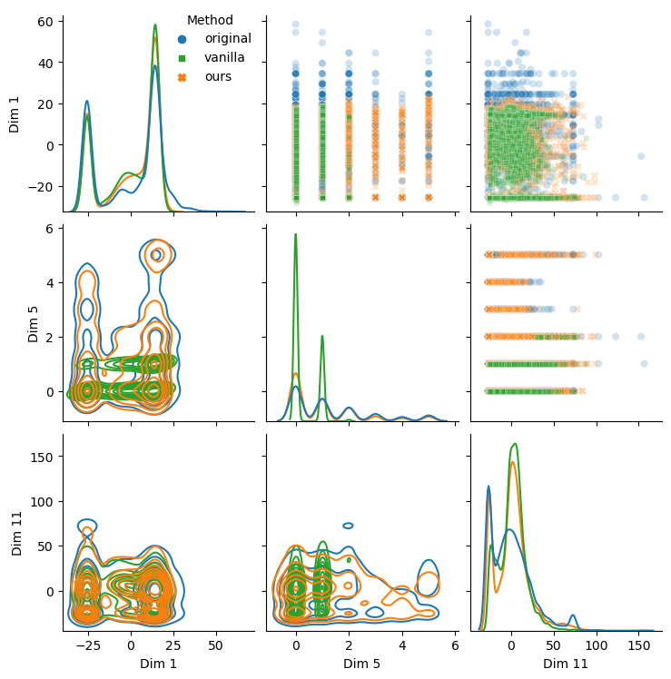
In addition to the results presented in the main paper, we present in Table 8 the same table as Table 1 but showing also the standard deviation of the results. Moreover, we show in Figs. 8 and 9 the full pair plot for the HI dataset, as well as another full pair plot of the labour dataset.

Table 8: Test reconstruction errors (mean and standard deviation) of different models and losses for the baseline and our framework.

Dataset	Method	VAE-ELBO	VAE-IWAE	VAE-DReG	HI-VAE
Adult	vanilla	0.21 $\pm$ 0.01	0.22 $\pm$ 0.02	0.24 $\pm$ 0.01	0.13 $\pm$ 0.00
Adult	ours	0.11 $\pm$ 0.02	0.12 $\pm$ 0.02	0.19 $\pm$ 0.08	0.09 $\pm$ 0.02
defaultCredit	vanilla	0.13 $\pm$ 0.00	0.14 $\pm$ 0.02	0.14 $\pm$ 0.01	0.15 $\pm$ 0.09
defaultCredit	ours	0.04 $\pm$ 0.00	0.05 $\pm$ 0.01	0.08 $\pm$ 0.01	0.06 $\pm$ 0.01
Wine	vanilla	0.09 $\pm$ 0.00	0.08 $\pm$ 0.00	0.08 $\pm$ 0.00	0.13 $\pm$ 0.01
Wine	ours	0.07 $\pm$ 0.01	0.07 $\pm$ 0.00	0.07 $\pm$ 0.00	0.11 $\pm$ 0.02
Diamonds	vanilla	0.19 $\pm$ 0.01	0.18 $\pm$ 0.01	0.18 $\pm$ 0.00	0.11 $\pm$ 0.02
Diamonds	ours	0.13 $\pm$ 0.02	0.12 $\pm$ 0.01	0.14 $\pm$ 0.01	0.01 $\pm$ 0.01
Bank	vanilla	0.20 $\pm$ 0.00	0.20 $\pm$ 0.00	0.19 $\pm$ 0.00	0.13 $\pm$ 0.02
Bank	ours	0.04 $\pm$ 0.00	0.10 $\pm$ 0.05	0.11 $\pm$ 0.04	0.10 $\pm$ 0.01
IMDB	vanilla	0.09 $\pm$ 0.02	0.10 $\pm$ 0.02	0.10 $\pm$ 0.02	0.08 $\pm$ 0.00
IMDB	ours	0.05 $\pm$ 0.04	0.05 $\pm$ 0.04	0.06 $\pm$ 0.04	0.10 $\pm$ 0.09
HI	vanilla	0.17 $\pm$ 0.01	0.16 $\pm$ 0.00	0.15 $\pm$ 0.00	0.11 $\pm$ 0.00
HI	ours	0.04 $\pm$ 0.00	0.04 $\pm$ 0.00	0.04 $\pm$ 0.00	0.11 $\pm$ 0.01
rwm5yr	vanilla	0.11 $\pm$ 0.01	0.09 $\pm$ 0.00	0.10 $\pm$ 0.00	0.04 $\pm$ 0.01
rwm5yr	ours	0.03 $\pm$ 0.00	0.03 $\pm$ 0.01	0.03 $\pm$ 0.00	0.02 $\pm$ 0.00
labour	vanilla	0.11 $\pm$ 0.00	0.10 $\pm$ 0.00	0.10 $\pm$ 0.00	0.10 $\pm$ 0.00
labour	ours	0.06 $\pm$ 0.00	0.07 $\pm$ 0.00	0.08 $\pm$ 0.01	0.07 $\pm$ 0.00
EL Nino	vanilla	0.10 $\pm$ 0.01	0.09 $\pm$ 0.00	0.08 $\pm$ 0.00	0.10 $\pm$ 0.01
EL Nino	ours	0.07 $\pm$ 0.01	0.06 $\pm$ 0.01	0.07 $\pm$ 0.00	0.02 $\pm$ 0.00
Magic	vanilla	0.06 $\pm$ 0.00	0.05 $\pm$ 0.00	0.05 $\pm$ 0.00	0.06 $\pm$ 0.00
Magic	ours	0.06 $\pm$ 0.00	0.05 $\pm$ 0.00	0.05 $\pm$ 0.00	0.03 $\pm$ 0.00
BooNE	vanilla	0.04 $\pm$ 0.00	0.04 $\pm$ 0.00	0.04 $\pm$ 0.00	0.04 $\pm$ 0.00
BooNE	ours	0.04 $\pm$ 0.00	0.04 $\pm$ 0.00	0.04 $\pm$ 0.00	0.04 $\pm$ 0.00

E.2 Multimodal experiments

E.2.1 Experiment details

For the multimodal experiments on MNIST-SVHN-Text, we have followed the same setup (including hyper-parameters) as Shi et al. 2019 and Sutter et al. 2021. We differ from their setups in that, in order to provide a fair comparison between losses, we always employ $K=30$ samples from ${\mathbf{Z}}$ , whether they are used as importance samples (IWAE, SIWAE) or used for the Monte-Carlo approximation of the expected value w.r.t. ${\mathbf{Z}}$ . Also, we do model selection using a validation dataset ( $10\%$ of the training data), and use a test set to obtain all the results presented in this work. Following Shi et al. 2019, we use the Sticking-The-Landing estimator (STL) (Roeder et al. 2017) for all losses. In short, this estimator simply omits the partial derivatives of the variational approximation w.r.t. the encoder parameters. Note that Shi et al. 2019 did not mention this estimator, but they rather talk about the DReG loss (Tucker et al. 2019). However, due to a bug in their code, they effectively compute the STL estimator in their experiments.

Selecting algorithm $f_{\psi}$ .

Since the number of impartiality blocks is large, and the training times are considerably longer than for the heterogeneous experiments, here we keep performing cross-validation, but this time we substitute grid-selection by hand-picked hyperparameters options that we observed to perform better than others (for example, we replaced IMTL-G (Liu et al. 2021b) by CAGrad (Liu et al. 2021a), as it was really clear by looking at the logs that IMTL-G was not working at all). Instead of looking for a specific algorithm for each of the impartiality blocks, we assume the same algorithm for all of them (same hyperparameters, but different parameters) and only cross-validate by using the modified backward pass on the blocks associated with the different goals in an incremental way (i.e., as presented in the inset table of Section 5 in the main paper).

Choosing the best algorithm in the multimodal setup is more complicated, as we care about different metrics (coherence and latent classification) at different levels (self and cross metrics), for each modality. We group all metrics in metric-type pairs (e.g., latent-classification-self), and within each group, we group them by the expert/modality they are testing (e.g., cross latent classification for the first expert tests all other latent samples in the classifier of the first expert). For each metric, we compute a value $I(x,y)$ , where $x$ is the value obtained by the algorithm, and $y$ the value obtained by the baseline, and take the average of each sequence recursively until obtaining a single number. We use the relative improvement $I(x,y)=\Delta(x,y)=\frac{x-y}{y}$ to compare the different metrics, choosing the method that obtains the best improvement, averaged across experts/modalities and metrics. For MVAE, we noticed that the metrics tend to oscillate and there are important trade-offs in performance. Therefore, for this model we adopt a more conservative approach and use $I(x,y)=\mathbf{1}_{x\geq y}$ , to choose the algorithm that, on average, improves the most number of metrics.

E.3 Additional experimental results

In this section, we have included the complete results for the MNIST-SVHN-Text experiments. Specifically, we present: the reconstruction coherence results for all the three losses (Table 9); the self and cross coherence results in tabular form for the three losses (Tables 10, 11 and 12), including extra information like the training times, the specific MTL algorithms used, and the goals for which we apply them; and the log-likelihoods conditioned on different modalities (Tables 13, 14 and 15), showing standard deviations as space permits, thus showing the high variance that the vanilla approach shows at times (for example, MoPoE in Table 15). Finally, we present the parallel coordinate plots for the three models (Fig. 10).

Table 9: Reconstruction coherence (

A=\{M,S,T\}

) for each modality, model, and dataset.

		ELBO			IWAE			SIWAE
	${\mathbf{x}}_{d}$	M	S	T	M	S	T	M	S	T
MVAE	vanilla	$97.528\,580\,427\,169\,8$	$88.261\,784\,315\,109\,25$	$99.303\,226\,470\,947\,27$	$97.269\,999\,980\,926\,51$	$87.194\,385\,528\,564\,46$	$98.755\,601\,644\,515\,99$	$97.373\,069\,524\,765\,01$	$87.474\,731\,206\,893\,92$	$98.829\,365\,968\,704\,22$
MVAE	ours	97.85028994083405	89.65040445327759	99.63676035404205	98.27756136655807	89.0097588300705	99.92557913064957	$97.416\,897\,118\,091\,58$	$87.627\,068\,161\,964\,42$	99.19884651899338
MMVAE	vanilla	$86.010\,034\,382\,343\,29$	$45.587\,326\,586\,246\,49$	$89.167\,807\,996\,273\,04$	$85.246\,920\,585\,632\,32$	$84.033\,243\,358\,135\,22$	$88.662\,599\,027\,156\,83$	$58.945\,936\,709\,642\,41$	$61.268\,170\,922\,994\,61$	$63.273\,503\,631\,353\,38$
MMVAE	ours	89.4158273935318	$45.831\,930\,637\,359\,62$	91.53931885957718	$87.552\,843\,491\,236\,36$	86.87140742937723	$90.932\,594\,736\,417\,14$	74.84600245952606	73.89406164487204	81.09348515669504
MoPoE	vanilla	$95.715\,466\,141\,700\,74$	$85.864\,113\,271\,236\,42$	$98.012\,429\,475\,784\,3$	$95.823\,138\,952\,255\,25$	$87.550\,030\,648\,708\,34$	$97.930\,523\,753\,166\,2$	$75.095\,855\,817\,198\,75$	$67.160\,804\,569\,721\,22$	$76.607\,539\,877\,295\,49$
MoPoE	ours	96.50165736675262	93.60147714614868	99.14027452468872	97.29161858558655	92.93432831764221	98.99884462356567	$96.913\,087\,368\,011\,47$	$89.013\,774\,693\,012\,24$	$99.284\,672\,737\,121\,58$

Table 10: Self and cross generation coherence (%) results for different models on MNIST-SVHN-Text, trained using ELBO and averaged over 5 different seeds. Models trained with our framework are able to sample more coherent modalities.

Self coherence

Cross coherence

{\bm{x}}_{d}

Time

A

S,T

M,T

M,S

MVAE

vanilla

∎

80.298\,466\,682\,434\,08

12.625\,821\,083\,784\,1

25.774\,458\,646\,774\,29

11.121\,198\,534\,965\,511

18.218\,290\,582\,299\,23

19.489\,357\,918\,500\,9

43.293\,524\,980\,545\,045

18.497\,849\,553\,823\,464

16.900\,739\,222\,764\,966

51.820\,915\,341\,377\,26

11.651\,328\,951\,120\,372

54.711\,379\,408\,836\,37

3.822\,388\,888\,888\,889\,3

CG (

\alpha=0.4

)

∎

\checkmark

∎

85.124\,324\,262\,142\,18

12.342\,862\,784\,862\,515

34.637\,197\,107\,076\,645

10.698\,623\,955\,249\,78

12.513\,992\,562\,890\,05

16.826\,085\,187\,494\,75

44.940\,358\,400\,344\,85

22.359\,844\,297\,170\,635

29.451550543308258

61.413\,592\,100\,143\,43

12.256\,772\,257\,387\,635

69.769\,041\,240\,215\,3

4.822\,986\,111\,111\,111\,4

MMVAE

vanilla

∎

95.2276736497879

68.253\,378\,570\,079\,8

99.988\,524\,615\,764\,62

62.927\,538\,156\,509\,4

99.922\,730\,028\,629\,3

81.426\,899\,135\,112\,76

31.055\,537\,611\,246\,11

37.424\,839\,287\,996\,29

34.235\,932\,677\,984\,24

96.272\,134\,780\,883\,79

71.286\,739\,408\,969\,88

83.788\,564\,801\,216\,13

10.069\,791\,666\,666\,667

CA (

\alpha=10.0

)

∎

\checkmark

∎

\checkmark

∎

\checkmark

92.622\,281\,610\,965\,73

73.83767068386078

99.985\,547\,363\,758\,09

76.00729763507843

99.592\,459\,201\,812\,74

87.79663294553757

29.111\,442\,714\,929\,58

34.457\,613\,527\,774\,81

31.780\,608\,743\,429\,184

95.268\,048\,346\,042\,63

79.34017926454544

87.30775266885757

13.057\,986\,111\,111\,11

MoPoE

vanilla

∎

94.523\,710\,012\,435\,91

71.207\,012\,236\,118\,32

99.989\,393\,522\,739\,41

66.803\,339\,123\,725\,89

99.979\,406\,595\,230\,1

98.120\,589\,554\,309\,84

19.697178527712822

33.247\,241\,377\,830\,505

31.550\,985\,574\,722\,29

96.79142832756042

77.040\,158\,212\,184\,91

97.15262800455093

23.244\,930\,555\,555\,555

CG (

\alpha=10

)

∎

\checkmark

∎

\checkmark

∎

\checkmark

94.644\,965\,231\,418\,61

73.35900366306305

100.0

74.75752681493759

99.978\,546\,798\,229\,22

98.423\,670\,232\,295\,99

15.842\,532\,366\,514\,2

32.836\,320\,251\,226\,425

31.034\,118\,682\,146\,07

96.033\,009\,886\,741\,64

78.60849350690842

96.666\,684\,746\,742\,25

29.412\,777\,777\,777\,777

Table 11: Self and cross generation coherence (%) results for different models on MNIST-SVHN-Text, trained using IWAE and averaged over 5 different seeds. Models trained with our framework are able to sample more coherent modalities.

Self coherence

Cross coherence

{\bm{x}}_{d}

Time

A

S,T

M,T

M,S

MVAE

vanilla

∎

87.326\,648\,235\,321\,05

11.699\,514\,538\,049\,693

37.492\,529\,153\,823\,85

10.758\,992\,880\,582\,804

26.63348317146301

29.478\,434\,324\,264\,524

54.097\,363\,352\,775\,57

25.163\,763\,910\,532

29.506\,842\,643\,022\,535

70.24494886398316

11.379\,081\,755\,876\,538

72.327\,798\,604\,965\,21

3.799\,555\,555\,555\,555\,6

GN (

\alpha=0.0

)

∎

\checkmark

∎

85.725\,106\,298\,923\,49

12.676\,706\,910\,133\,36

79.19154316186905

11.178\,777\,925\,670\,143

19.452\,513\,381\,838\,796

22.049\,068\,659\,543\,986

49.373\,075\,366\,020\,2

55.8295913040638

54.47539612650871

59.559\,909\,999\,370\,57

11.791\,023\,612\,022\,397

63.685\,056\,567\,192\,08

4.236\,666\,666\,666\,667

MMVAE

vanilla

∎

94.697\,476\,923\,465\,73

68.130\,804\,598\,331\,45

99.990\,360\,438\,823\,7

62.342\,401\,593\,923\,57

98.791\,582\,882\,404\,33

80.553\,266\,406\,059\,27

86.718\,530\,952\,930\,45

97.288\,332\,879\,543\,3

92.009\,593\,546\,390\,53

96.82694971561432

69.229\,179\,620\,742\,8

83.024\,583\,756\,923\,68

10.075\,486\,111\,111\,111

CG (

\alpha=0.4

)

∎

\checkmark

∎

94.961\,516\,062\,418\,61

73.661\,572\,734\,514\,86

99.991\,531\,173\,388\,15

68.489\,653\,865\,496\,31

99.24991031487784

83.849\,118\,153\,254\,18

88.98889621098837

97.97220627466837

93.48858892917633

96.269\,482\,374\,191\,28

76.549\,846\,927\,324\,92

86.400\,900\,284\,449\,25

11.958\,148\,148\,148\,15

MoPoE

vanilla

∎

94.444\,835\,186\,004\,64

63.162\,624\,835\,968\,02

99.974\,052\,608\,013\,16

58.200\,603\,723\,526

99.009\,869\,992\,733

99.242\,757\,260\,799\,41

80.754\,506\,587\,982\,18

94.764\,955\,341\,815\,95

88.623\,750\,209\,808\,35

96.514\,712\,274\,074\,55

66.131\,010\,651\,588\,44

96.034\,783\,124\,923\,71

23.2675

CG (

\alpha=10.0

)

∎

\checkmark

∎

\checkmark

∎

\checkmark

95.40619552135468

69.54438239336014

99.98906420707703

61.749\,838\,292\,598\,724

99.064\,502\,120\,018

99.065\,840\,244\,293\,21

81.226\,432\,323\,455\,81

96.4717224240303

92.98069477081299

96.635\,955\,572\,128\,3

73.32838028669357

96.161\,860\,227\,584\,84

29.347\,152\,777\,777\,774

Table 12: Self and cross generation coherence (%) results for different models on MNIST-SVHN-Text, trained using SIWAE and averaged over 5 different seeds. Models trained with our framework are able to sample more coherent modalities.

Self coherence

Cross coherence

{\bm{x}}_{d}

Time

A

S,T

M,T

M,S

MVAE

vanilla

∎

82.063\,213\,586\,807\,25

12.078\,495\,621\,681\,211

36.668\,736\,934\,661\,866

10.342\,429\,280\,281\,062

17.118\,748\,845\,532\,533

19.186\,700\,284\,481\,048

49.992\,209\,672\,927\,856

19.312\,240\,332\,365\,033

31.188\,021\,302\,223\,207

62.502\,512\,335\,777\,28

10.815\,181\,583\,166\,118

64.254\,502\,058\,029\,17

3.809\,166\,666\,666\,667

CG (

\alpha=0.4

)

∎

\checkmark

∎

86.888\,590\,455\,055\,24

12.894\,139\,252\,603\,05

59.14595350623131

10.990\,167\,409\,181\,59

20.918\,081\,700\,801\,85

30.335458368062973

54.827\,208\,817\,005\,16

31.816108897328377

24.968\,290\,328\,979\,492

71.867\,603\,063\,583\,37

11.104\,153\,469\,204\,898

72.741\,889\,953\,613\,28

4.770\,208\,333\,333\,334

MMVAE

vanilla

∎

95.89911252260208

48.302\,508\,518\,099\,785

53.021\,417\,930\,722\,24

28.433\,149\,680\,495\,26

52.515\,142\,038\,464\,55

40.454\,133\,972\,525\,59

84.443\,460\,404\,872\,89

51.076\,171\,174\,645\,41

67.768\,099\,904\,060\,36

96.80366516113281

39.960\,351\,958\,870\,89

68.380\,358\,815\,193\,18

10.067\,083\,333\,333\,333

CG (

\alpha=0.4

)

∎

\checkmark

∎

95.897\,186\,795\,870\,45

58.197\,258\,412\,837\,98

88.69847655296326

49.32506904006004

79.31589980920157

64.30353770653406

87.28511532147726

76.17471218109131

81.7105770111084

96.699\,014\,306\,068\,42

57.861\,342\,032\,750\,45

77.275\,938\,789\,049\,77

12.297\,916\,666\,666\,667

MoPoE

vanilla

∎

92.319\,706\,082\,344\,06

11.597\,061\,343\,491\,073

69.051\,729\,142\,665\,86

10.134\,417\,936\,205\,86

51.023\,241\,877\,555\,85

34.667\,880\,460\,619\,926

41.930\,220\,276\,117\,325

46.385\,733\,783\,245\,087

51.584\,096\,252\,918\,24

85.187\,664\,628\,028\,87

10.566\,544\,160\,246\,848

67.539\,525\,032\,043\,46

23.294\,722\,222\,222\,22

GN (

\alpha=0.5

)

∎

\checkmark

∎

90.991\,985\,797\,882\,08

11.996\,489\,390\,730\,854

83.81824642419815

10.6312271207571

62.753\,096\,967\,935\,56

52.083\,845\,436\,573\,03

28.190\,246\,224\,403\,376

46.905\,249\,357\,223\,51

43.344\,382\,941\,722\,87

79.640\,473\,425\,388\,34

10.814\,723\,558\,723\,92

90.325\,632\,691\,383\,36

24.575\,972\,222\,222\,22

Table 13: Log-likelihood of the joint generative model, conditioned on the variational posterior of subsets of the modalities. Results report on ELBO as loss function and are averaged over 5 different seeds. Each log-likelihood is divided by the dimensionality of its modality before adding them up, to better reflect improvement across modalities.

		$\mathbb{X}\|\text{M}$	$\mathbb{X}\|\text{S}$	$\mathbb{X}\|\text{T}$	$\mathbb{X}\|\text{MS}$	$\mathbb{X}\|\text{MT}$	$\mathbb{X}\|\text{ST}$	$\mathbb{X}\|\text{MST}$
MVAE	vanilla	$-8.61\pm 1.18$	$-10.26\pm 1.14$	$-8.17\pm 1.30$	$-8.18\pm 1.26$	$-1.51\pm 0.11$	$-7.41\pm 1.38$	$-1.02\pm 0.11$
MVAE	ours	$-8.07\pm 0.88$	$-9.89\pm 0.62$	$\mathbf{-6.94\pm 1.19}$	$-7.44\pm 0.64$	$-1.42\pm 0.05$	$-6.12\pm 1.69$	$-0.95\pm 0.00$
MMVAE	vanilla	$-2.30\pm 0.21$	$\mathbf{-2.18\pm 0.09}$	$-1.19\pm 0.00$	$\mathbf{-2.24\pm 0.11}$	$-1.75\pm 0.10$	$\mathbf{-1.68\pm 0.04}$	$\mathbf{-1.89\pm 0.07}$
MMVAE	ours	$-2.59\pm 0.40$	$-2.31\pm 0.13$	$\mathbf{-1.19\pm 0.00}$	$-2.45\pm 0.23$	$-1.89\pm 0.20$	$-1.75\pm 0.06$	$-2.03\pm 0.15$
MoPoE	vanilla	$-1.93\pm 0.01$	$-2.06\pm 0.04$	$-1.19\pm 0.00$	$-1.76\pm 0.00$	$-1.18\pm 0.00$	$-1.04\pm 0.00$	$-1.03\pm 0.05$
MoPoE	ours	$-1.92\pm 0.03$	$-2.09\pm 0.05$	$\mathbf{-1.19\pm 0.00}$	$-1.75\pm 0.02$	$-1.17\pm 0.01$	$\mathbf{-1.03\pm 0.00}$	$-1.00\pm 0.01$

Table 14: Log-likelihood of the joint generative model, conditioned on the variational posterior of subsets of the modalities. Results report on IWAE as loss function and are averaged over 5 different seeds. Each log-likelihood is divided by the dimensionality of its modality before adding them up, to better reflect improvement across modalities.

		$\mathbb{X}\|\text{M}$	$\mathbb{X}\|\text{S}$	$\mathbb{X}\|\text{T}$	$\mathbb{X}\|\text{MS}$	$\mathbb{X}\|\text{MT}$	$\mathbb{X}\|\text{ST}$	$\mathbb{X}\|\text{MST}$
MVAE	vanilla	$-8.62\pm 0.40$	$-10.68\pm 0.98$	$-6.78\pm 1.66$	$-8.28\pm 0.47$	$-1.83\pm 0.14$	$-6.08\pm 1.36$	$-1.15\pm 0.03$
MVAE	ours	$\mathbf{-8.26\pm 0.29}$	$\mathbf{-9.51\pm 0.25}$	$\mathbf{-2.83\pm 0.54}$	$\mathbf{-7.74\pm 0.15}$	$\mathbf{-1.35\pm 0.03}$	$\mathbf{-1.96\pm 0.33}$	$\mathbf{-0.94\pm 0.00}$
MMVAE	vanilla	$\mathbf{-1.98\pm 0.06}$	$-2.74\pm 0.32$	$-1.27\pm 0.00$	$-2.36\pm 0.15$	$\mathbf{-1.62\pm 0.03}$	$-2.00\pm 0.16$	$-1.99\pm 0.10$
MMVAE	ours	$-2.44\pm 0.03$	$\mathbf{-2.45\pm 0.12}$	$\mathbf{-1.26\pm 0.00}$	$-2.44\pm 0.06$	$-1.85\pm 0.01$	$\mathbf{-1.86\pm 0.06}$	$-2.05\pm 0.04$
MoPoE	vanilla	$\mathbf{-1.97\pm 0.00}$	$-2.55\pm 0.12$	$-1.27\pm 0.00$	$\mathbf{-5.85\pm 0.52}$	$-1.25\pm 0.00$	$-1.05\pm 0.00$	$-1.02\pm 0.00$
MoPoE	ours	$-2.01\pm 0.01$	$-2.61\pm 0.11$	$\mathbf{-1.27\pm 0.00}$	$-7.07\pm 0.06$	$\mathbf{-1.24\pm 0.01}$	$-1.05\pm 0.00$	$\mathbf{-1.01\pm 0.00}$

Table 15: Log-likelihood of the joint generative model, conditioned on the variational posterior of subsets of the modalities. Results report on SIWAE as loss function and are averaged over 5 different seeds. Each log-likelihood is divided by the dimensionality of its modality before adding them up, to better reflect improvement across modalities.

		$\mathbb{X}\|\text{M}$	$\mathbb{X}\|\text{S}$	$\mathbb{X}\|\text{T}$	$\mathbb{X}\|\text{MS}$	$\mathbb{X}\|\text{MT}$	$\mathbb{X}\|\text{ST}$	$\mathbb{X}\|\text{MST}$
MVAE	vanilla	$-8.82\pm 0.63$	$-10.13\pm 0.29$	$-7.17\pm 1.73$	$-8.52\pm 0.74$	$-2.23\pm 1.31$	$-5.94\pm 1.35$	$-1.15\pm 0.02$
MVAE	ours	$-8.41\pm 0.14$	$-10.52\pm 0.53$	$-5.65\pm 1.76$	$-8.13\pm 0.17$	$-1.46\pm 0.07$	$-5.49\pm 1.87$	$\mathbf{-1.01\pm 0.01}$
MMVAE	vanilla	$\mathbf{-2.01\pm 0.08}$	$-4.04\pm 0.43$	$-3.25\pm 0.94$	$-3.02\pm 0.20$	$-2.63\pm 0.49$	$-3.64\pm 0.25$	$-3.10\pm 0.18$
MMVAE	ours	$-2.34\pm 0.36$	$-3.22\pm 1.28$	$-3.03\pm 1.07$	$-2.78\pm 0.59$	$-2.69\pm 0.54$	$\mathbf{-3.12\pm 0.43}$	$\mathbf{-2.86\pm 0.22}$
MoPoE	vanilla	$-6.29\pm 2.75$	$-10.02\pm 0.43$	$-3.80\pm 1.48$	$-7.51\pm 0.93$	$-1.59\pm 0.35$	$-4.97\pm 2.68$	$-3.15\pm 3.78$
MoPoE	ours	$-8.01\pm 0.42$	$-10.16\pm 0.55$	$-2.96\pm 1.11$	$-7.26\pm 0.28$	$-1.34\pm 0.01$	$\mathbf{-2.30\pm 0.91}$	$-0.99\pm 0.02$

Mitigating Modality Collapse in Multimodal VAEs via Impartial Optimization

Abstract

Keywords:

1 Introduction

2 Preliminaries

2.1 State-of-the-art

3 Impartial Optimization in Multimodal VAEs

3.1 Our Approach

3.2 Conflicting Gradients Solutions

4 Extending Our Framework

4.1 Heterogeneous VAE Models

4.2 Multimodal VAE Models

4.2.1 Mixture-based VAEs for Multimodal Data

4.2.2 Impartial Optimization

5 Experiments

5.1 Heterogeneous Data

5.2 Multimodal Data

6 Conclusions

7 Acknowledgements

References

Appendix A Multitask learning and conflicting gradients

A.1 Conflicting-gradient solutions

Appendix B Alleviating modality collapse

Appendix C Dominance of Poisson likelihoods

Computing the expected squared norms.

Bounding the norms under our working pipeline.

Appendix D Model descriptions

D.1 Variational autoencoder (VAE)

Loss.

Imputation.

D.2 Importance weighted autoencoder (IWAE)

Loss.

D.3 Doubly reparametrized gradient estimator (DReG)

Encoder loss.

D.4 HI-VAE

Loss.

D.5 Mixture-based VAEs

Appendix E Experimental details

E.1 Heterogeneous experiments

E.1.1 Dataset descriptions

Datasets.

Preprocessing.

E.1.2 Experimental settings

Model selection.

Selecting the algorithm fψf_{\psi}.

Statistical test.

Data Generation.

E.1.3 Additional experimental results

E.2 Multimodal experiments

E.2.1 Experiment details

Selecting algorithm fψf_{\psi}.

E.3 Additional experimental results

Mitigating Modality Collapse in Multimodal VAEs
via Impartial Optimization

Selecting the algorithm $f_{\psi}$ .

Selecting algorithm $f_{\psi}$ .