Causality, unitarity and stability in quantum gravity:
a non-perturbative perspective
Abstract
Resumming quantum fluctuations at the level of the gravitational path integral is expected to result in non-local effective actions and thus in a non-trivial momentum dependence of the propagator. Which properties the (dressed) graviton propagator has to satisfy and whether they can all be met are key open questions. In this work we present criteria and conditions for the momentum dependence of a graviton propagator which is consistent with unitarity, causality, and stability in a non-perturbative setting. To this end, we revisit several aspects of these conditions, highlighting some caveats and subtleties that got lost in recent discussions, and spelling out others that to our best knowledge have not been studied in detail. We discuss the consequences of these concepts for the properties of the graviton propagator. Finally, we provide examples of propagators satisfying unitarity and causality, while avoiding tachyonic and vacuum instabilities, and allowing for an analytic Wick rotation.
1 Introduction
The conundrum of quantum gravity (QG) originally arose as a fundamental incompatibility between renormalizability and unitarity in the perturbative quantization of Einstein-Hilbert tHooft:1974toh; Goroff:1985sz; Goroff:1985th; vandeVen:1991gw and quadratic gravity Stelle:1977ry. Subsequent attempts to reconcile unitarity and renormalizability resulted in a proliferation of different approaches to the problem of QG.
The formulation of the Standard Model of particle physics was crucially driven by the interplay between theoretical ideas and experimental tests: inputs from the theory drove the experiments, and the experiments constrained the models and tested their assumptions. QG lives in a different universe: quantum gravitational effects may be too tiny to be directly detected in experiments. Discriminating between different proposals based on observations appears currently out of reach. Lacking experiments, theoretical investigations of the quantum aspects of gravity grope in the dark. Consistency, which is far from being trivial in the realm of QG, becomes a key requirement to guide theoretical studies.
First of all, a fundamental quantum theory of gravity ought to be renormalizable: it must be predictive, delivering (finite) observables parametrized by a few free parameters only. In the modern, Wilsonian understanding of renormalization Wilson:1973jj, the renormalization group (RG) trajectory of a renormalizable quantum field theory (QFT) ends up in a (free or interacting) fixed point in the ultraviolet (UV), and the number of free parameters of the theory is dictated by the codimension of its critical hypersurface. Power counting suggests that Einstein gravity cannot be asymptotically free, due to the negative mass dimension of the Newton coupling. Nonetheless, the existence of an “asymptotically safe” (i.e., interacting) fixed point for gravity 1976W—whether fundamental or stemming from string theory deAlwis:2019aud; Basile:2021euh—remains a compelling possibility Eichhorn:2017egq; Donoghue:2019clr; Pawlowski:2020qer; Bonanno:2020bil, which can be investigated using, e.g., lattice techniques Laiho:2016nlp; Loll:2019rdj or the Functional Renormalization Group (FRG) Dupuis:2020fhh11 1 In an RG setup, the bare action is not guessed, rather, it is derived as an UV fixed point of the RG flow (modulo reconstruction problem Manrique:2008zw; Morris:2015oca; Fraaije:2022uhg). The FRG has proven useful in several approaches to QG, including asymptotically safe gravity Souma:1999at; Lauscher:2002sq; Litim:2003vp; Codello:2006in; Machado:2007ea; Benedetti:2009rx; Manrique:2011jc; Dietz:2012ic; Ohta:2013uca; Dona:2013qba; Codello:2013fpa; Christiansen:2014raa; Falls:2014tra; Becker:2014qya; Christiansen:2015rva; Meibohm:2015twa; Oda:2015sma; Biemans:2016rvp; Eichhorn:2016esv; Falls:2016msz; Gies:2016con; Biemans:2017zca; Christiansen:2017cxa; Hamada:2017rvn; Platania:2017djo; Falls:2017lst; Eichhorn:2018nda; Eichhorn:2019yzm; Knorr:2021slg; Baldazzi:2021orb; Bonanno:2021squ; Fehre:2021eob; Knorr:2022ilz, unimodular quantum gravity Eichhorn:2013xr; deBrito:2019umw; deBrito:2020rwu; deBrito:2020xhy, Hořava–Lifshitz gravity Contillo:2013fua; DOdorico:2015pil, Lorentz-symmetry-violating models Knorr:2018fdu; Eichhorn:2019ybe, matrix and tensor models Eichhorn:2013isa; Eichhorn:2017xhy; Eichhorn:2018phj; Eichhorn:2019hsa, group field theory Benedetti:2015yaa; Geloun:2016qyb; BenGeloun:2018ekd; Lahoche:2018hou; Pithis:2020kio and string theory deAlwis:2019aud; Basile:2021euh; Basile:2021krk; Basile:2021krr; Gao:2022ojh; Ferrero:2022dpk. Crucially, the FRG can be used as an alternative to the path integral to compute the quantum effective action Codello:2015oqa; Knorr:2018kog; Knorr:2019atm; Ohta:2020bsc; Bonanno:2021squ; Knorr:2021niv. In turn, the quantum effective action can be exploited to connect first-principle computations in QG with experiments and observations, e.g., to explore quantum corrections to cosmological and black-hole spacetimes (see Bonanno:2006eu; Falls:2012nd; torres15; Koch:2015nva; Bonanno:2015fga; Bonanno:2016rpx; Kofinas:2016lcz; Falls:2016wsa; Bonanno:2016dyv; Bonanno:2017gji; Bonanno:2017kta; Bonanno:2017zen; Bonanno:2018gck; Liu:2018hno; Majhi:2018uao; Anagnostopoulos:2018jdq; Adeifeoba:2018ydh; Pawlowski:2018swz; Gubitosi:2018gsl; Platania:2019qvo; Platania:2019kyx; Bonanno:2019ilz; Held:2019xde; Bosma:2019aiu; Knorr:2022kqp for some simple models and Bonanno:2017pkg; Platania:2020lqb for reviews), and to compute scattering amplitudes Draper:2020bop; Draper:2020knh; Knorr:2020bjm; Ferrero:2021lhd; Knorr:2022lzn. Finally, the knowledge quantum effective action is paramount to establish whether the theory satisfies all known consistency criteria.
Indeed, beyond renormalizability, a consistent theory of QG ought to preserve at least some of the properties of (local) QFTs, such as causality, unitarity and stability. In the context of effective field theories (EFT), these conditions have been translated in strong and very precise bounds on the Wilson coefficients Adams:2006sv; Cheung:2016yqr; Bellazzini:2016xrt; deRham:2017zjm; deRham:2017xox; deRham:2018qqo; DeRham:2018bgz; Alberte:2019lnd; Alberte:2019xfh; Alberte:2019zhd; Alberte:2020bdz; Alberte:2020jsk; deRham:2021fpu; Herrero-Valea:2022lfd; deRham:2022hpx. Yet, their non-perturbative realization beyond an EFT setup requires accounting for the momentum dependence of couplings (aka, the form factors Knorr:2019atm) in the quantum effective action. Logarithmic form factors stemming from perturbative computations at one-loop order are the simplest realization of this momentum dependence, and their presence already brings important consequences for unitarity, causality and stability Donoghue:2018lmc; Donoghue:2019ecz; Donoghue:2019fcb; Donoghue:2021meq. Going beyond one-loop order, the form factors can be much more complicated and ultimately ought to be derived by integrating out all quantum gravitational fluctuations, e.g., at the level of the path integral or using the FRG. In particular assessing unitarity, as well as causality and stability, requires investigating the effective action beyond a polynomial expansion in momenta Wetterich:2019qzx; Draper:2020bop; Platania:2020knd; Knorr:2021niv; Bonanno:2021squ; Fehre:2021eob, since such truncations can potentially generate fictitious poles Kuntz:2019qcf; Platania:2020knd.
The goal of the present work is to determine conditions for the non-perturbative realization of causality, unitarity and stability, in particular at the level of the dressed graviton propagator, and to introduce models satisfying all of them while allowing for an analytic Wick rotation. To this end, we first revisit various aspects of (non-perturbative) unitarity, causality and stability, we examine some of their caveats and subtle details, and discuss their applicability to QG. Specifically, in Sect. 2 we argue why (non-perturbative) unitarity is generally best studied at the level of the effective action. Approximations to the effective action based on truncated derivative expansions naturally lead to the appearance of fictitious poles in the dressed propagator. The resulting fake ghosts decouple dynamically when a sufficiently high number of operators is considered, in that the modulus of their initially-negative residue decreases and vanishes in the limit where no approximation is employed Platania:2020knd. We discuss this residue decoupling mechanism in Sect. 3, and we provide further numerical evidence of its validity in the case of effective actions constructed with various entire and non-entire form factors. Next, in Sect. 4 we collect and analyze various notions and definitions of causality that have appeared in the literature, and attempt to clarify their relation. We also discuss tachyonic and vacuum (in)stabilities, differentiating between the way they arise classically and at the quantum level. In this course, we also highlight that the tachyonic case comes with several ambiguities, and that tachyonic instabilities are not necessarily problematic, since in some cases they can be cured by the interaction terms in the quantum effective action. We show this by providing some arguments and also by constructing an explicit example for a scalar model. In the context of causality, we pick the definition of microscopic causality discussed in Donoghue:2019fcb, which is based on the structure of the Fourier modes of the propagator, and we generalize the analysis from the case of unstable ghosts studied in Donoghue:2019fcb to the case of a general propagator. The types of poles and their implications for unitarity, causality and stability are summarized in Tab. 2. Our analysis indicates that to avoid acausalities and (tachyonic and vacuum) instabilities, the dressed propagator should be free from complex-conjugate poles and poles with negative width. In addition, to allow for an analytic Wick rotation no essential singularities should occur. In Sect. 5, we highlight that logarithmic quantum corrections that naturally arise at the level of the gravitational effective action can only alleviate some problems, but are not enough to retain unitarity, causality and stability. This motivates our study in Sect. 6, where we construct models where causality, unitarity, stability and analytic continuation can all be preserved. Interestingly, the common feature of these models is the presence of branch cuts. We summarize our findings in Sect. 7.
2 Non-perturbative unitarity, effective actions, and the RG
In this section we review some basic concepts intertwined with unitarity, that will be useful throughout the manuscript, including the notion of unstable particle and how it is related to quantum effects, the optical theorem and its non-perturbative character, and the role of quantum effective actions.
2.1 Non-perturbative character of the optical theorem and spectral density
In the context of QFT the condition that the S-matrix is unitary, , implies the optical theorem: for any initial state and final state , the transfer matrix – defined by – satisfies the relation
| (1) |
For a unitary theory the right-hand side of this equation has to be positive for any initial and final state.
While one could use perturbation theory to expand the left- and right-hand sides of the optical theorem (provided that this perturbative expansion does not break down at any scale) and verify unitarity order by order, this is not necessary if the quantum effective action is known. In fact, any scattering amplitude can be computed from the functional derivatives of the effective action according to
| (2) |
where are interacting quantum fields and is the vacuum of the fully-interacting theory. Therefore, the optical theorem does not need perturbation theory, rather it can be seen as a set of non-perturbative relations between scattering amplitudes and cross sections. In particular, if the effective action is known, one could in principle use it to evaluate and verify that it is positive for any initial and final states.
On the right-hand side of Eq. (1), one can insert an identity operator to express as a sum over all possible intermediate states
| (3) |
The unitarity condition thus holds if there are no negative-norm states (ghosts) in the set of all possible asymptotic states. Indeed, if ghosts exist in the spectrum of the theory, the space of asymptotic states is no longer complete, i.e., it is no longer a Fock space. In this case the “identity” would carry some minus signs that would also enter the sum in Eq. (3). Unitarity thus has to do with the field content of the theory. In the context of QFT, this information is encoded in (the pole structure of) the dressed propagator , where denotes a tensorial structure and is the correspondent scalar part. For a unitary theory the corresponding spectral density,
| (4) |
has to be real and positive definite (at least for asymptotic states, see the discussion in Sect. 2.4). Indeed, for the optical theorem yields relations of the form , where is the transition amplitude . Specializing to the case where is a one-particle state, one finds that (i) the optical theorem entails a non-trivial relation between the spectral density and the vertices of the theory, and that (ii) the unitarity condition implies the positivity of .
A dressed propagator can in principle feature multiple poles, each one corresponding to a degree of freedom of the theory. Assuming that each of these poles has multiplicity one, the contribution of each pole and/or branch singularity to the propagator can be isolated with the aid of the Cauchy integral formula. The propagator can thus be written as a sum of single-pole propagators and, possibly, a continuum part. In what follows we will work in Lorentzian signature, using the mostly negative convention (+ - - -), and we will assume that has no essential singularities invalidating the use of the Cauchy formula. For a scalar propagator with a single branch cut on the real axis22 2 Let us remark that, in principle, there could be multiple branch cuts, and they do not generally lie on the real axis. An example of this situation will be presented in Sect. 6.
| (5) |
where are renormalized masses, and for , with being a threshold mass for the production of a resonance or a multi-particle state. The integration contour is shown in Fig. 1.
Eq. (2.1) is the most general form of a dressed propagator. There can be contributions from stable particles (ghosts) and possibly bound states, characterized by isolated poles with positive (negative) residues. Pairs of complex-conjugate poles would appear in the form of isolated pairs of poles coming with complex-conjugate masses and residues. The residues of the complex-conjugate poles must be complex conjugates themselves to preserve the reflection-positivity condition of the propagator, . Finally, unstable particles or multi-particle states correspond to branch cut singularities above or below a threshold mass .
The total spectral density reads
| (6) |
The contribution of complex-conjugate poles to the spectral density cancels out, implying that they do not affect unitarity. Stable particles/ghosts contribute with Dirac deltas in the expression of the spectral density. Unstable particles/ghosts contribute instead with a continuum part . Unitarity thus holds if
| (7) |
namely, if there are no stable ghosts, and if unstable ghosts come in the form of Merlin modes Donoghue:2019ecz; Donoghue:2019fcb. These conditions guarantee that the spectral density is positive. Moreover, the spectral density must be real and the normalization condition
| (8) |
is to be imposed.
The Källen-Lehmann spectral representation of the (dressed) propagator Kallen:1952zz; Lehmann:1954xi, from which Eq. (4) follows, is very general and does not rely on any perturbative expansion. It encodes all-order, non-perturbative information on the dressed propagator, and thereby on the degrees of freedom of the full theory. The spectral density can be derived from the dressed propagator, which in turn can be computed from the effective action . This makes the quantum effective action crucial to establish unitarity in non-perturbative QFTs, and a useful tool in the case of QFTs which are perturbative at all scales.
2.2 Effective actions and the renormalization group
The effective action is obtained by integrating out all quantum fluctuations at the level of the functional integral. One possible way to obtain is via the FRG equation Wetterich:1992yh; Morris:1993qb; Reuter:1993kw; Reuter:1996cp
| (9) |
Here is the so-called effective average action. At the level of the path integral, it can be thought of as the effective action obtained by the integration of fluctuations with momenta . Its variation with respect to the RG scale is induced by the variation of the infrared regulator and by the corresponding RG-scale dependent inverse propagator. The supertrace Str stands for both a sum over discrete indices and an integral over continuum variables, i.e., either momenta or spacetime coordinates. The RG flow of connects smoothly the UV regime, where approaches a bare (fixed point) action , and the infrared limit , where all fluctuations are integrated out. In the latter limit, reduces to the quantum effective action .
The effective average action contains all invariants according to the underlying symmetries. In the infrared limit , as a result of the integration of fluctuations along all momentum scales, the quantum effective action is expected to be non-local. This is the case even at the one-loop level, where the integration of fluctuating modes give rise to logarithmic corrections to the classical action.
One of the challenges of the FRG approach to QG is the impossibility to solve Eq. (9) exactly. In order to obtain an approximate solution to this equation and investigate the UV completion of the theory, one has to resort to “truncations” of the theory space: an ansatz for is chosen, that includes a manageable number of operators. The effective average action is expanded using, e.g., a derivative expansion, and then this expansion is truncated to a finite truncation order to make the computation of the beta functions feasible. On the one hand, this method is useful to determine some key features of the RG flow of , such as its fixed points and universality properties. On the other hand, this method does not allow to infer the unitarity of the theory. In fact, if a derivative expansion of is truncated at a finite order, the corresponding propagator derived in the limit displays a finite number of unphysical poles Platania:2020knd. As we will explain in detail in the next section, reinforcing the arguments in Platania:2020knd, establishing unitarity in QFT requires the knowledge of the full effective action, as truncations of its derivative expansion would lead to the appearance of unphysical poles.
2.3 Absorptive part of the dressed propagator and unstable particles
We have argued that the full spectral density is to be computed using the dressed propagator, which in turn can be derived from the effective action .
Beyond being convenient, in some cases using fully-dressed quantities (aka, resumming all quantum effects) is crucial to count the degrees of freedom of a theory correctly Fradkin:1981vx. Quantum effects can for instance make a particle appearing in the bare theory unstable Fradkin:1981vx; Donoghue:2019fcb, thus removing it from the spectrum of asymptotic states Veltman:1963th. In what follows we review this mechanism using a simple example.
Starting from the bare theory of a single scalar particle with bare mass , resumming quantum effects would generally lead to a dressed propagator of the form
| (10) |
Here is the self-energy generated by vacuum polarization. The (bare) Feynman propagator has a pole at . Turning interactions on, if does not lead to extra poles other than the one present in the bare theory, quantum effects can renormalize the mass and can also make the particle unstable. This happens when the self-energy has an imaginary part, as it gives the particle a non-zero decay width. The renormalized mass is defined by the condition , while the imaginary part of is related to the total decay rate of the particle. Let us assume that does not add extra poles. In this case, the sum over all cuts on the right-hand side of the optical theorem reads
| (11) | ||||
where we have omitted the dependence of on for shortness. The sum above defines the absorptive part of the propagator and, for a theory with one single pole, the result depends on whether vanishes or not. In particular
| (12) |
being the residue at the corresponding pole. In the case , provided that , the absorptive part of the propagator corresponds to an intermediate (stable) one-particle state with mass . In the case , quantum effects have made the particle of mass unstable, so that the first term in the absorptive part of the propagator vanishes. The spectral density, which is proportional to the absorptive part of the propagator, thus depends crucially on the form of the self-energy .
Since unstable particles are not part of the space of asymptotic states Veltman:1963th, they do not contribute to the sum in Eq. (3). Consequently, determining which degrees of freedom enter the sum over intermediate states in the optical theorem requires resumming quantum fluctuations first. Note that perturbative expansions break down in the branch cut regions, so that describing unstable particles requires all-order, non-perturbative effects. This motivates further the use of dressed quantities to assess the unitarity of QFTs.
2.4 Discussion and assumptions
Let us end this section with some words of caution.
The arguments reviewed in this section are well understood in the context of QFTs of matter, but generally get more involved in the context of gauge theories. In particular, it is not yet clear whether and under which conditions the spectral density of a gauge field has to be positive. For instance, QCD is expected to be unitary, but the spectral density arising from the gluon propagator is not positive definite Hayashi:2018giz; Kondo:2019ywt. Similarly, in gravity the conformal mode is a ghost, at least classically. These examples highlight that the question of unitarity and its relation with the positivity of the spectral density are crucially intertwined with the spectrum of asymptotic states: the only dangerous “minus signs” that can enter the optical theorem are those associated with negative-norm asymptotic states—those contributing to the sum in Eq. (3). Going back to the question of QCD, due to confinement the gluon ought not to be part of the Fock space, and this could make the negativity of the gluon spectral density irrelevant for unitarity in QCD. Likewise, for QG the conformal mode is not an on-shell mode.
On top of this, in the context of QG one might even fail to find a suitable definition of unitarity Platania:2020knd. For instance, if gravity is interacting in the UV, the standard concept of an asymptotic state would cease to make sense. In addition, the definition of asymptotic states requires the knowledge of the (true) vacuum of the theory and determining it is expected to be highly non-trivial Bonanno:2013dja. Finally, if fluctuations of the spacetime signature can take place, unitarity itself would become meaningless.
Addressing these issues goes well beyond the scope of this work, and we will refrain from discussing them again in the remainder of this paper.
In the following we will limit ourselves to a discussion of the constraints on the transverse-traceless (TT) part of the graviton propagator, assuming that its poles define the asymptotic states of the theory.
Based on the considerations of this section, (non-perturbative) unitarity is better studied at the level of the effective action. To preserve unitarity the dressed (graviton) propagator should not have real poles with negative residue.
3 Fictitious ghosts in “truncated” field theories and the residue conjecture
In this section we show that truncating the derivative expansion of an effective action to a finite order generally produces fake ghosts, i.e., ghosts that are artifacts of the approximations and that do not appear in the full theory. The fake ghosts decouple dynamically for sufficiently large truncations, as their residues vanish.
As a toy model for the effective action, we shall consider a non-local effective action interpolating between QED and Lee-Wick QED. The reason is twofold: first, unitarity in QED is better under control than in QG, where even the precise definition of unitarity is unclear. Second, as we shall see explicitly in Sect. 5, the propagators of Lee-Wick QED and one-loop QG share very similar properties (cf. Fig. 15).
3.1 A toy model for QED and Lee-Wick QED
Starting from the classical QED action
| (13) |
and integrating out one or more massive degrees of freedom, one typically obtains a non-local effective action whose quadratic part reads
| (14) |
with . The latter has to be complemented with a gauge fixing term,
| (15) |
and the resulting propagator on Minkowski spacetime reads
| (16) |
In what follows we shall fix . Following LandauD; Donoghue:2015nba; Donoghue:2015xla, in the one-loop approximation, the function for QED can be obtained by integrating out a scalar or fermionic degree of freedom, and it reads LandauD
| (17) |
where is the fine structure constant and is the mass of the degree of freedom which has been integrated out. In the case of Lee-Wick QED, the form of the function is instead Boulware:1983vw; Donoghue:2018lmc
| (18) |
where corresponds to the threshold of production of a fermion-antifermion pair (or a pair of scalars) and is a cutoff scale. The momentum-space propagator can be written as33 3 A detailed explanation of the origin of this equation and its regime of validity are reported in Sect. 5, where we study logarithmic interactions of the Lee-Wick and one-loop quantum-gravity type, cf. Eq. (73).
| (19) |
The absorptive part of the scalar part of the propagator thus reads
| (20) |
with
| (21) |
Its structure is similar to that in Eqs. (11)-(12). The first term corresponds to the standard photon propagator, the second describes the propagation of an unstable ghost, includes fermionic/scalar loops, and contributes when . Diagrammatically
![[Uncaptioned image]](2206.04072v2/Images/diagram4.png)
For a dressed propagator with one single pole, only one of the two terms on the right-hand side is realized. The first term arises in the case of a theory with one single, stable degree of freedom, the second one describes an unstable degree of freedom. We note here that if the dressed propagator is computed from a one-loop effective action, the gray bubble in the right-hand-side is the sum of all possible processes involving one loop of the integrated-out degrees of freedom. For theories with multiple poles both types of terms on the right-hand side could arise.
In the following we shall employ the generalized propagator
| (22) |
which reproduces the propagator of one-loop QED for and the case of Lee-Wick QED for (cf. Tab. 1). The one-loop QED propagator has no poles beyond the massless one for small . The branch cut along is related to the threshold of production of lighter particles. However, there is also a tachyonic ghost pole at (the Landau pole), beyond which the theory breaks down. In the case of Lee-Wick QED, as explained in Sect. 5, there is an unstable ghost pole, whose real part lies in the branch cut region, and a pair of complex-conjugate poles. The pole structure is thus very similar to that of one-loop QG, cf. Sect. 5. Finally, if is taken to be negative, the ghost pole is shifted out of the branch cut region, where the logarithmic propagator is real. This makes the ghost stable, and entails a violation of unitarity. The spectral densities corresponding to these three cases are depicted in Fig. 2.
| Theory | Couplings | Real poles |
|---|---|---|
| One-loop QED | , | Landau pole LandauD |
| Standard Lee-Wick QED | , | Unstable ghost Boulware:1983vw; Donoghue:2018lmc |
| Lee-Wick QED, non-standard sign | , | Stable ghost |


Taking (14) as a toy model for the effective action, with
| (23) |
the propagator in Eq. (22) provides us with a toy model for the fully dressed photon propagator. Along the lines of Platania:2020knd, in the next subsection we will study the pole structure of this propagator varying the truncation order of the effective action in a derivative expansion.
3.2 Polology of the expanded one-loop effective action
Truncating the derivative expansion of the effective action (14), one obtains a “truncated” inverse propagator of the form (16), with
| (24) |
being defined as . Such an expansion of the effective action cannot reproduce all features of the “full theory” (14) since some physical effects, including the possibility of making a particle unstable, rely on non-perturbative features of the theory. In particular, although the function in Eq. (23) has at most one real massive zero (cf. Tab. 1), its truncated version can have several. The scalar part of the truncated propagator,
| (25) |
thus generally has a number of real and complex-conjugate poles (plots in the left column of Fig. 3). These poles are generated by the convergence properties of the derivative expansion of (plots in the right column of Fig. 3). This can be seen by studying the sequence of approximated functions for increasing values of . For large and negative , the behavior of is dominated by the term . Depending on the sign of the coefficient and on whether is even or odd, can either diverge negatively or positively as . Specifically, due to the structure of the function , in the region the function alternates between positive and negative signature divergences, with a certain periodicity in (see plots in the right column of Fig. 3). The convergence properties of can thus lead to accidental zeros for , and the corresponding truncated propagator develops a number of fictitious complex-conjugate and real poles. The disappearance of these fictitious zeros of can only be achieved in the limit .


Since the function truncated to order is polynomial, and
| (26) |
some of the aforementioned fictitious degrees of freedom must be ghosts. Specifically, in the cases at hand, the truncated derivative expansion generates several complex-conjugate poles and one single fake (tachyonic) ghost. As is apparent from Fig. 3 (left column), the corresponding zero is generated at large negative for low-order truncations, but moves towards for increasing values of . In other words, it seems that fictitious zeros move towards and accumulate on the boundary of the domain of convergence of . It is worth noticing that if the resummation of quantum fluctuations yields a non-local effective action with given by an entire function, the radius of convergence is infinity and fictitious ghost poles are expected to approach infinity for increasing values of . We will come back to this point in the next subsection.
The domain of convergence and branch cut region of are shown in Fig. 4.
Fake degrees of freedom live outside the domain of convergence of the -function, but appear in the principal branch of the logarithmic interaction, and approach its boundary for increasing values of . Possible unstable ghosts in the full theory can only live in the branch cut region. The latter region cannot overlap with the domain of converge of the full -function by construction. Thus, unstable ghosts (or particles) cannot be captured using the truncated expansion (24) of the inverse propagator (see Fig. 5).


More precisely, the radius of convergence is finite due to the breakdown of perturbation theory near the mass of an unstable particle Veltman:1963th. Indeed, this is because the truncated propagator is a finite sum of single-pole propagators, and the corresponding spectral density is thereby a sum of Dirac deltas only. Consequently, the spectral function computed from a truncated version of the theory (cf. Fig. 5), beyond not being positive due to the presence of fake ghosts, does not have the continuum part associated with the resonance.
Due to their negative residues, the fake degrees of freedom contribute to the truncated spectral function with negative-diverging Dirac deltas. However, since the fake ghosts are not part of the set of asymptotic states of the full theory, they must dynamically decouple by increasing the truncation order . As argued in Platania:2020knd, it might be possible to determine the nature of a ghost in a truncated theory by studying the behavior of the corresponding residue with . In fact, the residue associated with fake ghosts seems to vanish for sufficiently large , at least in the case of QED and Lee-Wick QED with non-standard sign Platania:2020knd, while the residue of a ghost appearing in the full theory is negative and remains negative for any (cf. Fig. 6).


In the cases at hand, the contribution of fictitious ghost poles to the propagator (and thus to the optical theorem) becomes small for sufficiently large and vanishes for , so that fake ghosts decouple in the limit where no approximation is employed. In what follows we will refer to this as the residue decoupling mechanism of fake ghosts.
Since quadratic gravity Stelle:1977ry can be viewed as a truncation of a full diffeomorphism-invariant theory of QG, e.g., within the framework of asymptotically safe gravity, the massive ghost of quadratic gravity could be a fake degree of freedom, rather than a problem of the theory. In particular, if the residue decoupling mechanism holds, it can be used to investigate this hypothesis. This provides an important motivation to further explore the validity of the residue decoupling mechanism.
3.3 Residue decoupling mechanism of fake poles: further numerical evidence
In the case of logarithmic effective actions, the (absolute value of the) residue of fictitious ghosts decreases as the truncation order is increased, while for genuine ghosts the residue is negative and quickly converges to a finite (negative) value. It is both instructive and useful to investigate the validity of this statement in the case of other form factors .
Our numerical results are summarized in Fig. 7 for a sample of -functions. The residue mechanism holds in all these examples, which include both entire and non-entire functions. In the case of entire functions, however, the convergence of the sequence of residues is slower than in the case of non-entire functions.


It is straightforward to apply the same analysis to other -functions, such as trigonometric, periodic, hyperbolic and various exponential functions, leading to the tentative conclusion that the residue mechanism holds under very general assumptions. In particular, our numerical studies suggest that its applicability does not depend on the existence of branch cuts and the periodicity properties of the -function, is not limited to even/odd functions, and is influenced neither by the number of zeros of nor by its divergences.
Summarizing, the numerical results extracted from a sample of functions seem to point towards the following conclusions:
- •
A stable ghost in the full theory appears in the truncated effective action as a pole in the principal branch of . By increasing the order of the truncation, the corresponding residue is negative and remains negative for any truncation order . A fake ghost appears in the truncated action for all , but it does not appear in the fully quantum action.
- •
If the non-local interactions in the effective action are characterized by branch cuts, the fictitious zeros of (corresponding to the fake ghost poles) move towards and accumulate on the boundary of the domain of convergence of , and disappear only in the limit . The absolute value of the corresponding residues decreases with and vanishes in the limit . The ghost degrees of freedom associated with these fictitious zeros are “fake”, as they are truncation artifacts and not a feature of the theory.
- •
If a form factor in the effective action is an entire function, its radius of convergence is infinity. There is a single principal branch, and the function is analytic everywhere. By increasing the truncation order , the locations of the fictitious zeros of approach infinity, while their residues tend to zero. The corresponding ghost degrees of freedom are fake, as in the preceding case, and decouple from the theory for sufficiently large .
A proof of the residue decoupling mechanism of fictitious ghosts will be presented elsewhere Platania:2022upcoming.
This concludes our discussion on non-perturbative unitarity and the role of truncations. In the next section we will discuss other two fundamental properties of consistent QFTs: causality and stability.
Based on the considerations of this section, when discussing unitarity, one should not trust truncated versions of the dressed propagator, since fictitious ghosts that are not present in the full theory are unavoidably generated. The resulting fake ghosts decouple for sufficiently large truncations via the residue decoupling mechanism described in this section.
4 Complex poles, notions of causality, and (in)stabilities
In this section we discuss constraints on the pole structure of the dressed propagator that are to be imposed to preserve unitarity, avoid acausalities and dangerous (tachyonic and vacuum) instabilities, and allow for an analytic Wick rotation. The types of poles and their implications for unitarity, causality and stability are summarized in Tab. 2 at the end of this section.
Before starting, we have to clarify what “causality” means in this context. Several different notions of causality exist across the literature, from vague definitions that apply in many contexts, to more solid conditions that only hold in specific cases. Given the multiplicity of definitions of causality in relativity and in QFT, a quantum-relativistic theory could be causal in one sense, but not necessarily in another. Therefore, before deriving conditions on the propagator of causal field theories, in Sect. 4.1 we will review various notions and definitions of causality and attempt to clarify their mutual relation. In Sect. 4.2 we will highlight analogies and differences between tachyonic and vacuum instabilities, both at the classical and quantum level. This will also be key for the discussion in Sect. 4.3, where we shall investigate the relations between violation of causality, instabilities, position of the poles of the propagator in the complex - and -planes, and the possibility of performing an analytic Wick rotation.
In the case of field theories with a single massless or massive pole this relation is clear. Specifically, the construction of propagators in QFT is based on the Feynman prescription that, via the replacement , moves the real poles of a Green’s function off the real axis and towards the second and fourth quadrants of the -complex plane. Similar arguments imply that causality can only be preserved if no complex poles are present in the first and third quadrants of the complex -plane. As a key example, unstable ghosts having a (small) negative width – Merlin modes – entail a violation of causality on microscopic scales Donoghue:2019ecz; Donoghue:2019fcb. This can be seen by studying the Fourier modes of the propagator. In Sect. 4.3 we generalize the arguments of Donoghue:2019ecz; Donoghue:2019fcb to the case of generic complex poles with arbitrarily large width, complex-conjugate poles and tachyonic modes. This is key to understand the general conditions under which causality is violated (or preserved), and determine what type of degrees of freedom are compatible with causality, unitarity and stability. We shall conclude this section highlighting a relation between causality and Wick rotation in QFT, and some more caveats about the coexistence of unitarity, causality, and (vacuum and tachyonic) stability at the quantum level.
4.1 Avatars of causality and their hierarchy
An in-depth understanding of the many facets of causality is distinctly important for the construction of field theories that are free from paradoxes. This is even more crucial in the view of QG, where spacetime and its causal structure become dynamical and fluctuating.
In the literature, many distinct notions of causality have been introduced. Here we list them and discuss their mutual relations, starting from the most general one:
- •
Causality as “no backward propagation”. A rigorous definition of causality that applies to all limiting cases (non-relativistic, ultra-relativistic, field theory, S-matrix, etc.) is to our best knowledge lacking. While naïve, defining causality as the condition that information can only propagate forward in time (for all inertial observers) seems useful to conceptually understand and relate more specific and rigorous notions of causality which apply to particular cases only (e.g., classical limit, axiomatic QFT, scattering amplitudes). As such, it makes their mutual relations and hierarchy clearer. In practical terms, it can be stated as the condition that if a source is activated at a time , then a two-point correlation function should vanish at any for all inertial observers (a signal cannot be detected before it is produced by a source). As we will comment in the following, this very minimal condition reduces to the classical notion of causality in the non-relativistic limit, in special relativity it matches Einstein’s locality, and in the quantum theory it implies both microcausality (more precisely, microcausality follows from Einstein’s locality) and that positive energies must flow forward in time.
- •
Causal structure and Lorentz invariance. The spacetime is endowed with a Lorentzian structure defined by non-degenerate (the speed of light is finite and non-vanishing) light cones; Lagrangians are written in terms of scalars with respect to Lorentz transformations; the type of spacetime interval (space-, time-, light-like) is preserved under Lorentz transformations.
- •
Causality in Lorentz-invariant theories: Einstein’s locality (this notion of locality is not be confused with locality of bare Lagrangian densities). There is no action at a distance and all signals propagate subluminally44 4 On curved spacetimes the propagation could be “mildly superluminal” but this would not lead to a violation of causality or Lorentz invariance deRham:2020zyh., i.e., along time-like or light-like directions (within the future light cone of the source). Equivalently, spacetime events (in particular, results of measurements) cannot be correlated if separated by space-like intervals. Note that “causality” (in the sense of forward propagation as introduced above) and Einstein’s locality (in the sense of propagation within the light-cone) are equivalent in Lorentz-invariant theories. In fact, propagation via space-like distances can appear to some inertial observers as a propagation backward in time. Thus, forbidding space-like propagation is equivalent to forbidding backward propagation. The violation of causality on macroscopic scales or, equivalently, the violation of Einstein’s locality would lead to causal paradoxes due to the appearance of closed time-like curves Bilaniuk:1962zz; Rolnick:1969sk; Csonka:1970az; Friedman:1990xc; Deutsch:1991nm; Everett:1995nn; Garrison:1998da.
- •
Causality in Lorentz-invariant relativistic quantum theories: local commutativity or microcausality GellMann:1954db. Microcausality can be regarded as a direct implication of Einstein’s locality in QFT, since “observables” (results of measurements) arise as expectation values of Heisenberg operators. It states that all space-like separated operators must commute,
(27) i.e., an event occurring at can only influence events belonging to its future light cone. Microcausality thus requires the excitations of a field to propagate subluminally (note however that the group velocity of a field can be superluminal, as it happens in the case of tachyonic fields Aharonov:1969vu) and a violation of this property on macroscopic scales would lead to paradoxes, since in this case faster-than-light propagation and closed time-like curves would be allowed Bilaniuk:1962zz; Rolnick:1969sk; Csonka:1970az; Friedman:1990xc; Deutsch:1991nm; Everett:1995nn; Garrison:1998da.
- •
Classical (non-relativistic) causality. In the non-relativistic limit, , all geodesics belong to the future “light”-cone (which is degenerate in this limit), i.e., they are all time-like or null. Thus Einstein’s locality and local commutativity reduce to the naïve, classically emergent notion of causality – that we can call non-relativistic causality – that “effects come after their cause”: due to the degeneracy of the light cone, a causal non-relativistic amplitude comes with a universal (instead of a time-ordered product combined with a decay of the amplitude outside of the light cone), being the time where a source is turned on. Both microcausality and non-relativistic causality are thus compatible with the definition of causality (no backward propagation) given above.
- •
Bogoliubov-Efimov macrocausality of the -matrix in axiomatic QFT Bogoljubow1; Bogoljubow2; Efimov:1967pjn and bounds on scattering amplitudes. Causal ordering realized at the level of scattering amplitudes derives from the Bogoliubov conditions, and requires the S-matrix to satisfy
(28) for any field . Alternatively, this can also be stated in terms of the analyticity properties of the S-matrix. In local field theories microcausality implies Lorentz invariance of Green’s functions and analyticity of all scattering amplitudes in the upper half-plane GellMann:1954db. Note that this is just a sufficient condition. Finally, the latter conditions on the analyticity of the amplitudes, together with the positivity properties of their absorptive parts, imply a number of bounds on scattering amplitudes Cerulus:1964cjb; Giddings:2011xs; Epstein:2019zdn; Draper:2020bop and the condition of cluster decomposition Giddings:2011xs.
- •
Lorentz invariance of the S-matrix Weinberg:1995mt. The S-matrix can be constructed as sum of integrals of time-ordered products. Time-ordering only makes sense for time-like (or light-like) separated spacetime points since if is spacelike, the time-ordering of the corresponding events is not Lorentz invariant. Thus, if a Lagrangian is Lorentz invariant and microcausality holds, then the S-matrix is manifestly Lorentz invariant. Microcausality in particular is needed to ensure that the time-ordering defining S-matrix elements is Lorentz invariant. This is guaranteed if commutation relations of fields at space-like separated points vanish. Thus, Lorentz invariance (and analyticity) of scattering amplitudes are sufficient conditions for microcausality to hold.
- •
Arrow of causality Cline:2003gs; Donoghue:2019ecz. Microcausality does not account for the direction of the arrow of causality, which is instead defined by the propagation of the positive-energy flow of stable particles Donoghue:2019ecz. Microscopic violations of causality (in the sense of forward propagation) can thus arise in the presence of modes propagating against the macroscopic arrow of causality defined by the stable modes of the theory Donoghue:2019ecz; Grinstein:2008bg. This concept is a microscopic realization of causality in the sense of forward propagation of signals, and is strictly related to one of the axioms of QFT: two-point functions have to be analytic in the cut -complex-plane (singularities are allowed on the time-like real axis only). Violating this condition typically implies a breakdown of local commutativity Habel:1989aq; Alkofer:2000wg, while causality of the S-matrix can still be preserved Grinstein:2008bg.
Not all these conditions are equivalent, but a violation of at least one of them ought to imply that Einstein’s locality is violated in at least some regimes, aka, the theory is not causal. In particular, the conditions on causality of the S-matrix are only sufficient, so that their validity does not imply that a theory be causal in the sense of forward propagation and/or in the sense of Einstein’s locality (which would imply local commutativity). Importantly, causality (no backward propagation) of a QFT on microscopic scales (not to be confused with microcausality) is the condition described in Donoghue:2019ecz that modes with positive energies flow forward in time. We shall study the latter in more detail in the next sections.
It is important to remark that causality violations might not constitute a serious problem, as long as the violation is confined to short distances and no paradoxes are realized macroscopically. Lee-Wick theories constitute an emblematic example of theories which violate causality (backward propagation and microcausality) on microscopic scales Coleman:1969xz; Cutkosky:1969fq; Lee:1971ix, but produce causal scattering amplitudes (Bogoliubov conditions and causality bounds) Grinstein:2008bg and cause no paradoxes on macroscopic distances.
A microscopic violation of causality occurs, for instance, in scattering amplitudes of the large- Lee-Wick model due to the acausal propagation of virtual Lee-Wick particles Cutkosky:1969fq; Lee:1971ix; Grinstein:2008bg. More generally, in these causality-violating theories scattering processes can involve outgoing particles being created before the particles in the initial state interact vanTonder:1133972; Grinstein:2008bg, possibly leading to observable signatures such as wrong vertex displacements Alvarez:2009af, outgoing wave packets emerging before the actual collision of the incoming signal Cutkosky:1969fq; Grinstein:2008bg, reversed Wigner resonance time delay due to the backward propagation Donoghue:2019ecz, or “strange” interference effects Cutkosky:1969fq; Rizzo:2007ae; Rizzo:2007nf. The latter is subject of a line of research in the context of QCD, aimed at assessing whether the gluon propagator could display pair(s) of complex-conjugate poles Hayashi:2021nnj, potentially explaining confinement Baulieu:2009ha; Hayashi:2018giz; Binosi:2019ecz (in this case reflection positivity of the euclidean theory would be violated Hayashi:2018giz; Kondo:2019ywt) or the negativity of the spectral density Hayashi:2018giz; Kondo:2019ywt.
We conclude this subsection with a word of caution. In addition to the possibility of defining causality in a plethora of different inequivalent ways, turning gravity on makes the concept of causality even more subtle: the propagation on a curved spacetime can be “mildly superluminal” deRham:2020zyh, and the causal structure can display some uncertainties—even at low energies, rendering the concept of a lightcone ill-defined Donoghue:2021meq. Moreover, causality of the S-matrix can only be shown to follow from microcausality and Lorentz invariance in the case of local theories defined on flat spacetimes, especially since the concept of microcausality is based on the definition of local operators. Finally, in the context of gravitational effective field theories causality constraints may be even more stringent thanks to considerations stemming from black-hole physics deRham:2021bll. As this work focuses on the properties of the (dressed) graviton propagator on a Minkowski background, we will not further discuss these points.
4.2 Classical and quantum (in)stabilities: ghosts vs tachyons
Unitarity, stability and causality are subtly related, both at the classical and at the quantum level. Similarly to the case of causality, “stability” can refer to different concepts, and in particular ghost and tachyonic instabilities have distinct causes and features. The notions of tachyonic and ghost instabilities, their differences, as well as their relation with unitarity and causality will enter our discussion on the Fourier modes of the propagator. In this section we review these concepts and their relation.
4.2.1 Classical (in)stabilities
It is convenient to start from a classical scalar field theory with the Lagrangian
| (29) |
where in the case of ghosts and, keeping , in the case of tachyons. The corresponding field equation reads
| (30) |
and, if the field does not interact with other fields, it is independent of . The real-space solutions to the field equation at a fixed read
| (31) |
and are characterized by a frequency . The fact that the solutions are independent of the sign of implies that a non-interacting ghost behaves as a standard particle and no instability arises (see top panels of Fig. 8). In particular, the modes of a non-interacting ghost are oscillatory, while the modes of a non-interacting tachyon in the regime where is imaginary are non-oscillatory and exponentially growing (see central panel of Fig. 8). If one instead couples the degree of freedom in Eq. (30) with a standard () field,
| (32) |
being the field of a standard particle, the ghost-particle interaction would trigger an instability of the type shown in the bottom-left panel of Fig. 8. As for the case of particle-tachyon couplings, the tachyonic instability would also induce an instability in the other sectors of the theory, as shown in the bottom-right panel of Fig. 8.


Summarizing:
- •
Classical tachyonic instability is characterized by non-oscillating exponentially growing modes due to an imaginary energy spectrum, and is a problem on its own.
- •
Classical ghost instability is provoked by the energy spectrum being unbounded from below. This is problematic only when the ghost is coupled with non-ghost degrees of freedom. Indeed, in the case of non-interacting ghosts one could unambiguously flip the sign of the Lagrangian, making their Hamiltonian bounded from below. In fact in this case the energy of the two degrees of freedom is not separately conserved and thus the two fields can carry arbitrarily large energies. As a result, the field configurations display oscillating exponentially growing modes. At variance with the tachyonic instability, which is generated by the interaction “potential” (e.g., the mass term in the case of a free tachyon), the ghost instability is a kinetic instability.
4.2.2 Canonical quantization, ambiguities in the tachyonic case, and quantum (in)stabilities
Following the standard quantization procedure for (29) results in the modified commutation relations . Some more algebra yields the following free-field expansion for
| (33) |
where only if . For standard particles, the classical statement that the energy spectrum is bounded from below translates in the condition that . Many-particle states are instead created using the creation operator and they carry positive energy .
The case of tachyons requires more attention, as several ambiguities can emerge in the quantization procedure. First, let us distinguish two different types of tachyons: superluminal tachyons (or simply tachyons Feinberg:1967zza) – faster-than-light particles with a real energy spectrum – and subluminal tachyons (dubbed bradyons Cawley:1970us; Recami:1985jb), characterized by an imaginary energy spectrum. This difference can be straightforwardly seen by inspecting the relativistic expression of the energy and momentum of free tachyons
| (34) |
in natural units, where . For subluminal tachyons , , and the energy spectrum is imaginary, since . On the other hand, for superluminal tachyons , so that for all momenta. The case of tachyons offers a clear example for the inequivalence of subluminality, causality, and stability Aharonov:1969vu.
A comprehensive review of problems and solutions attached with the quantization of tachyons is reported in Perepelitsa:2014pva. Here we want to focus on two particular aspects that will be crucial in the following discussions.
An important difference between the tachyonic and non-tachyonic case arises from the dispersion relation . For the mass-shell relation is a double-sheeted hyperboloid of revolution, one corresponding to , and one to . In the quantization procedure the corresponding two sets of plane-wave solutions with positive and negative energy are associated with creation and annihilation operators, respectively. Importantly, any proper Lorentz transformation cannot change the sign of the energy. The situation is very different in the case of tachyons, since the mass-shell relation describes a one-sheeted hyperboloid, and the sign of is no longer Lorentz-invariant, since a Lorentz transformation can connect different points of the single-surface hyperboloid with energies of opposite signs Arons:1968smp; Dhar:1968hkz; Schwartz:2016usj. Hence, in the case of tachyons the plane-wave expansion (33) cannot be used, as there is no clear distinction between negative- and positive-energy solutions, and no corresponding unambiguous assignment of a branch with creation or annihilation operators. This is crucial, since if one would naively use Eq. (33) and replace in the regime , one would conclude that, even at a quantum level, tachyons lead to exponentially growing modes. This might still be the case, at least in principle, but such a conclusion cannot be drawn directly from the free-field expansion (33), since it must be modified in the case of tachyons Arons:1968smp; Dhar:1968hkz55 5 Let us remark that the “reinterpretation principle” advocated in Arons:1968smp and attached with the different free-field expansion for tachyons seems to solve the paradoxes typically associated with tachyons Parmentola:1971auf, e.g., the Toolman, Bohm, and Pirani paradoxes Perepelitsa:2014pva.. On the other hand, from a path-integral perspective, once all quantum fluctuations are integrated out, one is left with a fully quantum action, i.e., the effective action discussed in Sect. 2.2. The quantum solutions are obtained by solving the corresponding field equations. If these field equations look like the classical ones in Eq. (30), with , then exponentially growing modes of the type encountered in the classical case are expected to arise. Notwithstanding quantum fluctuations are expected to correct the simple classical Lagrangian (30) by many more interaction operators, and this can lead to the appearance of additional vacua, with respect to which the theory can be stable. This will be the topic of the next subsection, Sect. 4.2.3.
We can now proceed by summarizing how ghost and tachyonic instabilities can occur at the quantum level:
- •
Quantum tachyonic instability: In the case of tachyons the quantum instability arises because in some regions of the momentum space is imaginary. In these regions the field can potentially display non-oscillating runaway solutions, in analogy to the classical case, even though this cannot be directly inferred from Eq. (33), as explained above. In addition, the energy spectrum is complex and the states of the theory have vanishing norm. However, one could cure the instability by choosing a more appropriate vacuum, if it exists 66 6 Note that this is not possible in the case of a free tachyon, since the potential is a concave parabola and thus one cannot tunnel from one vacuum (the unstable one) to another one (the true vacuum). In other words, there is no available vacuum with respect to which the theory would be stable.. This will be discussed in more detail in the next subsection.
- •
Quantum ghost instability: In the case of ghosts, the classical instability turns into either a problem of unitarity or vacuum stability: if one imposes the energy spectrum to be bounded from below, with a ground state identified by the condition , the norm of one-particle states is negative. Alternatively, one could exchange the role of the creation and annihilation operators, using to define multi-particle states and to define the vacuum, . In this case one would have states with positive norm, but the one-particle states would carry negative energies, , rendering the combined particle-ghost vacuum unstable.
This is a choice that one also encounters using Feynman quantization: if a ghost is present and the standard Feynman prescription is used, the theory is not unitary, in the sense that there are negative-norm states and the probabilistic interpretation of the quantum theory ceases to make sense. But one could also trade non-unitarity with vacuum instability by quantizing the theory with an opposite Feynman prescription 77 7 Let us remark that this type of vacuum instability is not strictly related to ghosts, since in principle one could quantize other degrees of freedom having with the inverted Feynman prescription. In this case one would obtain a theory that has both negative-norm states (violation of unitarity) and vacuum instability.. This makes the theory unitary (no negative-norm states) but the spectrum is no longer bounded from below and the vacuum is unstable Cline:2003gs; Sbisa:2014pzo. As we shall see in the next section, this possibility is also accompanied by a microscopic violation of causality in the sense of backward propagation88 8 The effect of the inverted Feynman prescription on ghosts is very similar to that of a negative width with the standard Feynman quantization, since the negative width would flip the sign of the imaginary part of the inverse propagator. Thus, the inverted arrow of causality described in Donoghue:2019ecz is strictly related to the vacuum instability discussed in Cline:2003gs..
4.2.3 Path integral quantization, effective actions, and tachyons: are tachyons really a problem?
In the last subsection we discussed how tachyonic and ghost instabilities can emerge at a quantum level.
The problem of ghosts is related to the “kinetic part” of the action, and therefore its cure is to be sought in the momentum dependence of the propagator arising from the physical flow in the quadratic part of the action. The tachyonic instability is instead due to the “potential part” of the action, and thus its resolution relies on the interactions generated at the level of the effective action.
In this subsection we provide an explicit example of how interaction terms (or, the field dependence) in the effective action can cure tachyonic instabilities. The way a non-trivial momentum dependence can cure ghost instabilities will instead be the focus of Sect. 5 and 6.
In the case of a free tachyon , the potential is a convex parabola (orange line in the top panel of Fig. 9) and the solutions to the field equations display non-oscillatory exponentially growing modes (orange lines in the bottom panel of Fig. 9). Integrating out quantum fluctuations typically generates a plethora of terms at the level of the effective action and, as anticipated, this might yield a globally stable potential. To illustrate this idea, we can consider a toy model where
| (35) |
As depicted in the top panel of Fig. 9, the interaction term renders the effective potential (blue line) bounded from below. At this point one can solve the field equations with different initial conditions. Two examples of such solutions are plotted in the bottom panel of Fig. 9 (blue lines). As one can easily realize, interaction in this case has removed all tachyonic instabilities, as the solutions to the field equations are oscillating and bounded both from below and above.
Summarizing, since free tachyons cannot exist in nature—barring miraculous cancellation that eliminate all interactions in the effective action—tachyons are not necessarily fatal for the theory, and a full analysis in the presence of interactions is in order to establish whether the theory is sick.
4.3 Fourier modes of the propagator: conditions for microscopic violations of causality and relation with (in)stability
Although in the quantum theory it is more natural to work in momentum-space, causality and microcausality cannot be directly examined at the level of momentum-space two-point Green’s functions (since they involve four-momenta, and thus cannot be localized in space and time). The causality condition (no backward propagation) is to be spelled out and studied at the level of position-space propagators Veltman:1963th. Indeed, it would not make sense to talk about causality of the momentum-space propagator of an on-shell photon or graviton, since the corresponding amplitude is simply a Dirac delta function; nonetheless, one would wish electromagnetic (or gravitational) waves in real space to propagate forward in time.
In this section we determine relations between the poles of the propagator, unitarity, stability and microscopic violation of causality, quantifying the time-scale of the causality violation in terms of the distance of a pole from the real -axis. In what follows we will assume that the inverse (dressed) propagator has no essential singularities at infinity (this is not the case for exponential form factors such as those studied in the context of non-local gravity Tomboulis:1997gg; Modesto:2011kw; Biswas:2011ar; Tomboulis:2015esa, in which case one has to apply the procedure outlined in Tomboulis:2015gfa), and that each of its poles has multiplicity one, such that one can “close the contour” and apply the Cauchy integral formula (2.1) (which in the case of polynomial inverse propagators gives the same result as the partial fraction decomposition). Under this assumption, the full propagator can be decomposed into a sum of single-pole propagators, and it is thus sufficient to study the Fourier modes of a propagator associated with a single degree of freedom (i.e., an isolated pole). Its most general form reads
| (36) |
where is the residue of the complete propagator at the corresponding pole, being real and positive for real poles and complex in the case of complex-conjugate poles. As before, for particles, for ghosts, for tachyons, and for tachyonic ghosts. The physical mass is defined by the real part of , as this is the only quantity that can be measured, while is related to the decay width of the particle. In particular, if and one can approximate
| (37) |
and realize that the corresponding spectral density resembles a Breit-Wigner distribution for a resonance with mass and decay width
| (38) |
In the case of massless particles the above derivation fails, as it is no longer possible to expand about . If the inverse propagator is of the form , then the massless complex poles will be located at
| (39) |
Thus, the inverse propagator can be written as
| (40) |
and one can identify the resonance width with
| (41) |
Therefore is finite even when . Starting from Eq. (38) and taking a naïve limit would instead lead to the misleading conclusion that massless complex poles have infinite decay width (or, vanishing lifetime), and thus that they do not violate causality on any relevant time scale.
Finally, it is important to notice that assuming is real99 9 A complex only arises in the case of complex-conjugate poles, and the contribution of the pair to the spectral density is zero. Thus, it is sufficient for this argument to assume to be real., the contribution of the single-pole propagator in Eq. (36) to the full spectral density is
| (42) |
where and, since is positive by assumption, the positivity of the spectral density requires . This means that unitarity can only be preserved if ghosts are quantized according to a different Feynman prescription, where one replaces Cline:2003gs; Sbisa:2014pzo, or if they are unstable and come with negative decay width Donoghue:2019clr. In what follows we will neglect the constant , since its specific value only affects the Fourier modes of the propagator by an unimportant, constant multiplicative factor.
Having closed these digressions, we can proceed with the determination of the Fourier modes of the simple propagator (36). In the -complex plane, the poles are located at
| (43) |
Therefore:
- •
Standard particles or tachyons (, ) correspond to poles of the propagator which lie in the fourth quadrant of the -complex plane.
- •
Poles representing unstable particles or unstable tachyons with negative decay width (, ) lie in the first quadrant of the -complex plane.
- •
Complex-conjugate degrees of freedom (, ) lie in the first and fourth quadrant of the -complex plane.
In the -complex plane, the poles are located at
| (44) |
When one can expand about . Here we study the general case where can take any value and we examine where the poles are located in the complex plane, and the corresponding physical consequences.
In the case of tachyons propagating with , particles, and ghosts (i.e., for and for any ), or in the case of unstable particles propagating with any energy (i.e., for any sign of and for ), the poles can be written as
| (45) | ||||
where
| (46) |
has the same sign as . Therefore, in this case (which excludes the case of stable tachyons propagating with , see below), it is the sign of that determines the position of the poles in the -complex plane, independently of its origin (-prescription, width of the unstable degree of freedom, imaginary part of the mass square of a complex pole coming with a complex-conjugate partner). In particular:
- •
implies that lies in the forth quadrant and in the second quadrant of the -complex plane. This is the case of stable particles/tachyons, or standard resonances.
- •
implies that lies in the first quadrant and in the third quadrant of the -complex plane. Since , should dominate over and determines the sign of . Therefore, this is the case of unstable degrees of freedom characterized by a negative decay width.
- •
In the case of of one pair complex-conjugate poles, one of the two poles will have , while its complex-conjugate partner will have . Thus, there will be four poles distributed in all quadrants of the -complex plane.
At this point, the Fourier modes of the propagator can be computed using:
| (47) |
where
| (48) |
Here and denote the standard integration contours closed in the upper- and lower-half parts of the complex plane, respectively, the sums run over the poles inside and , and is the residue of the integrand function evaluated at the pole . Note that the above derivation can only be straightforwardly applied when has no essential singularities at infinity (as we assumed). Owed to the previous result, and after some manipulation, in the case one finds
| (49) |
while in the case , it is the pole at negative energy that contributes for , and the propagator in coordinate space is determined by
| (50) |
The function is shown in Fig. 10 for various values of .


This result is reminiscent of the way the Feynman prescription is constructed. The position-space Feynman propagator, describing the causal propagation of a particle between two different space points, can be decomposed into a forward- and backward-(on shell) propagating parts. The first is associated with the flow of positive energy, the former that of negative energy. In the case , modes with negative energies are propagating forward in time, thus entailing a violation of causality on microscopic scales Cline:2003gs; Donoghue:2019fcb; Donoghue:2019ecz.
The causality violation occurs at energies and on time scales comparable with the lifetime of the degree of freedom inducing the violation
| (51) |
The relation between the scale of acausality and the distance of a complex pole from the real axis is shown in Fig. 11.

In particular, when , our result reduces to that in Cline:2003gs; Donoghue:2019fcb; Donoghue:2019ecz. In fact, expanding about yields
| (52) |
which, in the rest frame of a massive particle, reduces to the approximate formula (cf. Eq. (38))
| (53) |
These results are independent of the signs of (which would only flip the sign of the corresponding -function) and , and only rely on the sign of .
Let us now analyze the case of stable () tachyons propagating with (subluminal tachyons). Since the poles do not lie on the real axis, no Feynman prescription is needed in this case and thus for stable tachyons1010 10 Utilizing the -prescription and following the standard procedure above would not change the final result.. Therefore, the argument function in Eq. (45) would simply be in the case and thus the first line of Eq. (45) yields the poles . The corresponding reads
| (54) |
Thus, accounting for all expressions of above and their validity ranges, we conclude that the behavior of tachyons propagating with is oscillatory as in the case of standard particles (as expected), while in regimes where tachyons propagate with , the Fourier modes of the propagator are exponentially decaying (cf. Fig. 12). Note that using the plane-wave expansion (33) to construct the propagator as a time-ordered product would yield, in the case of stable tachyons, a quite different result: the signs of the exponentials in Eq. (54) would have been swapped and the propagator would have been an exponentially growing function of time. Once again, this apparent inconsistency comes from the ambiguity in the quantization procedure of tachyons (cf. Sect. 4.2.2) and the fact that the free field expansion (33) cannot be applied in this case. Regardless of the resolution of the ambiguities in the (canonical) quantization procedure of tachyons, which to our best knowledge is an open problem, our result (54) only relies on the assumption that free tachyons propagate with a standard propagator, which seems to be plausible. Note that here the -prescription does not play a role, since in the case of stable tachyons with the poles are located at , with . Thus, can only shift the poles “horizontally”, and its sign cannot change which pole contributes to Eq. (48) when closing the contour for or . The absence of exponentially growing modes in the propagator of a free tachyon with should not be surprising: even if exponentially growing modes appear in the solutions to the quantum field equations, due to exponentials like and with , the time ordering in the definition of the Feynman propagator enforces the appearance of theta functions such that only the combinations can arise in its Fourier modes. This does not imply that the instabilities are removed from the theory.
Summarizing, no tachyonic instability (exponentially growing modes) arises at the level of the propagators (cf. Fig. 10), no matter what the signs of , and are. Such instabilities may only arise at the level of the solutions to the quantum field equations stemming from the corresponding effective action.


Some final remarks and observations are in order:
- •
Causality and Wick rotation: Since violations of causality arise any time complex poles appear in the first and/or third quadrants of the -complex plane, causality could also be related to the possibility of performing an analytic Wick rotation connecting the Euclidean and Lorentzian theories. However, while a violation of causality implies the impossibility of defining an analytic continuation, the absence of complex poles is not enough to guarantee an analytic Wick rotation. In order to perform an analytic continuation, no essential singularities should occur at infinity.
- •
Field redefinitions: Since complex-conjugate poles can only appear in loops (in principle they do not contribute to the spectral density, even though a modified Källen-Lehmann representation accounting for complex-conjugate poles could change this conclusion Hayashi:2018giz; Kondo:2019ywt) one could think of performing a field redefinition to remove them, indicating that the theory be consistent and causal. However, to ensure invariance of scattering amplitudes according to the equivalence theorem, field redefinitions should not change the number of complex and real poles of the propagator Veltman:1963th; tHooft:1973wag; Vilkovisky:1984st. Moreover, as we mentioned already, violations of microcausality due to the exchange of virtual particles could potentially leave detectable signatures, indicating that these poles are physical, even if they do not correspond to asymptotic states.
- •
Tachyonic modes with : Tachyons with negative width can potentially violate all physical principles on the market. There could be a violation of unitarity, since . There would be a (microscopic) violation of causality and vacuum instabilities might occur, because . And there would be a tachyonic instability, as . However, the latter instability might not be a serious problem, as we comment on in the next point.
- •
Tachyonic modes with , causality and tachyonic instability: Tachyonic excitations can propagate subluminally, even if the group velocity can be superluminal Feinberg:1967zza; Csonka:1970az. Thus, tachyons can be compatible with Einsten’s locality and thereby with microcausality Aharonov:1969vu. In particular, the standard commutation relations between space-like-separated events are not affected by the sign of . As we have seen in this section, as long as , tachyons are also compatible with causality, in the sense of forward propagation at the level of the propagator, and with (vacuum) stability. The only problem related to the existence of tachyons is the (tachyonic) instability occurring for : even if no instability arises at the level of the propagator (which is actually decaying), exponentially growing modes could potentially arise in the solutions to the quantum field equations (cf. Sect. 4.2). However, the negative mass square, that generates the instability could indicate that the theory is quantized on a wrong, unstable vacuum (a maximum instead of a minimum) and that this configuration is unstable. Interactions and non-perturbative effects could trigger a tachyonic condensation, e.g., a spontaneous symmetry breaking Sen:2002an, as it happens in the case of the Higgs field. Therefore, the existence of tachyonic instabilities could be cured by a suitable condensation mechanism occurring fast enough to counterbalance the instability, provided that a stable vacuum exists in the theory. In turn, the existence of such a stable vacuum is tied to the presence of interaction terms in the effective action, cf. Sect. 4.2.3.
- •
Causality violation and vacuum instability in the case : While the propagation does not display any tachyonic instability and the microscopic violation of causality might still be compatible with observations, the fact that the forward-propagating degrees of freedom with carry negative energy, implies that the vacuum is unstable Sbisa:2014pzo: the decay of the vacuum in modes carrying opposite energies (and opposite signs of ) is entropically favored, unless a microscopic breaking of locality or Lorentz invariance takes place Cline:2003gs. However in this latter case a careful fine-tuning of the Lorentz breaking at high energies would be required to avoid incompatibility with observations Burgess:2002tb; Eichhorn:2019ybe. It is worth mentioning that unstable particles with negative width and complex-conjugate poles are not part of the spectrum of asymptotic states, and would decay after a certain lifetime, Eq. (51). Nonetheless, conservation of energy would require the decay products (the type of allowed decay products depend on the interaction vertices of the full theory, and can be either stable or unstable) to have negative energies. This could potentially lead to a cascade of decays involving degrees of freedom with both positive and negative energies, and it is not clear whether a stabilization mechanism exists. In the absence of this mechanism, we will exclude poles with a negative width and complex-conjugate poles from the set of acceptable poles of a physical propagator.
Thus, summarizing: preserving unitarity requires , avoiding tachyonic instabilities (no runaway solutions) requires , preserving causality (in the sense of forward propagation) and vacuum stability requires . Table 2 summarizes what type of poles satisfy these conditions.
| Pole | Width | Causality | Unitarity | Vacuum Stability | Tachyonic Stability | |
| Particle (, ) | Stab. | |||||
| Unst. | ||||||
| Ghost (, ) | Stab. | |||||
| Unst. | ||||||
| Tachyon (, ) | Stab. | |||||
| Unst. | ||||||
| Tachyonic Ghost (, ) | Stab. | |||||
| Unst. | ||||||
| Complex-conjugate poles (, ) | ||||||
Based on the considerations of this section, to preserve unitarity, causality along all scales and avoid vacuum instabilities, the dressed (graviton) propagator should not have complex poles with negative width. Additionally, avoiding runaways at the level of the free-field expansion requires the absence of tachyonic poles.
5 Unitarity, causality, and stability: logarithmic interactions
In this section we shall investigate the pole structure of propagators constructed with logarithmic interactions. This class of propagators plays an important role in QFT, as logarithmic form factors generally arise as one-loop corrections to the tree-level action. Examples of such propagators are those derived from Lee-Wick QED Lee:1971ix and one-loop QG Donoghue:2015nba; Donoghue:2015xla. Their scalar part read
| (55) |
| (56) |
In both cases there is a massless pole, , describing the photon and the graviton, respectively. Note that in the argument of the logarithm the constant term is zero in many physically-relevant models; nonetheless, we will keep it non-zero to render the analysis more general. One can easily check that our conclusions remain unchanged.
In what follows we shall study the existence of additional real or complex poles for this class of propagators. This boils down to studying the zeros of the -functions
| (57) |
| (58) |
with , in terms of the parameters and . The physical cases of Lee-Wick QED and one-loop QG are obtained by restricting to
| (59) |
and fixing
| (60) |
| (61) |
in accordance with the corresponding perturbative computations Lee:1971ix; Donoghue:2015nba; Donoghue:2015xla. We will show that, beyond the massless pole at , propagators of the type above (with the full, analytically-continued, complex logarithm) have either additional real poles (describing stable, possibly tachyonic, degrees of freedom) or a pair of complex-conjugate poles (leading at least to a violation of causality). Moreover, an unstable ghost appears due to the presence of a branch cut singularity.
5.1 Pole structure: the case of Lee-Wick QED
To study the zeros of the -functions under consideration, we first note that the principal branch of the complex logarithm can be conveniently expanded as
| (62) |
This expression comes from the use of the representation , with . The single-valued function is the principal argument of the the complex number and can be written as
| (63) |
It is important to notice that this function is odd with respect to , while for any it is discontinuous in . The function thus has a branch cut along the negative real axis, i.e., at and 1111 11 The location of the branch cut is strictly related to the convention that . This can however be changed, as we show in Sect. 6.. Crossing the branch cut, its value jumps from (excluded, as it belongs to another branch) to . Note that the existences of a zero on one Riemann sheet of a multi-valued function also implies the presence of “shadow zeros” on all other sheets below the one where the zero occurs for the first time.
Using Eq. (63), the real and imaginary parts of the function in Eq. (57) can be written as
| (64) |
Since the function is odd with respect to , it follows that
- •
is even with respect to , and
- •
is odd with respect to ,
Therefore, if is a solution to (making ), also its complex conjugate is a solution. This observation is at the core of the complex conjugate root theorem. The theorem states that if is a polynomial function with real number coefficients and is a complex zero of , then so is its complex conjugate . Roughly, the theorem comes from the fact that replacing into , its real and imaginary part are either even or odd in .
Let us now determine explicitly the zeros of , since this gives us information on the additional degrees of freedom of the theory beyond the massless one. The real part of is zero for
| (65) |
We first look for real solutions, setting . In the case , i.e., when , these solutions can be found analytically. The condition is compatible with the expression of if or . Real zeros of are thus found solving
| (66) |
This gives the solutions:
| (67) |
where “” is Euler’s number. In addition, one can easily verify that for there is a pair of complex-conjugate zeros. Therefore, for the LW-QED propagator has the following additional poles
| (68) |
The pole structure of the propagator with the -function given by Eq. (57) is shown in Fig. 13 for the case . The case can be studied numerically, and it can be seen that the pole structure is qualitatively the same. The value of only changes the upper bound of the region where has a pair of complex-conjugate zeros.

5.2 Pole structure: the case of one-loop QG
We now analyse the pole structure of the flat one-loop graviton propagator. Restricting again to the principal branch of the complex logarithm, one can isolate the real and imaginary parts of , which read
| (69) |
The real and imaginary parts of have the same key properties as those of : is even with respect to and is odd with respect to . Therefore, as can be explicitly checked, also in the case of one-loop QG the propagator can have either real or complex-conjugate poles. In the case of QG, the additional -term in front of the logarithm makes the propagator more involved and it is not possible to look for its poles analytically. However, it is still possible to search the zeros of the -function numerically, by looking for points such that . In the case , as shown in Fig. 14, one-loop QG is characterized by
| (70) |

As in QG the parameter is , the one-loop dressed graviton propagator has a pair of complex-conjugate poles on the first Riemann sheet (for the specific case this was already noted in Tomboulis:1977jk; Hasslacher:1980hd; Modesto:2015ozb). Finally we remark that in Euclidean signature the logarithm takes the form
| (71) | ||||
with . Thus, provided that the mass results from the integration of non-tachyonic fields, the Euclidean version of the propagator can only have real poles Tomboulis:1977jk; Antoniadis:1986tu.
5.3 Complex poles, branch cut region and ghost resonance
We have seen that form factors involving sums of polynomial and logarithmic interactions lead to dressed propagators having real or complex-conjugate poles. This result is expected to hold more generally, based on the complex conjugate root theorem and the observation that the Taylor expansion of combinations of real polynomial and logarithmic terms is still a polynomial with real coefficients.
Whether there are additional real or complex-conjugate poles depends on the specific values of the couplings. In the case of one-loop QG and “standard” Lee-Wick QED, the coupling is positive, with , and . Therefore, in both cases there is a pair of complex-conjugate poles. Moreover, the logarithmic propagators typically have at least one branch cut singularity. The location of the branch cut and the complex-conjugate poles are displayed in Fig. 15 for the case .
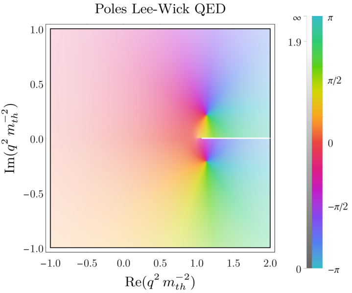
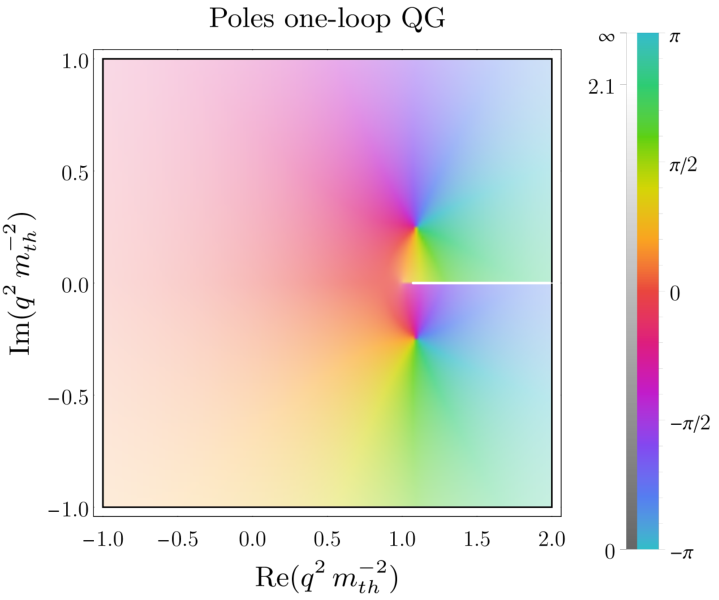
Using the Cauchy integral formula (2.1), the structure of both propagators is
| (72) |
where is the continuum part of the spectral density and is to be positive (for asymptotic states, cf. Sect. 2.4) in order to preserve unitarity. Its specific form determines the physical interpretation of the branch cut, i.e., whether it describes a resonance or a multi-particle state.
The physical sheet of the complex plane is defined by applying the Feynman prescription . The latter plays a key role in determining the sign of the imaginary part of the self-energy. Only after computations one can safely take the limit . Restricting to and applying the Feynman prescription to the propagator yields
| (73) |
Note that if one does not use the Feynman prescription, the imaginary part of the logarithm on the real axis comes with an opposite sign. The above equation, which holds for , justifies the expression (19), where the imaginary part of the logarithm is approximated by a Heaviside step function. Let us remark however that this approximation is only reliable close to the real axis, while in general the complex logarithm should be treated as in the previous two subsections.
All in all, when evaluated on the real axis, the -functions read
| (74) |
These are the expressions to be used to determine the contribution of the branch cut region to the scalar part of the propagator, i.e., to evaluate the integral in Eq. (72). The functions and have no real zeros. On the other hand, the existence of zeros at for the real part of (cf. Fig. 16) tells us that in both cases there is an unstable degree of freedom, specifically, a ghost. Unitarity thus crucially depends on the positivity of . In turn, this is determined by the propagator along the cut


| (75) |
Here can be written as
| (76) |
where is a constant, is the self-energy contribution to the propagator and the (real) solution of defines the mass of the resonance (if there is no real solution, the cut describes a multi-particle state). For instance, in the case of Lee-Wick QED, the real part of the inverse propagator has a real zero, and
| (77) |
so that . Therefore, in this case the imaginary part of the self-energy is small and negative (the same holds true in one-loop QG) and, additionally, it is constant along the cut.
If the cut describes a resonance of mass and if the interaction coupling that makes this degree of freedom unstable is small, (as in the case of one-loop QG and Lee-Wick QED, where ), one can approximate
| (78) |
where the decay width is given by and is defined as
| (79) |
The corresponding spectral density is thus approximated by a Breit-Wigner distribution
| (80) |
For an unstable ghost the constant is negative and thus unitarity requires the decay width to be negative. As we already mentioned, this is the case in Lee-Wick QED and also in one-loop QG Donoghue:2019ecz; Donoghue:2019fcb. However, due to the negative decay width, the pole corresponding to the unstable ghost lies on the first (physical) Riemann sheet Donoghue:2019ecz; Donoghue:2019fcb1212 12 This is to be contrasted with the case of standard resonances, which come with positive width and appear in the second Riemann sheet only.. As detailed in Sect. 4, preserving unitarity in this case comes at the expense of vacuum instabilities and a violation of causality on time scales . In addition, the presence of the complex-conjugate poles in the -complex plane, beyond bringing additional acausalities, makes it impossible to Wick-rotate. In order to perform an analytical continuation, one would need to resort to modified integration contours, such as those determined by the Lee-Wick (LW) Lee:1971ix or Cutkosky-Landshoff-Olive-Polkinghorne (CLOP) prescriptions Cutkosky:1969fq, to translate the Lorentzian description into the Euclidean one (and vice versa).
Summarizing, due to the complex conjugate root theorem, logarithmic quantum corrections to bare higher-derivative theories typically yield dressed propagators displaying additional real (possibly tachyonic and ghost-like) poles or complex-conjugate poles. In the former case, one would loose unitarity (possibly gaining tachyonic instabilities), in the latter the theory would be prone to acausalities (and eventually to vacuum instabilities) and it would not be possible to perform an analytic Wick rotation. In both cases, the unstable ghost associated with the branch cut would lead to acausalities.
Nonetheless, one-loop corrections are not the end of the story. Resumming all quantum fluctuations is expected to result in non-local effective actions with more elaborate form factors. In the next section we will discuss some examples of propagators that are free from additional poles and for which an analytic continuation can be performed.
In accordance with the literature, logarithmic quantum corrections to higher-derivative theories can generally add complex-conjugate poles, tachyonic degrees of freedom and unstable ghosts. Thus, preserving causality and unitarity while avoiding instabilities requires more sophisticated non-local quantum corrections, beyond the one-loop approximation.
6 Consistent graviton propagators: some examples
The integration of quantum gravitational fluctuations (or, more generally, massless fields) at the level of the path integral is expected to yield a non-local effective action. In the one-loop approximation, the form factors are logarithmic. As we discussed in the previous section, logarithmic form factors are enough to make the theory unitary but typically introduce acausalities and instabilities. This suggest that the coexistence of unitarity, causality and stability in theories whose bare action has higher derivatives requires resumming all quantum effects into a more sophisticated non-local effective action.
In this section we discuss and compare two examples of propagators–that proposed in Platania:2020knd and the one derived in Wetterich:2020cxq; Wetterich:2021ywr; Wetterich:2021hru–compatible with all requirements of causality, unitarity and stability discussed throughout the manuscript, including the possibility to perform an analytic Wick rotation. We shall see that a common feature of these propagators is the presence of two symmetric branch cuts. However, for the propagator in Wetterich:2020cxq; Wetterich:2021ywr; Wetterich:2021hru performing an analytic Wick rotation may require a specific prescription for the choice of location of branch cuts. Finally, we will discuss and compare three classes of propagators which might play a role in some approaches to QG (see also Knorr:2021iwv), and which could implement a certain form of dimensional reduction Carlip:2017eud.
6.1 Wetterich propagators
In QFT, unitarity requires that no ghosts (at least, no stable ghosts) appear in the physical spectrum of the theory. In the case of non-gauge theories, this is equivalent to saying that the dressed propagator should not display additional real poles beyond the massless one (cf. Sect. 2). Causality and (vacuum) stability further restrict the pole structure of the propagator: no complex poles should be located in the first or third quadrant of the physical Riemann sheet of the -complex energy plane1313 13 Standard (i.e., non-ghost) unstable particles are typically described by complex poles lying in the first quadrant of the complex energy plane. However, since their decay width is positive, the corresponding poles are located on the second Riemann sheet. Wick rotation is thereby not forbidden by the presence of this type of complex poles. (cf. Sect. 4). Analytic continuation additionally requires the absence of essential singularities.
A propagator satisfying all these requirements has been proposed in Platania:2020knd. Its scalar part in Lorentzian signature reads
| (81) |
where is a mass scale. As detailed in Platania:2020knd, this propagator is endowed with two branch cut singularities along the real axis. If no additional poles exist beyond the massless one (cf. Fig. 17 and Fig. 18). Since the real part of the inverse propagator is always positive, the branch cut singularities do not describe an unstable (ghost) degree of freedom, but rather two symmetric multi-particle states. The spectral density is positive-definite for , thus no violation of unitarity is expected in this case. Moreover, as shown in Fig. 18, for there are no complex poles and thus, based on the arguments we discussed in Sect. 4, no violation of causality ought to occur. Finally, the absence of complex poles in the first and third quadrants of the -complex plane, together with the absence of singularities at infinity, make it possible to connect the Euclidean and Lorentzian versions of the theory via an analytic Wick rotation.


Let us now discuss the graviton propagator derived in Wetterich:2020cxq; Wetterich:2021ywr; Wetterich:2021hru and compare it with the one proposed in Platania:2020knd and reviewed above. The scalar part of the propagator derived in Wetterich:2020cxq; Wetterich:2021ywr; Wetterich:2021hru reads
| (82) |
where in the Lorentzian and in the Euclidean signature, , and is a parameter. In the following we will use the dimensionless momentum square with . In order to have a massless pole, one has to require . One additional ghost pole at appears under the signature-independent condition
| (83) |
In what follows, we shall restrict ourselves to the case and . Due to the presence of the square root, there are branch cuts in the complex energy plane. The branch points are
| (84) |
and they are located along the positive real axis if . In contrast, in Euclidean signature they would be located along the negative real axis. Finally, independent of the signature, for the branch points are complex conjugates and two branch cuts appear parallel to the imaginary axis. It is also important to notice that if , so that one can distinguish three cases:
- •
: The branch points are complex conjugates and two branch cuts appear parallel to the imaginary axis. There are no additional ghost poles and the spectral density is positive.
- •
: Branch cuts appear along the real -axis, and the inverse propagator develops an imaginary part (the spectral density thus has a continuum part, corresponding to a multi-particle state). In this case there are no additional ghost poles and Wick rotation is straighforward, as in Platania:2020knd; however, for any in this range, the -function develops an imaginary part along where the spectral density becomes negative.
- •
: In this case there are multi-particle states with negative spectral density and additional ghost poles. Unitarity is thus violated.
The spectral density associated with these three cases is depicted in Fig. 19 for the case and (in Planck units), while Fig. 20 compares the propagators in Eqs (81) and (82).


Ghosts and a negative spectral density are avoided for . In the next subsection we will explain how to perform an analytic continuation in this case.
6.1.1 Digression: Wick rotation via Sommerfeld branch cuts
We now focus on the possibility of performing an analytical Wick rotation in the presence of branch cuts that are parallel to the imaginary axis. To this end, we note that in the -plane, if there are four symmetric branch points along the real axis in Lorentzian, and along the imaginary axis in Euclidean signature. If instead , the two branch points on the -plane translate in two pairs of complex-conjugate branch points in the -complex plane, independently of the signature. Thus, in all these cases, the branch cuts of the propagator (82) cross all quadrants of the complex energy plane. Wick rotation thus cannot be performed, at least not straightforwardly. In particular, since the branch cuts are a continuum of singular points, one cannot use a modified contour à la Lee-Wick to circumvent the problem. On the other hand, since the location of the branch cuts depends on the convention on the domain of the principal argument, one can change the location of the branch cuts while keeping the location of the branch points fixed. In this procedure one has to make sure not to alter the values of the -function along the real axis, since the reality of the -function along the real axis is related to the stability properties of the given degrees of freedom. We thus use the replacement rule
| (85) |
with . Specifically, the choice corresponds to the conventional case where , while the choice reproduces in this case the Sommerfeld (hyperbolic) branch cut. Examples of this implementation are shown in Fig. 21 for the case of one and two branch points and cuts.


In our case, the branch points are located in all quadrants in the -complex plane and, as depicted in Fig. 22, after rotating the branch cuts, one ends up with four “hooks” connecting the four branch points with and . Next, by employing the -prescription, the branch points can be moved towards the second and fourth quadrant of the complex energy plane. Therefore, combining an appropriate rotation of the branch cuts with the Feynman -prescription one can remove them from the first and third quadrants (cf. Fig. 22), thereby allowing for an analytic Wick rotation.


6.2 Propagators mimicking dimensional reduction versus exponential form factors
In the last subsection we examined two propagators satisfying all properties required by unitarity, stability, and causality that we discussed throughout the manuscript. Despite their nice features in this regard, these propagators cannot be compatible with a well-defined UV completion in terms of an UV fixed point of the RG flow. The latter would indeed require a certain form of effective dimensional reduction Carlip:2017eud.
In this final subsection we shall compare the features of the propagators stemming from three different effective actions or derivations. We will work here with dimensionless momenta for shortness. Chronologically, the first is
| (86) |
and it comes from the simplest non-local gravity model Tomboulis:1997gg; Modesto:2011kw; Biswas:2011ar; Tomboulis:2015esa. As a caveat, within non-local gravity the exponential form factor is assumed to arise at the level of the bare action1414 14 Note that despite its interpretation as a bare action, the corresponding action is not derived from first-principle computations, e.g., as an RG fixed point of some theory. Moreover, since the bare action is non-local, these theories violate locality at a fundamental level., and it is not clear whether its form is preserved along the RG flow, since there is no known symmetry or mechanism preventing other non-exponential operators from being generated by quantum fluctuations. This also means that some properties that seem to be satisfied at a perturbative level w.r.t. the bare action could be spoiled by quantum fluctuations (see, e.g., Shapiro:2015uxa for an example of this mechanism). To allow for a consistent comparison with the other propagators we will introduce, we shall assume that quantum fluctuations indeed preserve the structure of this exponential form factor at quadratic order, and we shall thus re-interpret as (the scalar part of) a dressed propagator. The second propagator we will consider is
| (87) |
and comes from the effective action proposed in Draper:2020bop. The motivation behind the proposal was to provide a proof of principle that effective actions can exist, that are compatible with positivity and causality bounds (at the level of scattering amplitudes), as well as with Weinberg’s asymptotic safety condition. Finally, we will analyze the properties of the dressed graviton propagator numerically-derived in Fehre:2021eob using a spectral version of the FRG Braun:2022mgx which also accounts for Lorentzian signature. The spectral density in this case is analytically approximated by the interpolating function
| (88) |
and the corresponding scalar part of the propagator for the transverse-traceless is given by
| (89) |
Note that in the expression above the -prescription is crucial to avoid unphysical singularities at timelike momenta.
In what follows we shall compare these three propagators and some of their properties. See also Knorr:2021iwv for a complementary comparison of the first two form factors. For a given propagator , a momentum-dependent version of the anomalous dimension may be implicitly defined by
| (90) |
Nonetheless, this map between and is not bijective in and therefore a naïve inversion of this formula can result in unphysical divergences of at finite momentum. A definition avoiding this issue is
| (91) |
and we will employ the latter to determine the anomalous dimension associated with each .
The properties of the three propagators are depicted in Fig. 23, which shows their pole structure (top panel) and the momentum-dependent anomalous dimension (bottom panel).


Focusing on the propagator , the absence of additional poles beyond the massless one indicates that causality and perturbative unitarity are preserved at the level of the two-point function. Nonetheless, the presence of essential singularities at infinity forbids performing an analytic Wick rotation (this problem could be alleviated employing a different prescription for the analytic continuation Buoninfante:2022krn) and makes it difficult to generalize some results in QFT whose derivation makes use of the Cauchy integral formula1515 15 See Pius:2016jsl for first steps towards overcoming this issue.. A final important observation is that the momentum-dependent anomalous dimension diverges to minus infinity in the limit , potentially indicating that this type of exponential form factors might not be compatible with a standard UV completion defined by an RG fixed-point action. This is compatible with the findings in Fraaije:2022uhg: UV non-locality requires the presence of fundamental scales in the fixed-point effective action, but such mass or length scales would explicitly break the scale invariance required for the theory to be UV-completed by a standard RG fixed point.
The behavior of the anomalous dimensions and is instead qualitatively similar. The function varies continuously in the range , being the limiting value for large momenta, and thus entails an effective dimensional reduction Carlip:2017eud from four (small momenta) to two (large momenta) spacetime dimensions. The anomalous dimension instead varies in the range , and approaches the value as . Both behaviors are compatible with the existence of a non-trivial fixed point in the UV Christiansen:2014raa; Draper:2020bop; Fehre:2021eob. Despite these similarities, the propagators and have a very different pole structure: aside from the massless pole located at the origin of the -complex plane, the former is characterized by an infinite number of massless complex-conjugate poles, while the latter does not have any additional poles and only displays a branch cut singularity for . The tower of massless complex-conjugate poles characterizing is key to satisfy both causality bounds and Weinberg’s asymptotic safety condition in Draper:2020bop. Yet, according to the discussion in Sect. 4, such complex-conjugate pairs entail a violation of causality in terms of backward propagation of modes with positive energy (similarly to Lee-Wick theories) and vacuum instabilities as defined in the same section (unless a stabilizing mechanism exists1616 16 The question of whether a stabilizing mechanism exists in general is insofar unexplored. It is worth mentioning that the case of Draper:2020bop should be explored separately, since the interplay of infinitely many complex-conjugate poles might give rise to non-trivial effects, and could differ from the case of a single pair of complex-conjugate poles.). The branch cut in is instead expected, since at low energies one should recover the one-loop logarithmic corrections to the classical action (cf. Sect. 5). Together with the absence of complex poles, this makes fully consistent w.r.t. all properties discussed throughout this manuscript and with standard EFT results. At the same time, it is an open question whether scattering amplitudes determined using the techniques in Fehre:2021eob will display the same desirable properties as those stemming from the form factors studied in Draper:2020bop.
7 Discussion and conclusions
The perturbative quantization of General Relativity yields a theory that is perturbatively non-renormalizable but unitary. Adding a finite number of higher derivatives improves the ultraviolet behavior of gravity, but introduces ghosts.
In an attempt to reconcile renormalizability and unitarity, many theories of quantum gravity have been advanced. Yet, independent of the specific ultraviolet completion of gravity, it is a key question what the properties of the dressed graviton propagator should be, at least ideally, and whether there exist propagators satisfying all these properties. Motivated by these questions, in this work we have discussed various aspects of causality, unitarity and stability, and their implications for the properties of the dressed (graviton) propagator.
First, we argued that unitarity of quantum field theories is best understood at the level of the effective action, and that truncations of the latter based on both entire and non-entire form factors lead to the appearance of fictitious ghosts. In particular, we provided numerical evidence (see. Sect. 3) for the residue decoupling mechanism of fictitious ghosts theorized in Platania:2020knd. Second, we collected various inequivalent notions and definitions of causality that appear in the literature, and we discussed their relations. We also provided a detailed analysis of ghost and tachyonic instabilities, at the classical and quantum level, showing that at the quantum level tachyonic instabilities can be less severe than the vacuum instabilities provoked by unstable degrees of freedom with negative width and complex-conjugate poles. In this course, we highlighted a key difference between quantum ghost and tachyonic instabilities: the former is a “kinetic problem”, and its resolutions in a non-perturbative setup is to be sought in the momentum dependence of the effective action. The latter is a “potential problem” and its resolution lies in the field dependence of the effective action. An explicit example of how interaction terms in the effective action can cure tachyonic instabilities was provided in Sect. 4.2.3. The relation between poles of a dressed propagator, and some forms of causality, unitarity and stability is summarized in Tab. 2. An exact formula quantifying the causality violation is derived in Sect. 4.3, cf. Eq. (51), and is depicted in Fig. 11. Third, we showed that logarithmic corrections to the classical action are not sufficient to ameliorate the behavior of the theory, as the corresponding propagator displays either complex-conjugate poles (implying a violation of causality and vacuum instabilities) or stable tachyonic ghosts (implying a violation of unitarity, as well as tachyonic instabilities). Accounting for the infinitely many derivatives at the level of the effective action is crucial, but not sufficient. Thus, we discussed and compared some examples of consistent field theories whose dynamics—encoded in the quantum effective action—preserves causality, (vacuum and tachyonic) stability and unitarity at the level of the two-point function, and whose Euclidean theory is connected to the Lorentzian one via an analytical Wick rotation. In particular, the propagator computed in Fehre:2021eob seems ideal in this respect, it being compatible with all properties listed and analyzed here, as well as with Weinberg’s asymptotic safety condition. Our work thus provides further support to the possibility of formulating a consistent and stable quantum theory of gravity compatible with all fundamental principles of quantum field theory.
Acknowledgements
The author thanks D. Anselmi, I. Basile, L. Buoninfante, J. Donoghue, A. Eichhorn, B. Knorr, R. Percacci, A. Pereira, M. Reichert and C. Wetterich for many insightful discussions. The author is also grateful to M. Reichert for providing the interpolating function in Eq. (88) and to B. Knorr for very helpful comments on the manuscript. During part of the development of this work, A.P. was supported by the Alexander von Humboldt Foundation. A.P. acknowledges support by Perimeter Institute for Theoretical Physics. Research at Perimeter Institute is supported in part by the Government of Canada through the Department of Innovation, Science and Economic Development Canada and by the Province of Ontario through the Ministry of Colleges and Universities.
References
- (1) G. ’t Hooft and M. J. G. Veltman, One loop divergencies in the theory of gravitation, Ann. Inst. H. Poincare Phys. Theor. A 20 (1974) 69.
- (2) M. H. Goroff and A. Sagnotti, Quantum gravity at two loops, Physics Letters B 160 (1985) 81.
- (3) M. H. Goroff and A. Sagnotti, The ultraviolet behavior of Einstein gravity, Nuclear Physics B 266 (1986) 709.
- (4) A. E. M. van de Ven, Two loop quantum gravity, Nucl. Phys. B 378 (1992) 309.
- (5) K. S. Stelle, Classical Gravity with Higher Derivatives, Gen. Rel. Grav. 9 (1978) 353.
- (6) K. G. Wilson and J. B. Kogut, The Renormalization group and the epsilon expansion, Phys. Rept. 12 (1974) 75.
- (7) S. Weinberg, Critical Phenomena for Field Theorists, Erice Subnuclear Physics (1976) .
- (8) S. de Alwis, A. Eichhorn, A. Held, J. M. Pawlowski, M. Schiffer and F. Versteegen, Asymptotic safety, string theory and the weak gravity conjecture, Phys. Lett. B 798 (2019) 134991 [1907.07894].
- (9) I. Basile and A. Platania, Cosmological ’-corrections from the functional renormalization group, JHEP 06 (2021) 045 [2101.02226].
- (10) A. Eichhorn, Status of the asymptotic safety paradigm for quantum gravity and matter, Found. Phys. 48 (2018) 1407 [1709.03696].
- (11) J. F. Donoghue, A Critique of the Asymptotic Safety Program, Front. in Phys. 8 (2020) 56 [1911.02967].
- (12) J. M. Pawlowski and M. Reichert, Quantum Gravity: A Fluctuating Point of View, Front. in Phys. 8 (2021) 551848 [2007.10353].
- (13) A. Bonanno, A. Eichhorn, H. Gies, J. M. Pawlowski, R. Percacci, M. Reuter et al., Critical reflections on asymptotically safe gravity, Front. in Phys. 8 (2020) 269 [2004.06810].
- (14) J. Laiho, S. Bassler, D. Coumbe, D. Du and J. T. Neelakanta, Lattice Quantum Gravity and Asymptotic Safety, ArXiv e-prints (2016) [1604.02745].
- (15) R. Loll, Quantum Gravity from Causal Dynamical Triangulations: A Review, Class. Quant. Grav. 37 (2020) 013002 [1905.08669].
- (16) N. Dupuis, L. Canet, A. Eichhorn, W. Metzner, J. M. Pawlowski, M. Tissier et al., The nonperturbative functional renormalization group and its applications, Phys. Rept. 910 (2021) 1 [2006.04853].
- (17) E. Manrique and M. Reuter, Bare Action and Regularized Functional Integral of Asymptotically Safe Quantum Gravity, Phys. Rev. D 79 (2009) 025008 [0811.3888].
- (18) T. R. Morris and Z. H. Slade, Solutions to the reconstruction problem in asymptotic safety, JHEP 11 (2015) 094 [1507.08657].
- (19) M. Fraaije, A. Platania and F. Saueressig, On the reconstruction problem in Quantum Gravity, 2206.10626.
- (20) W. Souma, Non-Trivial Ultraviolet Fixed Point in Quantum Gravity, Progress of Theoretical Physics 102 (1999) 181 [hep-th/9907027].
- (21) O. Lauscher and M. Reuter, Flow equation of quantum Einstein gravity in a higher-derivative truncation, Phys. Rev. D 66 (2002) 025026 [hep-th/0205062].
- (22) D. F. Litim, Fixed Points of Quantum Gravity, Physical Review Letters 92 (2004) 201301 [hep-th/0312114].
- (23) A. Codello and R. Percacci, Fixed Points of Higher-Derivative Gravity, Physical Review Letters 97 (2006) 221301 [hep-th/0607128].
- (24) P. F. Machado and F. Saueressig, On the renormalization group flow of f(R)-gravity, Phys. Rev. D 77 (2008) 124045 [arXiv:0712.0445].
- (25) D. Benedetti, P. F. Machado and F. Saueressig, Asymptotic Safety in Higher-Derivative Gravity, Modern Physics Letters A 24 (2009) 2233 [0901.2984].
- (26) E. Manrique, S. Rechenberger and F. Saueressig, Asymptotically Safe Lorentzian Gravity, Physical Review Letters 106 (2011) 251302 [1102.5012].
- (27) J. A. Dietz and T. R. Morris, Asymptotic safety in the f(R) approximation, Journal of High Energy Physics 1 (2013) 108 [1211.0955].
- (28) N. Ohta and R. Percacci, Higher Derivative Gravity and Asymptotic Safety in Diverse Dimensions, Class. Quant. Grav. 31 (2014) 015024 [1308.3398].
- (29) P. Donà, A. Eichhorn and R. Percacci, Matter matters in asymptotically safe quantum gravity, Phys. Rev. D 89 (2014) 084035 [1311.2898].
- (30) A. Codello, G. D’Odorico and C. Pagani, Consistent closure of renormalization group flow equations in quantum gravity, Phys. Rev. D 89 (2014) 081701 [1304.4777].
- (31) N. Christiansen, B. Knorr, J. M. Pawlowski and A. Rodigast, Global Flows in Quantum Gravity, Phys. Rev. D93 (2016) 044036 [1403.1232].
- (32) K. Falls, D. Litim, K. Nikolakopoulos and C. Rahmede, Further evidence for asymptotic safety of quantum gravity, Phys. Rev. D 93 (2016) 104022.
- (33) D. Becker and M. Reuter, En route to Background Independence: Broken split-symmetry, and how to restore it with bi-metric average actions, Annals Phys. 350 (2014) 225 [1404.4537].
- (34) N. Christiansen, B. Knorr, J. Meibohm, J. M. Pawlowski and M. Reichert, Local Quantum Gravity, Phys. Rev. D92 (2015) 121501 [1506.07016].
- (35) J. Meibohm, J. M. Pawlowski and M. Reichert, Asymptotic safety of gravity-matter systems, Phys. Rev. D 93 (2016) 084035 [1510.07018].
- (36) K. Y. Oda and M. Yamada, Non-minimal coupling in Higgs-Yukawa model with asymptotically safe gravity, Classical and Quantum Gravity 33 (2016) 125011 [1510.03734].
- (37) J. Biemans, A. Platania and F. Saueressig, Quantum gravity on foliated spacetimes: Asymptotically safe and sound, Phys. Rev. D95 (2017) 086013 [1609.04813].
- (38) A. Eichhorn, A. Held and J. M. Pawlowski, Quantum-gravity effects on a Higgs-Yukawa model, Phys. Rev. D 94 (2016) 104027 [1604.02041].
- (39) K. Falls and N. Ohta, Renormalization group equation for f(R) gravity on hyperbolic spaces, Phys. Rev. D 94 (2016) 084005 [1607.08460].
- (40) H. Gies, B. Knorr, S. Lippoldt and F. Saueressig, Gravitational Two-Loop Counterterm Is Asymptotically Safe, Physical Review Letters 116 (2016) 211302 [1601.01800].
- (41) J. Biemans, A. Platania and F. Saueressig, Renormalization group fixed points of foliated gravity-matter systems, JHEP 05 (2017) 093 [1702.06539].
- (42) N. Christiansen, D. F. Litim, J. M. Pawlowski and M. Reichert, Asymptotic safety of gravity with matter, Phys. Rev. D97 (2018) 106012 [1710.04669].
- (43) Y. Hamada and M. Yamada, Asymptotic safety of higher derivative quantum gravity non-minimally coupled with a matter system, JHEP 08 (2017) 070 [1703.09033].
- (44) A. Platania and F. Saueressig, Functional Renormalization Group Flows on Friedman–Lemaître–Robertson–Walker backgrounds, Found. Phys. 48 (2018) 1291 [1710.01972].
- (45) K. Falls, C. R. King, D. F. Litim, K. Nikolakopoulos and C. Rahmede, Asymptotic safety of quantum gravity beyond Ricci scalars, Phys. Rev. D97 (2018) 086006 [1801.00162].
- (46) A. Eichhorn, S. Lippoldt and M. Schiffer, Zooming in on fermions and quantum gravity, Phys. Rev. D99 (2019) 086002 [1812.08782].
- (47) A. Eichhorn and M. Schiffer, as the critical dimensionality of asymptotically safe interactions, Phys. Lett. B793 (2019) 383 [1902.06479].
- (48) B. Knorr, The derivative expansion in asymptotically safe quantum gravity: general setup and quartic order, SciPost Phys. Core 4 (2021) 020 [2104.11336].
- (49) A. Baldazzi and K. Falls, Essential Quantum Einstein Gravity, Universe 7 (2021) 294 [2107.00671].
- (50) A. Bonanno, T. Denz, J. M. Pawlowski and M. Reichert, Reconstructing the graviton, SciPost Phys. 12 (2022) 001 [2102.02217].
- (51) J. Fehre, D. F. Litim, J. M. Pawlowski and M. Reichert, Lorentzian quantum gravity and the graviton spectral function, 2111.13232.
- (52) B. Knorr, Safe essential scalar-tensor theories, 2204.08564.
- (53) A. Eichhorn, On unimodular quantum gravity, Class. Quant. Grav. 30 (2013) 115016 [1301.0879].
- (54) G. P. De Brito, A. Eichhorn and A. D. Pereira, A link that matters: Towards phenomenological tests of unimodular asymptotic safety, JHEP 09 (2019) 100 [1907.11173].
- (55) G. P. de Brito and A. D. Pereira, Unimodular quantum gravity: Steps beyond perturbation theory, JHEP 09 (2020) 196 [2007.05589].
- (56) G. P. de Brito, A. D. Pereira and A. F. Vieira, Exploring new corners of asymptotically safe unimodular quantum gravity, Phys. Rev. D 103 (2021) 104023 [2012.08904].
- (57) A. Contillo, S. Rechenberger and F. Saueressig, Renormalization group flow of Hořava-Lifshitz gravity at low energies, JHEP 12 (2013) 017 [1309.7273].
- (58) G. D’Odorico, J.-W. Goossens and F. Saueressig, Covariant computation of effective actions in Hořava-Lifshitz gravity, JHEP 10 (2015) 126 [1508.00590].
- (59) B. Knorr, Lorentz symmetry is relevant, Phys. Lett. B792 (2019) 142 [1810.07971].
- (60) A. Eichhorn, A. Platania and M. Schiffer, Lorentz invariance violations in the interplay of quantum gravity with matter, Phys. Rev. D 102 (2020) 026007 [1911.10066].
- (61) A. Eichhorn and T. Koslowski, Continuum limit in matrix models for quantum gravity from the Functional Renormalization Group, Phys. Rev. D 88 (2013) 084016 [1309.1690].
- (62) A. Eichhorn and T. Koslowski, Flowing to the continuum in discrete tensor models for quantum gravity, Ann. Inst. H. Poincare Comb. Phys. Interact. 5 (2018) 173 [1701.03029].
- (63) A. Eichhorn, T. Koslowski and A. D. Pereira, Status of background-independent coarse-graining in tensor models for quantum gravity, Universe 5 (2019) 53 [1811.12909].
- (64) A. Eichhorn, J. Lumma, A. D. Pereira and A. Sikandar, Universal critical behavior in tensor models for four-dimensional quantum gravity, JHEP 02 (2020) 110 [1912.05314].
- (65) D. Benedetti and V. Lahoche, Functional Renormalization Group Approach for Tensorial Group Field Theory: A Rank-6 Model with Closure Constraint, Class. Quant. Grav. 33 (2016) 095003 [1508.06384].
- (66) J. Ben Geloun, R. Martini and D. Oriti, Functional Renormalisation Group analysis of Tensorial Group Field Theories on , Phys. Rev. D 94 (2016) 024017 [1601.08211].
- (67) J. Ben Geloun, T. A. Koslowski, D. Oriti and A. D. Pereira, Functional Renormalization Group analysis of rank 3 tensorial group field theory: The full quartic invariant truncation, Phys. Rev. D 97 (2018) 126018 [1805.01619].
- (68) V. Lahoche and D. O. Samary, Progress in the solving nonperturbative renormalization group for tensorial group field theory, Universe 5 (2019) 86 [1812.00905].
- (69) A. G. A. Pithis and J. Thürigen, Phase transitions in TGFT: functional renormalization group in the cyclic-melonic potential approximation and equivalence to O models, JHEP 12 (2020) 159 [2009.13588].
- (70) I. Basile and A. Platania, String tension between de Sitter vacua and curvature corrections, Phys. Rev. D 104 (2021) L121901 [2103.06276].
- (71) I. Basile and A. Platania, Asymptotic Safety: Swampland or Wonderland?, Universe 7 (2021) 389 [2107.06897].
- (72) F. Gao and M. Yamada, Determining holographic wave functions from Wilsonian renormalization group, 2202.13699.
- (73) R. Ferrero and M. Reuter, AdS/CFT and dS/CFT correspondences emerging from Asymptotic Safety ?, 2205.12030.
- (74) A. Codello, R. Percacci, L. Rachwał and A. Tonero, Computing the Effective Action with the Functional Renormalization Group, Eur. Phys. J. C 76 (2016) 226 [1505.03119].
- (75) B. Knorr and F. Saueressig, Towards reconstructing the quantum effective action of gravity, Phys. Rev. Lett. 121 (2018) 161304 [1804.03846].
- (76) B. Knorr, C. Ripken and F. Saueressig, Form Factors in Asymptotic Safety: conceptual ideas and computational toolbox, Class. Quant. Grav. 36 (2019) 234001 [1907.02903].
- (77) N. Ohta and L. Rachwal, Effective action from the functional renormalization group, Eur. Phys. J. C 80 (2020) 877 [2002.10839].
- (78) B. Knorr and M. Schiffer, Non-Perturbative Propagators in Quantum Gravity, Universe 7 (2021) 216 [2105.04566].
- (79) A. Bonanno and M. Reuter, Spacetime structure of an evaporating black hole in quantum gravity, Phys. Rev. D73 (2006) 083005 [hep-th/0602159].
- (80) K. Falls and D. F. Litim, Black hole thermodynamics under the microscope, Phys. Rev. D89 (2014) 084002 [1212.1821].
- (81) R. Torres and F. Fayos, On the quantum corrected gravitational collapse, Physics Letters B 747 (2015) 245 [1503.07407].
- (82) B. Koch and P. Rioseco, Black Hole Solutions for Scale Dependent Couplings: The de Sitter and the Reissner-Nordström Case, Class. Quant. Grav. 33 (2016) 035002 [1501.00904].
- (83) A. Bonanno and A. Platania, Asymptotically safe inflation from quadratic gravity, Phys. Lett. B750 (2015) 638 [1507.03375].
- (84) A. Bonanno and A. Platania, Asymptotically Safe R+R2 gravity, PoS corfu2015 (2016) 159.
- (85) G. Kofinas and V. Zarikas, Asymptotically Safe gravity and non-singular inflationary Big Bang with vacuum birth, Phys. Rev. D94 (2016) 103514 [1605.02241].
- (86) K. Falls, D. F. Litim, K. Nikolakopoulos and C. Rahmede, On de Sitter solutions in asymptotically safe theories, Class. Quant. Grav. 35 (2018) 135006 [1607.04962].
- (87) A. Bonanno, B. Koch and A. Platania, Cosmic Censorship in Quantum Einstein Gravity, Class. Quant. Grav. 34 (2017) 095012 [1610.05299].
- (88) A. Bonanno, S. J. Gabriele Gionti and A. Platania, Bouncing and emergent cosmologies from Arnowitt-Deser-Misner RG flows, Class. Quant. Grav. 35 (2018) 065004 [1710.06317].
- (89) A. Bonanno, B. Koch and A. Platania, Asymptotically Safe gravitational collapse: Kuroda-Papapetrou RG-improved model, PoS corfu2016 (2017) 058.
- (90) A. Bonanno, B. Koch and A. Platania, Gravitational collapse in Quantum Einstein Gravity, Found. Phys. 48 (2018) 1393 [1710.10845].
- (91) A. Bonanno, A. Platania and F. Saueressig, Cosmological bounds on the field content of asymptotically safe gravity–matter models, Phys. Lett. B 784 (2018) 229 [1803.02355].
- (92) L.-H. Liu, T. Prokopec and A. A. Starobinsky, Inflation in an effective gravitational model and asymptotic safety, Phys. Rev. D98 (2018) 043505 [1806.05407].
- (93) A. Majhi, Singularity from star collapse, torsion and asymptotic safety of gravity, 1804.00960.
- (94) F. K. Anagnostopoulos, S. Basilakos, G. Kofinas and V. Zarikas, Constraining the Asymptotically Safe Cosmology: cosmic acceleration without dark energy, JCAP 1902 (2019) 053 [1806.10580].
- (95) A. Adeifeoba, A. Eichhorn and A. Platania, Towards conditions for black-hole singularity-resolution in asymptotically safe quantum gravity, Class. Quant. Grav. 35 (2018) 225007 [1808.03472].
- (96) J. M. Pawlowski and D. Stock, Quantum-improved Schwarzschild-(A)dS and Kerr-(A)dS spacetimes, Phys. Rev. D98 (2018) 106008 [1807.10512].
- (97) G. Gubitosi, R. Ooijer, C. Ripken and F. Saueressig, Consistent early and late time cosmology from the RG flow of gravity, JCAP 1812 (2018) 004 [1806.10147].
- (98) A. Platania, The inflationary mechanism in Asymptotically Safe Gravity, Universe 5 (2019) 189 [1908.03897].
- (99) A. Platania, Dynamical renormalization of black-hole spacetimes, Eur. Phys. J. C79 (2019) 470 [1903.10411].
- (100) A. Bonanno, R. Casadio and A. Platania, Gravitational antiscreening in stellar interiors, JCAP 2001 (2020) 022 [1910.11393].
- (101) A. Held, R. Gold and A. Eichhorn, Asymptotic safety casts its shadow, JCAP 1906 (2019) 029 [1904.07133].
- (102) L. Bosma, B. Knorr and F. Saueressig, Resolving Spacetime Singularities within Asymptotic Safety, Phys. Rev. Lett. 123 (2019) 101301 [1904.04845].
- (103) B. Knorr and A. Platania, Sifting quantum black holes through the principle of least action, 2202.01216.
- (104) A. Bonanno and F. Saueressig, Asymptotically safe cosmology - A status report, Comptes Rendus Physique 18 (2017) 254 [1702.04137].
- (105) A. Platania, From renormalization group flows to cosmology, Front. in Phys. 8 (2020) 188 [2003.13656].
- (106) T. Draper, B. Knorr, C. Ripken and F. Saueressig, Finite Quantum Gravity Amplitudes: No Strings Attached, Phys. Rev. Lett. 125 (2020) 181301 [2007.00733].
- (107) T. Draper, B. Knorr, C. Ripken and F. Saueressig, Graviton-Mediated Scattering Amplitudes from the Quantum Effective Action, JHEP 11 (2020) 136 [2007.04396].
- (108) B. Knorr and C. Ripken, Scattering amplitudes in affine gravity, Phys. Rev. D 103 (2021) 105019 [2012.05144].
- (109) R. Ferrero and C. Ripken, De Sitter scattering amplitudes in the Born approximation, 2112.03766.
- (110) B. Knorr, S. Pirlo, C. Ripken and F. Saueressig, Cartographing gravity-mediated scattering amplitudes: scalars and photons, 2205.01738.
- (111) A. Adams, N. Arkani-Hamed, S. Dubovsky, A. Nicolis and R. Rattazzi, Causality, analyticity and an IR obstruction to UV completion, JHEP 10 (2006) 014 [hep-th/0602178].
- (112) C. Cheung and G. N. Remmen, Positive Signs in Massive Gravity, JHEP 04 (2016) 002 [1601.04068].
- (113) B. Bellazzini, Softness and amplitudes’ positivity for spinning particles, JHEP 02 (2017) 034 [1605.06111].
- (114) C. de Rham, S. Melville, A. J. Tolley and S.-Y. Zhou, UV complete me: Positivity Bounds for Particles with Spin, JHEP 03 (2018) 011 [1706.02712].
- (115) C. de Rham, S. Melville and A. J. Tolley, Improved Positivity Bounds and Massive Gravity, JHEP 04 (2018) 083 [1710.09611].
- (116) C. de Rham, S. Melville, A. J. Tolley and S.-Y. Zhou, Positivity Bounds for Massive Spin-1 and Spin-2 Fields, JHEP 03 (2019) 182 [1804.10624].
- (117) C. De Rham, L. Heisenberg and A. J. Tolley, Spin-2 fields and the weak gravity conjecture, Phys. Rev. D 100 (2019) 104033 [1812.01012].
- (118) L. Alberte, C. de Rham, A. Momeni, J. Rumbutis and A. J. Tolley, EFT of Interacting Spin-2 Fields, JHEP 01 (2020) 131 [1910.05285].
- (119) L. Alberte, C. de Rham, A. Momeni, J. Rumbutis and A. J. Tolley, Positivity Constraints on Interacting Spin-2 Fields, JHEP 03 (2020) 097 [1910.11799].
- (120) L. Alberte, C. de Rham, A. Momeni, J. Rumbutis and A. J. Tolley, Positivity Constraints on Interacting Pseudo-Linear Spin-2 Fields, JHEP 07 (2020) 121 [1912.10018].
- (121) L. Alberte, C. de Rham, S. Jaitly and A. J. Tolley, QED positivity bounds, Phys. Rev. D 103 (2021) 125020 [2012.05798].
- (122) L. Alberte, C. de Rham, S. Jaitly and A. J. Tolley, Positivity Bounds and the Massless Spin-2 Pole, Phys. Rev. D 102 (2020) 125023 [2007.12667].
- (123) C. de Rham, S. Melville and J. Noller, Positivity bounds on dark energy: when matter matters, JCAP 08 (2021) 018 [2103.06855].
- (124) M. Herrero-Valea, A. S. Koshelev and A. Tokareva, UV graviton scattering and positivity bounds from IR dispersion relations, 2205.13332.
- (125) C. de Rham, S. Kundu, M. Reece, A. J. Tolley and S.-Y. Zhou, Snowmass White Paper: UV Constraints on IR Physics, in 2022 Snowmass Summer Study, 3, 2022, 2203.06805.
- (126) J. F. Donoghue and G. Menezes, Massive poles in Lee-Wick quantum field theory, Phys. Rev. D99 (2019) 065017 [1812.03603].
- (127) J. F. Donoghue and G. Menezes, Arrow of Causality and Quantum Gravity, Phys. Rev. Lett. 123 (2019) 171601 [1908.04170].
- (128) J. F. Donoghue and G. Menezes, Unitarity, stability and loops of unstable ghosts, Phys. Rev. D100 (2019) 105006 [1908.02416].
- (129) J. F. Donoghue and G. Menezes, Causality and gravity, JHEP 11 (2021) 010 [2106.05912].
- (130) C. Wetterich, Quantum scale symmetry, 1901.04741.
- (131) A. Platania and C. Wetterich, Non-perturbative unitarity and fictitious ghosts in quantum gravity, Phys. Lett. B 811 (2020) 135911 [2009.06637].
- (132) I. Kuntz, Exorcising ghosts in quantum gravity, Eur. Phys. J. Plus 135 (2020) 859 [1909.11072].
- (133) G. Kallen, On the definition of the Renormalization Constants in Quantum Electrodynamics, Helv. Phys. Acta 25 (1952) 417.
- (134) H. Lehmann, On the Properties of propagation functions and renormalization contants of quantized fields, Nuovo Cim. 11 (1954) 342.
- (135) C. Wetterich, Exact evolution equation for the effective potential, Physics Letters B 301 (1993) 90.
- (136) T. R. Morris, The Exact Renormalization Group and Approximate Solutions, International Journal of Modern Physics A 9 (1994) 2411 [hep-ph/9308265].
- (137) M. Reuter and C. Wetterich, Effective average action for gauge theories and exact evolution equations, Nuclear Physics B 417 (1994) 181.
- (138) M. Reuter, Nonperturbative evolution equation for quantum gravity, Phys. Rev. D57 (1998) 971 [hep-th/9605030].
- (139) E. S. Fradkin and A. A. Tseytlin, Asymptotic freedom in renormalizable gravity and supergravity, in Second Seminar on Quantum Gravity Moscow, USSR, October 13-15, 1981, pp. 29–45, 1981.
- (140) M. J. G. Veltman, Unitarity and causality in a renormalizable field theory with unstable particles, Physica 29 (1963) 186.
- (141) Y. Hayashi and K.-I. Kondo, Complex poles and spectral function of Yang-Mills theory, Phys. Rev. D 99 (2019) 074001 [1812.03116].
- (142) K.-I. Kondo, Y. Hayashi, R. Matsudo, Y. Suda and M. Watanabe, Complex poles, spectral function and reflection positivity violation of Yang-Mills theory, PoS LC2019 (2019) 053 [1912.06261].
- (143) A. Bonanno and M. Reuter, Modulated Ground State of Gravity Theories with Stabilized Conformal Factor, Phys. Rev. D87 (2013) 084019 [1302.2928].
- (144) L. D. Landau, A. A. Abrikosov and I. M. Khalatnikov, Asimptoticheskoe vyrazhenie dlia funktsii Grina elektrona v kvantovoi elektrodinamike, Dokl. Akad. Nauk SSSR 95 (1954) 773.
- (145) J. F. Donoghue and B. K. El-Menoufi, Covariant non-local action for massless QED and the curvature expansion, JHEP 10 (2015) 044 [1507.06321].
- (146) J. F. Donoghue and B. K. El-Menoufi, QED trace anomaly, non-local Lagrangians and quantum Equivalence Principle violations, JHEP 05 (2015) 118 [1503.06099].
- (147) D. G. Boulware and D. J. Gross, Lee-Wick indefinite metric quantization: a functional integral approach, Nucl. Phys. B233 (1984) 1.
- (148) A. Platania, On the residue decoupling mechanism of fictitious ghosts, .
- (149) C. de Rham and A. J. Tolley, Causality in curved spacetimes: The speed of light and gravity, Phys. Rev. D 102 (2020) 084048 [2007.01847].
- (150) O. M. P. Bilaniuk, V. K. Deshpande and E. C. G. Sudarshan, Meta Relativity, Am. J. Phys. 30 (1962) 718.
- (151) W. B. Rolnick, Implications of causality for faster-than-light matter, Phys. Rev. 183 (1969) 1105.
- (152) P. L. Csonka, Causality and faster than light particles, Nucl. Phys. B 21 (1970) 436.
- (153) J. Friedman, M. S. Morris, I. D. Novikov, F. Echeverria, G. Klinkhammer, K. S. Thorne et al., Cauchy problem in space-times with closed timelike curves, Phys. Rev. D 42 (1990) 1915.
- (154) D. Deutsch, Quantum mechanics near closed timelike lines, Phys. Rev. D 44 (1991) 3197.
- (155) A. E. Everett, Warp drive and causality, Phys. Rev. D 53 (1996) 7365.
- (156) J. C. Garrison, M. W. Mitchell, R. Y. Chiao and E. L. Bolda, Superluminal signals: Causal loop paradoxes revisited, Phys. Lett. A 245 (1998) 19 [quant-ph/9810031].
- (157) M. Gell-Mann, M. L. Goldberger and W. E. Thirring, Use of causality conditions in quantum theory, Phys. Rev. 95 (1954) 1612.
- (158) Y. Aharonov, A. Komar and L. Susskind, Superluminal behavior, causality, and instability, Phys. Rev. 182 (1969) 1400.
- (159) N. N. Bogoljubow and D. W. Schirkow, Probleme der quantentheorie der felder, Fortschritte der Physik 3 (1955) 439 [https://onlinelibrary.wiley.com/doi/pdf/10.1002/prop.19550030903].
- (160) N. N. Bogoljubow, D. W. Schirkow and H. Vogel, Probleme der quantenfeldtheorie) ii. beseitigung der divergenzen aus der streumatrix), Fortschritte der Physik 4 (1956) 438 [https://onlinelibrary.wiley.com/doi/pdf/10.1002/prop.19560040903].
- (161) G. V. Efimov, Non-local quantum theory of the scalar field, Commun. Math. Phys. 5 (1967) 42.
- (162) F. A. Cerulus and A. Martin, A lower bound for large-angle elastic scattering at high energies, Phys. Lett. 8 (1964) 80.
- (163) S. B. Giddings, The gravitational S-matrix: Erice lectures, Subnucl. Ser. 48 (2013) 93 [1105.2036].
- (164) H. Epstein and A. Martin, Rigorous lower bound on the scattering amplitude at large angles, Phys. Rev. D 99 (2019) 114025 [1903.00953].
- (165) S. Weinberg, The Quantum theory of fields. Vol. 1: Foundations. Cambridge University Press, 6, 2005.
- (166) J. M. Cline, S. Jeon and G. D. Moore, The Phantom menaced: Constraints on low-energy effective ghosts, Phys. Rev. D70 (2004) 043543 [hep-ph/0311312].
- (167) B. Grinstein, D. O’Connell and M. B. Wise, Causality as an emergent macroscopic phenomenon: The Lee-Wick O(N) model, Phys. Rev. D 79 (2009) 105019 [0805.2156].
- (168) U. Habel, R. Konning, H. G. Reusch, M. Stingl and S. Wigard, A Nonperturbative Solution to the Dyson-schwinger Equations of Quantum Chromodynamics. 1. General Properties, Z. Phys. A 336 (1990) 423.
- (169) R. Alkofer and L. von Smekal, The Infrared behavior of QCD Green’s functions: Confinement dynamical symmetry breaking, and hadrons as relativistic bound states, Phys. Rept. 353 (2001) 281 [hep-ph/0007355].
- (170) S. Coleman, Acausality, in 7th International School of Subnuclear Physics (Ettore Majorana): Subnuclear Phenomena, pp. 282–327, 1969.
- (171) R. Cutkosky, P. Landshoff, D. I. Olive and J. Polkinghorne, A non-analytic S matrix, Nucl. Phys. B 12 (1969) 281.
- (172) T. Lee and G. Wick, Questions of Lorentz Invariance in Field Theories With Indefinite Metric, Phys. Rev. D 3 (1971) 1046.
- (173) A. van Tonder, Unitarity, Lorentz invariance and causality in Lee-Wick theories: An asymptotically safe completion of QED, tech. rep., Oct, 2008.
- (174) E. Alvarez, L. Da Rold, C. Schat and A. Szynkman, Vertex Displacements for Acausal Particles: Testing the Lee-Wick Standard Model at the LHC, JHEP 10 (2009) 023 [0908.2446].
- (175) T. G. Rizzo, Searching for Lee-Wick gauge bosons at the LHC, JHEP 06 (2007) 070 [0704.3458].
- (176) T. G. Rizzo, Unique Identification of Lee-Wick Gauge Bosons at Linear Colliders, JHEP 01 (2008) 042 [0712.1791].
- (177) Y. Hayashi and K.-I. Kondo, Reconstructing confined particles with complex singularities, Phys. Rev. D 103 (2021) L111504 [2103.14322].
- (178) L. Baulieu, D. Dudal, M. Guimaraes, M. Huber, S. Sorella, N. Vandersickel et al., Gribov horizon and i-particles: About a toy model and the construction of physical operators, Phys. Rev. D 82 (2010) 025021 [0912.5153].
- (179) D. Binosi and R.-A. Tripolt, Spectral functions of confined particles, Phys. Lett. B 801 (2020) 135171 [1904.08172].
- (180) C. de Rham, A. J. Tolley and J. Zhang, Causality Constraints on Gravitational Effective Field Theories, Phys. Rev. Lett. 128 (2022) 131102 [2112.05054].
- (181) G. Feinberg, Possibility of Faster-Than-Light Particles, Phys. Rev. 159 (1967) 1089.
- (182) R. G. Cawley, Classical charged tachyon selfenergy problem, Phys. Rev. D 2 (1970) 276.
- (183) E. Recami, Tachyon Kinematics and Causality: A Systematic, Thorough Analysis, Found. Phys. 17 (1987) 239.
- (184) V. F. Perepelitsa, Looking for a theory of faster-than-light particles, 1407.3245.
- (185) M. E. Arons and E. C. G. Sudarshan, Lorentz invariance, local field theory, and faster-than-light particles, Phys. Rev. 173 (1968) 1622.
- (186) J. Dhar and E. C. G. Sudarshan, Quantum field theory of interacting tachyons, Phys. Rev. 174 (1968) 1808.
- (187) C. Schwartz, Toward a Quantum Theory of Tachyon Fields, Int. J. Mod. Phys. A 31 (2016) 1650041 [1603.01294].
- (188) J. A. Parmentola and D. D. H. Yee, Peculiar properties of tachyon signals, Phys. Rev. D 4 (1971) 1912.
- (189) F. Sbisà, Classical and quantum ghosts, Eur. J. Phys. 36 (2015) 015009 [1406.4550].
- (190) E. Tomboulis, Superrenormalizable gauge and gravitational theories, hep-th/9702146.
- (191) L. Modesto, Super-renormalizable Quantum Gravity, Phys. Rev. D 86 (2012) 044005 [1107.2403].
- (192) T. Biswas, E. Gerwick, T. Koivisto and A. Mazumdar, Towards singularity and ghost free theories of gravity, Phys. Rev. Lett. 108 (2012) 031101 [1110.5249].
- (193) E. Tomboulis, Renormalization and unitarity in higher derivative and nonlocal gravity theories, Mod. Phys. Lett. A 30 (2015) 1540005.
- (194) E. T. Tomboulis, Nonlocal and quasilocal field theories, Phys. Rev. D 92 (2015) 125037 [1507.00981].
- (195) G. ’t Hooft and M. J. G. Veltman, Diagrammar, NATO Sci. Ser. B 4 (1974) 177.
- (196) G. A. Vilkovisky, The Unique Effective Action in Quantum Field Theory, Nucl. Phys. B 234 (1984) 125.
- (197) A. Sen, Field theory of tachyon matter, Mod. Phys. Lett. A 17 (2002) 1797 [hep-th/0204143].
- (198) C. P. Burgess, J. M. Cline, E. Filotas, J. Matias and G. D. Moore, Loop generated bounds on changes to the graviton dispersion relation, JHEP 03 (2002) 043 [hep-ph/0201082].
- (199) E. Tomboulis, 1/N Expansion and Renormalization in Quantum Gravity, Phys. Lett. 70B (1977) 361.
- (200) B. Hasslacher and E. Mottola, Asymptotically Free Quantum Gravity and Black Holes, Phys. Lett. B 99 (1981) 221.
- (201) L. Modesto and I. L. Shapiro, Superrenormalizable quantum gravity with complex ghosts, Phys. Lett. B 755 (2016) 279 [1512.07600].
- (202) I. Antoniadis and E. Tomboulis, Gauge Invariance and Unitarity in Higher Derivative Quantum Gravity, Phys. Rev. D 33 (1986) 2756.
- (203) C. Wetterich, Fundamental scale invariance, Nucl. Phys. B 964 (2021) 115326 [2007.08805].
- (204) C. Wetterich, Pregeometry and euclidean quantum gravity, Nucl. Phys. B 971 (2021) 115526 [2101.07849].
- (205) C. Wetterich, Pregeometry and spontaneous time-space asymmetry, 2101.11519.
- (206) B. Knorr, C. Ripken and F. Saueressig, Form Factors in Quantum Gravity - contrasting non-local, ghost-free gravity and Asymptotic Safety, 2111.12365.
- (207) S. Carlip, Dimension and Dimensional Reduction in Quantum Gravity, Class. Quant. Grav. 34 (2017) 193001 [1705.05417].
- (208) I. L. Shapiro, Counting ghosts in the “ghost-free” non-local gravity, Phys. Lett. B744 (2015) 67 [1502.00106].
- (209) J. Braun et al., Renormalised spectral flows, 2206.10232.
- (210) L. Buoninfante, On the contour prescriptions in string-inspired nonlocal field theories, 2205.15348.
- (211) R. Pius and A. Sen, Cutkosky rules for superstring field theory, JHEP 10 (2016) 024 [1604.01783].